Analysis of Spatial–Temporal Pattern and Driving Force of Heat Island in Urban Agglomeration Around Hangzhou Bay

Abstract

In the context of global warming, thermal environmental problems in coastal urban ag-glomerations have become increasingly prominent. This study focuses on the urban ag-glomeration around Hangzhou Bay, constructs annual heat island intensity classification maps based on MODIS summer land surface temperature (LST) data from 2000 to 2020, analyzes the spatiotemporal patterns of heat islands, and investigates their driving mechanisms using the Extreme Gradient Boosting and Shapley Additive exPlanations (XGBoost-SHAP) model. The results show that: (1) the high-frequency area of strong heat islands expanded by 62.10% during the study period, extending from early built-up areas to newly developed coastal zones, with the spatial pattern transitioning from point-like distribution to areal agglomeration; (2) significant differences exist between the north and south coasts, where strong heat island center migration on the north coast is consistent with impervious surface expansion, whereas the south coast is significantly influenced by coastal wetland siltation; (3) impermeable surfaces and wind speed are key factors affecting LST, with impermeable surfaces acting as the primary driver of temperature increase, while wind speed plays a significant role in moderating temperatures. This study provides a scientific basis for thermal environment regulation in coastal urban agglomerations.

1. Introduction

In recent years, against the backdrop of global warming, extreme heat events have occurred more frequently, and urban thermal environmental issues have garnered increasing attention [1,2]. These issues have become a significant environmental challenge affecting regional ecological security and the sustainable development of cities [3,4]. The continuous expansion of urban construction land has gradually replaced natural surfaces with impervious surfaces, altering surface radiation exchange and energy balance processes and thereby exacerbating the urban heat island (UHI) effect [5,6]. As urbanization accelerates, the spatial extent of the urban thermal environment continues to expand, and interactions among the thermal environments of different cities are becoming increasingly pronounced [7]. Consequently, the heat island effect is exhibiting a growing trend toward regionalization. Therefore, investigating the evolution patterns and formation mechanisms of the coastal thermal environment at the urban agglomeration scale is of considerable scientific importance for promoting ecological conservation and sustainable development in coastal regions.

Existing studies on the thermal environment in inland cities present a general consensus that the expansion of impervious surfaces and population growth are key drivers of the UHI effect [8,9], whereas ecological landscapes, such as vegetation and water bodies, can mitigate local thermal conditions [10,11]. Compared with inland regions, the thermal environment of coastal urban agglomerations is influenced by multiple factors, resulting in a more complex evolutionary process [12,13]. Studies conducted in the New York–New Jersey metropolitan area, the Fukuoka–Kitakyushu coastal metropolitan area, and European coastal urban agglomerations have shown that the marine environment can significantly influence heat island intensity and its diurnal variation. Extreme heat events and rapid urban expansion can further alter regional thermal environmental patterns [14,15,16]. As a major coastal urban agglomeration in the southern wing of China’s Yangtze River Delta, the region around Hangzhou Bay has undergone rapid urbanization, port construction, and coastal development in recent years. Changes in its thermal environment and the mechanisms driving these changes have become important topics in regional sustainable development research.

Existing research on the around Hangzhou Bay has increasingly focused on the regional characteristics of UHIs, examining thermal environmental evolution and its influencing factors from the perspectives of urban expansion and land-use change [17]. In addition, systematic quantitative analyses of spatial migration patterns and the driving processes underlying heat island evolution are lacking. Furthermore, despite the economic importance of this coastal urban agglomeration, the regulatory effects of land–sea interactions on local heat island dynamics have not been adequately considered.

To address these gaps, this study focuses on the urban agglomeration around Hangzhou Bay. Using MODIS land surface temperature (LST) data from 2000 to 2020, combined with GIS spatial analysis, heat island frequency statistics, and the Extreme Gradient Boosting and Shapley Additive exPlanations (XGBoost-SHAP) model, this study systematically reveals the spatiotemporal evolution patterns and spatial migration characteristics of regional heat islands. It also quantitatively evaluates the relative contributions of multidimensional driving factors to changes in the thermal environment. The findings not only enrich current understanding of the spatiotemporal evolution and driving mechanisms of thermal environments in coastal urban agglomerations but also provide a new perspective for understanding the combined effects of land-use change and the marine environment on regional thermal environments. These findings can serve as a scientific reference for land-use planning in coastal areas, coastal zone development and management, and future research on land–sea interactions.

2. Materials and Methods

2.1. Overview of the Study Area

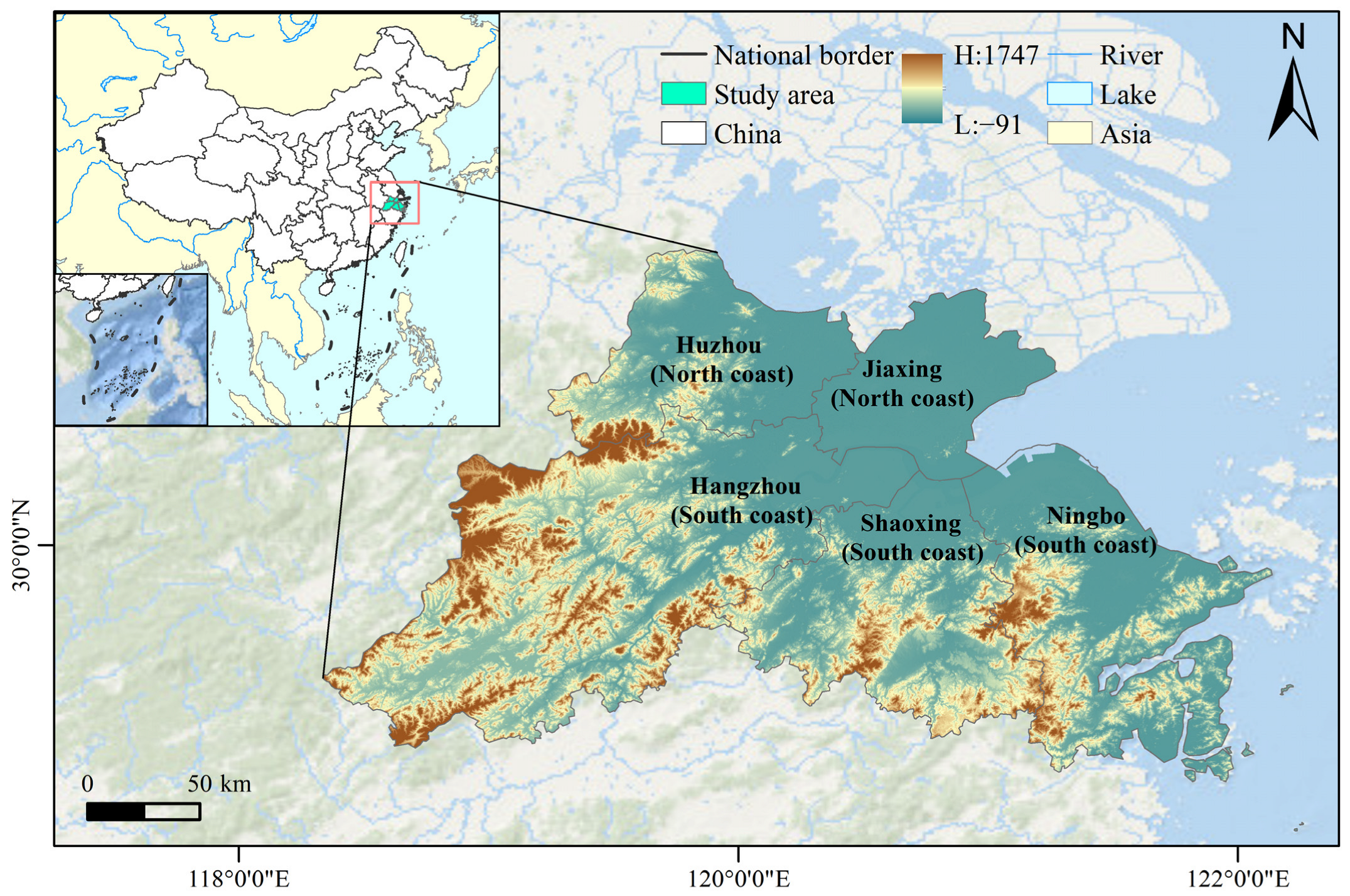
The region around Hangzhou Bay (29°51′–31°2′ N, 118°20′–123°25′ E) spans the five cities of Hangzhou, Ningbo, Jiaxing, Shaoxing, and Huzhou (Figure 1), with a total area of approximately 45,000 km², and constitutes an important component of the Yangtze River Delta Economic Zone.

The study area is restricted to the coastal land area of Hangzhou Bay, excluding the eastern island regions. Based on the morphological characteristics of Hangzhou Bay, the study area was divided into northern and southern coastal regions using the main trough of the bay as the boundary. Hangzhou Bay is a typical funnel-shaped bay [18], and its main channel serves as a conduit for tidal exchange and sediment transport [19]. Under long-term hydrodynamic forces, this channel has shaped a coastal landform pattern with marked differences between the northern and southern coasts, resulting in distinct variations in shoreline development, sedimentary environments, and land–sea interactions on both sides [20]. The northern coast is dominated by the Yangtze River Delta alluvial plain and features relatively flat topography, whereas the southern coast comprises both coastal plains and low mountains and hills. This results in a more undulating terrain that significantly influences land-use patterns and the evolution of the surface thermal environment. The northern coast includes Jiaxing and Huzhou, whereas the southern coast comprises Hangzhou, Shaoxing, and Ningbo; the corresponding zoning boundaries are shown in Figure 1.

The regional climate is characterized by a subtropical monsoon climate, with four distinct seasons and an average annual temperature of approximately 16 °C. The seabed topography in the eastern section of the bay mouth exhibits an alternating distribution of shallow beaches, sand ridges, and tidal gullies, with abundant tidal flat resources. From 1959 to 2019, tidal flats along the southern coast of Hangzhou Bay exhibited a trend of siltation and outward expansion, with the siltation rate accelerating to approximately 12.59 cm/y after 2003 [21].

2.2. Data Sources

The dataset used in this study comprises 12 categories, including LST, land use, population density (Pop), gross domestic product (GDP), vegetation cover, topography, and climate variables, as detailed in

Table 1. Data source.

Data Type	Data Product	Data Source	Spatial Resolution	Time
land surface temperature (LST)	MOD11A2	https://lpdaac.usgs.gov (accessed on 16 May 2025)	1 km	Summer (June–August) 2000–2020
Land use data	GLC_FCS30D	http://data.casearth.cn (accessed on 16 May 2025)	30 m	2000, 2005, 2010, 2015, and 2020
Population density (Pop)	LandScan Global Population Database	https://landscan.ornl.gov (accessed on 19 December 2025)	1 km	Same as above
Gross domestic product data (GDP)	National GDP raster data	National Tibetan Plateau Data Center (TPDC, https://data.tpdc.ac.cn (accessed on 19 December 2025)), Institute of Geographic Sciences and Natural Resources Research (IGSNRR), Chinese Academy of Sciences (CAS)	1 km	Same as above
Nighttime light data (NTL)	DMSP/OLS and NPP/VIIRS DNB nighttime light data	https://www.ngdc.noaa.gov/eog/ (accessed on 19 December 2025) https://eogdata.mines.edu/products/vnl/ (accessed on 19 December 2025)	1 km 500 m	Same as above
Impervious surface data (Normalized Difference Built-up Index, NDBI)	MOD09A1	https://search.earthdata.nasa.gov (accessed on 19 December 2025)	500 m	2000–2020
Albedo (AL)	MCD43A3	https://lpdaac.usgs.gov/ (accessed on 20 December 2025)	500m	Summer 2000–2020
Vegetation cover data (Normalized Difference Vegetation Index, NDVI)	MOD13A2	https://lpdaac.usgs.gov (accessed on 19 December 2025)	1 km	Same as above
Wind speed(WS)	ERA5 reanalysis data	https://cds.climate.copernicus.eu/ (accessed on 21 December 2025)	About 0.25°	Same as above
Relative humidity (RH)	ERA5 reanalysis data	https://cds.climate.copernicus.eu/ (accessed on 21 December 2025)	About 0.25°	Same as above
Elevation (EL)	SRTMGL1_003	https://search.earthdata.nasa.gov/ (accessed on 19 December 2025)	30 m	Static data
Slope (SLP)	DEM_HGT/001	https://search.earthdata.nasa.gov/ (accessed on 19 December 2025)	30 m	Same as above

.

2.3. Research Methods

2.3.1. Workflow

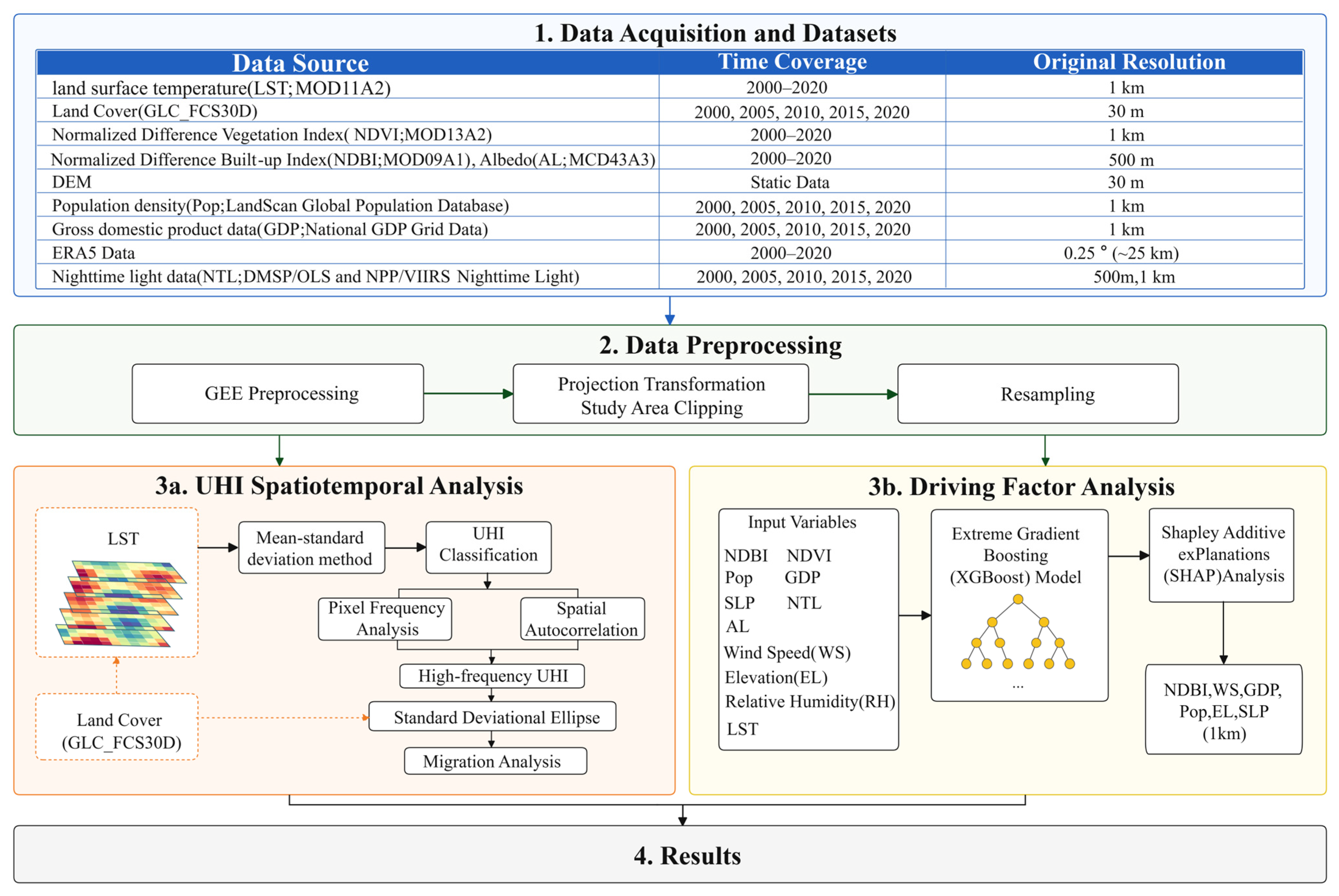
To investigate the spatiotemporal evolution and driving factors of the UHI effect in the urban agglomeration around Hangzhou Bay, this study developed the research framework shown in Figure 2. Based on MODIS LST data and multisource socioeconomic and natural environmental data, all datasets were first subjected to uniform preprocessing and spatial standardization. Subsequently, the mean-standard deviation method was used to classify heat islands, and their spatiotemporal patterns and migration characteristics were characterized using frequency statistics, spatial autocorrelation analysis, and the standard deviation ellipse method. Furthermore, the XGBoost-SHAP model was introduced to quantitatively analyze the contributions of multiple driving factors to surface temperature and to reveal their underlying mechanisms.

2.3.2. Data Preprocessing

1.

LST Data Preprocessing

This study utilized the Google Earth Engine (GEE) platform to obtain MOD11A2 LST products, uniformly selecting the daytime LST band (LST_Day_1km). All valid imagery acquired during the summer months (June–August) of each study year from 2000 to 2020 was extracted. After correction using a scaling factor, the data was converted to true surface temperature (°C) using Formula (1), and the average summer surface temperature was calculated on a pixel-by-pixel basis [22].

$$T_s=\mathit{DN} \times 0.02 - 273.15$$

(1)

where $T_s$ represents the true LST (unit: °C), and $\mathit{DN}$ represents the pixel gray value.

The MOD11A2 product employs cloud detection and quality-control algorithms and reduces the effects of cloud cover and short-term weather variations through 8-day compositing. This study did not perform additional spatial interpolation for missing pixels. Instead, the summer average LST was calculated directly using valid observations to avoid the additional uncertainty introduced by interpolation. Seasonal-scale averaging helps reduce random errors and improves the stability of regional thermal environment analysis.

2.

Auxiliary Data Processing

Using the MOD09A1 surface reflectance product, after removing the effects of clouds and cloud shadows using the StateQA bands, the Normalized Difference Building Index (NDBI) is calculated based on the shortwave infrared band (sur_refl_b06) and the near-infrared band (sur_refl_b02), using the following Formula (2) [23]:

$$\mathit{NDBI} = {\displaystyle \frac{\mathit{SWIR}-\mathit{NIR}}{\mathit{SWIR} + \mathit{NIR}}}$$

(2)

where, $\mathit{SWIR}$ represents short-wave infrared reflectance, and $\mathit{NIR}$ represents near-infrared reflectance.

The annual NDBI was calculated by taking the median of the annual NDBI images, as shown in Formula (3):

$${\mathit{NDBI}}_y = \mathrm{Median}({\mathit{NDBI}}_1, {\mathit{NDBI}}_2, \dots , {\mathit{NDBI}}_n)$$

(3)

where, ${\mathit{NDBI}}_y$ is the long-term median NDBI, ${\mathit{NDBI}}_i$ is the annual median NDBI for year $i$, $n$ is the total number of years.

The Normalized Difference Vegetation Index (NDVI) was derived from the MOD13A2 vegetation index product [24]. Summer (June–August) imagery for each year was extracted and corrected using a scaling factor shown in Formula (4):

$$\mathit{NDVI} = \mathit{DN} \times 0.0001$$

(4)

where, $\mathit{DN}$ represents the raw numerical value.

Summer NDVI is calculated using a mean-based composite, as shown in Formula (5):

$${\mathit{NDVI}}_{\mathit{JJA}} = {\displaystyle \frac{1}{n}}{\sum }_{i=1}^n{\mathit{NDVI}}_i$$

(5)

where, ${\mathit{NDVI}}_i$ represents the NDVI value of the $i$-th image, and $n$ represents the total number of valid summer images.

Wind speed (WS) and relative humidity (RH) were calculated using ERA5 Daily reanalysis data. WS was calculated according to Formula (6) [25]:

$$\mathit{WS} = \sqrt{u^2 + v^2}$$

(6)

where, $u$ and $v$ are the east–west and north–south WS components, respectively, at a height of 10 m.

RH was calculated using the Magnus Formula [26] (Formula (7):

$$\mathit{RH} = 100 \times {\displaystyle \frac{\exp \left(\frac{17.625T_d}{T_d + 243.04}\right)}{\exp \left(\frac{17.625T}{T + 243.04}\right)}}$$

(7)

where, $T$ and $T_d$ represent the 2 m air temperature and the 2 m dew point temperature (°C), respectively.

Daily data for the summer months (June–August) of each year were extracted, and seasonal averages were then calculated using Formula (8):

$$X_{\mathit{JJA}} = {\displaystyle \frac{1}{n}}{\sum }_{i=1}^n{X}_i$$

(8)

where, $X_{\mathit{JJA}}$ represents the seasonal average, $X_i$ represents the value of the variable on day $i$, and $n$ represents the total number of days in the daily summer dataset.

Nighttime light (NTL) data included DMSP-OLS (2000–2011) and NPP-VIIRS (2012–2020). The “stable lights” and “average radiance” bands were extracted from these datasets, respectively, and annual averages were calculated. The resulting annual nighttime light data were used to characterize the intensity of human activity in the region, as calculated using Formula (9):

$${\mathit{NTL}}_y = {\displaystyle \frac{1}{n}}{\sum }_{i=1}^n{\mathit{NTL}}_i$$

(9)

where, ${\mathit{NTL}}_y$ represents the NTL intensity in year $y$, ${\mathit{rNTL}}_i$ epresents the NTL image for the $i$-th period of that year, and $n$ represents the number of images for that year.

Surface albedo (AL) data were derived from the MCD43A3 albedo product [27]. Summer (June–August) imagery for each year was extracted and corrected using a scaling factor shown in Formula (10):

$$\mathit{AL} = \mathit{DN} \times 0.0001$$

(10)

Summer AL is calculated using a mean-based composite, as shown in Formula (11):

$${\mathit{Al}}_{\mathit{JJA} }= {\displaystyle \frac{1}{n}}{\displaystyle \sum _{i=1}^n}{\mathit{Al}}_i$$

(11)

where, ${\mathit{Al}}_i$ represents the AL value of the $i$-th image, and $n$ represents the total number of valid summer images.

Data on Pop, GDP, and NTL were selected from the years 2000, 2005, 2010, 2015, and 2020, respectively. A long-term socioeconomic activity intensity index was constructed by overlaying grids from multiple time periods to characterize the spatial accumulation of human activities during the study period. Using the MODIS surface temperature product (1 km) as the spatial reference, all driver data were resampled to a spatial resolution of 1 km. Continuous variables such as WS, RH, AL, elevation (EL), and slope (SLP) were resampled using bilinear interpolation, whereas NTL data were resampled using the nearest-neighbor interpolation method. This ensured spatial continuity for subsequent thermal environment analysis and the construction of the XGBoost-SHAP model. Land use data were obtained from the GLC_FCS30D product, and impervious surface data for the corresponding years were selected for spatial transfer analysis.

In addition to existing data products, the remaining data were primarily obtained and preprocessed using the GEE platform. All data were uniformly projected to the WGS1984 coordinate system to ensure spatial consistency and were cropped to the study area in ArcGIS 10.8.1.

2.3.3. Heat Island Intensity Classification Methodology

Based on the mean-standard deviation method [28], surface temperatures around the Hangzhou Bay region were classified into five heat island intensity levels (

Table 2. Heat island intensity classification.

Heat Island Level	Temperature Range
Strong cold island area	T < μ − 1.5 std
Cold island area	μ − 1.5 std ≤ T < μ − 0.5 std
Normal temperature zone	μ − 0.5 std ≤ T < μ + 0.5 std
Heat island area	μ + 0.5 std ≤ T < μ + 1.5 std
Strong heat island area	T ≥ μ + 1.5 std

Note: μ is the mean value; std is the standard deviation.

). Specifically, μ and std were calculated separately for each year across the entire study area using average summer (June–August) surface temperature images. The classification thresholds varied dynamically by year to eliminate the influence of interannual differences in absolute temperature values on the classification results.

To analyze interdecadal trends in the heat island effect, the frequency of occurrence of each heat island level was calculated on a pixel-by-pixel basis using annual classification results. The study period was divided into two phases, 2000–2010 and 2010–2020, and the frequency of heat island occurrence was calculated for each phase. Specifically, the heat island distribution results for all years within each phase were overlaid on a pixel-by-pixel basis, and the cumulative frequency of different heat island levels for each pixel was calculated to characterize the persistence of the heat island phenomenon.

To ensure comparability between the results across the two periods, a unified heat island frequency classification standard was adopted, dividing occurrences into levels 1–10, where Level 1 indicated the lowest frequency and Level 10 the highest. Higher levels indicated a more stable and persistent heat island phenomenon. Levels 1–3 represented low frequency, indicating sporadic occurrences; levels 4–7 represented medium frequency, indicating a certain degree of persistence but with fluctuations; and levels 8–10 represented high frequency, indicating persistent or recurrent occurrences with long-term stability. Based on this, a heat island frequency statistical map was generated (Formula (12)):

$$F_i = {\sum }_{t=1}^n{\mathrm{C}}_{i,t}$$

(12)

where, $F_i$ represents the frequency with which a pixel is classified into a specific heat island level during the study period. ${\mathrm{C}}_{i,t}$ is the classification value of pixel $i$ in year $t$ (if the pixel attribute belongs to the heat island category, the frequency increases by 1 time). $n$ represents the total number of years. The resulting frequency range (1–10) reflects the temporal stability of heat island distribution.

2.3.4. Spatial Autocorrelation Analysis and Standard Deviation Ellipse Analysis

Spatial autocorrelation analysis was employed to quantitatively characterize the spatial distribution of the surface thermal environment at both global and local scales, thereby revealing spatial clustering patterns of surface temperature within the study area [29,30]. The relevant calculation formulas are presented in Formulas (13) and (14).

$${\mathit{Moran}}^{\prime }I={\displaystyle \frac{n{\displaystyle {\sum }_{i=1}^n}{\sum }_{j=1}^n(x - \stackrel{\mathrm{-}}{x}\left)\right(x_j - \stackrel{\mathrm{-}}{x})}{({\displaystyle {\sum }_{i=1}^n}{\sum }_{j=1}^n{W}_{\mathit{ij}}){\sum }_{j=1}^n{\left(x_i - \stackrel{\mathrm{-}}{x}\right)}^2}}$$

(13)

$$I_i={\displaystyle \frac{(x_i-\stackrel{\mathrm{-}}{x})}{{\displaystyle {\sum }_j^n}{(x_j-\stackrel{\mathrm{-}}{x})}^2/n}}{\displaystyle \sum _{j=1,j\ne i}^n}{W}_{\mathit{ij}}(x_j-\stackrel{\mathrm{-}}{x})$$

(14)

where, $n$ represents the number of spatial elements, $x_i$ and $x_j$ are the attribute values of spatial elements $i$ and $j$, respectively, $\stackrel{\mathrm{-}}{x}$ is the mean of the attribute values across all spatial cells, and $W_{\mathit{ij}}$ is the spatial weight between spatial units $i$ and $j$, respectively. In the local spatial autocorrelation formula, $I_i$ represents the local autocorrelation index, $x_i$ and $x_j$ denote the attribute values of spatial units $i$ and $j$, and $\stackrel{\mathrm{-}}{x}$ indicates the average value. $n$ represents the total number of spatial units; $W_{\mathit{ij}}$ indicates the adjacency weight. When $I$ and $j$ are connected, $W_{\mathit{ij}}$ = 1; otherwise, $W_{\mathit{ij}}$ = 0 ($i$ = 1, 2, …), $n$, $j$ = 1, 2, … $m$), where $m$ is the number of adjacents.

On this basis, the standard deviation ellipse method was applied to describe the spatial distribution of strong heat islands and impervious surfaces across different periods [31,32]. The corresponding calculations are given in Formulas (15) and (16). Combined with center-of-gravity migration analysis, this approach was used to examine temporal evolution processes and to characterize the spatial relationship and evolutionary trends between the thermal environment and urban expansion.

$$\stackrel{\mathrm{-}}{\mathrm{X}}=\sqrt{{\displaystyle \frac{{\sum }_i^n{\left(x_i-x_j\right)}^2}{n}}}\stackrel{\mathrm{-}}{Y}=\sqrt{{\displaystyle \frac{{\sum }_i^n{\left(y_i-y_j\right)}^2}{n}}}$$

(15)

$$\left\{\begin{array}{c}\mathit{tan}\mathsf{\theta }={\displaystyle \frac{A+B}{\mathrm{C}}}, A=\left({\sum }_{i=1}^n{\tilde{x}}_t^2-{\sum }_{i=1}^n{{\tilde{y}}_t}^2\right)\\ B=\sqrt{{(\left({\sum }_{i=1}^n{\tilde{x}}_t^2-{\sum }_{i=1}^n{{\tilde{y}}_t}^2\right)}^2+4{\left({\sum }_{i=1}^n\widetilde{x_t}\widetilde{y_t}\right)}^2}\\ \mathrm{C}=2{\sum }_{i=1}^n\widetilde{x_t}\widetilde{y_t}\end{array}\right.$$

(16)

where, $x_i$ and $y_i$ are the coordinates of the $i$-th spatial cell, $\stackrel{\mathrm{-}}{\mathrm{X}}$ and $\stackrel{\mathrm{-}}{Y}$ are the geometric centers of the spatial distribution, $n$ is the total number of features, $\widetilde{x_t}$ and $\widetilde{y_t}$, are the coordinate offsets of the $i$-th feature relative to the center of mass, $\mathsf{\theta }$ is the rotation angle of the standard deviation ellipse; $A, B$ and $C$ are intermediate calculation variables used to determine the orientation angles of the ellipse.

2.3.5. Analysis of Driving Factors of the Heat Island Effect Based on the XGBoost-SHAP Model

To characterize the combined influence and nonlinear relationships among multiple environmental driving factors on LST during the formation of strong heat islands, an XGBoost regression model was constructed. XGBoost is an ensemble learning method based on boosting trees that can capture multifactor interactions, nonlinear relationships, and threshold effects without linear relationships among variables [33]. It is therefore well suited for modeling complex surface processes and environmental drivers. Its model formulation is as follows:

$$\widehat{Y} = {\sum }_{m=1}^M{f}_m\left(X\right)$$

(17)

where $\widehat{Y}$ denotes the LST forecast, $X$ denotes the input feature vector, $M$ denotes the total number of decision trees; $f_m$ denotes the $m$th CART regression tree model.

Although XGBoost effectively captures complex relationships between environmental factors and LST, its internal decision-making process lacks interpretability. To quantify the magnitude and direction of the influence of each environmental factor on LST, the SHAP method [34] was applied to interpret the XGBoost model outputs. SHAP is based on Shapley value theory from cooperative game theory and treats the predicted LST as the combined effect of multiple environmental factors. By computing the marginal contribution of each factor across different feature combinations, SHAP quantifies its average contribution to LST. This framework enables direct comparison of the relative importance of environmental drivers and reveals their nonlinear effects. The Shapley value is calculated as follows:

$${\mathsf{\varnothing }}_{\left(i\right)} = \sum _{S\subseteq N\left\{i\right\}}{\displaystyle \frac{\left|S\right|!\left(\left|N\right|-\left|S\right|-1\right)!}{\left|N\right|!}}\left(v\left(S\cup \left\{i\right\}-v\left(S\right)\right)\right)$$

(18)

where ${\mathsf{\varnothing }}_{\left(i\right)}$ is the contribution value of the $i$-th feature, $N$ represents the set of all features; $S$ is any feature subset that does not contain feature $i$, and $\left|S\right|$ is the number of features in the set $S$. $v\left(S\right)$ represents the contribution of set $S$ to the model prediction output; $\left|N\right|$ is the total number of features; and $\left(v\left(S\cup \left\{i\right\}-v\left(S\right)\right)\right)$ represents the marginal contribution.

2.3.6. Model Implementation

In this study, LST was used as the dependent variable, and 10 environmental factors were selected as independent variables. Valid pixel samples were extracted from multi-source raster data to serve as the model’s input dataset. After data preprocessing, a total of 25,781 valid samples were obtained and randomly divided into training and testing sets in an 8:2 ratio for model training and validation.

Based on this, a filtering feature selection method using Spearman’s rank correlation coefficient was employed to preliminarily screen the variables, thereby reducing the impact of multicollinearity and enhancing model stability. The screened variables were then input into an XGBoost model constructed with XGBRegressor. The number of estimators was set to 100, the maximum decision tree depth to 3, and the learning rate to 0.1. During model training, hyperparameters were tuned using Random Search combined with 5-fold cross-validation. A total of 30 parameter combinations were tested, and negative mean squared error (neg_mean_squared_error) was selected as the optimization objective function. The specific parameter settings are shown in

Table 3. Parameter setting of the model.

Hyperparameter	Description	Search Space
nrounds	Number of estimators	50–200
max_depth	Maximum depth of the tree	4–8
min_child_weight	Minimum number of samples on leaf nodes	1–5
gamma	Minimum loss reduction for split nodes	0–0.2
colsample_bytree	Proportion of random sample columns used per tree	0.7–1
subsample	Proportion of random sample observations per tree	0.7–1
alpha	The weight coefficient of the L1 regularization term	0.5
lambda	The weight coefficient of the L2 regularization term	0.5–2.0

. The model’s accuracy was evaluated using the coefficient of determination (R²), root mean square error (RMSE), and mean absolute error (MAE). To further interpret the model’s predictions, the SHAP algorithm was used to assess the importance of these factors. All modeling, training, prediction, and interpretability analyses were conducted in Python 3.10. Shapley values were computed using the KernelExplainer class from the SHAP package.

3. Results and Analysis

3.1. Spatiotemporal Variation Analysis of Heat Island Intensity Around Hangzhou Bay

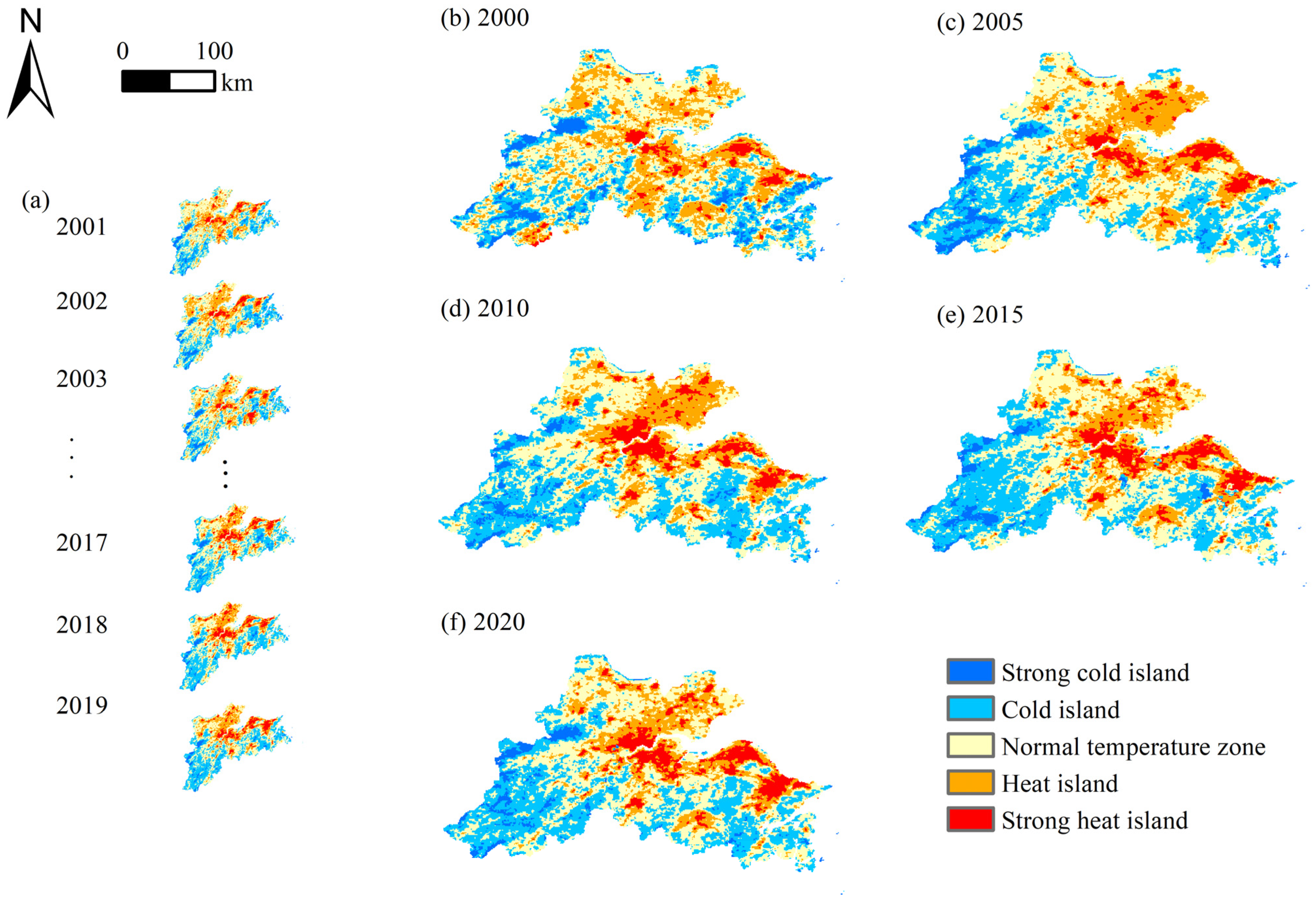
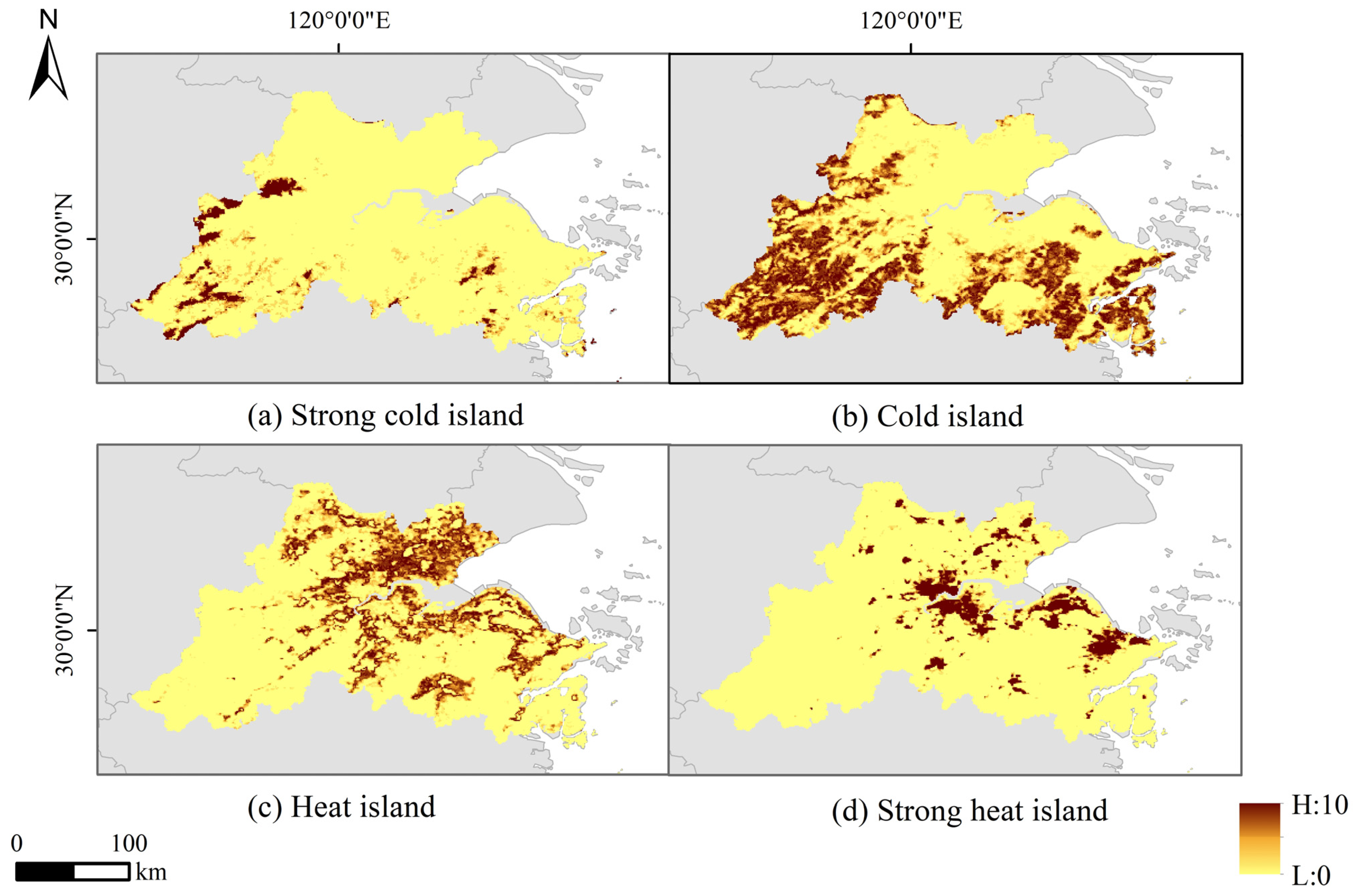
From 2000 to 2020, the high-frequency areas of both heat islands and strong heat islands in the region around Hangzhou Bay expanded markedly. With increasing thermal intensity, portions of heat island areas progressively transitioned into strong heat islands. In terms of spatial evolution, strong heat islands were initially concentrated within core built-up areas in a point-like pattern, subsequently expanding into coastal industrial zones and gradually coalescing into contiguous, surface-like distributions. Concurrently, heat island areas expanded outward from strong heat island cores and extended along urban development axes, forming a continuous expansion pattern (Figure 3).

Over the same period, areas corresponding to different heat island grades exhibited distinct stage-wise dynamics. From 2000 to 2010, the area classified as heat island decreased by 2086 km², whereas the strong heat island area increased substantially by 1889 km². During this interval, the cold island area increased by 4261 km², while the strong cold island area decreased by 1308 km². From 2010 to 2020, the heat island area increased marginally by 55 km², and the strong heat island area continued to expand by 516 km², whereas the cold island and strong cold island areas decreased by 185 km² and 60 km², respectively. Overall, high-temperature regions continued to expand, although the rate of change declined.

Temporal Expansion Characteristics of Different Heat Island Level Frequencies

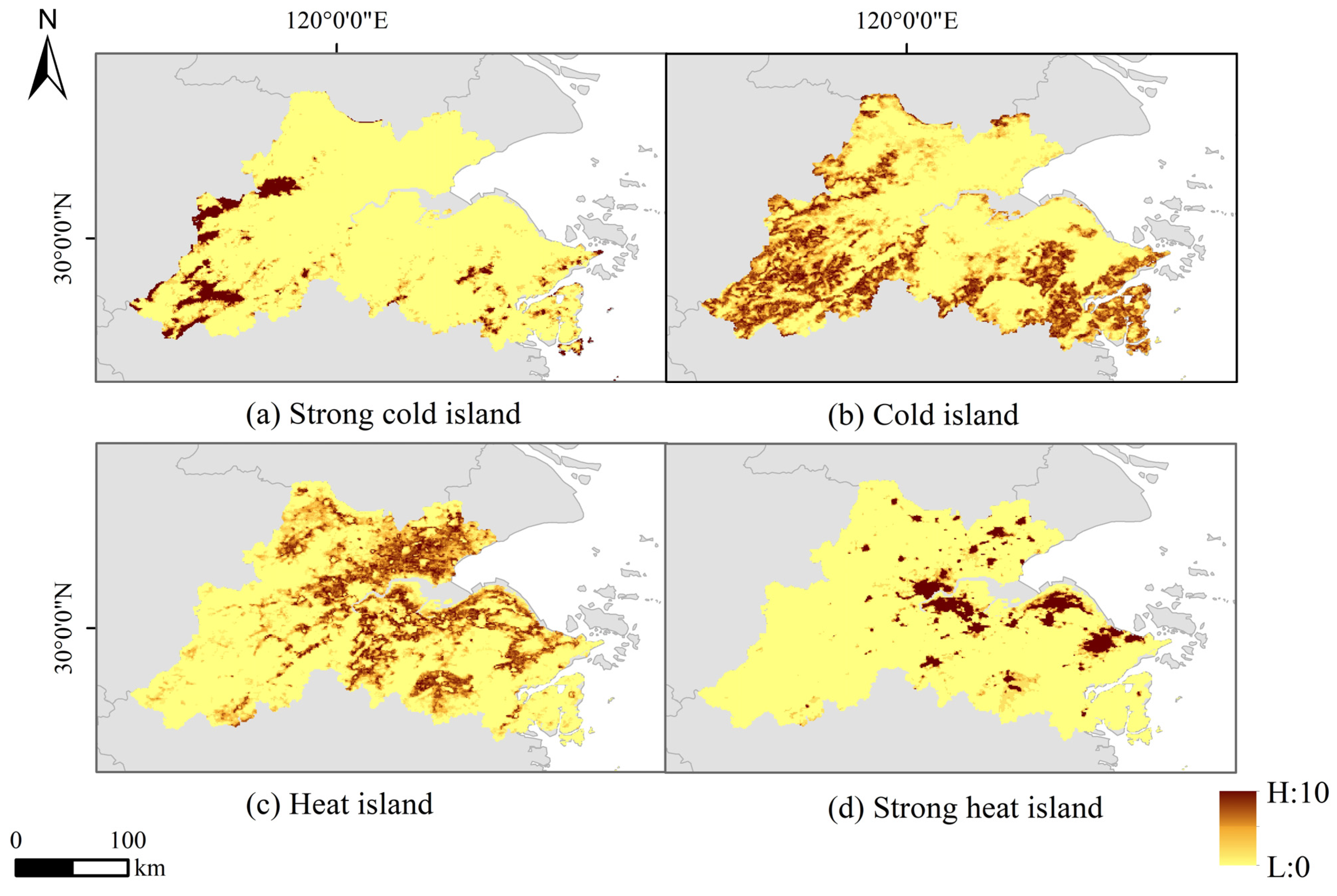
Based on pixel-level frequency statistics from 2000 to 2020 (Figure 4 and Figure 5), high-frequency occurrence areas of both heat island and strong heat island classes exhibited sustained expansion. The high-frequency heat island area increased from 4779 km² to 6328 km² (32.41%), while the high-frequency strong heat island area expanded from 2042 km² to 3310 km² (62.10%). Compared with the heat island class, the strong heat island class demonstrated more pronounced long-term spatial expansion. Spatially, high-frequency high-temperature zones remained concentrated in core cities, including Hangzhou and Ningbo, while progressively forming continuous belts along the peripheries of built-up areas.

In contrast, cold island and strong cold island classes generally exhibited contraction. During the study period, the low-frequency cold island area decreased by 2812 km² (26.81%), and the medium-frequency area decreased by 2380 km² (23.61%), whereas the high-frequency cold island area increased by 70.37%. This pattern indicates an overall contraction in cold island extent, accompanied by the persistence and localized intensification of core areas. Conversely, the high-frequency strong cold island area decreased significantly by 38.27%, with a marked reduction in spatial continuity and aggregation. Spatially, cold islands and strong cold islands were primarily distributed in ecologically favorable western and southern regions; however, strong cold islands exhibited greater shrinkage and fragmentation.

3.2. Spatial Aggregation Characteristics of Heat Island Distribution Around Hangzhou Bay

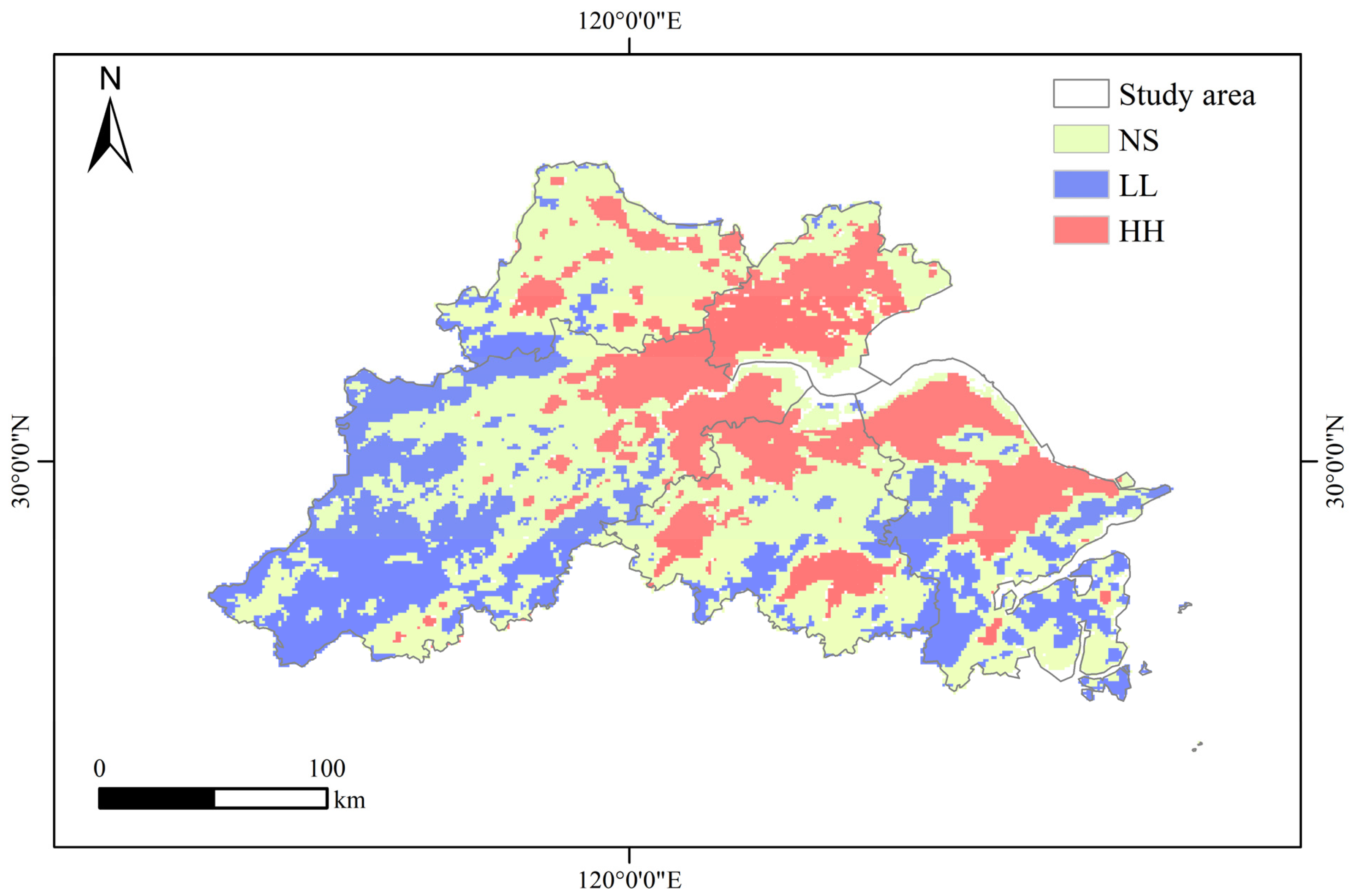
The global spatial autocorrelation statistic, Moran’s I, of LST in the region around Hangzhou Bay region was 0.93 (p < 0.01), indicating strong positive spatial autocorrelation and significant clustering of heat island patterns. Local spatial autocorrelation (LISA) analysis identified two dominant clustering types: high–high clusters, where high-temperature pixels are surrounded by similarly high-temperature pixels, representing persistent heat island cores; and low–low clusters, where low-temperature pixels are surrounded by low-temperature pixels, corresponding to stable cold island areas.

Heat island regions exhibited a typical high–high clustering pattern, characterized by a multi-centered structure aligned along urban development axes. These clusters were primarily located in built-up areas such as northeastern Hangzhou, northern Ningbo, and southern Jiaxing, including Hangzhou Qiantang New Area, Ningbo Hangzhou Bay New Area, and Jiaxing Binhai New Area (Figure 6). These areas are characterized by high building density and population concentration, resulting in elevated surface temperatures and pronounced clustering. In contrast, cold island regions exhibited low–low clustering patterns, mainly distributed in forested and water-rich areas, including the western mountainous regions of Hangzhou (e.g., Tianmu Mountains), the southern hills and wetlands of Ningbo (e.g., Dongqianhu Lake and Siming Mountain), and the northern wetland regions of Jiaxing (e.g., Jiashan wetland clusters). These areas are characterized by high vegetation cover, complex terrain, and lower surface temperatures, forming stable low–low clustering patterns.

3.3. Spatial Distribution Variation Trend of Strong Heat Islands and Impervious Surfaces

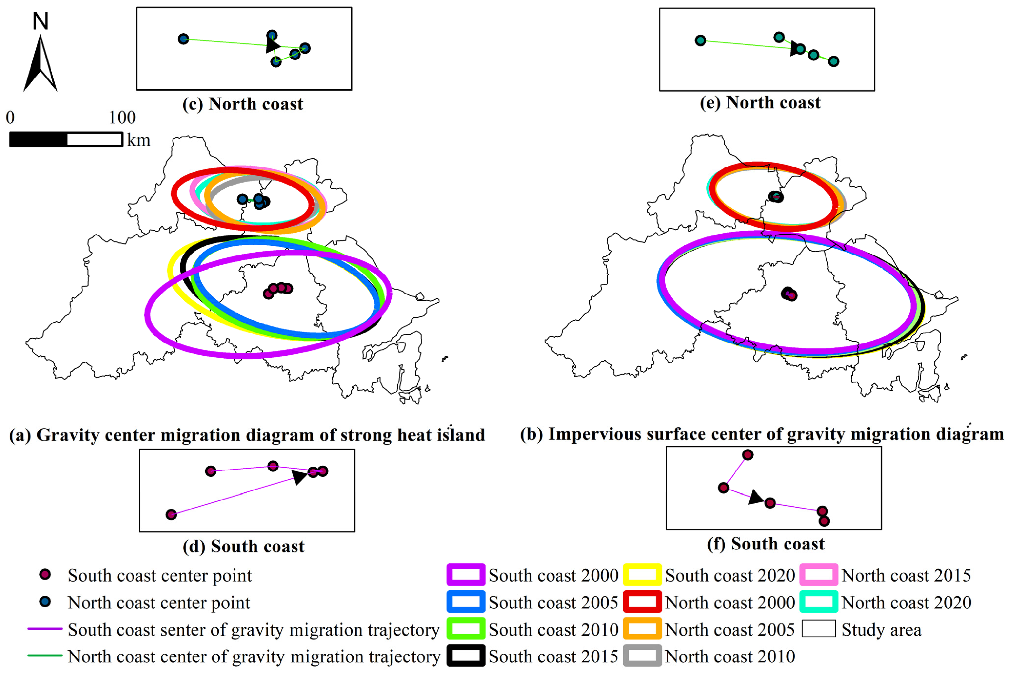
From 2000 to 2020, the migration of the centers of gravity of strong heat islands and impervious surfaces exhibited an overall positive spatial correlation in the Hangzhou Bay region, although notable regional differences were observed (Figure 7;

Table 4. Migration rate of the center of gravity of the impervious surface and strong heat island on the north and south coasts in different periods.

Time Interval	North Coast Impervious Surface	North Coast Strong Heat Island	South Coast Impervious Surface	South Coast Strong Heat Island
2000–2005	3.05	19.90	1.66	21.27
2005–2010	1.08	2.05	2.29	1.06
2010–2015	0.63	3.40	2.48	5.55
2015–2020	1.19	5.07	0.47	7.00
2000–2005	3.05	19.9	1.66	21.27

).

On the northern coast, both strong heat islands and impervious surfaces exhibited consistent southeastward migration toward Hangzhou Bay. The center of gravity of strong heat islands shifted by 30.42 km, whereas that of impervious surfaces moved by 5.95 km. On the southern coast, both exhibited similar southeastward migration from 2000 to 2010, with shifts of 22.33 km (strong heat islands) and 3.95 km (impervious surfaces). However, after 2010, the migration direction of strong heat islands reversed, diverging from the continued southeastward movement of impervious surfaces. During this phase, the strong heat island center shifted by 12.55 km, while the impervious surface center shifted by 2.95 km.

In terms of migration rates, strong heat islands consistently exhibited higher movement rates than impervious surfaces; however, this difference diminished after 2005. From 2000 to 2005, the migration rate of strong heat islands on the northern coast was approximately 6.53-fold higher than that of impervious surfaces, and 12.81-fold higher on the southern coast. From 2010 to 2020, the migration speed of the strong heat islands on the northern and southern coasts remained significantly higher than that of impervious surfaces, at 4.25- and 4.65-fold times on the northern and southern coasts, respectively. Notably, the southern coast exhibited more pronounced divergence in trends: the migration rate of strong heat islands increased from 1.11 km/5a to 1.38 km/5a between 2010 and 2020, whereas the impervious surface migration rate decreased from 0.50 km/5a to 0.09 km/5a.

The migration trajectory of strong heat islands on the southern coast exhibited clear phase-dependent behavior, initially moving northeastward before reversing toward the northwest. From 2000 to 2005, the center of gravity shifted rapidly northeastward along an extended trajectory. After 2010, the migration path shifted inland toward the northwest and southwest, deviating from the primary axis of coastal urban development.

3.4. Analysis of XGBoost-SHAP Model Results

After hyperparameter tuning, the final optimal parameters were as follows: subsample = 0.9, reg_lambda = 1.0, reg_alpha = 0.5, n_estimators = 150, min_child_weight = 1, max_depth = 8, gamma = 0.05, colsample_bytree = 1.0. The model achieved RMSE = 0.4774, MAE = 0.3586, and R² = 0.9470 on the training set, and RMSE = 0.7385, MAE = 0.5569, and R² = 0.8704 on the test set, indicating that the model has a high fitting ability and good generalization performance. The influence of the above-mentioned environmental factors mentioned above on LST can therefore be explained.

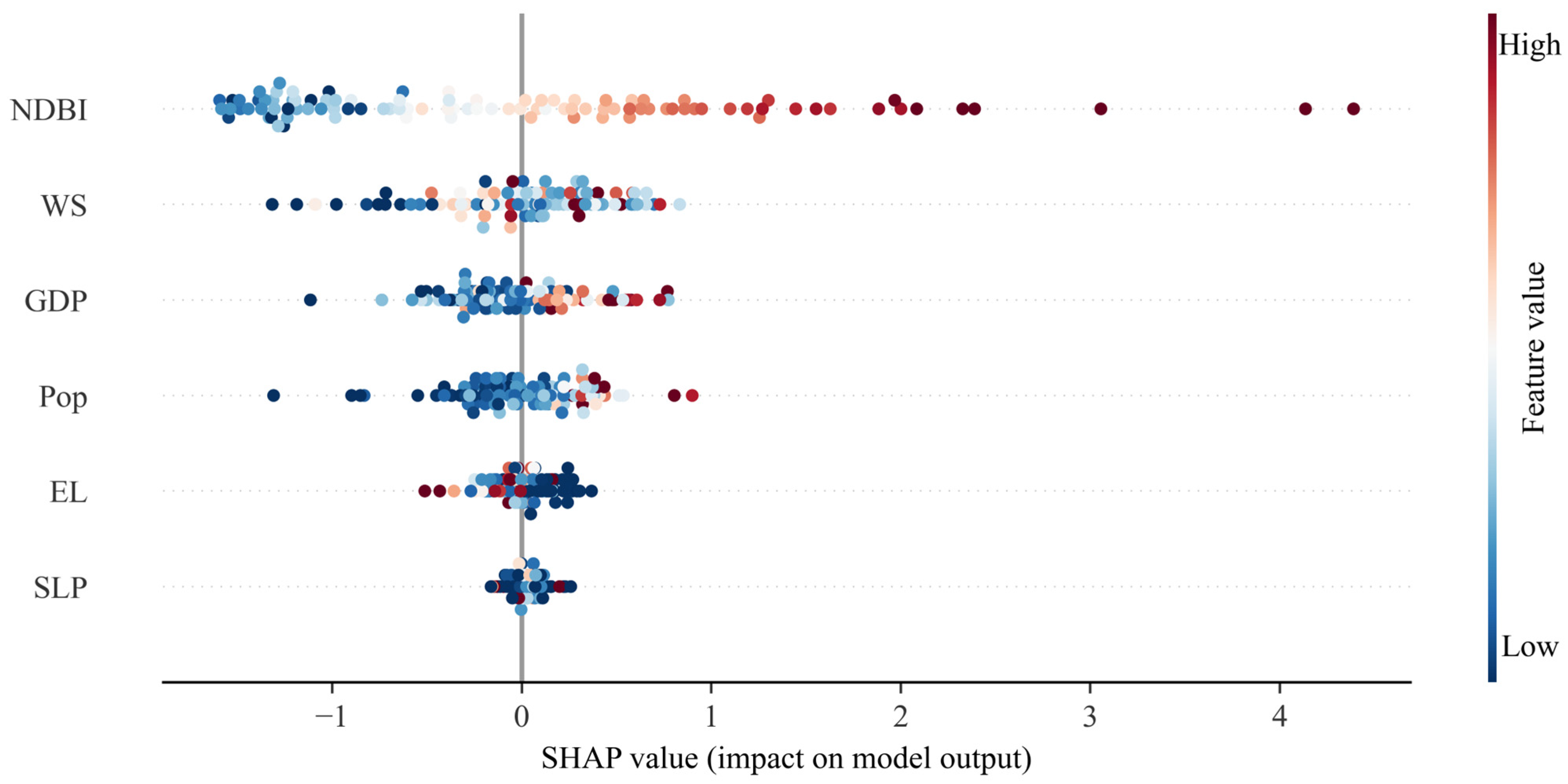
In terms of variable screening, six explanatory variables were ultimately retained, namely NDBI, WS, GDP, Pop, EL, and SLP. The SHAP analysis results showed significant differences in the contribution of each variable to surface temperature. Among them, NDBI had the highest contribution (0.8923), followed by WS (0.3612), GDP (0.2358), Pop (0.2276), EL (0.1109), and SLP (0.0623). Notably, although vegetation cover exerts a significant moderating effect on surface temperature, it was excluded during variable screening. This was primarily because the variable selection process employed a filtering method based on Spearman’s correlation coefficient. There was strong multicollinearity between the vegetation index and land surface characteristics such as NDBI; furthermore, its correlation with LST ranked relatively low among ecoclimatic variables, placing it outside the scope of priority selection for this category. Therefore, it was not included in the final optimal set of variables.

The analysis was conducted using the SHAP algorithm (Figure 8), which quantifies both the magnitude and direction of each variable’s contribution to LST predictions. Larger SHAP importance values indicate a greater influence on the spatial distribution of surface temperature, while the sign of SHAP values reflects warming (positive) or cooling (negative) effects, and their absolute magnitude represents contribution intensity. Further analysis of the SHAP results revealed that the explanatory variables differed not only in feature importance but also in their SHAP value distributions. NDBI had the highest SHAP feature importance, and its SHAP values exhibited a relatively wide distribution range. The SHAP values corresponding to high-value samples were mainly concentrated in the positive region, whereas those corresponding to low-value samples were more frequently distributed in the negative region, indicating a clear positive correlation between NDBI and the model prediction results. WS ranked second in importance. SHAP values differ significantly across different WS conditions. Specifically, samples with high WS were primarily distributed in the negative SHAP region, whereas samples with low WS were more frequently associated with positive SHAP values. GDP and Pop exhibited similar levels of importance and showed distribution patterns broadly comparable to those observed for NDBI. However, their SHAP value ranges were considerably narrower, and the corresponding SHAP values were distributed more continuously across the feature space. In contrast, the SHAP values of EL and SLP were mainly concentrated around zero, with relatively small fluctuation ranges and lower contributions to model predictions. Overall, the SHAP value distributions differed substantially among explanatory variables, reflecting varying association patterns between each variable and the model prediction results.

4. Discussion

4.1. Correlation Between Urbanization and Regional Thermal Environmental Change

With the advancement of urbanization, large areas of natural land have been converted into urban construction land. This transformation has altered the land use/land cover characteristics of the underlying surface, thereby affecting LST. According to the XGBoost-SHAP results, NDBI exhibited the highest feature importance. Increasing NDBI values were associated with significant increases in surface temperature, indicating that urban spatial expansion is the dominant driver of regional thermal environment intensification. This finding is consistent with those of Shen et al. [35,36]. During the study period, the built-up area around Hangzhou Bay increased by more than threefold. The rapid expansion of impervious surfaces substantially altered surface thermal capacity characteristics, intensified vegetation fragmentation [37,38], and enhanced continuous enhancement of surface heat accumulation.

High-frequency strong heat island areas are primarily concentrated in core cities such as Hangzhou and Ningbo, as well as in coastal industrial agglomeration belts, where the proportion of impervious surfaces within built-up areas has remained consistently high. The warming effect of newly developed construction land on the surface thermal environment intensified progressively during urbanization. In contrast, in regions with more favorable ecological conditions and more dispersed built-up areas, the influence of impervious surface expansion on surface temperature is comparatively limited. This indicates clear regional heterogeneity in thermal responses to urbanization. The strong spatial consistency between the migration trajectories of strong heat islands and impervious surfaces on the northern coast further confirms the dominant role of construction land expansion in driving strong heat island migration [39].

In addition to land-cover change, socioeconomic development also has a significant influence on the regional thermal environment. The SHAP analysis results indicated that both GDP and Pop exert positive effects, suggesting that economic growth and population concentration further intensify regional warming. This finding is consistent with that of Liu et al. [40]. During the study period, sustained economic growth in the Hangzhou Bay region promoted population concentration in urban areas and fueled the continuous expansion of construction activities and energy consumption. This further intensified intensifying the regional thermal environment. Unlike NDBI, which directly alters surface thermal characteristics, Pop and GDP primarily influence the regional thermal environment indirectly through increased anthropogenic heat emissions, intensified transportation activities, and rising energy consumption.

Adjustments in urban functional zoning further exacerbate thermal environmental pressures. During the early stage of the study period, the migration rates of the centers of gravity of strong heat islands on the northern and southern coasts were approximately 6.52 and 12.81 times higher than those of impervious surfaces, respectively. Although this disparity decreased in later stages, the migration rates of strong heat islands remained 4.65 and 4.25 times higher than those of impervious surfaces on the northern and southern coasts, respectively. These findings indicate that the formation and migration of strong heat islands are not solely governed by urban expansion and changes in the underlying surface. They are also influenced by dynamic adjustments in urban functional zoning, short-term agglomeration or redistribution of population and industry, and variations in energy consumption. Together, these factors further intensify urban thermal environmental conditions [41,42,43].

4.2. Local Cooling Effect on the Southern Coast Driven by Land–Sea Interactions

After 2010, the migration direction of the center of gravity of strong heat islands on the southern coast diverged from that of impervious surfaces, shifting from a seaward to a landward direction. Concurrently, migration rates also differed significantly from those of impervious surfaces. This indicates that, during the later stage of the study period, the migration of strong heat islands on the southern coast was no longer primarily driven by urban expansion. Instead, it was influenced by additional dominant factors.

This shift is closely associated with the distinct land–sea interaction processes operating within the study area. Extensive silted tidal flat wetlands have developed along the southern coast of Hangzhou Bay, with their area increasing by 409.19% between 1998 and 2013 [44]. These wetlands constitute an important regional cooling source. Tidal flat accretion, wetland expansion, and thermal contrasts between land and sea have significantly altered subsurface conditions and regional energy exchange processes. Consequently, they have influenced both the local thermal environment and the migration of strong heat island centers. On the one hand, large-scale wetland expansion modifies surface roughness and thermal boundary conditions, increases latent heat flux, and reduces sensible heat accumulation, thereby lowering surface temperatures. On the other hand, enhanced sea-breeze circulation improves coastal ventilation efficiency, facilitates heat dissipation toward the sea and weakens coastal heat island intensity.

Under these combined influences, the center of gravity of strong heat islands migrates seaward in response to increasing impervious surfaces during periods dominated by urban expansion. However, when wetland expansion and oceanic regulation intensify, the cooling effect becomes stronger. This reduces heat accumulation in coastal zones and drives a landward shift in the heat island center. Therefore, the increase in migration rate observed along the southern coast after 2010, despite reduced impervious surface expansion, reflects the combined influence of urbanization and the dynamic evolution of coastal geomorphology [21].

From a long-term perspective, continued tidal flat accretion or land reclamation is likely to maintain dynamic adjustments in subsurface conditions. This may result in a cyclical, “pendulum-like” migration of strong heat island centers, shifting seaward under urban expansion and returning landward under wetland expansion and enhanced oceanic regulation. From a land–sea interaction perspective, coastal tidal flat wetlands along the southern coast of Hangzhou Bay function not only as key ecological components but also as critical regulators of the thermal environment in coastal urban systems. This regulatory effect partially offsets the warming associated with impervious surface expansion during urbanization. As a result, the thermal environment on the southern coast follows an evolutionary pathway that differs from that of typical inland urban expansion patterns.

4.3. Implications for Future Urban Planning Around Hangzhou Bay

The study shows that strong heat island areas are highly clustered within urban cores. Furthermore, the NDBI, GDP, and Pop all exert positive effects on surface temperature, with NDBI contributing the most. This indicates that the expansion of built-up areas remains the dominant driver of the regional thermal environment warming, whereas the concentration of economic activity and population growth further amplify this warming effect. Therefore, future urban planning around Hangzhou Bay should strictly control the disorderly expansion of impervious surfaces in core urban cores by increasing land-use intensity and optimizing urban functions and spatial layouts. In addition, the high spatial consistency between cold island areas and ecological land-use types, such as woodlands and wetlands, highlights the fundamental role of ecological land in regulating the urban thermal environment. In the context of rapid coastal urbanization, ecological spaces should be incorporated into the thermal environment regulation strategies. The protection of woodlands, wetlands, and coastal ecosystems should be strengthened to prevent encroachment by construction land. The spatial connectivity and diffusion capacity of cold island effects should be enhanced through the development of a multilevel ecological network to mitigate heat accumulation in urban cores.

Furthermore, both GDP and Pop exert positive effects on surface temperature, indicating that the concentration of economic activity and population growth may further exacerbate thermal environmental risks in the Hangzhou Bay region. Therefore, heat island mitigation efforts should identify “high heat–high exposure” composite risk areas by considering population density and industrial distribution. Core cities such as Hangzhou and Ningbo, as well as coastal industrial belts, are not only areas of high heat island intensity but also major zones of continued population inflow and intensive production activities. In these areas, high-temperature conditions are more likely to translate into actual heat exposure risks. Accordingly, cooling-oriented interventions should be prioritized in urban planning, including improving access to public spaces, optimizing pedestrian and slow-traffic systems, and enhancing shading and ventilation conditions. These measures can reduce both the duration and intensity of human exposure to high-temperature environments. At the industrial planning level, the spatial distribution of energy-intensive industries should be optimized to reduce anthropogenic heat emissions in areas with high GDP.

WS is the second most important factor affecting surface temperature, indicating that coastal meteorological conditions play a significant role in regulating the regional thermal environment. The Hangzhou Bay region is strongly influenced by land–sea breeze circulation. Therefore, urban planning should emphasize the construction and protection of ventilation corridors and strictly control the continuous development of high-density building clusters along prevailing wind directions. Future planning should integrate the regulatory role of southern coastal mudflats with the development of continuous ecological buffer zones and corridors between construction land and coastal ecosystems. This would enhance the transport and regulatory capacity of land–sea breezes. Furthermore, maintaining the ventilation and cooling functions of coastal ecosystems requires the protection of mudflats, restoration of salt marsh vegetation, and improvement of estuarine wetland connectivity. Together, these measures contribute to mitigating the UHI effect.

The observed directional shift in strong heat islands on the southern coast indicates that mudflat siltation within the land–sea transition zone exerts a significant regulatory influence on the regional thermal environment. Future finding suggests that future development intensity along the southern coast and adjacent nearshore areas of Hangzhou Bay should be scientifically regulated to avoid excessive seaward expansion of built-up land, thereby preserving the regulatory function of the land–sea transition zone in limiting heat island expansion. At the same time, mudflats and adjacent areas should be incorporated into an integrated system of ecological security and thermal environment regulation. This will help maintain long-term, stable thermal buffer zones for coastal new towns and industrial areas by preserving the continuity and integrity of coastal spatial structures.

4.4. Limitations of the Study and Future Directions

This study reveals the spatiotemporal evolution characteristics and driving factors of the UHI effect in the urban agglomeration around Hangzhou Bay at the regional scale. It also identifies an association between the migration of strong heat islands along the southern coast and changes in coastal tidal flat wetlands. However, although this study focuses on the overall evolution patterns of the regional thermal environment, it does not provide a quantitative assessment of the specific contribution of coastal wetlands to thermal regulation. Future studies integrating high-resolution remote sensing data, wetland dynamics monitoring data, and marine meteorological data could further elucidate the mechanisms through which changes in coastal wetlands influence the regional thermal environment. Such efforts would provide a stronger scientific basis for ecological conservation and thermal environment optimization along the Hangzhou Bay coast.

5. Conclusions

Based on MODIS LST data from 2000 to 2020, this study integrates the mean-standard deviation method, pixel-level frequency statistics, standard deviation ellipse analysis, spatial autocorrelation analysis, and the XGBoost-SHAP model, to systematically investigate the spatiotemporal characteristics of heat islands and their driving mechanisms in the Hangzhou Bay urban agglomeration.

The results show that high-frequency strong heat island areas expanded significantly during the study period, extending from early built-up areas to newly developed coastal zones. Spatial patterns evolved from discrete point distributions to contiguous areal agglomerations. Differences were observed in both the direction and rate of center-of-gravity migration between strong heat islands and impervious surfaces. Specifically, the northern coast was primarily influenced by urban expansion, whereas the southern coast exhibited clear phase-dependent shifts, indicating that changes in coastal tidal flats and wetlands play an important regulatory role in the local thermal environment. Driving factor analysis indicates that impervious surfaces (represented by NDBI) are the dominant factor influencing surface temperature, while WS plays a significant role in moderating the local thermal environment.

The study findings indicate that, in the region around Hangzhou Bay, urban expansion and changes in the coastal ecological environment jointly influence the regional thermal environment pattern. These findings can serve as a scientific reference for thermal environment management, coastal ecological conservation, and land-use planning in the Hangzhou Bay region. Future development in the urban agglomeration around Hangzhou Bay should fully consider the influence of land–sea interactions on thermal environment evolution. While advancing urban construction and industrial development, efforts should strengthen the protection of tidal flat wetlands and coastal ecological spaces and promote coordination among ecological conservation, thermal environment regulation, and territorial spatial planning to enhance regional ecological security and sustainable development.

References

1. Joshi, K.; Khan, A.; Anand, P.; Sen, J. Understanding the synergy between heat waves and the built environment: A three-decade systematic review informing policies for mitigating urban heat island in cities. Sustain. Earth Rev. 2024, 7, 25. [Google Scholar] [CrossRef]
2. Perkins-Kirkpatrick, S.E.; Lewis, S.C. Increasing trends in regional heatwaves. Nat. Commun. 2020, 11, 3357. [Google Scholar] [CrossRef] [PubMed]
3. Zhou, Z.; Zhang, L.; Zhang, Q.; Hu, C.; Wang, G.; She, D.; Chen, J. Global increase in future compound heat stress-heavy precipitation hazards and associated socio-ecosystem risks. npj Clim. Atmos. Sci. 2024, 7, 33. [Google Scholar] [CrossRef]
4. Gupta, A.; De, B.; Das, S.; Mukherjee, M. Thermal hazards in urban spaces: A review of climate-resilient planning and design to reduce the heat stress. Urban Clim. 2025, 59, 102296. [Google Scholar] [CrossRef]
5. Imran, H.M.; Kala, J.; Ng, A.W.M.; Muthukumaran, S. Impacts of future urban expansion on urban heat island effects during heatwave events in the city of Melbourne in southeast Australia. Q. J. R. Meteorol. Soc. 2019, 145, 2586–2602. [Google Scholar] [CrossRef]
6. Vujovic, S.; Haddad, B.; Karaky, H.; Sebaibi, N.; Boutouil, M. Urban heat island: Causes, consequences, and mitigation measures with emphasis on reflective and permeable pavements. CivilEng 2021, 2, 459–484. [Google Scholar] [CrossRef]
7. Li, W.; Han, C.; Li, W.; Zhou, W.; Han, L. Multi-scale effects of urban agglomeration on thermal environment: A case of the Yangtze River Delta megaregion, China. Sci. Total Environ. 2020, 713, 136556. [Google Scholar] [CrossRef] [PubMed]
8. Morabito, M.; Crisci, A.; Guerri, G.; Messeri, A.; Congedo, L.; Munafò, M. Surface urban heat islands in Italian metropolitan cities: Tree cover and impervious surface influences. Sci. Total Environ. 2021, 751, 142334. [Google Scholar] [CrossRef] [PubMed]
9. Fang, W.; Cao, J.; Biswas, A.; Feng, Q.; Wang, Y. Impacts of coordinated development policies on urban heat islands in the Beijing-Tianjin-Hebei urban agglomeration, China. Sustain. Cities Soc. 2024, 112, 105614. [Google Scholar] [CrossRef]
10. Wong, N.H.; Tan, C.L.; Kolokotsa, D.D.; Takebayashi, H. Greenery as a mitigation and adaptation strategy to urban heat. Nat. Rev. Earth Environ. 2021, 2, 166–181. [Google Scholar] [CrossRef]
11. Qiu, Y.F.F.; He, B.J. Review of urban water thermal environment cooling. IOP Conf. Ser. Earth Environ. Sci. 2024, 1363, 012073. [Google Scholar] [CrossRef]
12. Santamouris, M.; Vasilakopoulou, K. Urban climate and heat mitigation in coastal cities. In The Blue Book: Smart Sustainable Coastal Cities and Blue Growth Strategies for Marine and Maritime Environments; Rassia, S.T., Ed.; Springer International Publishing: Cham, Switzerland, 2024; pp. 79–85. [Google Scholar]
13. Yu, J.; Zhao, Q.; Gao, L.; Meng, Q.; Lei, X. Surface urban heat islands in coastal and inland cities: A global analysis of drivers and of spatial heterogeneity. Build. Environ. 2026, 301, 114751. [Google Scholar] [CrossRef]
14. Yin, Z.; Liu, Z.; Liu, X.; Zheng, W.; Yin, L. Urban heat islands and their effects on thermal comfort in the US: New York and New Jersey. Ecol. Indic. 2023, 154, 110765. [Google Scholar] [CrossRef]
15. Kawamoto, Y. Effect of land-use change on the urban heat island in the Fukuoka–Kitakyushu metropolitan area, Japan. Sustainability 2017, 9, 1521. [Google Scholar] [CrossRef]
16. Lauwaet, D.; Berckmans, J.; Hooyberghs, H.; Wouters, H.; Driesen, G.; Lefebre, F.; De Ridder, K. High resolution modelling of the urban heat island of 100 European cities. Urban Clim. 2024, 54, 101850. [Google Scholar] [CrossRef]
17. Meng, F.; Qi, L.; Li, H.; Yang, X.; Liu, J. Spatiotemporal evolution and influencing factors of heat island intensity in the Yangtze River Delta urban agglomeration based on GEE. Atmosphere 2024, 15, 1080. [Google Scholar] [CrossRef]
18. Xie, D.; Wang, Z.; Gao, S.; De Vriend, H.J. Modeling the tidal channel morphodynamics in a macro-tidal embayment, Hangzhou Bay, China. Cont. Shelf Res. 2009, 29, 1757–1767. [Google Scholar] [CrossRef]
19. Xie, D.; Gao, S.; Wang, Z.; Pan, C. Numerical modeling of tidal currents, sediment transport and morphological evolution in Hangzhou Bay, China. Int. J. Sediment Res. 2013, 28, 316–328. [Google Scholar] [CrossRef]
20. Song, Z.; Shi, W.; Zhang, J.; Hu, H.; Zhang, F.; Xu, X. Transport mechanism of suspended sediments and migration trends of sediments in the central Hangzhou Bay. Water 2020, 12, 2189. [Google Scholar] [CrossRef]
21. Hu, C.; Pan, C.; Wu, X.; Tang, Z.; Zheng, J. Tidal flat evolution law and its mechanism on the south bank of Hangzhou Bay from 1959 to 2019. Adv. Water Sci. 2021, 32, 230–241. [Google Scholar] [CrossRef]
22. Wan, Z.; Dozier, J. A generalized split-window algorithm for retrieving land-surface temperature from space. IEEE Trans. Geosci. Remote Sens. 1996, 34, 892–905. [Google Scholar] [CrossRef]
23. Zha, Y.; Ni, J.; Gao, S. Use of normalized difference built-up index in automatically mapping urban areas from TM imagery. Int. J. Remote Sens. 2003, 24, 583–594. [Google Scholar] [CrossRef]
24. Huete, A.; Didan, K.; Miura, T.; Rodriguez, E.P.; Gao, X.; Ferreira, L.G. Overview of the radiometric and biophysical performance of the MODIS vegetation indices. Remote Sens. Environ. 2002, 83, 195–213. [Google Scholar] [CrossRef]
25. Stull, R.B. An Introduction to Boundary Layer Meteorology; Kluwer Academic Publishers: Dordrecht, The Netherlands, 1988. [Google Scholar]
26. Alduchov, O.A.; Eskridge, R.E. Improved Magnus form approximation of saturation vapor pressure. J. Appl. Meteorol. 1996, 35, 601–609. [Google Scholar] [CrossRef] [PubMed]
27. Schaaf, C.B.; Gao, F.; Strahler, A.H.; Lucht, W.; Li, X.; Tsang, T.; Strugnell, N.C.; Zhang, X.; Jin, Y.; Muller, J.-P.; et al. First operational BRDF, albedo nadir reflectance products from MODIS. Remote Sens. Environ. 2002, 83, 135–148. [Google Scholar] [CrossRef]
28. Qiao, Z.; Huang, N.; Xu, X.; Sun, Z.; Wu, C.; Yang, J. Spatio-temporal pattern and evolution of the urban thermal landscape in metropolitan Beijing between 2003 and 2017. Acta Geogr. Sin. 2019, 74, 15. [Google Scholar] [CrossRef]
29. Moran, P.A.P. The interpretation of statistical maps. J. R. Stat. Soc. Ser. B Stat. Methodol. 1948, 10, 243–251. [Google Scholar] [CrossRef]
30. Anselin, L. Local indicators of spatial association—LISA. Geogr. Anal. 1995, 27, 93–115. [Google Scholar] [CrossRef]
31. Lefever, D.W. Measuring geographic concentration by means of the standard deviational ellipse. Am. J. Sociol. 1926, 32, 88–94. [Google Scholar] [CrossRef] [PubMed]
32. Yuill, R.S. The standard deviational ellipse; an updated tool for spatial description. Geogr. Ann. Ser. B 1971, 53, 28–39. [Google Scholar] [CrossRef]
33. Chen, T.; Guestrin, C. Xgboost: A scalable tree boosting system. In Proceedings of the 22nd Acm Sigkdd International Conference on Knowledge Discovery and Data Mining, San Francisco, CA, USA, 13–17 August 2016; pp. 785–794. [Google Scholar] [CrossRef]
34. Lundberg, S.M.; Lee, S.-I. SHAP: A unified approach to interpreting model predictions. In Proceedings of the Advances in Neural Information Processing Systems 31 (NIPS 2017), Long Beach, CA, USA, 4–9 December 2017; pp. 4768–4777. [Google Scholar]
35. Shen, P.; Zhao, S.; Ma, Y.; Liu, S. Urbanization-induced Earth’s surface energy alteration and warming: A global spatiotemporal analysis. Remote Sens. Environ. 2023, 284, 113361. [Google Scholar] [CrossRef]
36. Shen, Y. Separation of the urbanization effects on thermal environment. Sustain. Cities Soc. 2024, 112, 105585. [Google Scholar] [CrossRef]
37. Sheela; Jha, M.; Ohri, A. Machine learning-based modelling of land surface temperature dynamics in response to landscape fragmentation in industrial areas. Environ. Res. Commun. 2025, 7, 125017. [Google Scholar] [CrossRef]
38. Kumar, A.; Nirala, B.; Roushan, R. Literature survey for land surface temperature using parameters that include the Normalised Differential Vegetation Index and the impervious surface area. Am. J. Sci. Learn. Dev. 2023, 2, 20–26. [Google Scholar] [CrossRef]
39. Qin, L.; Liu, H.; Shang, G.; Yang, H.; Yan, H. Thermal environment effects of built-up land expansion in Shijiazhuang. Land 2022, 11, 968. [Google Scholar] [CrossRef]
40. Liu, W.; Meng, Q.; Allam, M.; Zhang, L.; Hu, D.; Menenti, M. Driving factors of land surface temperature in urban agglomerations: A case study in the Pearl River Delta, China. Remote Sens. 2021, 13, 2858. [Google Scholar] [CrossRef]
41. Lin, M.; Liu, Y.; Xu, W.; Gao, B.; Wang, X.; Wang, C.; Guo, D. The effects of natural and social factors on surface temperature in a typical cold-region city of the northern temperate zone: A casestudy of Changchun, China. Sustainability 2025, 17, 6840. [Google Scholar] [CrossRef]
42. Fang, H.; Guo, S.; Yang, C.; Yuan, B.; Li, C.; Pan, X.; Tang, P.; Du, P. Influence of urban functional zone change on land surface temperature using multi-source geospatial data: A case study in Nanjing City, China. Sustain. Cities Soc. 2024, 115, 105874. [Google Scholar] [CrossRef]
43. Liu, M.; Ma, H.; Bai, Y. Understanding the drivers of land surface temperature based on multisource data: A spatial econometric perspective. IEEE J. Sel. Top. Appl. Earth Obs. Remote Sens. 2021, 14, 12263–12272. [Google Scholar] [CrossRef]
44. Li, A. Balance analysis on south Hangzhou Bay wetland based on remote sensing images. J. Zhejiang Univ. Water Resour. Electr. Power 2015, 27, 62–67. [Google Scholar]
Figure 1. Location of the study area Graphic number: GS (2025) 1508, base map without modification.
Land 15 01205 g001
Figure 2. Flowchart.
Land 15 01205 g002
Figure 3. Classification results of heat island intensity from 2000 to 2020. (a) was the heat island classification map for years other than 2000, 2005, 2010, 2015, and 2020; (bf) were heat island classification maps for 2000, 2005, 2010, 2015, and 2020.
Land 15 01205 g003
Figure 4. Frequency distribution of heat island intensity frequency from 2000 to 2010.
Land 15 01205 g004
Figure 5. Spatial distribution of heat island intensity frequency from 2010 to 2020.
Land 15 01205 g005
Figure 6. Spatial distribution of LISA clustering patterns.
Land 15 01205 g006
Figure 7. The center of gravity migration map of the northern and southern coasts of the study area from 2000 to 2020. (a,b) displayed the distribution maps of gravity centers and standard deviational ellipses for strong heat islands and impervious surfaces in the study area, respectively; (c,d) showed the migration trajectories of strong heat island gravity centers on the northern coast and southern coast, respectively; (e,f) showed the migration trajectories of impervious surface gravity centers on the northern coast and southern coast, respectively.
Land 15 01205 g007
Figure 8. SHAP value importance graph.
Land 15 01205 g008