Manas River System Land Use Pattern Progressions: Drainage Divides to Riparian Regions

Abstract

In arid inland watersheds, the compounding impacts of climate change and intensive human activities have severely altered hydrological regimes and accelerated landscape degradation. However, conventional spatial planning often overlooks the critical coupling between subsurface hydrological processes and surface landscape dynamics. Taking the Manas River Watershed in northwestern China as a representative case, this research investigates the multi-scale dynamics of landscape patterns and their underlying spatial determinants. Integrating multi-period land-use data (2000–2020), landscape metrics, and the GeoDetector model, we diverge from conventional uniform buffer approaches by redefining riparian boundaries utilizing four distinct River–Groundwater Transformation (RGT) patterns. This methodological shift reveals critical eco-hydrological heterogeneities previously masked by fixed-width approaches. Our multi-scale analyses demonstrate that watershed-level landscapes exhibited a trajectory of declining diversity, transient recovery, and ultimately, intensified fragmentation, while riparian patches concurrently expanded and became increasingly homogenized. GeoDetector assessments indicate a fundamental shift in driving forces: early-stage variations were constrained by natural factors, whereas post-2010 dynamics became overwhelmingly dominated by socio-economic determinants, particularly agricultural expansion and GDP growth. Crucially, our RGT-coupled spatial analysis reveals a strong spatial association between agricultural sprawl and landscape risk hotspots concentrated within groundwater overflow zones—a pattern consistent with, but not directly demonstrating, disrupted vertical hydrological connectivity. Direct verification of subsurface mechanisms would require continuous piezometric monitoring beyond the scope of this study. Consequently, rather than generic zoning, we propose a multi-scale “hydro-spatial” governance framework featuring targeted interventions. By establishing strict agricultural redlines in vulnerable overflow zones and implementing eco-hydrological restoration tailored to specific RGT regimes, this paradigm delivers robust methodological insights for advancing precision spatial planning in fragile arid ecosystems.

1. Introduction

The evolution of landscape patterns has long been a central topic in the science of land use and sustainability, carrying profound theoretical and practical implications under the context of global change [1,2]. Landscape pattern analysis has become one of the most widely used approaches for quantifying land-use dynamics and ecological structure, particularly through the application of landscape metrics and spatial pattern indices [3]. In arid and semi-arid regions, water resources represent the primary constraint on socio-economic development. Driven by this limitation, land-use transitions tend to be particularly intense and are tightly coupled with regional hydrological processes [4]. Within such fragile ecosystems, where human activities interact strongly with natural environments, landscape dynamics not only reflect the combined effects of climate change and anthropogenic disturbances but also directly determine regional ecological security and sustainable water utilization [5]. These evolving dynamics pose new challenges for land governance and spatial planning. In particular, within arid river watersheds, the scientific basis for adjusting land-use structures, implementing ecological compensation, and optimizing spatial control strategies relies heavily on a clear understanding of landscape evolution mechanisms [6]. Therefore, a deeper exploration of multi-scale landscape evolution and its driving forces is not only a key scientific issue in ecology but also a fundamental support for optimizing regional land-use policy and spatial governance.

In arid watersheds, groundwater plays an essential role in maintaining river baseflow [7], supporting agriculture, and sustaining ecological and domestic water demand [8]. Influenced by geological, geomorphological, and hydroclimatic conditions, frequent exchanges occur between surface and groundwater along the longitudinal profile from upstream to downstream [9]. These exchanges shape the spatial structure of landscapes through several key processes: (1) establishing longitudinal, lateral, and vertical habitat gradients that regulate landscape structure and evolution [9,10]; (2) serving as pathways for material cycles, energy flows, and information transfer [11,12]; and (3) determining the stability of riparian zone ecosystems in arid environments [13]. Alterations in river–groundwater interactions not only affect ecological processes but also significantly influence land-use efficiency and governance structures, with profound implications for regional ecological security and sustainable development.

As vital transitional interfaces between terrestrial and aquatic ecosystems [14], riparian zones act as crucial ecological buffers that safeguard watershed stability [15]. On the one hand, riparian zones contribute to water purification, flood regulation, and local climate moderation [16,17], providing highly heterogeneous habitats that support over 70% of vertebrate reproduction, foraging, and migration activities [18], constituting an important corridor for regional biodiversity and ecological connection. On the other hand, under groundwater overexploitation and intensive human disturbance, riparian zones in arid regions often face severe vegetation degradation, oasis desertification, hydrological imbalance, and ecological dysfunction [19,20]. Although substantial progress has been made in revealing landscape evolution at the watershed scale—employing approaches such as multi-temporal land-use analysis, landscape pattern indices, Moran’s I, grey relational analysis, and GeoDetector [21,22,23]—most studies focus on single-scale or localized cases, lacking systematic investigation into how landscape evolution feedbacks influence land governance and spatial planning. Recent studies have expanded the methodological toolbox for landscape evolution analysis by integrating statistical and spatially explicit approaches. For example, multiple linear regression (MLR) has been widely applied to quantify the relationships between landscape metrics and ecological responses across multiple spatial scales, demonstrating strong explanatory capacity for scale-dependent environmental variation [24]. In addition, entropy-based geostatistical methods have been introduced to evaluate landscape anthropization and spatial heterogeneity by integrating information entropy and spatial autocorrelation, improving the characterization of complex landscape structures [25]. Beyond these methods, advanced machine learning and geostatistical frameworks have increasingly been used to improve prediction accuracy and reveal nonlinear interactions among land-use change drivers. However, these approaches still present important limitations. Traditional land-use transition matrices mainly describe static conversion processes, while regression-based and entropy-geostatistical models emphasize statistical associations but often lack explicit hydrological process. More importantly, most riparian landscape studies adopt fixed-width buffer delineation strategies, implicitly assuming homogeneous river influence and overlooking the spatial heterogeneity of river–groundwater exchange processes. In particular, for riparian zones, which are crucial for maintaining ecological security in arid regions, research integrating natural hydrological processes, socio-economic drivers, and governance responses remains insufficient. Compared with existing approaches, the River–Groundwater Transformation (RGT)-coupled framework proposed in this study improves methodological representation in two aspects. First, it replaces conventional geometric buffers with process-based hydrological boundaries, allowing more accurate identification of riparian ecological heterogeneity. Second, by integrating GeoDetector (v2015; http://www.geodetector.cn/; accessed on 15 April 2026) with landscape metrics, it captures nonlinear interactions among natural and socio-economic drivers, improving explanatory power beyond traditional regression-based approaches.

The Manas River Watershed, located on the northern slope of the Tianshan Mountains in Xinjiang, represents the largest inland river system in this region and features a typical “mountain–oasis–desert” vertical zonation [26]. However, this area suffers from extreme water scarcity, which has long constrained agricultural development and ecological sustainability [27]. Over the past five decades, large-scale agricultural expansion and hydraulic engineering have drastically altered hydrological processes. Cultivated land has expanded by approximately 3579 km², surface water utilization has exceeded 98%, and groundwater extraction has surpassed 58% of its sustainable limit [28]. These changes have disrupted river–groundwater interactions, exacerbating desertification along oasis margins and ecological degradation within riparian zones. Particularly in the middle and lower reaches, groundwater overexploitation has caused significant declines in water tables [29,30], leading to riparian vegetation loss, intensified desertification, and ecosystem instability. Moreover, engineering-based interventions such as river channelization, bed solidification, and embankment hardening have often neglected natural river–groundwater transformation (RGT) processes, further weakening riparian ecological functions [9]. Current spatial planning treats riparian zones as static geometric buffers, ignoring the spatial heterogeneity of hydrological exchange (e.g., leakage vs. discharge sections). This “hydro-blindness” in governance leads to ineffective restoration and aggravated ecological risks. Thus, the Manas River Watershed provides not only a representative case for studying landscape evolution in arid regions but also an ideal setting for examining the coordination between land-use policy and spatial planning.

To this end, this study utilizes multi-period datasets (2000–2020) covering land use, socio-economic indicators, meteorological conditions, and hydrology, integrating landscape metrics, GIS techniques, and the GeoDetector model to systematically analyze the landscape evolution and its socio-ecological drivers at both watershed and riparian zone scales. The research addresses three core questions: (1) What are the multi-scale characteristics of landscape evolution in the Manas River Watershed? (2) How do the driving forces of natural and socio-economic factors differ across scales? (3) How can spatial governance pathways be constructed to balance socio-economic regulation and ecological constraints? This study expands the theoretical framework of multi-scale landscape research in arid areas and provides scientific and policy insights for optimizing land-use management, ecological restoration zoning, and integrated watershed governance.

2. Study Area and Methods

2.1. Study Area

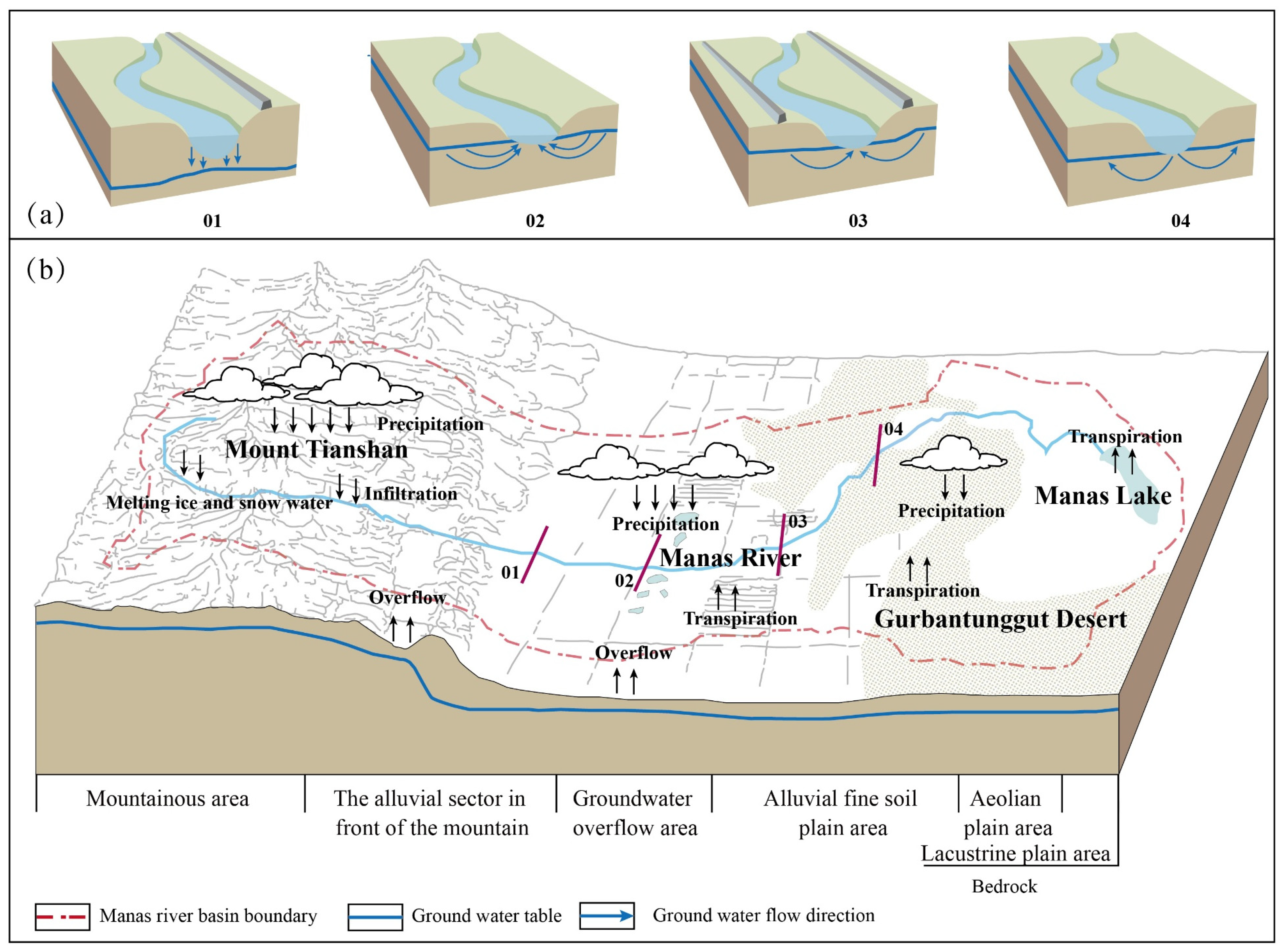
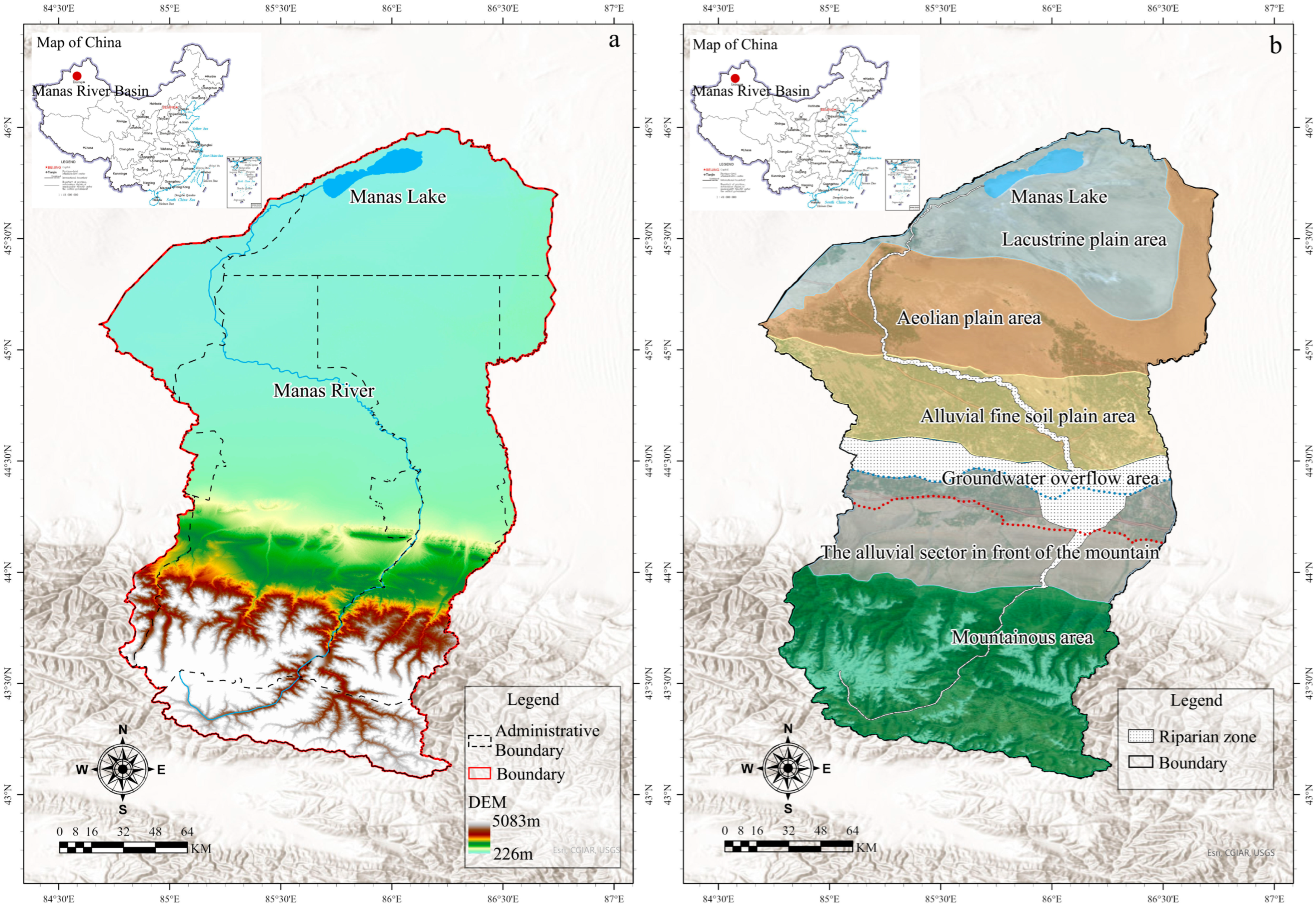
The Manas River Watershed is located on the northern slope of the Tianshan Mountains and the southern margin of the Junggar Watershed, covering an area of approximately 34,498.84 km². The northern boundary borders the Gurbantunggut Desert, one of China’s eight major deserts (Figure 1a). The watershed exhibits a typical “mountain–oasis–desert” geomorphological gradient. The upstream region is mainly recharged by snowmelt and glacial runoff; the midstream area contains concentrated oases, agricultural zones, and urban settlements; and the downstream area features a flat topography, intense evaporation, and a fragile ecological environment. Following the landscape–hydrological framework proposed by Wang et al. [31] from the perspective of “river–groundwater transformation” in arid regions, the Manas River Watershed was divided longitudinally into six typical geomorphological–hydrological subregions: mountain zone, piedmont alluvial fan zone, groundwater overflow zone, fine alluvial plain zone, aeolian plain zone, and lacustrine plain zone. Within each subregion, riparian zone boundaries were determined based on geomorphic and hydrological characteristics: 50 m in width in the mountainous, aeolian, and lacustrine plain zones; 500 m in the fine alluvial plain zone; while the alluvial fan zone was delineated according to fan morphology. The groundwater overflow zone, characterized by extensive lakes and close hydraulic connectivity between riverbanks and lake shores, was entirely included in the riparian system (Figure 1b). The delineation of riparian zones was based on a combination of geomorphological and hydrological criteria. Geomorphologically, the boundaries were determined by topography and surface ecological conditions along the upstream–downstream gradient; hydrologically, they were influenced by groundwater outflow and shallow burial zones, adjusted according to local drainage networks. The total riparian zone area was defined as 2603.99 km².

From the piedmont alluvial fan to the downstream aeolian plain, the interaction between surface water and groundwater displays pronounced spatial heterogeneity (Figure 2b), which can be generalized into four typical patterns (Figure 2a): Disconnection–infiltration recharge in the alluvial fan zone: The gravelly aquifers have high permeability, causing riverbeds to dry up during low-flow periods and substantial infiltration recharge during floods, forming a “disconnected” pattern (Figure 2a-01). Groundwater-fed rivers in the overflow zone: Finer sediments reduce permeability, groundwater depth ranges from 0–3 m, and spring outflow occurs at gullies. The right bank continuously recharges the river, while the left bank may experience backflow during high water levels. Overextraction in recent years has reduced spring discharge by over 60% (Figure 2a-02). Alternating recharge and discharge in the alluvial plain: Multilayer aquifer systems experience strong human interference from irrigation and groundwater pumping. During dry seasons, rivers recharge aquifers; during floods, infiltration from canals and floods replenish shallow groundwater (<5 m) (Figure 2a-03). Seasonal infiltration recharge in the aeolian plain: Fine sandy aquifers have low permeability, with groundwater buried at 5–10 m depth. Recharge occurs only during artificial water transfer periods. In the right-bank desert area, weak human interference leads to relatively stable water tables (Figure 2a-04).

2.2. Data Sources

This study uses five sets of land-use data (2000, 2005, 2010, 2015, and 2020) obtained from the Resource and Environmental Science Data Center of the Chinese Academy of Sciences (RESDC, https://www.resdc.cn) with a spatial resolution of 30 m × 30 m [32]. The elevation data (DEM) were derived from the SRTM 30 m dataset provided by RESDC. Meteorological data, including annual precipitation and mean annual temperature, were collected from 8 national meteorological stations within and surrounding the watershed. These point data were interpolated into a 30 m spatial resolution using the Kriging method to ensure spatial consistency. Soil texture and type data (1:1,000,000) and NDVI data (Normalized Difference Vegetation Index) were also acquired from RESDC. Socio-economic data were obtained from the Resource and Environmental Science Data Center of the Chinese Academy of Sciences (RESDC) and local statistical yearbooks. Specifically, the socio-economic variables included gridded GDP density and population density datasets with an original spatial resolution of 1 km × 1 km, which were resampled to 30 m × 30 m to ensure consistency with the land-use datasets. Given that 8 stations represent an average density of approximately one station per 4312 km² across the ~34,499 km² watershed, the resulting kriged surfaces should be understood as spatially smooth first-order estimates of regional climatic gradients rather than fine-scale validated precipitation fields. Interpretations of precipitation (X₅) as a GeoDetector driving variable are accordingly limited to broad spatial trends. It should be noted that this resampling does not generate new spatial information at the 30-m scale; the effective spatial resolution of these socio-economic variables remains 1 km × 1 km, and all interpretations of their driving effects should be understood at that resolution. In addition, county-level statistical data on cultivated land area and total agricultural output value were collected from the Xinjiang Statistical Yearbook and local county statistical bulletins for the corresponding study years. These variables were used to characterize the intensity of agricultural development and socio-economic activities across the watershed. All spatial datasets were standardized to a unified 30 m resolution using GIS. Hydrological data underpinning the RGT pattern delineation and groundwater level variable (X₄) were synthesized from multiple sources: (1) published peer-reviewed studies on RGT dynamics in the Manas River Watershed [31,33]; (2) the systematic regional groundwater survey and environmental assessment of the Junggar Basin, providing basin-scale aquifer characterization and multi-decade water table records; (3) the watershed-level groundwater resource survey and evaluation report, supplying zone-differentiated groundwater depth, recharge rates, and discharge estimates across the six geomorphological subregions; and (4) multi-year field investigations and direct measurements conducted by the research team in the Manas River Watershed, including field surveys of riparian zone hydrological conditions, groundwater depth observations at representative transects, and on-site verification of RGT zone boundaries. Collectively, these sources provide the empirical foundation for the RGT spatial framework applied in this study. It should nonetheless be noted that a continuous piezometric monitoring network covering the full 2000–2020 study period was not deployed as part of this study, and the groundwater level variable used in GeoDetector represents a synthesized spatial estimate rather than a temporally continuous measured field.

2.3. Methods

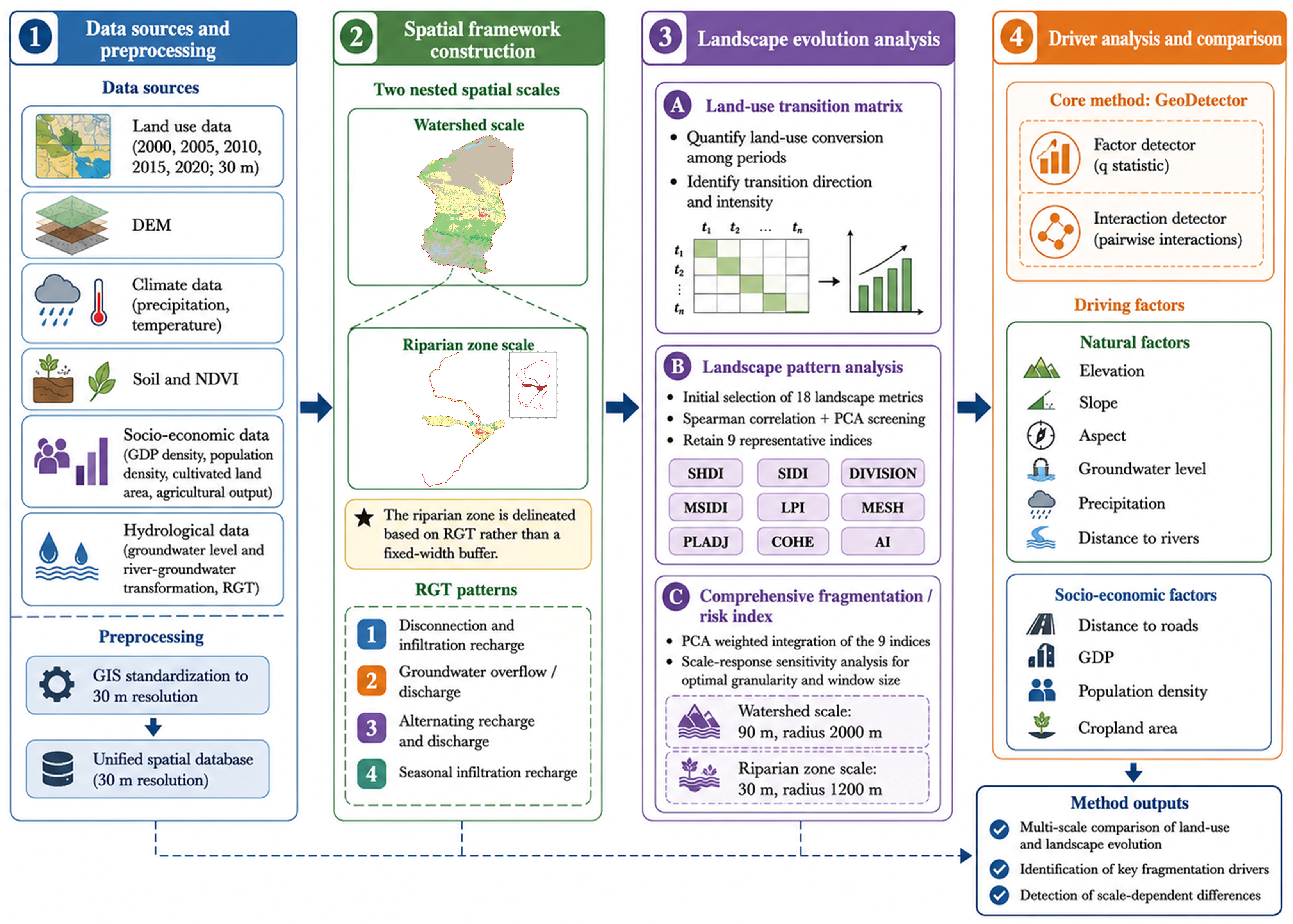
The methodological framework of this study is shown in Figure 3, integrating data preprocessing, spatial framework construction, landscape evolution analysis, and driving mechanism identification into a unified workflow. First, multi-source datasets were collected and standardized to build a spatial database at the watershed and riparian zone scales. Second, land-use transition matrices and landscape pattern indices (FRAGSTATS v2015; http://www.geodetector.cn/; accessed on 15 April 2026) were applied to quantify land-use change and landscape evolution, and principal component analysis (PCA) was used to construct a comprehensive fragmentation risk index. Finally, GeoDetector was employed to identify the effects of natural and socio-economic drivers and their interactions, followed by a multi-scale comparative analysis to reveal scale-dependent differences in landscape fragmentation and evolution.

2.3.1. Land-Use Transition Matrix

The land-use transition matrix quantitatively describes conversions among land-use types between two time periods, revealing the structure and functional transitions of land use in the watershed [34]. It identifies dominant transformation directions and rates, providing a quantitative basis for subsequent analysis of landscape pattern changes. The general matrix form is:

$$S_{ij=}\left(\begin{array}{cccc}{S}_{11}& S_{12}& \dots & S_{1n}\\ S_{21}& S_{22}& \dots & S_{2n}\\ ⋮& ⋮& \ddots & ⋮\\ S_{n1}& S_{n2}& \dots & S_{nn}\end{array}\right)$$

(1)

In the formula, S represents the area, n is the number of land use types, and i, j (i, j = 1, 2 …, n) respectively represent the land use types before and after the transfer, and $S_{ij}$ indicates the area of land type i that was converted to land type j before the transfer. Each column element in the matrix represents the flow information of the i-class before the transfer to the local classes after the transfer, and each row element in the matrix represents the source information of the j-class area after the transfer from the local classes before the transfer.

2.3.2. Landscape Types and Indices

(1) Spatial Distribution of Landscape Types

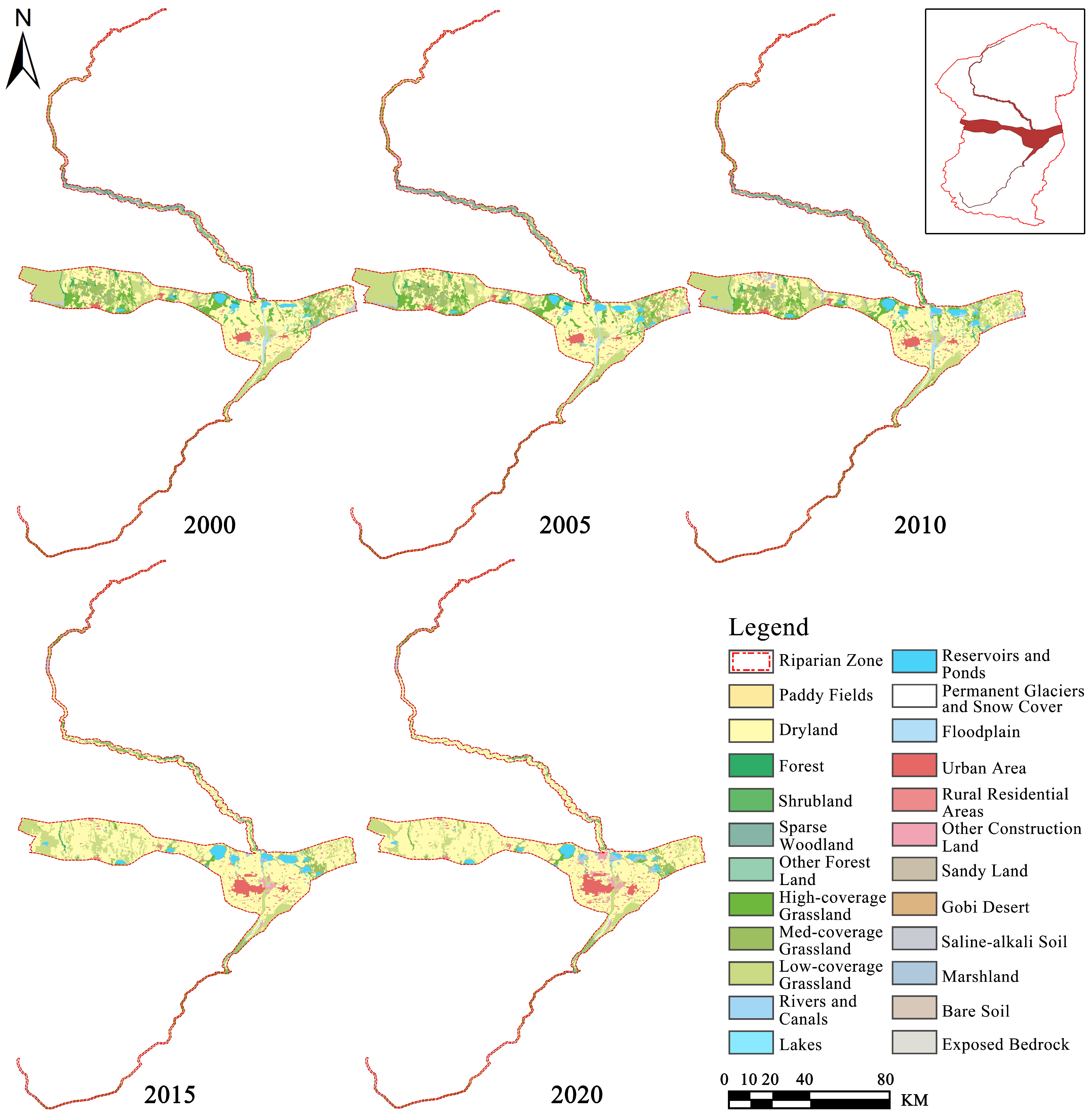
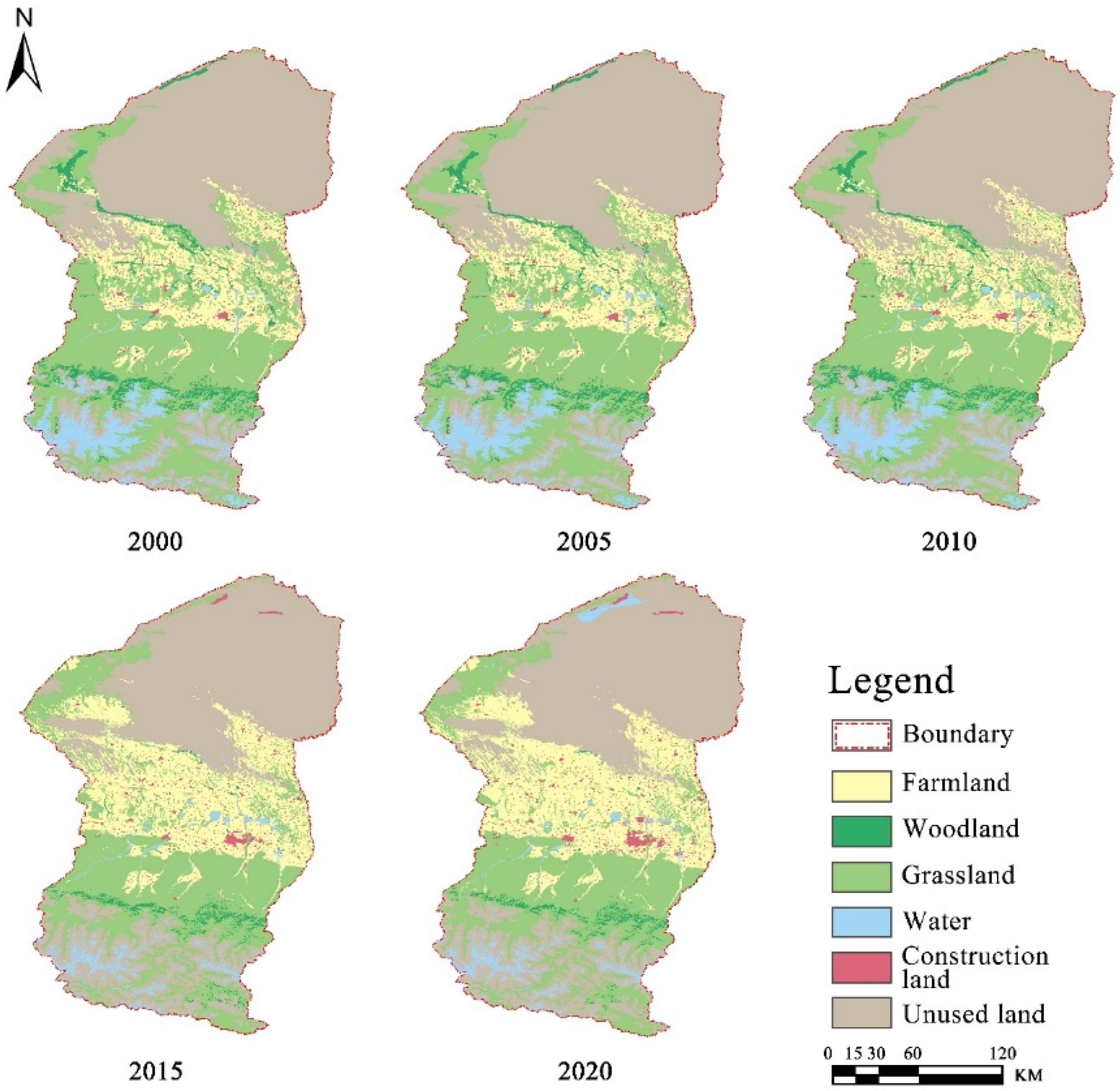
The classification system used in this study follows the two-level land-use scheme jointly developed by the Chinese Academy of Sciences and the Ministry of Agriculture: six primary types (cropland, forest, grassland, water, built-up land, and unused land) and 25 secondary categories (Table S1). As shown in Figure 4, land-use distribution in the Manas River Watershed is shaped by topography, soil, and socio-economic conditions. Cropland is mainly concentrated around towns and villages in plains; forestland is distributed in mountainous areas with minimal human disturbance; water bodies consist of rivers, reservoirs, and ponds; built-up land is sparsely distributed around towns and roads; and unused land occurs mainly in high-altitude mountain and desert areas, including exposed rock from glacial retreat and extensive Gobi deserts.

In the riparian zones (Figure 5), land use shows clear spatial differentiation. Cropland (dryland and paddy fields) is banded along rivers and irrigation canals, particularly in alluvial plains and floodplains near reservoirs. Forestland exhibits a vertical gradient—dense forests occur in groundwater overflow zones, shrubs along terraces, and grassland transitions between them. Built-up land is clustered along riverbanks and roads, while artificial water bodies are embedded between cropland and settlements. Upstream is dominated by bare rock, transitioning downstream into Gobi Desert mixed with saline-alkali soils and seasonal wetlands.

(2) Selection of Landscape Pattern Indices

Landscape indices quantitatively characterize landscape composition and spatial configuration [2]. Based on prior research and watershed characteristics, 18 metrics were initially considered. After Spearman correlation testing and principal component analysis, nine representative indices were retained: Shannon’s Diversity Index (SHDI), Simpson’s Diversity Index (SIDI), Landscape Division Index (DIVISION), Modified Shannon’s Diversity Index (MSIDI), Largest Patch Index (LPI), Effective Mesh Size (MESH), Percentage of Like Adjacencies (PLADJ), Patch Cohesion Index (COHE), and Aggregation Index (AI). Their definitions and ecological interpretations are listed in Table S2 of the Supplementary Materials.

2.3.3. Methodology for Landscape Fragmentation Driver Analysis

(1) Comprehensive Landscape Index

To comprehensively capture fragmentation, the nine selected indices were linearly combined using principal component weights to construct a composite fragmentation index. This integration reduces redundancy while highlighting major fragmentation trends across time and space.

(2) GeoDetector Analysis

The GeoDetector method identifies spatial heterogeneity and quantifies the driving forces of geographical phenomena [35]. It includes four modules, of which the factor detector and interaction detector were used here to explore natural and socio-economic drivers of multi-scale landscape evolution.

1) Factor detector: The factor detector examines whether a certain geographical factor is the cause of the spatial differentiation of a certain geographical feature and the extent to which it can explain that differentiation. The magnitude of the q value can represent the explanatory power of the driving factor on the dependent variable, and its expression is:

$$q=1-{\displaystyle \frac{{\sum }_{h=1}^L{N}_h{\sigma }_h^2}{N{\sigma }^2}}$$

(2)

where L is the number of strata of factor X, $N_h$ and $N$ represent the number of samples in layer h and the whole region, respectively; ${\sigma }_h^2$ and ${\sigma }^2$ are the variances of the dependent variable Y in layer h and the entire study area. A larger q value indicates stronger explanatory power.

2) Interaction detector: Interaction detection is used to identify the interactions between different factors X and evaluate whether the combined effect of two factors will increase or decrease the explanatory power for variable Y. The types of interactions between two factors are shown in the formula:

Nonlinear weakening:

q(X1 ∩ X2) < Min(q(X1), q(X2))

(3)

Single-factor weakening:

Min(q(X1), q(X2)) < q(X1 ∩ X2) < Max(q(X1), q(X2))

(4)

Bivariate enhancement:

q(X1 ∩ X2) > Max(q(X1), q(X2))

(5)

Independent:

q(X1 ∩ X2) = q(X1) + q(X2)

(6)

Nonlinear enhancement:

q(X1 ∩ X2) > q(X1) + q(X2)

(7)

In the formula: q(X1) and q(X2) respectively represent the influence of the factors X1 and X2; q(X1 ∩ X2) represents the influence of the interaction between factors X1 and X2.

3. Results

3.1. Characteristics of Land Use Change

3.1.1. Watershed Scale Land Use Change

Between 2000 and 2020, the Manas River Watershed underwent significant land-use transformation, characterized by the rapid expansion of cropland and built-up land and the continuous decline of ecological land (

Table 1. Land-use areas and their percentage changes at the watershed scale.

Year	2000 (km2)	2005 (km2)	2010 (km2)	2015 (km2)	2020 (km2)	Change % (2000–2005)	Change % (2005–2010)	Change % (2010–2015)	Change % (2015–2020)	Total Change % (2000–2020)
Farmland	4452.45	4903.08	7208.76	7303.66	7668.43	+10.12%	+47.03%	+1.32%	+5.00%	+72.23%
Woodland	1273.19	1248.02	494.65	494.88	452.17	−1.98%	−60.37%	+0.05%	−8.63%	−64.48%
Grassland	10,970.79	10,605.45	10,015.95	9935.98	9579.27	−3.33%	−5.56%	−0.80%	−3.59%	−12.68%
Water	2147.63	2130.15	947.71	952.53	1062.19	−0.81%	−55.51%	+0.51%	+11.51%	−50.54%
Construction land	321.51	350.90	441.13	503.16	541.02	+9.14%	+25.71%	+14.06%	+7.52%	+68.27%
Unused land	15,333.28	15,261.07	15,390.89	15,308.79	15,196.07	−0.47%	+0.85%	−0.53%	−0.74%	−0.90%

). From 2000 to 2010, agricultural expansion and urbanization were dominant. Cropland increased by 2756 km², accounting for 85.7% of the total 20-year increment, mainly converted from grassland and forestland. Built-up land increased by 119.6 km² (54.5% of total growth), reflecting simultaneous agricultural and urban expansion—an “oasis-type expansion based on agriculture” development model. Meanwhile, ecological land shrank sharply: forestland decreased by 778.5 km², grassland by 954.8 km² (95.5 km²/year on average), and water areas declined by 55.9%, suggesting intensified human pressure on natural landscapes. During 2010–2020, the watershed entered a period of structural stabilization. Although cropland continued to expand (net increase of 459.7 km²), the rate slowed considerably. Built-up land increased by 100 km², concentrated in midstream urban or county such as Shihezi City and Manas County. This indicates a trend toward spatial intensification and agglomeration. Simultaneously, water bodies slightly recovered but remained below 2000 levels, while forest and grassland degradation slowed. Overall, the Manas River Watershed followed a trajectory of “rapid expansion—partial recovery—structural stabilization.”

3.1.2. Riparian Zone Scale Land Use Change

Land-use transitions in the riparian zones were even more intense and concentrated than those at the watershed scale (

Table 2. Land use areas and their percentage changes in the riparian zones.

Year	2000 (km2)	2005 (km2)	2010 (km2)	2015 (km2)	2020 (km2)	Change % (2000–2005)	Change % (2005–2010)	Change % (2010–2015)	Change % (2015–2020)	Total Change % (2000–2020)
Paddy Fields	-	0.21	8.52	10.12	10.84	-	+3957.1%	+18.8%	+7.1%	-
Dryland	1019.98	1057.07	1551.46	1552.16	1655.36	+3.6%	+46.8%	+0.05%	+6.6%	+62.3%
Forest	41.78	41.46	5.70	5.69	0.17	−0.8%	−86.3%	−0.2%	−97.0%	−99.6%
Shrubland	0.82	0.82	14.30	14.32	11.24	0.0%	+1643.9%	+0.1%	−21.5%	+1270.7%
Sparse Woodland	114.40	106.53	4.01	4.03	3.71	−6.9%	−96.2%	+0.5%	−7.9%	−96.8%
Other Forest Land	10.36	10.35	6.57	7.03	6.16	−0.1%	−36.5%	+7.0%	−12.4%	−40.5%
High-coverage Grassland	209.77	205.59	63.49	89.66	66.94	−2.0%	−69.1%	+41.2%	−25.3%	−68.1%
Med-coverage Grassland	247.40	246.39	163.50	156.26	135.02	−0.4%	−33.6%	−4.4%	−13.6%	−45.4%
Low-coverage Grassland	610.32	582.13	418.89	402.37	309.44	−4.6%	−28.0%	−3.9%	−23.1%	−49.3%
Rivers and Canals	-	-	16.32	16.08	16.23	-	-	−1.5%	+0.9%	-
Lakes	1.76	1.79	1.25	0.93	0.91	+1.7%	−30.2%	−25.6%	−2.2%	−48.3%
Reservoirs and Ponds	74.00	46.32	101.51	53.12	67.33	−37.4%	+119.1%	−47.7%	+26.8%	−9.0%
Permanent Glaciers and Snow Cover	3.35	3.36	1.45	1.44	1.46	+0.3%	−56.8%	−0.7%	+1.4%	−56.4%
Flood plain	36.25	42.06	16.94	16.37	16.28	+16.0%	−59.7%	−3.4%	−0.6%	−55.1%
Urban Area	46.31	63.99	72.14	97.03	86.84	+38.2%	+12.7%	+34.5%	−10.5%	+87.5%
Rural Residential Areas	48.77	47.83	59.04	59.09	65.38	−1.9%	+23.4%	+0.1%	+10.6%	+34.1%
Other Construction Land	4.49	4.50	19.02	19.60	47.81	+0.2%	+322.7%	+3.1%	+143.9%	+964.8%
Sandy Land	14.70	14.39	12.23	12.12	11.39	−2.1%	−15.0%	−0.9%	−6.0%	−22.5%
Gobi Desert	19.89	19.89	22.35	22.36	22.15	0.0%	+12.4%	+0.04%	−0.9%	+11.4%
Saline-alkali Soil	81.93	76.95	1.13	1.12	1.04	−6.1%	−98.5%	−0.9%	−7.1%	−98.7%
Marshland	13.86	28.51	24.24	33.07	48.44	+105.7%	−15.0%	+36.4%	+46.5%	+249.5%
Bare Soil	-	-	0.03	10.12	0.01	-	-	+33,633%	−99.9%	-
Exposed Bedrock	3.72	3.72	19.84	19.84	19.84	0.0%	+433.3%	0.0%	0.0%	+433.3%

). Between 2000 and 2020, dryland cropland expanded significantly by 635.4 km², 77.8% of which occurred between 2005 and 2010—reflecting a peak in agricultural intensification. Built-up land increased by 87.5%, with 79.2% of growth during 2010–2020, indicating accelerated urban and infrastructural concentration along rivers. In contrast, ecological land suffered substantial losses: forestland nearly disappeared (−99.6%), mainly between 2005 and 2010; high-coverage grassland declined by 68.1%, with over 70% of losses before 2010.

Water systems showed fluctuating shrinkage: reservoir and pond areas decreased by 27.7 km² between 2000 and 2005, rebounded in 2010 due to artificial water supplementation, and declined again by 33.7% by 2020. Overall, the period 2005–2015 marked the critical stage of riparian land transformation—rapid expansion of cropland and construction land, continued ecological degradation, and a transition from natural/semi-natural to human-dominated landscapes. The expansion of agricultural and urban land along riverbanks substantially altered surface cover and weakened the buffering and infiltration capacity of riparian ecosystems, demonstrating their high sensitivity to human disturbance and hydrological changes.

3.2. Spatial and Temporal Variations in Landscape Pattern Indices

3.2.1. Watershed Scale Landscape Indices

Against the backdrop of significant land-use transformation, the landscape pattern of the Manas River Watershed exhibited multi-stage, cross-scale evolution (

Table 3. Landscape pattern indices at the watershed scale.

Year	SHDI	SIDI	DIVISION	MSIDI	LPI	MESH	PLADJ	COHESION	AI
2000	1.27	0.62	0.65	0.98	55.97	2,735,959.47	94.97	99.43	95.18
2005	0.51	0.21	0.21	0.24	88.48	23,555,720.25	98.59	99.60	98.67
2010	1.24	0.62	0.66	0.98	55.97	2,704,006.06	94.87	99.43	95.07
2015	0.81	0.38	0.39	0.47	77.88	9,588,626.92	97.40	99.52	97.53
2020	1.28	0.68	0.83	1.13	30.44	582,322.84	89.13	99.41	89.42

). In 2000, high SHDI and SIDI values coupled with low LPI indicated high diversity and no single dominant patch type. In 2005, SHDI plummeted (0.51), while LPI and MESH increased sharply—suggesting large-scale expansion of homogeneous patches and a dramatic drop in diversity. By 2010, SHDI (1.24) and SIDI (0.62) rebounded to near-2000 levels, with declining LPI and MESH, indicating temporary recovery of diversity and mitigation of fragmentation. In 2015, index values reflected transitional adjustments, while by 2020, SHDI (1.28) and SIDI (0.68) reached peak values, LPI fell to 30.44, and DIVISION rose significantly, implying increased patch complexity and intensified fragmentation. Overall, the watershed-level landscape evolved through a process of “diversity decline—temporary recovery—intensified fragmentation.”

3.2.2. Riparian Zone Scale Landscape Indices

At the riparian zone scale, landscape evolution exhibited a higher spatial sensitivity to human activities (

Table 4. Landscape pattern indices at the riparian zone scale.

Year	SHDI	SIDI	DIVISION	MSIDI	LPI	MESH	PLADJ	COHESION	AI
2000	1.91	0.77	0.96	1.47	12.55	9838.10	93.60	99.00	93.95
2005	1.90	0.77	0.96	1.45	12.00	9406.52	93.42	98.93	93.78
2010	1.52	0.61	0.95	0.95	11.82	12,102.79	93.79	99.07	94.12
2015	1.55	0.61	0.95	0.95	10.99	11,977.80	93.74	99.08	94.08
2020	1.48	0.58	0.94	0.86	12.56	15,844.71	94.09	99.15	94.41

). From 2000 to 2005, SHDI and SIDI remained stable, with minor decreases in LPI and MESH, suggesting limited disturbance. Between 2010 and 2015, SHDI and SIDI declined, while MESH increased and DIVISION decreased, accompanied by rising PLADJ and AI values. This reflected expanding agricultural and construction patches with improved connectivity. By 2020, SHDI and SIDI reached their lowest levels, LPI increased to 12.56, and MESH peaked, indicating dominance of several large, homogeneous patches. Although DIVISION decreased, its relatively high value suggested persistent micro-fragmentation within large patches (Such as ditch cutting). Overall, riparian zones underwent a compound evolution of “diversity loss—patch enlargement—enhanced connectivity.” Human activities along river corridors expanded agricultural and infrastructural land, improving spatial continuity but intensifying ecological homogenization and micro-fragmentation—highlighting the vulnerability of riparian zones as transitional interfaces between natural and human systems.

3.3. Identification and Analysis of Driving Factors for Landscape Fragmentation

3.3.1. Comprehensive Landscape Risk Index

To assess overall fragmentation, a comprehensive landscape index LRI (Landscape Risk Index) was constructed from nine core metrics (SHDI, SIDI, DIVISION, MSIDI, LPI, MESH, PLADJ, COHE, AI) using weighted principal components:

LRI = 0.2079 × SHDI + 0.2899 × SIDI + 0.2071 × DIVISION + 0.2897 × MSIDI − 0.123 × LPI − 0.167 × MESH − 0.065 × PLADJ + 0.208 × COHESION + 0.203 × AI

(8)

This index can reduce the redundancy of indicators while highlighting the main characteristics of landscape fragmentation changes. To enhance the spatial representativeness and robustness of the analysis, this study determined the optimal analysis granularity and amplitude through a preliminary scale-response sensitivity analysis across a gradient from 500 m to 5000 m. For the watershed scale, a granularity of 90 m and an analysis window radius of 2000 m were utilized, as this radius was identified as the characteristic ‘inflection point’ where the variance of key landscape metrics (e.g., SHDI and AI) stabilized. This setting is large enough to encompass the average size of major irrigation blocks in the oasis while preventing the over-smoothing of spatial heterogeneity. Conversely, for the riparian zone, a 30 m scale and a 1200 m window radius were selected to align with the lateral extent of river–groundwater influence zones identified in the RGT patterns. This dual-scale setting, while taking into account both micro-landscape details (such as ditch cutting) and overall stability, ensures comparability across spatial scales and provides a unified, robust framework for quantifying fragmentation and subsequent driver identification.

3.3.2. Coupling Ecological Risk with RGT Patterns

The following analysis is based on spatial overlay of landscape risk hotspots (derived from surface land-use and landscape metrics) with the RGT zone boundaries established through multi-source hydrogeological data [31,33] and field verification by the research team. The associations identified are spatial and correlative in nature; they do not constitute direct continuous monitoring of groundwater dynamics or vadose zone processes during the 2000–2020 study period.

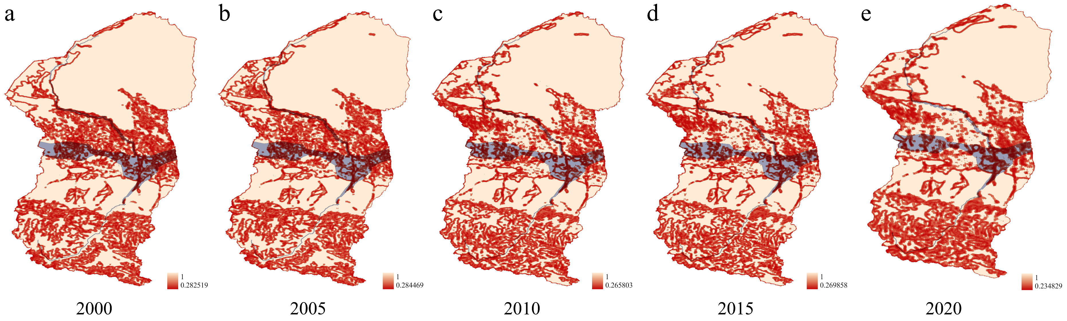
Figure 6 illustrates the spatio-temporal dynamics of landscape risk hotspots from 2000 to 2020. Qualitatively, the maps reveal a progressive expansion and intensification of high-risk clusters (indicated in dark red) primarily within the central and southern parts of the watershed. In 2000, high-risk areas were relatively fragmented and confined to existing oasis edges. However, by 2010 and continuing through 2020, these hotspots significantly coalesced into broad, continuous bands, reflecting a transition from isolated disturbance to systematic landscape degradation.

By performing a spatial overlay analysis between these risk hotspots (Figure 6a–e) and the RGT patterns (Figure 2a), a critical spatial coupling emerges:

(1) The Groundwater Overflow Zone (Pattern 02): This area exhibits the highest density and most rapid expansion of high-risk hotspots. The spatial intersection shows that a significant majority of the expanded high-risk clusters are situated within this zone. The qualitative shift from light pink to dark red across the time panels (2000–2020) is spatially consistent with the hypothesis that intensive groundwater extraction and agricultural encroachment have disrupted the natural spring discharge mechanism—a process documented across multiple hydrogeological datasets [31,33] and corroborated by regional survey data; as well as field observations by the research team—suggesting that this zone may have transitioned from a ‘hydrological source’ to an ‘ecological risk sink.’ The precise magnitude and temporal dynamics of this transition require further verification through a dedicated long-term monitoring network.

(2) The Disconnection Zone (Pattern 01): In contrast, the upstream alluvial fan maintains a consistently lower risk level (indicated by lighter tones), indicating that the landscape structure here remains relatively intact. Preserving the vertical infiltration capacity in this zone is critical for maintaining regional hydrological security.

(3) The Fine Alluvial and Aeolian Plains: The panels for 2015 and 2020 show a noticeable ‘finger-like’ expansion of risk into the northern plains, geographically coinciding with the extension of irrigation canals and the fragmentation of natural desert vegetation.

3.3.3. GeoDetector Driver Analysis

Based on previous research [21], to explore the driving mechanism of landscape fragmentation, classified by natural and social factors, Ten driving factors were selected and categorized as natural or socio-economic (

Table 5. Driving factors for landscape evolution in the Manas River Watershed.

Category	Dimension	Variable Code	Indicator	Unit
Natural Factors	Topography & Landform	X1	Elevation	m
		X2	Slope	°
		X3	Aspect	°
	Groundwater	X4	Groundwater Level	m
	Precipitation	X5	Precipitation	mm
	Ecological Barrier	X6	Distance to River	km
Social Factors	Anthropogenic Barrier	X7	Distance to Road	km
	Economy	X8	GDP	10,000 yuan
	Population	X9	Population Density	people/km2
	Irrigation Area	X10	Farm Land Area	km2

): elevation (X₁), slope (X₂), aspect (X₃), groundwater level (X₄), precipitation (X₅), distance to rivers (X₆), distance to roads (X₇), GDP (X₈), population density (X₉), and cropland area (X₁₀).

(1) Factor Detector Results

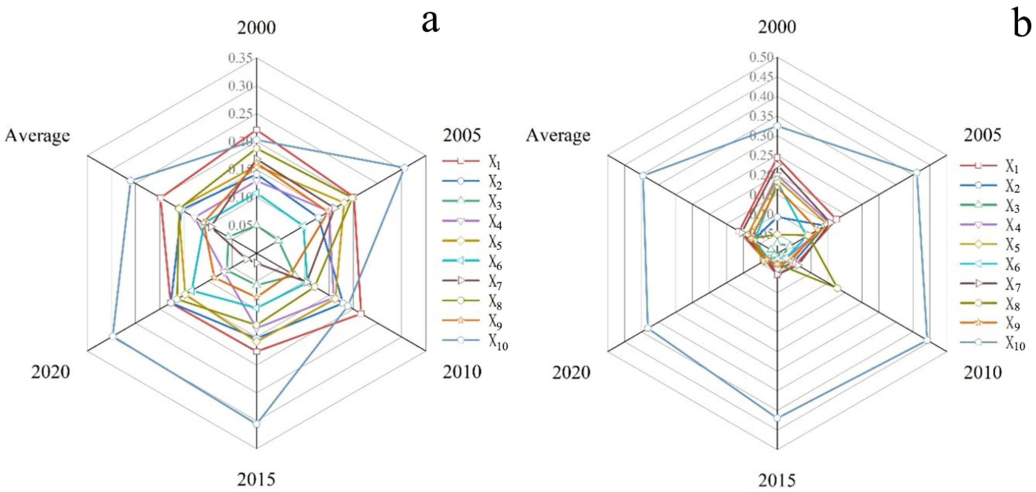
GeoDetector results (

Table 6. Factor detector results for watershed-scale drivers.

	X1	X2	X3	X4	X5	X6	X7	X8	X9	X10
2000	0.2210	0.1418	0.0497	0.1298	0.1570	0.1079	0.1687	0.1879	0.1614	0.2030
2005	0.2015	0.1278	0.0453	0.1500	0.181	0.0970	0.1614	0.1982	0.1481	0.3060
2010	0.2164	0.1786	0.0793	0.1593	0.1629	0.1051	0.1035	0.1201	0.0714	0.1890
2015	0.1760	0.1526	0.0572	0.1343	0.1583	0.0980	0.0177	0.1287	0.0789	0.3061
2020	0.1778	0.1769	0.0610	0.0670	0.1473	0.1339	0.0211	0.1642	0.0873	0.2974
Average	0.1985	0.1555	0.0585	0.1281	0.1613	0.1084	0.0945	0.1598	0.1094	0.2603

) indicate that from 2000 to 2020, the driving mechanism of landscape fragmentation transitioned from natural to human dominance. In 2000, elevation (X₁) and precipitation (X₅) were the strongest drivers (q = 0.1985 and 0.1613), implying geomorphological and climatic control. It should be noted that the precipitation layer was interpolated from 8 meteorological stations, which constrains the spatial precision of this variable; its explanatory power in GeoDetector should therefore be interpreted as representing broad climatic zonation rather than fine-scale rainfall heterogeneity. Distance to rivers (X₆) and groundwater level (X₄) also played important roles (q > 0.12), highlighting hydrological constraints.

Between 2005 and 2010, the explanatory power of cropland area (X₁₀) and GDP (X₈) increased rapidly to 0.2974 and 0.1621, respectively—signaling agricultural expansion and economic growth as emerging dominant forces. Concurrently, the influence of groundwater and precipitation declined by 57.5% and 85.3%, reflecting the weakening of natural hydrological connectivity due to irrigation and groundwater exploitation.

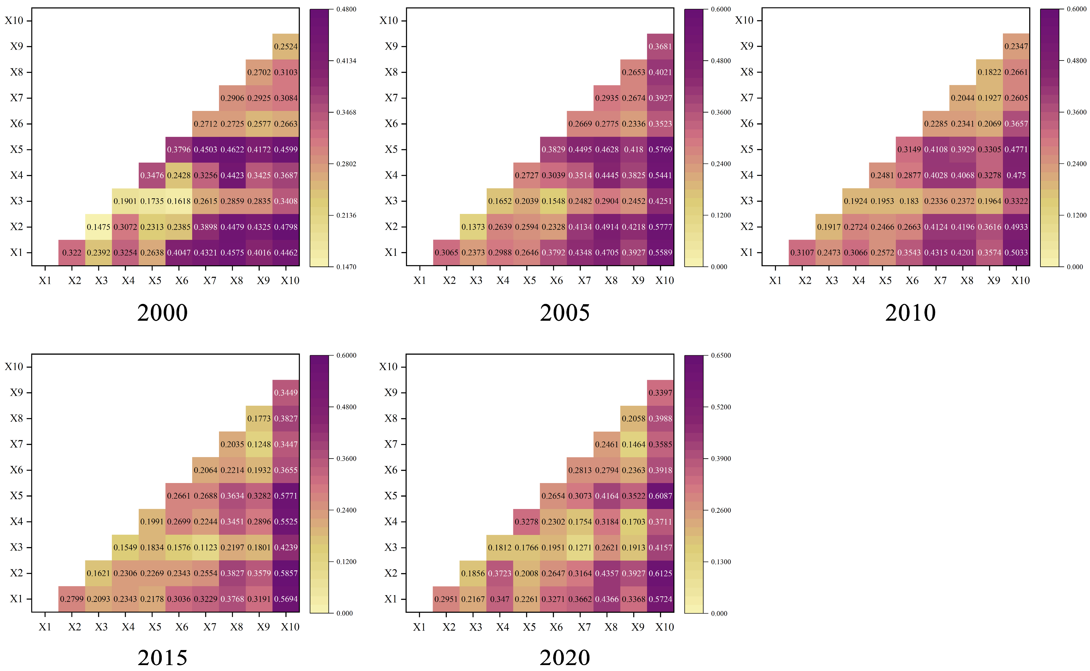
After 2010, socio-economic factors fully replaced natural ones. Cropland area (X₁₀) remained the most influential (mean q = 0.3957), and proximity to transportation corridors (X₇) gained importance after 2015, indicating that infrastructure upgrades and spatial clustering reshaped landscape structures (Figure 6a).

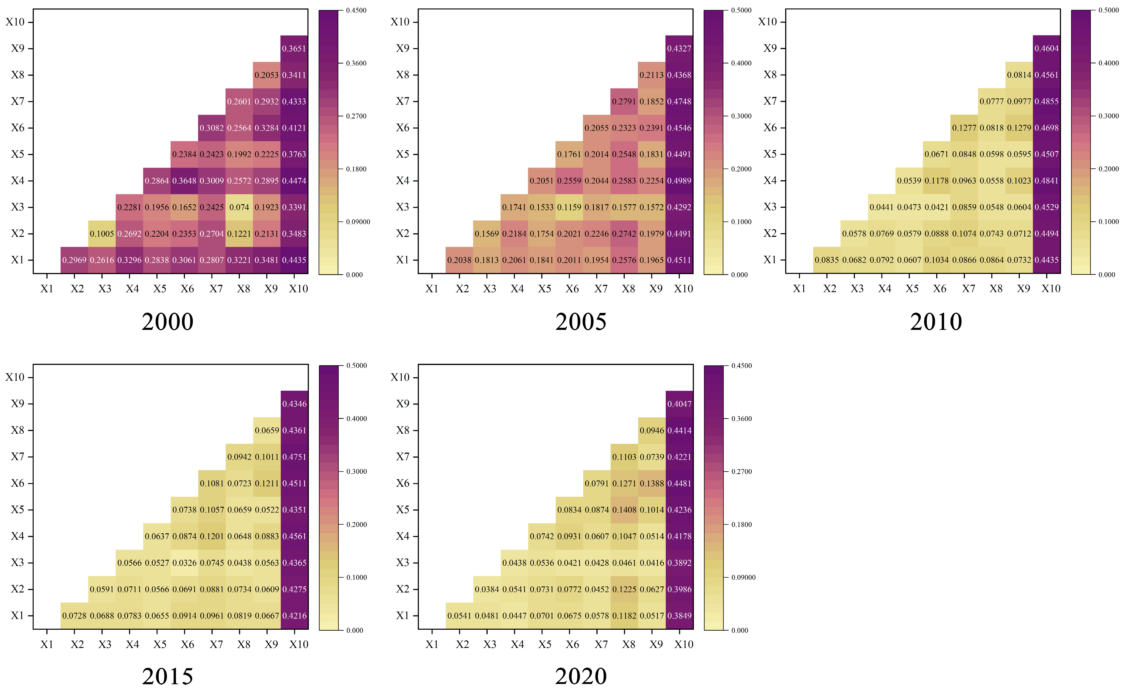
At the riparian zone scale (

Table 7. Factor detector results for riparian-scale drivers.

	X1	X2	X3	X4	X5	X6	X7	X8	X9	X10
2000	0.2438	0.0926	0.0259	0.1996	0.1884	0.1814	0.2254	0.0484	0.1684	0.3246
2005	0.1738	0.1412	0.0368	0.1540	0.1473	0.0868	0.1563	0.0917	0.1191	0.4111
2010	0.0553	0.0468	0.0132	0.0252	0.0337	0.0248	0.0609	0.1775	0.0397	0.4418
2015	0.0554	0.0403	0.0088	0.0345	0.0400	0.015	0.0538	0.0266	0.0274	0.4196
2020	0.0356	0.0261	0.0079	0.0292	0.0378	0.0267	0.0297	0.0373	0.0306	0.3815
Average	0.1128	0.0694	0.0185	0.0885	0.0894	0.0669	0.1052	0.0763	0.0770	0.3957

), this trend was even more pronounced. The explanatory power of elevation (X₁) dropped sharply from 0.2438 to 0.0356, while cropland area and GDP remained dominant, revealing the extreme sensitivity of riparian landscape fragmentation to agricultural and economic activities. This transition demonstrates a shift from a “naturally constrained” to a “human-dominated” mechanism, with hydrological conditions evolving from primary constraints to responsive variables (Figure 7b).

(2) Interaction Detector Results

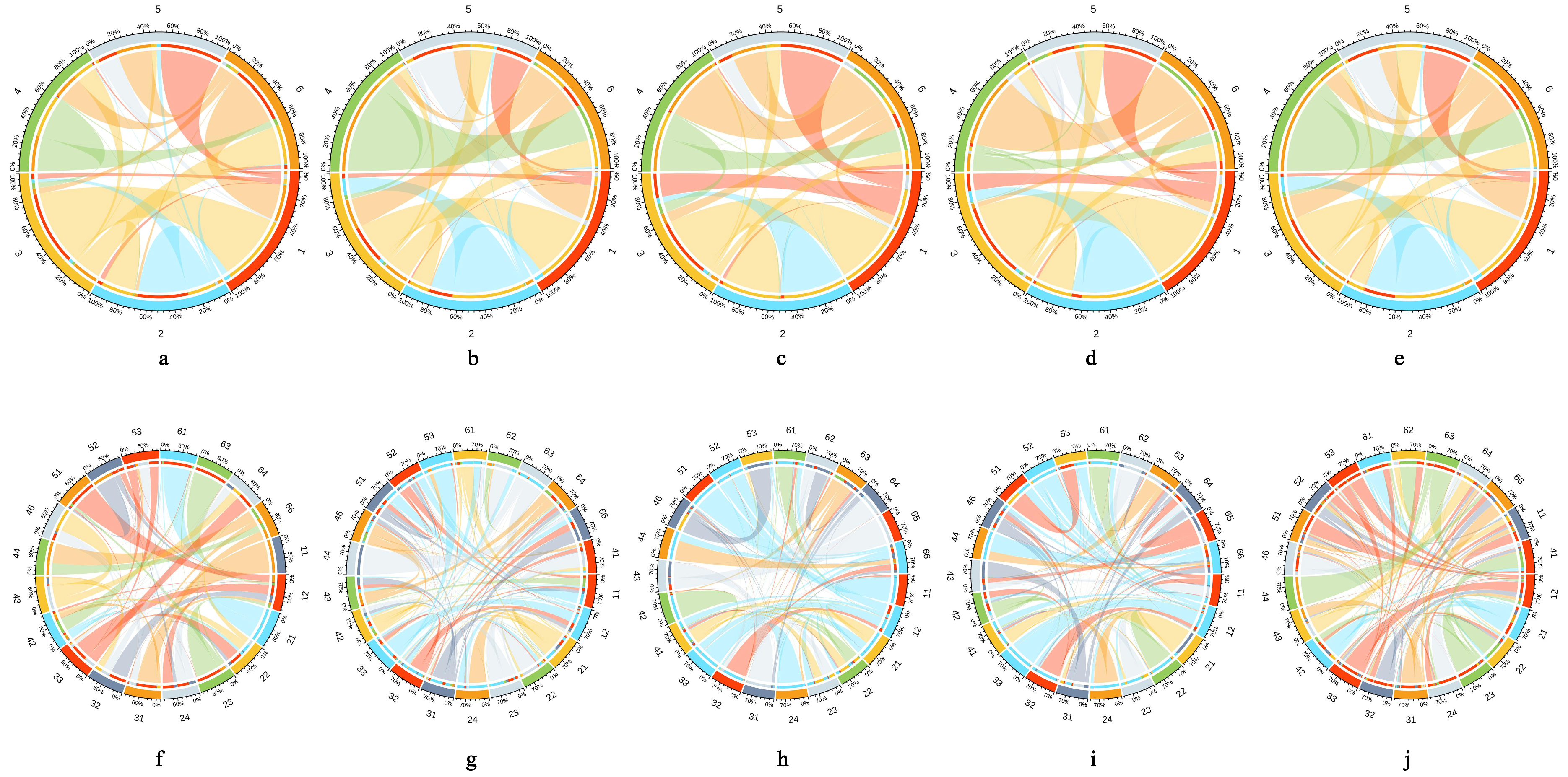
Interaction analysis (Figure 8 and Figure 9) further reveals the composite mechanisms underlying landscape evolution. Between 2000 and 2020, the watershed’s driving forces evolved from “natural dominance” to “natural–socioeconomic synergy” and finally to “socioeconomic dominance.” In 2000, interactions between topography and groundwater were strongest (q > 0.25), reflecting the leading role of physical geography. By 2005, interactions between cropland area, slope, and GDP strengthened, marking rapid socio-economic influence. In 2010, natural and human factors were nearly balanced, reflecting improved water use efficiency and precision agriculture. After 2015, socio-economic factors fully dominated—interactions between cropland and GDP peaked, illustrating the coupling of agricultural intensification and economic growth. By 2020, cropland–precipitation and cropland–slope interactions were most significant (q > 0.4), indicating deep integration of water-saving agriculture with terrain–hydrology constraints.

At the riparian scale, the evolution followed a “natural–social–technological–governance” sequence. From 2000–2005, natural hydrological factors dominated; 2005–2010 saw strengthened interactions between economic activities and road networks; 2010–2015 marked peak interactions between cropland and transport corridors; and 2015–2020 represented a “regulation and governance” phase characterized by water-saving and restoration policies. Overall, landscape fragmentation evolved from natural to socio-economic control, and finally to co-regulation by human activities and governance, reflecting a transition from resource exploitation to ecological restoration in arid inland watersheds.

4. Discussion

4.1. Stage Characteristics and Spatial Differentiation of Land Use Change

To better understand the spatial and temporal patterns of land-use evolution in the Manas River Watershed, this section synthesizes multi-period analysis results (Figure 10). Overall, land use in the watershed experienced a typical three-stage trajectory between 2000 and 2020, rapid expansion–partial recovery–structural stabilization, accompanied by significant spatial differentiation.

The period from 2000 to 2010 was a time of intense reshaping of the land use pattern at the watershed scale. This decade marked an intensive phase of agricultural expansion and urbanization. Large areas of unused and forested land were converted into cropland, forming an extended “oasis expansion belt” along rivers and irrigation networks. This period coincided with Xinjiang’s agricultural modernization and large-scale water diversion projects, reinforcing a “water-determined cultivation” pattern [36,37,38]. Simultaneous growth of cropland and built-up land reflected the spatial concentration of economic activities around water sources, laying the foundation for subsequent landscape restructuring.

From 2010 to 2015, the land use pattern of the watershed entered an adjustment stage at the watershed scale. Excessive agricultural and urban expansion in the previous stage caused both water stress and ecological degradation. As a result, national and regional policies—such as Grain for Green, wetland restoration, and ecological water replenishment—were implemented, shifting land use from extensive expansion to internal optimization. Cropland growth slowed, and some areas reverted to forest or grassland. Water areas partially recovered around the periphery of irrigation districts. Spatially, land-use changes concentrated in midstream oasis margins and groundwater overflow zones, forming “cropland–grassland–forestland” transition belts. This period signified a transition from resource-driven to ecologically constrained development, establishing an initial balance between exploitation and protection.

After 2015, the land use pattern in the watershed entered a stage of structural reorganization and stabilization. As the regional economy transformed and spatial planning improved, land use exhibited greater intensification and functional differentiation. Cropland growth decelerated; built-up land became more concentrated around towns and transport corridors, forming compact spatial clusters. Concurrently, ecological water supplementation and wetland restoration expanded water areas by ~12%, reduced fragmentation, and improved connectivity. Ecological recovery occurred mainly in downstream plains and saline flats, while upstream efforts focused on water-saving agriculture and canal optimization. The overall pattern evolved toward “stable agriculture, clustered urbanization, and ecological recovery,” indicating a shift from unregulated expansion to regulated, restoration-oriented equilibrium.

At the riparian scale, land-use transformation was more concentrated and intense, peaking between 2005 and 2015 (Figure 10). Construction and agriculture expanded rapidly along rivers and transport corridors, leading to large-scale conversion of ecological land (≈43% loss of forest and grassland). Since riparian zones are the main interfaces of surface–groundwater exchange, such transformations not only altered surface cover but also disrupted infiltration, flood retention, and ecological buffering [22]. This structural disturbance to hydrological processes reveals the key vulnerable links of the riparian zone in the watershed landscape system. Overall, the intensity of land conversion and irreversible ecological loss in the riparian zone are significantly higher than those in the watershed, reflecting its high vulnerability to human interference. This differentiation pattern reveals the multi-scale response characteristics of land use evolution, providing a basis for further exploration of the driving mechanism and response process of landscape pattern evolution (see Section 4.2).

4.2. Multi-Scale Driving Forces of Landscape Evolution

During the long-term evolution of land use transformation, the changes in the landscape pattern of the Manas River Watershed reflect the dynamic game between natural constraints and socio-economic disturbances. The results of geographical exploration show that the driving factors of landscape fragmentation exhibit significant differences in both time and scale, presenting a phased evolution trend of “nature dominance—the synergy of nature and social economy—social economy dominance”.

At the watershed scale, natural factors controlled landscape evolution during 2000–2010, consistent with Li et al. [21]. Topography, groundwater, and precipitation governed ecological spatial differentiation [39,40], while human influence was limited. From 2010 to 2015, agricultural intensification and infrastructure expansion increased the explanatory power of socio-economic variables, showing co-regulation between natural and human processes. Water diversion and canal construction enhanced irrigation efficiency but weakened natural hydrological connectivity [41], leading to simultaneous cropland expansion and ecological contraction. After 2015, landscape change entered a human-dominated stage. Cropland and urban areas continued to expand, and economic and transportation factors became primary drivers. Landscape fragmentation and ecological degradation intensified, revealing human activity as the central force behind spatial restructuring.

At the riparian scale, landscape response was more abrupt and localized. From 2000 to 2010, hydrological and geomorphological processes maintained longitudinal “mountain–oasis–desert” gradients and ecological connectivity. During 2010–2015, canal construction and irrigation expansion are associated with landscape changes in river–groundwater interaction zones [31], with surface land-use patterns consistent with reduced lateral connectivity—a trend also reflected in the declining spring discharge documented in regional hydrogeological surveys. Whether these surface changes directly caused subsurface hydrological disconnection at specific locations requires independent long-term groundwater monitoring to confirm at the process level. After 2015, policy interventions became the dominant force. Ecological water replenishment, Grain for Green, and wetland restoration projects led to partial recovery of water and vegetation [37], gradually improving landscape diversity and connectivity. Nevertheless, riparian zones remain tension zones between ecological restoration and agricultural productivity, with landscape patterns evolving through cycles of recovery–disturbance–rebalancing.

Overall, landscape evolution in the Manas River Watershed illustrates a triadic “nature–society–policy” coupling characteristic of arid inland watersheds. Natural processes establish the spatial foundation; human activities amplify disturbances; and policy interventions act as feedback regulators guiding restoration and equilibrium [20,40,42]. Topography and hydrology shape the landscape base, socio-economic forces modify its structure, and governance feedback steers it toward balance. Consequently, at the watershed level, fragmentation is the dominant feature, while at the riparian level, structural homogenization and ecological fragility prevail—together forming a nested socio-ecological system.

4.3. Hydro-Spatial Governance: Zoning Based on River–Groundwater Transformations

Over recent decades, human-induced land-use changes have become the major force reshaping landscape patterns [43,44], significantly influencing runoff, evapotranspiration, vegetation diversity, and hydrological cycles [45,46]. Consequently, the evolution of landscape patterns in arid watersheds has shifted from being nature-dominated to human-dominated, posing new challenges for ecological security and spatial governance. Although ecological redline zoning—based on ecosystem sensitivity and service value—has improved regional ecological security [47,48], single-scale or purely engineering approaches often fail to address system-level fragmentation and functional degradation [49,50]. Thus, watershed governance in arid regions must transition from structural restoration to systemic regulation, building an integrated governance framework that combines natural constraints, socio-economic regulation, and policy instruments.

This study found that, at the watershed scale, landscape pattern evolution was initially dominated by natural factors such as elevation and precipitation, but gradually came under the influence of socioeconomic drivers. The combined effects of cropland expansion and economic growth significantly promoted landscape homogenization, while road construction and hydraulic engineering intensified the fragmentation and functional degradation of ecological spaces. At the riparian zone scale, construction activities have expanded along transportation corridors and urban nodes, occupying groundwater recharge areas and disrupting the connectivity between rivers and aquifers. This has further amplified ecological risks and fragmentation trends. At the watershed scale, the overall landscape structure is primarily shaped by while riparian zones, through their spatial continuity, reveal finer-scale internal dynamics—together forming a nested social–ecological system. Based on these findings, this study proposes a multi-scale spatial governance optimization framework for the Manas River Watershed, centered on hierarchical and zoned management, eco-hydrological coupling regulation, and policy integration.

(1) Hierarchical and Zoned Spatial Governance

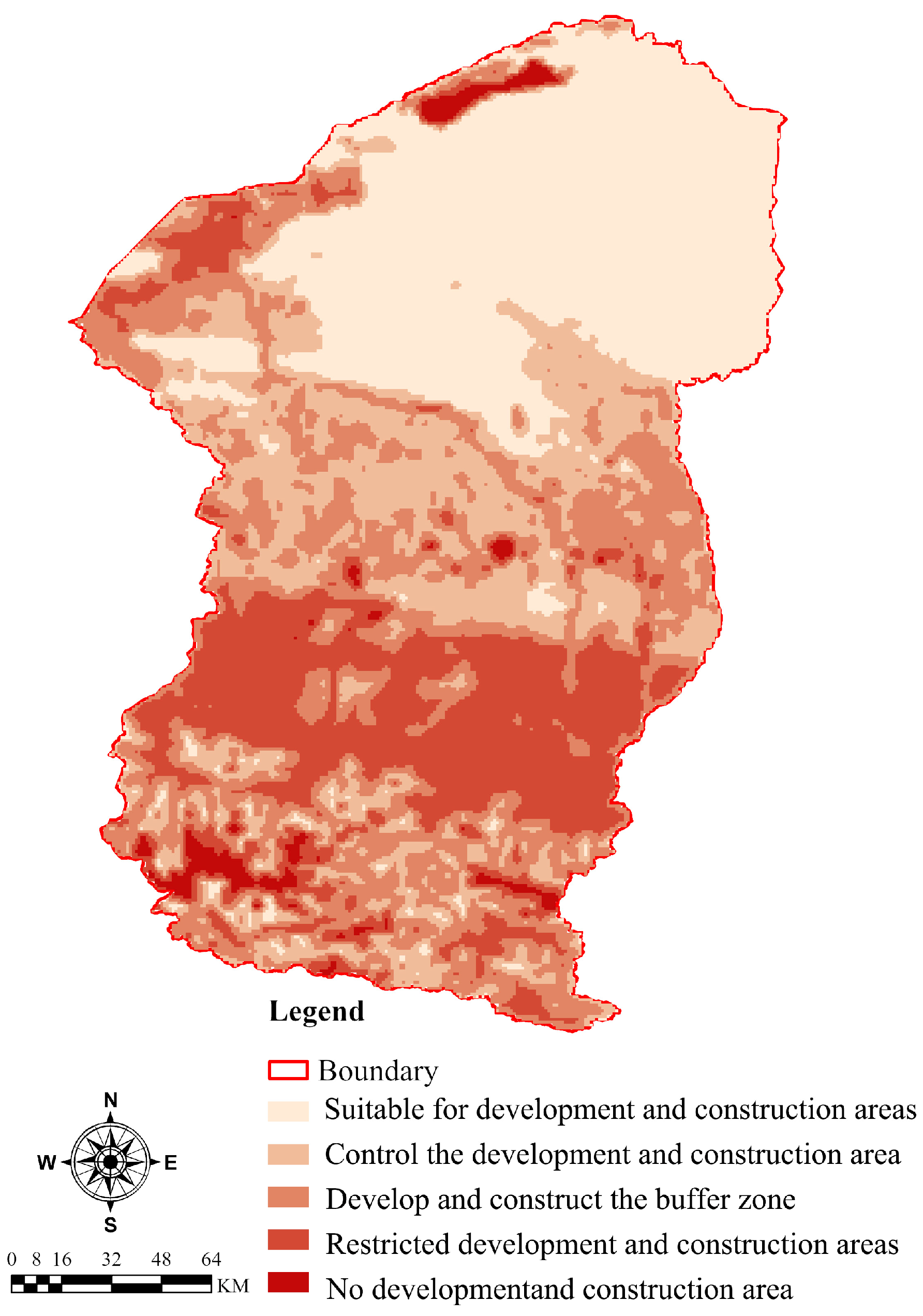
The goal of hierarchical and zoned governance is to manage watershed space by considering ecological sensitivity, water resource carrying capacity, and land-use suitability, achieving refined regulation under the principle of “clear boundaries, defined responsibilities” [51,52,53]. At the watershed scale, five spatial management zones can be delineated (Figure 11): Strict Protection Zone: Located at the foothills of the Tianshan Mountains and major headwater areas, focusing on restoring native vegetation and river–groundwater interfaces, removing artificial embankments, and maintaining hydrological connectivity. Restricted Use Zone: Mainly covering riparian zones and oasis edges, designed to build grass–shrub buffer belts, control desertification, and maintain ecological stability in transition zones. Buffer Zone: Surrounding irrigated areas, where water-saving agriculture, crop rotation, and land consolidation are applied to control cropland expansion. Moderate Use Zone: Focused on optimizing agricultural structure, promoting efficient irrigation, and encouraging ecological farmland transformation. Key Development Zone: Concentrated around existing urban centers and transport corridors, aiming to enhance land-use efficiency through compact development.

(2) Constructing the “Four Zones, Three Belts, and One Corridor” Spatial Pattern

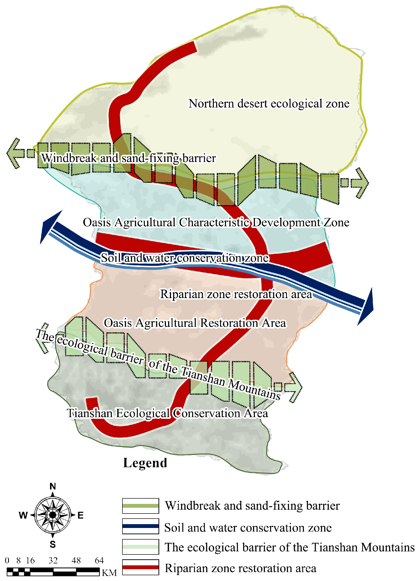
At the zoning level, a three-tier spatial pattern— “Four Zones, Three Belts, and One Corridor” (Figure 12)—is proposed, with ecological security as the foundation, agricultural sustainability as the core, and spatial coordination as the guiding principle. Four Zones: The northern desert ecological zone, the oasis agricultural development zone, the agricultural restoration zone, and the Tianshan ecological conservation zone. These zones correspond to distinct ecological functions, forming a gradient system of protection–utilization–restoration–conservation. Three Belts: A windbreak–sand fixation belt, a soil–water conservation belt, and a mountain-foot ecological barrier belt. Together, they form an ecological security shield for the watershed and enhance energy and material flow buffering capacity. One Corridor: The river ecological corridor, linking upstream and downstream as well as both riverbanks, restoring longitudinal hydrological connectivity and lateral ecological migration pathways to strengthen watershed-wide ecological integrity.

This spatial structure integrates ecological restoration, agricultural production, and urban–rural development, providing a spatial foundation for the coordinated evolution of ecological, economic, and social systems.

(3) Policy-Oriented Systemic Governance and Implementation Mechanisms

Driven by policy orientation and institutional innovation, systemic governance is shifting from single-factor control to integrated multi-mechanism coordination. The combination of ecological compensation, water rights adjustment, and dynamic assessment mechanisms reflects both the horizontal transfer of ecosystem service values and enhanced cooperation among stakeholders [54]. In practice, horizontal ecological compensation systems based on the “upstream supply–downstream benefit” relationship have been widely adopted [55] Under China’s Ecological Protection Compensation Regulation [56], compensation through financial transfers and industrial collaboration ensures alignment between responsibilities and benefits, improving long-term policy effectiveness. Meanwhile, a market-based tradable water rights system, defined by groundwater depth and ecological water demand thresholds, regulates resource allocation and encourages water-saving practices. Furthermore, an ecological health dynamic assessment system, combining landscape metrics with remote sensing and GIS technologies, provides quantitative and feedback-based scientific support for policy implementation. This aligns with the human–land system coupling modeling concept proposed by Khan et al. [57], enabling bidirectional feedback between policy responses and ecological risks. A pertinent example of such a system is demonstrated in the research by Sabljić et al. [58], who utilized Sentinel-2 and Landsat data to monitor land degradation and deforestation caused by mining activities in Bosnia and Herzegovina. Their findings emphasize that identifying spatial changes through advanced remote sensing techniques is fundamental for sustainable land-use planning and the restoration of degraded ecosystems. Similarly, in the Manas River Watershed, our use of RGT-based landscape risk hotspots provides a precise spatial basis for adaptive governance, allowing for a balance between industrial/agricultural development and environmental health. We emphasize that the RGT-landscape risk coupling presented here is grounded in multi-source hydrogeological evidence (peer-reviewed studies, regional government survey reports, and team field measurements) but remains a spatially corroborated inference rather than the output of a fully coupled surface–subsurface model. The governance recommendations are best understood as evidence-informed, spatially targeted priorities for intervention, to be further validated through dedicated long-term piezometric monitoring and physically-based hydrological modeling. Through mechanism complementarity and policy coordination, systemic governance is evolving into a compound pattern characterized by compatible incentives and adaptive dynamics [59], achieving a sustainable balance between ecological protection and regional development.

Beyond northwestern China, similar landscape evolution trajectories have been widely documented in arid and semi-arid river basins worldwide, suggesting that the socio-hydrological mechanisms identified in the Manas River Watershed may have broader applicability. In the western United States, irrigation intensification has substantially reduced streamflow sustainability and altered riparian ecological functions, demonstrating how agricultural expansion can amplify hydrological stress and reshape watershed resilience [60]. Likewise, large-scale dam construction in the United States has fragmented river systems and reversed natural connectivity patterns, fundamentally transforming watershed structure and ecological integrity [61]. Similar degradation processes have also been observed in floodplain systems, where human interventions have weakened hydrological connectivity and reduced landscape integrity [62].

Compared with these international cases, the Manas River Watershed exhibits a distinct hydro-ecological characteristic: the strong dependence of riparian landscape evolution on river–groundwater transformation (RGT) patterns. While previous international studies mainly emphasize surface-water regulation or infrastructure fragmentation, our findings highlight that subsurface hydrological connectivity is equally critical in shaping landscape heterogeneity and ecological stability. This suggests that effective spatial governance in arid watersheds should move beyond conventional buffer-based planning toward hydro-spatial governance frameworks that explicitly integrate vertical groundwater dynamics. Such an approach may provide transferable planning insights for other inland arid basins facing agricultural expansion, groundwater depletion, and ecological degradation.

4.4. Limitations and Future Prospects

Although this study reveals the dual-scale characteristics and driving forces of landscape evolution in the Manas River Watershed, several limitations remain:

First, regarding the delineation of riparian zones, this study improved upon the traditional “uniform buffer width” approach by adopting a fixed-width classification by subregion. However, hydrological dynamics—such as flood peaks and groundwater fluctuations—were not fully considered. Future work should develop hydrologically driven, ecologically responsive dynamic boundary models [63] that adjust automatically with changes in water levels and channel morphology, integrating flow monitoring, groundwater depth, and geomorphic features. A primary limitation of this study concerns the nature of the surface–subsurface hydrological linkage. While the groundwater component draws on a multi-source empirical foundation—including published hydrogeological studies [31,33], the regional groundwater resource survey, the watershed-specific planning assessment, and multi-year field investigations by the research team—this study does not include a continuous piezometric monitoring network, vadose zone instrumentation, or a coupled surface–subsurface model calibrated specifically to the 2000–2020 study period. Consequently, the ecological risk patterns identified in Section 3.3.2 characterize surface landscape conditions within zones whose groundwater regimes are empirically established, and the surface–subsurface linkage is best described as an empirically informed spatial inference rather than a mechanistically demonstrated process. Future research should integrate dedicated long-term piezometric networks, stable isotope tracing, and physically based coupled models (e.g., MODFLOW-SWAT) to move from spatial corroboration to mechanistic quantification of these linkages.

Second, in terms of data precision and spatial resolution, this study used 30 m Landsat imagery, adequately represents watershed-scale landscape dynamics but cannot capture small features (<10 m²) such as shrub patches, aquatic vegetation, or micro-wetlands within riparian zones. Future research should integrate high-resolution imagery (e.g., Sentinel-2, GF-6, or multispectral UAV data) with field sampling to achieve finer spatiotemporal characterization of landscape and hydrological processes [64] Similarly, the kriging-based interpolation of precipitation from 8 stations across a ~34,499 km² watershed introduces significant uncertainty in characterizing elevation-driven precipitation gradients—particularly in the transition from the Tianshan Mountain zone to the piedmont alluvial fan and desert plain. Future work should incorporate CHIRPS, ERA5-Land, or GPM IMERG gridded precipitation products, validated against station data, to improve spatial representativeness of climatic drivers.

Third, regarding driving mechanism modeling and process interpretation, this study employed the GeoDetector method to reveal spatial–temporal variations in the influence of natural and human factors, yet did not establish a clear process coupling mechanism. Furthermore, to overcome the limitations of the current statistical driving analysis, future research should transition toward deeper process-based coupling. Specifically, the integration of the InVEST–Water Yield model with System Dynamics (SD) modeling presents a promising pathway. The InVEST model can quantify the spatial distribution of water-related ecosystem services under different land-use scenarios, while the SD model can simulate the temporal feedback mechanisms and policy-driven trajectories of the human–land system. By coupling these two approaches, researchers can better reveal the complex spatial–temporal variations in how natural factors (e.g., precipitation and evaporation) and human factors (e.g., irrigation policy and urbanization) interact to influence watershed ecological health. Additionally, incorporating ecosystem service valuation [65] and multi-objective optimization algorithms [66] could help identify critical thresholds and trade-offs in landscape evolution, providing quantitative support for systematic watershed management in arid regions.

Fourth, the spatial resolution mismatch among driving variables represents an additional analytical constraint. While land-use and landscape metrics were derived from 30-m Landsat imagery, key socio-economic drivers—specifically GDP density (X₈) and population density (X₉)—were originally available only at 1 km × 1 km resolution and were resampled to 30 m for geometric consistency. This disaggregation introduces artificial spatial precision: the GeoDetector analysis of these variables reflects 1-km scale patterns, not genuine 30-m heterogeneity. Future studies should seek finer-resolution socio-economic proxies (e.g., nighttime light intensity, building footprint data, or point-of-interest density) to achieve true multi-scale correspondence between drivers and landscape responses.

5. Conclusions

Through multi-temporal land use and landscape pattern analysis (2000–2020), this study uncovered the processes, drivers, and socio-ecological contradictions of landscape evolution in the Manas River Watershed. The reorganized main conclusions are as follows:

(1) Phased patterns and hierarchical nesting of landscape systems: Landscape evolution followed a “rapid expansion–temporary recovery–stabilization” trajectory. Spatially, the system exhibits a nested structure: the watershed scale reflects overall macro-level fragmentation, while riparian zones act as highly sensitive focal areas exposing local ecological vulnerability and structural homogenization.

(2) Driving mechanisms shifted from nature-constrained to human-dominated: Prior to 2000, topography and hydrology were the primary spatial constraints. Post-2010, agricultural expansion, GDP growth, and infrastructure construction became overwhelmingly dominant, marking a fundamental transition to a “human activity-driven, natural process-responding” regime.

(3) Society–ecosystem interaction exhibits a ternary “nature–society–policy” coupling: The landscape evolves through a three-phase interaction: natural foundation, human amplification, and policy feedback. Policy measures (e.g., ecological water replenishment, wetland restoration) have become the critical regulatory mechanism, steering the watershed from “resource-driven development” toward “governance-driven restoration”.

(4) A novel “Hydro-Spatial” planning paradigm based on RGT patterns: Effective watershed governance requires moving beyond rigid administrative zoning to process-based zoning defined by hydrological connectivity (e.g., groundwater overflow limits). This paradigm relies on hierarchical zoning control, coupled eco-hydrological element regulation, and the embedding of market-based policy tools (e.g., water rights trading, ecological compensation) to shift from engineering-based to systemic governance.

Ultimately, landscape evolution in arid watersheds is not a linear natural degradation process but a dynamic reorganization of the social–ecological–policy system. Future spatial governance must emphasize integrity, ecological security, and water coordination, advancing the paradigm shift from “development–restoration–rebalance” to “coexistence–regulation–resilience”.

References

1. Wu, J. Landscape sustainability science: Ecosystem services and human well-being in changing landscapes. Landsc. Ecol. 2013, 28, 999–1023. [Google Scholar] [CrossRef]
2. Deng, J.S.; Wang, K.; Hong, Y.; Qi, J.G. Spatio-temporal dynamics and evolution of land use change and landscape pattern in response to rapid urbanization. Landsc. Urban Plan. 2009, 92, 187–198. [Google Scholar] [CrossRef]
3. McGarigal, K.S.; Cushman, S.; Neel, M.; Ene, E. FRAGSTATS: Spatial Pattern Analysis Program for Categorical Maps; University of Massachusetts: Amherst, MA, USA, 2002. [Google Scholar]
4. Wu, C.; Gao, P.; Xu, R.; Mu, X.; Sun, W. Influence of landscape pattern changes on water conservation capacity: A case study in an arid/semiarid region of China. Ecol. Indic. 2024, 163, 112082. [Google Scholar] [CrossRef]
5. Liu, X.; Shen, Y. Quantification of the impacts of climate change and human agricultural activities on oasis water requirements in an arid region: A case study of the Heihe River basin, China. Earth Syst. Dynam. 2018, 9, 211–225. [Google Scholar] [CrossRef]
6. Liu, C.; Zhang, F.; Carl Johnson, V.; Duan, P.; Kung, H.-T. Spatio-temporal variation of oasis landscape pattern in arid area: Human or natural driving? Ecol. Indic. 2021, 125, 107495. [Google Scholar] [CrossRef]
7. Hayashi, M.; Rosenberry, D.O. Effects of Ground Water Exchange on the Hydrology and Ecology of Surface Water. Groundwater 2002, 40, 309–316. [Google Scholar] [CrossRef] [PubMed]
8. Chen, Q.; Li, Z.; Jin, Z.; Yao, S.; Zhou, Y.; Wu, H.; Liu, Y.; Zhang, G.; Liu, Y.; Yang, X.; et al. Evolution patterns, driving mechanisms, and ecological indicative effects of 730 lakes water color in the Yangtze River Basin (1984–2023). J. Hydrol. 2025, 653, 132695. [Google Scholar] [CrossRef]
9. Wang, W.; Gong, C.; Zhang, Z.; Chen, L. Research Status and Prospect of the Subsurface Hydrology and Ecological Effect in Arid Regions. Adv. Earth Sci. 2018, 33, 702–718. [Google Scholar]
10. Brunke, M.; Gonser, T. The ecological significance of exchange processes between rivers and groundwater. Freshw. Biol. 1997, 37, 1–33. [Google Scholar] [CrossRef]
11. Alley, W.M.; Healy, R.W.; LaBaugh, J.W.; Reilly, T.E. Flow and Storage in Groundwater Systems. Science 2002, 296, 1985–1990. [Google Scholar] [CrossRef]
12. Jasechko, S.; Seybold, H.; Perrone, D.; Fan, Y.; Kirchner, J.W. Widespread potential loss of streamflow into underlying aquifers across the USA. Nature 2021, 591, 391–395. [Google Scholar] [CrossRef] [PubMed]
13. Yao, Y.; Zheng, C.; Tian, Y.; Liu, J.; Zheng, Y. Numerical modeling of regional groundwater flow in the Heihe River Basin, China: Advances and new insights. Sci. China Earth Sci. 2015, 58, 3–15. [Google Scholar] [CrossRef]
14. Gregory, S.V.; Swanson, F.J.; McKee, W.A.; Cummins, K.W. An Ecosystem Perspective of Riparian Zones: Focus on links between land and water. BioScience 1991, 41, 540–551. [Google Scholar] [CrossRef]
15. Naiman, R.J.; Décamps, H. The Ecology of Interfaces: Riparian Zones. Annu. Rev. Ecol. Evol. Syst. 1997, 28, 621–658. [Google Scholar] [CrossRef]
16. Simon, A.; Collison, A.J. Quantifying the mechanical and hydrologic effects of riparian vegetation on streambank stability. Earth Surf. Process. Landf. 2002, 27, 527–546. [Google Scholar] [CrossRef]
17. Riis, T.; Kelly-Quinn, M.; Aguiar, F.C.; Manolaki, P.; Bruno, D.; Bejarano, M.D.; Clerici, N.; Fernandes, M.R.; Franco, J.C.; Pettit, N.; et al. Global Overview of Ecosystem Services Provided by Riparian Vegetation. BioScience 2020, 70, 501–514. [Google Scholar] [CrossRef]
18. Naiman, R.J.; Decamps, H.; Pollock, M. The Role of Riparian Corridors in Maintaining Regional Biodiversity. Ecol. Appl. 1993, 3, 209–212. [Google Scholar] [CrossRef]
19. Baudry, J.; Thenail, C. Interaction between farming systems, riparian zones, and landscape patterns: A case study in western France. Landsc. Urban Plan. 2004, 67, 121–129. [Google Scholar] [CrossRef]
20. Yan, Z.; Guo, Y.; Sun, B.; Gao, Z.; Qin, P.; Li, Y.; Yue, W.; Cui, H. Combating land degradation through human efforts: Ongoing challenges for sustainable development of global drylands. J. Environ. Manag. 2024, 354, 120254. [Google Scholar] [CrossRef]
21. Li, J.; Wang, J.; Du, Y.; Hou, X.; Xi, R.; Yang, Y. Assessing landscape fragmentation and its driving factors in arid regions: A case study of the Manas River, China. Ecol. Indic. 2025, 171, 113253. [Google Scholar] [CrossRef]
22. Wang, H.; Zhang, D.; Liu, S.; Ye, S.; Jin, X.; Wu, J. Regional proximity effects of landscape pattern evolution: Evidence from 325 county-level areas in the middle reaches of the Yangtze River, China. Sci. Total Environ. 2023, 903, 166134. [Google Scholar] [CrossRef]
23. Liu, J.; Xu, Q.; Yi, J.; Huang, X. Analysis of the heterogeneity of urban expansion landscape patterns and driving factors based on a combined Multi-Order Adjacency Index and Geodetector model. Ecol. Indic. 2022, 136, 108655. [Google Scholar] [CrossRef]
24. Zhang, X.; Liu, Y.; Zhou, L. Correlation Analysis between Landscape Metrics and Water Quality under Multiple Scales. Int. J. Environ. Res. Public Health 2018, 15, 1606. [Google Scholar] [CrossRef]
25. García-Ayllón, S.; Martínez, G. Analysis of Correlation between Anthropization Phenomena and Landscape Values of the Territory: A GIS Framework Based on Spatial Statistics. ISPRS Int. J. Geo-Inf. 2023, 12, 323. [Google Scholar] [CrossRef]
26. Zhang, J.; Zhang, Z.; Liu, L.; Cao, Y.; Zhang, M.; Yuan, Z.; Ma, R.; Liu, X.; Liu, Y. Scaling effects of ecosystem service trade-off and synergy in arid inland river basins: A case study of the Manas River Basin of Xinjiang, China. Ecol. Indic. 2025, 173, 113358. [Google Scholar] [CrossRef]
27. Qingqing, Z.; Hailiang, X.; Jingyi, F.; Pujia, Y.; Peng, Z. Spatial Analysis of Land Use and Land Cover Changes in Recent 30 Years in Manas River Basin. Procedia Environ. Sci. 2012, 12, 906–916. [Google Scholar] [CrossRef]
28. Zing, H.; Xu, H.; Qiao, M.; Fan, Z.; Shi, W.; Zhang, Q. Temporal-spatial Evolution of Stream Construction and Its Driving Forces in Manas River Basin During 1958–2006. Prog. Geogr. 2010, 29, 1129–1136. [Google Scholar] [CrossRef]
29. Wang, W.; Tian, H.; Yang, G.; Liu, B.; Pan, Y.; Ding, G.; Xu, X.; Dan, Y.; Cui, M.; Gao, Y. Dynamic variation of groundwater level and its influencing factors in typical oasis irrigated areas in Northwest China. Open Geosci. 2023, 15, 20220493. [Google Scholar] [CrossRef]
30. Wang, Z.H.; He, X.L.; Yang, G.; Li, S. Sustainable Strategies and Status of Unconventional Water Resources Development and Utilization in Manas River Basin. Adv. Mater. Res. 2010, 113–116, 565–570. [Google Scholar] [CrossRef]
31. Wang, J.; Ma, Z.; Wang, Z.; Huang, X.; Hou, Q.; Cao, Y.; Wang, W. Evolution of the landscape ecological pattern in arid riparian zones based on the perspective of watershed river-groundwater transformation. J. Hydrol. 2023, 625, 130119. [Google Scholar] [CrossRef]
32. Xu, X.; Liu, J.; Zhang, S.; Li, R.; Yan, C.; Wu, S. China national land use and land cover change remote sensing monitoring data set (CNLUCC) data registration and publication system of the data center for resources and environmental sciences. Chin. Acad. Sci. (RESDC) 2018. [Google Scholar] [CrossRef]
33. Hou, X. Study on Groundwater Environment Evolution and Regulation Mechanism in Manas River Basin under Changing Environment. Ph.D. Thesis, Chang’an University, Xi’an, China, 2023. [Google Scholar]
34. Chang, X.; Xing, Y.; Wang, J.; Yang, H.; Gong, W. Effects of land use and cover change (LUCC) on terrestrial carbon stocks in China between 2000 and 2018. Resour. Conserv. Recycl. 2022, 182, 106333. [Google Scholar] [CrossRef]
35. Wang, J.; Xu, C. Geodetector: Principle and prospective. Acta Geogr. Sin. 2017, 72, 116–134. [Google Scholar] [CrossRef]
36. Luo, M.; Liu, T.; Meng, F.; Duan, Y.; Bao, A.; Xing, W.; Feng, X.; De Maeyer, P.; Frankl, A. Identifying climate change impacts on water resources in Xinjiang, China. Sci. Total Environ. 2019, 676, 613–626. [Google Scholar] [CrossRef]
37. Pan, Y.; Tian, H.; Arsalan Farid, M.; He, X.; Heng, T.; Hermansen, C.; Wollesen de Jonge, L.; Li, F.; Gao, Y.; Tian, L.; et al. Metaheuristic optimization of water resources: A case study of the Manas River irrigation district. J. Hydrol. 2024, 639, 131640. [Google Scholar] [CrossRef]
38. Qin, J.; Tong, Y.; Farid, M.A.; Zhang, H.; Tian, H.; Li, X.; He, X.; Xue, L.; Li, Y.; Gao, Y.; et al. Multidimensional water-economic-ecological joint optimization for Manas River Basin, China, using a dual-population co-evolutionary algorithm. J. Hydrol. Reg. Stud. 2025, 60, 102465. [Google Scholar] [CrossRef]
39. Gao, Z.; Ye, J. Eco-environmental effects and differentiation mechanism of land use transition in Manas River Basin: A perspective based on the dominant function of “production-living-ecological” spaces. Arid. Land Geogr. 2024, 47, 1947–1956. [Google Scholar] [CrossRef]
40. Yang, F.; Deng, W.; Zhang, H.; Yuan, Q. Natural-human interactions impact wetland pattern evolution in different environment conditions in arid regions. J. Environ. Manag. 2025, 392, 126901. [Google Scholar] [CrossRef] [PubMed]
41. Hou, X.; Wang, W.; Wang, Z.; Ma, Z.; Guan, C.; Xi, D.; Li, P.; Li, J.; Huang, X. Hydrogeological processes and hydrochemical effects in the Manas river catchment, Northwest China, over the past 60 years. J. Hydrol. 2022, 614, 128338. [Google Scholar] [CrossRef]
42. Du, X.; Fang, Y.; Zhao, H.; Xu, X. Spatiotemporal evolution and driving forces of landscape structure and habitat quality in river corridors with ceased flow: A case study of the Yongding River corridor in Beijing, China. J. Environ. Manag. 2025, 374, 123861. [Google Scholar] [CrossRef]
43. Singh, S.K.; Srivastava, P.K.; Szabó, S.; Petropoulos, G.P.; Gupta, M.; Islam, T. Landscape transform and spatial metrics for mapping spatiotemporal land cover dynamics using Earth Observation data-sets. Geocarto Int. 2017, 32, 113–127. [Google Scholar] [CrossRef]
44. Forman, R.T.T.; Godron, M. Patches and Structural Components for A Landscape Ecology. BioScience 1981, 31, 733–740. [Google Scholar] [CrossRef]
45. Karlsen, R.H.; Bishop, K.; Grabs, T.; Ottosson-Löfvenius, M.; Laudon, H.; Seibert, J. The role of landscape properties, storage and evapotranspiration on variability in streamflow recessions in a boreal catchment. J. Hydrol. 2019, 570, 315–328. [Google Scholar] [CrossRef]
46. Han, Y.; Wang, J.-l.; Li, P. Influences of landscape pattern evolution on regional crop water requirements in regions of large-scale agricultural operations. J. Clean. Prod. 2021, 327, 129499. [Google Scholar] [CrossRef]
47. Mora, C.; Sale, P.F. Ongoing global biodiversity loss and the need to move beyond protected areas a review of the technical and practical shortcomings of protected areas on land and sea. Mar. Ecol. Prog. Ser. 2011, 434, 251–266. [Google Scholar] [CrossRef]
48. Wang, Y.; Pan, J. Establishment of ecological security patterns based on ecosystem services value reconstruction in an arid inland basin: A case study of the Ganzhou District, Zhangye City, Gansu Province. Acta Ecol. Sin. 2019, 39, 3455–3467. [Google Scholar] [CrossRef]
49. Pahl-Wostl, C.; Jeffrey, P.; Isendahl, N.; Brugnach, M. Maturing the New Water Management Paradigm: Progressing from Aspiration to Practice. Water Resour. Manag. 2011, 25, 837–856. [Google Scholar] [CrossRef]
50. Groot, J.C.J.; Yalew, S.G.; Rossing, W.A.H. Exploring ecosystem services trade-offs in agricultural landscapes with a multi-objective programming approach. Landsc. Urban Plan. 2018, 172, 29–36. [Google Scholar] [CrossRef]
51. Zhang, L.; Hou, Q.; Duan, Y. Governance pattern of basin ecological space in Loess Plateau of China. Trans. Chin. Soc. Agric. Eng. (Trans. CSAE) 2021, 37, 206–213, Chinese with English abstract. [Google Scholar] [CrossRef]
52. Liu, Y.; Zhou, Y. Territory spatial planning and national governance system in China. Land Use Policy 2021, 102, 105288. [Google Scholar] [CrossRef]
53. Zhang, C.; Wei, Z.; Shi, J.; Huang, Q.; Liu, F. Resilience-based zoning for sustainable cultivated land management: Integrating landscape morphology and environmental adaptability. J. Environ. Manag. 2025, 395, 127991. [Google Scholar] [CrossRef]
54. Osman, T.; Shaw, D.; Kenawy, E. Examining the extent to which stakeholder collaboration during ecotourism planning processes could be applied within an Egyptian context. Land Use Policy 2018, 78, 126–137. [Google Scholar] [CrossRef]
55. Fernandes, A.C.P.; de Oliveira Martins, L.M.; Pacheco, F.A.L.; Fernandes, L.F.S. The consequences for stream water quality of long-term changes in landscape patterns: Implications for land use management and policies. Land Use Policy 2021, 109, 105679. [Google Scholar] [CrossRef]
56. China MoEaEotPsRo. Regulations on Ecological Protection Compensation; China MoEaEotPsRo: Beijing, China, 2024. [Google Scholar]
57. Khan, H.F.; Yang, Y.C.E.; Xie, H.; Ringler, C. A coupled modeling framework for sustainable watershed management in transboundary river basins. Hydrol. Earth Syst. Sci. 2017, 21, 6275–6288. [Google Scholar] [CrossRef]
58. Sabljić, L.; Lukić, T.; Bajić, D.; Marković, S.B.; Delić, D. Application of remote sensing in monitoring land degradation: A case study of Stanari municipality (Bosnia and Herzegovina). Open Geosci. 2024, 16, 20220671. [Google Scholar] [CrossRef]
59. Netherton-Morrison, H.K.; Williamson, M.A.; Burnham, M.; Som Castellano, R.L.; Hopping, K.A. Proximity, politics, and preferences: Spatial and contextual patterns in management opinions for an imperiled multifunctional landscape. Land Use Policy 2025, 157, 107667. [Google Scholar] [CrossRef]
60. Ketchum, D.; Hoylman, Z.H.; Huntington, J.; Brinkerhoff, D.; Jencso, K.G. Irrigation intensification impacts sustainability of streamflow in the Western United States. Commun. Earth Environ. 2023, 4, 479. [Google Scholar] [CrossRef]
61. Spinti, R.A.; Condon, L.E.; Zhang, J. The evolution of dam induced river fragmentation in the United States. Nat. Commun. 2023, 14, 3820. [Google Scholar] [CrossRef]
62. Morrison, R.R.; Simonson, K.; McManamay, R.A.; Carver, D. Degradation of floodplain integrity within the contiguous United States. Commun. Earth Environ. 2023, 4, 215. [Google Scholar] [CrossRef]
63. Peleg, N.; Skinner, C.; Ramirez, J.A.; Molnar, P. Rainfall spatial-heterogeneity accelerates landscape evolution processes. Geomorphology 2021, 390, 107863. [Google Scholar] [CrossRef]
64. Abdullah, H.; Skidmore, A.K.; Darvishzadeh, R.; Heurich, M. Sentinel-2 accurately maps green-attack stage of European spruce bark beetle (Ips typographus, L.) compared with Landsat-8. Remote Sens. Ecol. Conserv. 2019, 5, 87–106. [Google Scholar] [CrossRef]
65. Zhao, T.; Pan, J.; Bi, F. Can human activities enhance the trade-off intensity of ecosystem services in arid inland river basins? Taking the Taolai River asin as an example. Sci. Total Environ. 2023, 861, 160662. [Google Scholar] [CrossRef]
66. Tian, Y.; Si, L.; Zhang, X.; Cheng, R.; He, C.; Tan, K.C.; Jin, Y. Evolutionary Large-Scale Multi-Objective Optimization: A Survey. ACM Comput. Surv. 2021, 54, 174. [Google Scholar] [CrossRef]
Figure 1. Location and geomorphological subdivision of the Manas River Watershed: (a) Geographical location and Digital Elevation Model (DEM) of the watershed; (b) Spatial distribution of geomorphological zones and the identified riparian zones. Note: The base map is from the standard map service system of the Ministry of Natural Resources of China (Review number: GS (2019)1673), and the base map has not been modified.
Land 15 00835 g001
Figure 2. River–groundwater transformation patterns and characteristics in the Manas River Watershed. (a) Four typical conceptual patterns of water interaction: 01, disconnection–infiltration recharge in the alluvial fan zone; 02, groundwater-fed rivers in the overflow zone; 03, alternating recharge and discharge in the alluvial plain; and 04, seasonal infiltration recharge in the aeolian plain. (b) Spatial heterogeneity of the interaction between surface water and groundwater from the piedmont alluvial fan to the downstream aeolian plain.
Land 15 00835 g002
Figure 3. Methodological framework of multi-scale landscape evolution analysis and driving mechanism identification in the Manas River Watershed.
Land 15 00835 g003
Figure 4. Scale land use map of the Manas River Watershed.
Land 15 00835 g004
Figure 5. Scale land use map of the riparian zone of the Manas River.
Land 15 00835 g005
Figure 6. Spatio-temporal evolution of landscape risk hotspots in the Manas River Watershed: (a) 2000; (b) 2005; (c) 2010; (d) 2015; (e) 2020.
Land 15 00835 g006
Figure 7. Factor detection results ((a). the watershed scales; (b). the riparian scales).
Land 15 00835 g007
Figure 8. Interaction detector results at the watershed scales.
Land 15 00835 g008
Figure 9. Interaction detector results at the riparian scales.
Land 15 00835 g009
Figure 10. String Map of land use transfer in the Manas River Watershed ((a)—Watershed 2000–2005, (b)—Watershed 2005–2010, (c)—Watershed 2010–2015, (d)—Watershed 2015–2020, (e)—Watershed 2000–2020; (f)—Riparian 2000–2005, (g)—Riparian 2005–2010, (h)—Riparian 2010–2015, (i)—Riparian 2015–2020, (j)—Riparian 2000–2020).
Land 15 00835 g010
Figure 11. Classification Map of River Watershed Development.
Land 15 00835 g011
Figure 12. Zoning and Protection Pattern Map of River Watershed.
Land 15 00835 g012