The Effect of the Human Footprint and Climate Change on Landscape Ecological Risks: A Case Study of the Loess Plateau, China

Abstract

The increase in ecological risks caused by human activities has become a global concern in recent years. The Landscape Ecological Risk Index based on the theory of landscape ecology is more suitable for assessing large-scale ecological risks. Assessing landscape ecological risks and the mechanisms by which humans directly or indirectly affect them will help to manage and control the regions’ ecological risks through scientific and policy methods. In this study, a new model of landscape ecological risk assessment based on the moving window method is proposed. The Loess Plateau of China is used as an example, and the Human Footprint Index dataset of the Loess Plateau is constructed. Different human footprint factors and climate factors are applied, and the human direct and indirect effects on the landscape ecological risks of the Loess Plateau are explored based on the geographical detector model. The results show that, in 2000, 2010 and 2020, the landscape ecological risks of the Loess Plateau are currently in an unstable state, and the highest value area of the Landscape Ecological Risk Index continues to expand, with values of 113,566.1553 km², 114,575.6772 km² and 120,718.5363 km², respectively. Among all the human footprint factors, the population density factor has the highest effect on the landscape ecological risks of the Loess Plateau. Among the climate factors, both the average temperature factor and the average lagged temperature factor have significant effects on the landscape ecological risks of the Loess Plateau. With the interaction of any two human footprint factors and climate factors, the effect of these factors on the landscape ecological risks of the Loess Plateau is enhanced.

1. Introduction

Ecosystems provide the essential material foundation and ecological services for human survival and development [1,2,3]. However, as the pressure on ecosystems from human activities continues to rise on a global scale, human activities have become the most important factor in ecosystem degradation [4]. The root causes of the various ecological problems that continue to emerge on a global scale point to human activities [4,5,6,7,8], such as ecological risks [9]. Scientifically assessing, managing, and solving these problems is increasingly becoming a popular topic in ecology, geography, and other disciplines [10]. The pressure of human activities on ecosystems is not only large-scale, but also multifaceted, with a complex mechanism, and has positive and negative influences [11]. It is difficult to explore this issue more comprehensively in a single discipline. Multidisciplinary research and collaboration among organizations are needed to sort out and alleviate these problems.

Landscape ecology encompasses the breadth of Geography and the depth of Ecology and is the product of the intersection of these two disciplines, so landscape ecology has a natural advantage in the study of global issues at large scales [10]. The concept of landscape ecological risk based on the theory of landscape ecology has also been proposed. Landscape ecological risk is the possible adverse consequences of the interaction of landscape patterns and ecological processes under the influence of natural or human factors [12,13]. The assessment of landscape ecological risk is a method to evaluate the possibility of unfavorable ecological consequences in the study area after being affected by one or more stress factors [14].

Research based on the ecological risk of human activities on the landscape is gradually becoming a trend in landscape ecological risk research. For example, Fu et al. evaluated landscape ecological risks under the influence of typical human activities on the Loess Plateau of China [15]. Wang et al. explored the coupled relationship between urban sprawl and landscape ecological risk in Nanchang, China [16]. Other studies have been conducted on the impact of land use and land cover (LULC) change on ecological risk in the landscape [17,18,19], and LULC is the most direct signal characterizing the impact of anthropogenic behavior on the natural ecosystems of the Earth’s land surface [20,21]. In addition, landscape ecological risks are linked to the mining and development of road networks [22,23]. Areas with complex human activities also include interlacing zones, such as urban–rural interlacing zones and agro-pastoral interlacing zones, which are disturbed by multiple types of human activities and have a high value for landscape ecological risk research [24,25]. Human activities also indirectly affect global or regional ecological risks. For example, climate change or globe warming has a significant impact on ecological risks [26,27]. Some studies have shown that LULC has a response to climate change [28], but from the perspective of climate change, the mechanism of climate change impact on landscape ecological risks, which based on LULC, is not clear.

Most of the current research methods on landscape ecological risk are to divide grid sample plot and then calculate each landscape pattern indices in every cell grid of a grid sample plot to form a discontinuous and discrete spatial distribution dataset of landscape ecological risk [17,29,30]. This method can simulate a more realistic landscape ecological risk value and spatial distribution to a certain extent. However, the results of this method depend heavily on the size of the cell grid, as a larger size of cell grid has a lower resolution of the results, and the grid-by-grid computing efficiency is low. Furthermore, the spatial distribution of ecological risks in the landscape within the cell grid, as well as the degree of influence of the surrounding cell grids on the middle cell grid, are not well addressed by this method.

In this study, based on the traditional use of cell grid of a grid sample plot to calculate the Landscape Ecological Risk Index (LERI), the moving window method is used to improve it. Therefore, the new LERI model based on the moving window is proposed, and the LERI dataset of a large area can be calculated efficiently at a finer resolution scale. Furthermore, the Chinese Loess Plateau was taken as an example, as it is a typical ecologically fragile area, including part of the agro-pastoral transition zone and fast-developing urban agglomerations. The Human Footprint Index and climate change factors in the Loess Plateau were constructed, and their impact on landscape ecological risks was analyzed based on the geographical detector (Geodetector) model. This area was taken as an example that can more clearly show the impact of climate change, Human Footprint Index, and different types of human footprint factors on landscape ecology. Furthermore, this study can help researchers and decision makers in this region. The traditional grid sample method has been applied to studies in many regions [31,32,33]. Additionally, the new method proposed in this study is an improvement on the traditional grid sample method, so the new method can also be applied to other regions of the world, and its reliability and universality can be further confirmed through its applied.

2. Materials and Methods

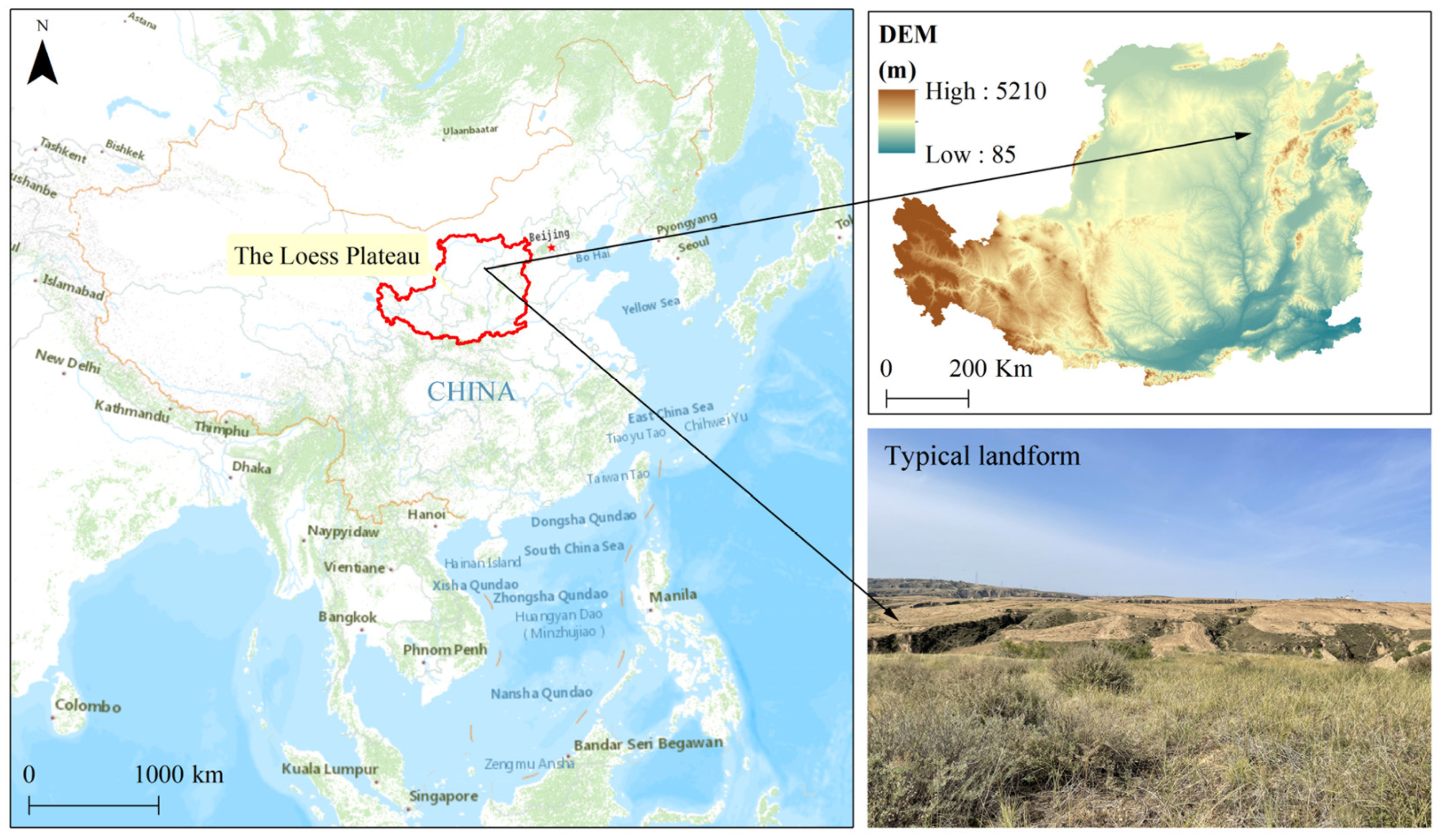
2.1. Study Area

The Loess Plateau is located in the north central region of China. The definition of the extent of the Loess Plateau by Wang et al. through scientific investigation was applied in this study (Figure 1) [34]. It covers an area of 62.46 × 10⁴ km², the whole area of Ningxia Hui Autonomous Region and a part of the area of the Shanxi Province, Shaanxi Province, Henan Province, Gansu Province, Qinghai Province, Inner Mongolia Autonomous Region in China were involved in this study. The Loess Plateau is a unique loess landform area in the world, affected by wind and soil erosion, etc. The terrain is fragmented and ecologically fragile. The soil of Loess Plateau is fine-grained and soft, which is conducive to cultivation. The Loess Plateau is one of China’s energy bases, as large amounts of coal, oil, natural gas, and other energy sources are mined in this area. Within the past two decades, the socio-economic activities in Loess Plateau were increased and the scope of human activities have been expanded, therefore the Loess Plateau has become one of the sources of pressure on local ecological risks.

2.2. Data Source

LULC data (30 m resolution) were obtained from Globeland 30 product (http://www.globallandcover.com/, accessed on 23 January 2022). Nighttime light data were obtained from Resource and Environment Science and Data Center (https://www.resdc.cn/, accessed on 23 January 2022), and Earth Observation Group (https://eogdata.mines.edu/products/vnl/, accessed on 23 January 2022). Population density data were obtained from WordPop (https://www.worldpop.org/, accessed on 23 January 2022). Road and railway data were obtained from the Peking University Geographic Data platform (https://geodata.pku.edu.cn/, accessed on 23 January 2022), Socioeconomic Data and Applications Center (SEDAC) (https://sedac.ciesin.columbia.edu/, accessed on 23 January 2022) and Open StreetMap (OSM) (https://www.openhistoricalmap.org/, accessed on 23 January 2022). Nature reserve data were obtained through the vectorization of the Tianditu data (https://www.tianditu.gov.cn/, accessed on 23 January 2022). Water bodies data were obtained from Open StreetMap (OSM) (https://www.openhistoricalmap.org/, accessed on 23 January 2022). Temperature data covering study area were obtained from China Meteorological Data Service Center (http://data.cma.cn/, accessed on 23 January 2022). DEM data were obtained from Geospatial Data Cloud (https://www.gscloud.cn/, accessed on 23 January 2022). The administrative boundary data were obtained from the Resource and Environment Science and Data Center (https://www.resdc.cn/, accessed on 23 January 2022). All these data were defined a same projected coordinate system: WGS_1984_UTM_zone_48N. The resolution of all data was resampled to 30 m after preprocessing, which is consistent with the LULC data.

2.3. Methods

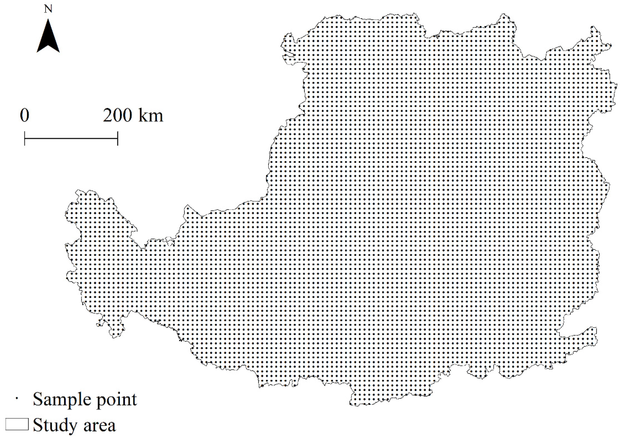
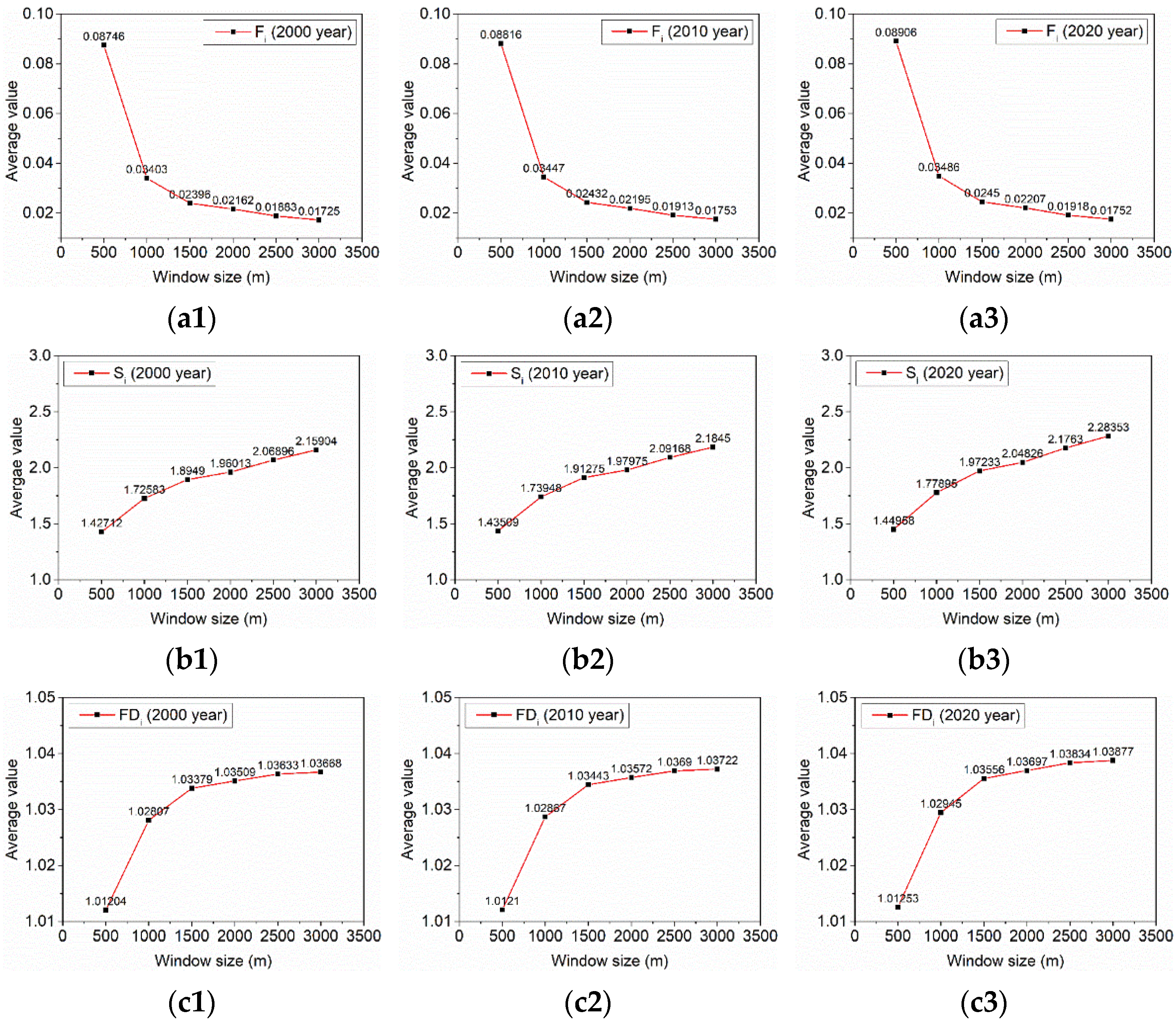
2.3.1. Moving Window

The moving window is a method that can produce a continuous raster data of landscape pattern index based on LULC. Its mechanism is to search the data in the set neighborhood area around its raster by raster, and after calculating by the landscape pattern index equation, the result value of this area is assigned to the central raster until all rasters are assigned, and then the program ends. The shape and distance (window size) of the search range need to be set, and different studies require different parameters of window size.

The moving window method in Fragstats 4.2 software was used to calculate the Landscape Pattern Index. The square with a side length of 500 m, 1000 m, 1500 m, 2000 m, 2500 m, and 3000 m (window shape and it sides) were selected, and the average of the results was calculated by comparing different window sizes to distinguish the optimal computational scales.

2.3.2. Ecological Risk Assessment

An improved landscape ecological risk assessment model that could produce continuous data results was developed based on the landscape ecological risk assessment method of Liu et al. [33]. The LERI was calculated based on the Globeland 30 LULC product.

Before assessing the landscape ecological risk, the Landscape Disturbance Index and the Landscape Vulnerability Index were calculated first.

The Landscape Disturbance Index was calculated by Equation (1):

$$D_i=a{F}_i+b{S}_i+cF{D}_i$$

(1)

In Equation (1), $D_i$ reflects the degree of external disturbance to different landscape ecosystems and is calculated from the Landscape Fragmentation Index ($F_i$), the Landscape Separation Index ($S_i$), and the Landscape Fractal Dimension ($F{D}_i$). Landscape fragmentation has a significant impact on ecosystems and limits ecosystem function [35]. Landscape fragmentation is expressed as the Landscape Fragmentation Index ($F_i$) in this study: $F_i$ is the degree of spatial fragmentation of the landscape, which can reflect the influence of natural or human disturbance on the landscape, and the larger its value, the less stable the landscape is and the greater the degree of disturbance. $S_i$ is the degree of separation of different patches in the landscape and is one of the important indicators to describe the structure of the landscape [36]; its larger value indicates that the more dispersed and the more complex the landscape distribution is. $F{D}_i$ is an indicator used to determine the influence of patch shape on internal ecological processes in the patch, and the larger the value, the more complex the patch shape; at the same time, $F{D}_i$ also represents the roughness of the surface landscape to a certain extent [37]. $a$, $b$, and $c$ are weights, and $a+b+c=1$. Their weight value was determined by referring to the existing literature [33], and a, b, and c were assigned values of 0.5, 0.3, 0.2, respectively. $F_i$, $S_i$, and $F{D}_i$ were calculated according to Equations (2)–(4).

$$F_i=\frac{n_i}{A_i}$$

(2)

$$S_i=\frac{A}{2A_i}\sqrt{\frac{n_i}{A}}$$

(3)

$$F{D}_i=\frac{2\ln \left(\frac{P_i}{4}\right)}{\ln A_i}$$

(4)

In Equations (2)–(4), $n_i$ represents the number of patches of the $i$-th landscape. $A_i$ represents the area of the $i$-th landscape. $A$ is the total area of all landscapes, whose unit is km². $P_i$ is the perimeter of the $i$-th landscape, whose unit is km.

The Landscape Vulnerability Index was obtained by the expert scoring method. $V_i$ reflects the sensitivity of different landscape ecosystems to external disturbances; the larger the $V_i$ value, the more unstable the ecosystem is and the more vulnerable it is to damage [32,33]. Combined with the characteristics of the study area, the 6 types of landscape were assigned values: cultivated land value was 4, forestland was value 2, grassland was value 3, water bodies was value 5, construction land value was 1, and unused land value was 6. Furthermore, the assigned data were normalized [18,32].

The LERI was constructed based on the Landscape Disturbance Index and Landscape Vulnerability Index, and the LERI was used to describe the degree of ecological loss [33]. The higher the value, the higher the ecological risk. The traditional LERI calculation method was based on the calculation of the landscape pattern index ($F_i$, $S_i$, and $F{D}_i$) of each landscape type in each cell grid, and then, the $D_i$ in each cell grid was calculated, and the result resolution was consistent with the cell grid (mostly higher than 10 km result resolution in the Loess Plateau). The equation is:

$$ER{I}_k=\sum _{i=1}^n\frac{A_{ki}}{A_i}\left(D_i{V}_i\right)$$

(5)

where $ER{I}_k$ is the ecological risk index of evaluation unit $k$; $n$ is the number of landscape types; $A_{ki}$ is the area of landscape type $i$ in landscape ecological risk evaluation unit $k$, km²; and $A_i$ is the area of landscape ecological risk evaluation unit $k$, km².

Equation (5) can produce discrete data; the factor that limits its resolution is the calculation of $D_i$, that is, each landscape pattern index is discrete, and each cell grid has only one unique value, while the calculation method that can produce continuous data was developed in this study. The moving window method was used to replace the cell grid method to calculate the overall landscape pattern index ($F_i$, $S_i$, and $F{D}_i$) to obtain a continuous type of $D_i$ data. Therefore, the traditional LERI method in Equation (5) can be simplified. Its mechanism is that, when the ecological risk evaluation unit is infinitely small, i.e., the size of $k$ is equal to the spatial resolution of continuous-type data, at which time there exists and only exists one landscape type inside $k,$ $\frac{A_{ki}}{A_i}$ in Equation (5) is a constant equal to 1. Since the calculation of each landscape pattern index using the moving window method was based on the landscape scale, each landscape type was integrated with the calculation of the landscape pattern index ($F_i$, $S_i$, and $F{D}_i$). So, $\sum _{i=1}^n( )$ in Equation (5) was duplicated. Therefore, the model equation for calculating the ecological risk of a landscape with continuous data is:

$$ER{I}_j=D_{mw,j}·V_j$$

(6)

In Equation (6), $ER{I}_j$ is the Landscape Ecological Risk Index based each raster; $mw$ represents the moving window method; and $j$ represents each raster.

In this study, the new LERI calculation model (Equation (6)) was used to calculate LERI in the Loess Plateau. Since the new model is based on the improvement of traditional methods, the results are similar in the macroscopic view, but the resolution (30 m result resolution in this study) and calculation efficiency of the results can be greatly improved. Furthermore, since the moving window method considers the influence of other raster in the neighborhood (in the window) of the central raster, it is more scientific than traditional methods.

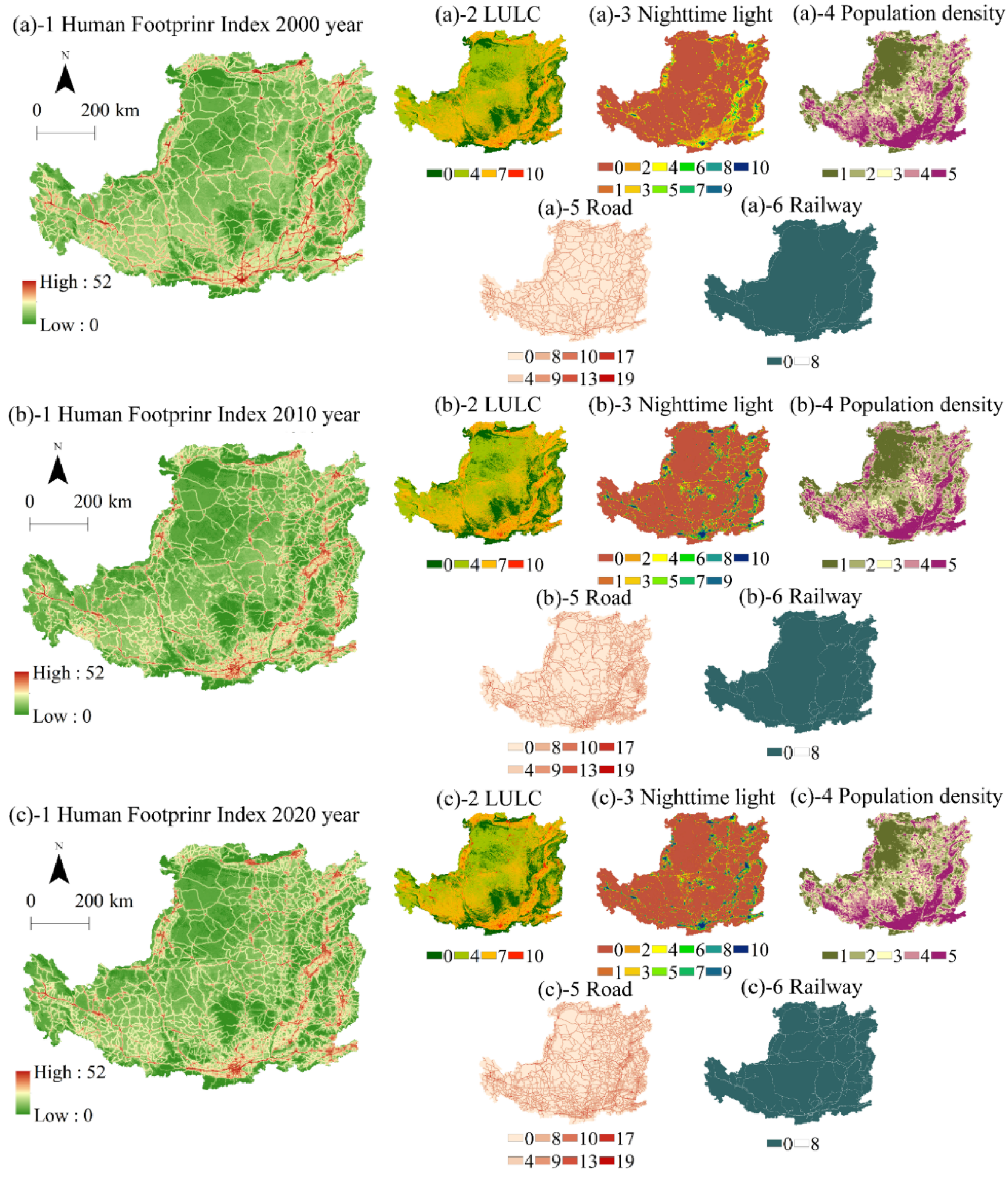
2.3.3. Human Footprint Index

The methodology of Duan and Luo on the human footprint of the Tibetan Plateau was consulted [38]. LUCC, nighttime light, population density, main road, and railway data were selected to contribute to the Human Footprint Index (

Table 1. Human footprint index factors.

Factors	Selection Basis	The Range of Values after Assignment
LUCC	Reflects the degree of human influence on different land types.	0, 4, 7, 10
Nighttime light	Reflects the spatial distribution of the population and towns, as well as economic activities, electricity consumption and carbon emissions.	0–10
Population density	Reflects the number of people per square kilometer.	0–10
Main road	Reflecting the human arrival area, evaluates the scope of impact on the surroundings.	4, 8, 10
Railway	Reflecting the human arrival area, evaluates the scope of impact on the surroundings.	8

). Since the LERI was also calculated based on LULC data, this component was not involved in the analysis of the ecological impact of the Human Footprint Index and its factors on the LERI. So, the LULC data, as an important part of the integrated Human Footprint Index, was used only in the analysis of the spatial and temporal variation of the human footprint and its characteristics in the Loess Plateau.

(1)

Land use and land cover

The Globeland30 product data were used to calculate a part of the Human Footprint Index. Different LULC types differ in population size, human activity carrying capacity, and type of human activity. In this study, construction, arable land, and grassland were assigned 10, 7, and 4 points, respectively, while the rest of the land types were 0 points [38].

(2)

Nighttime light

Nighttime light data were a comprehensive reflection of human activities, such as the extent of population distribution and density, intensity of economic activity, electricity consumption et al. [39,40,41]. The Defense Meteorological Satellite Program-Operational Linescan System (DMSP-OLS) and the Visible Infrared Imaging Radiometer Suite-Day–Night Band (VIIRS-DNB) nighttime light data were used in this study. The methods of Cao et al. were referenced to integrate two different type of nighttime light data [42]. A DN value of 0 area was assigned to 0 points; for a DN value greater than 0 area, the 2020 nighttime light data used the quantile method from small to large in turn into 10 levels, with the corresponding value being assigned to 1–10 points. The data of 2000 and 2010 nighttime light were assigned in accordance with the 2020 level.

(3)

Population density

Population density data are an inaccessible data to characterize the human footprint. Population density not only reflects the area reached by humans, but also the intensity of human activity in the area. Population density data were assigned a score of 1–10, and the assignment formula was determined based on the maximum value of population density per square kilometer:

$$PO{P}_{score}=c\times \log \left(PO{P}_{density}+1\right) \mathrm{where} c=\frac{10}{\log (\max PO{P}_{density}+1)}$$

(7)

In Equation (7), $PO{P}_{score}$ represents the population density score; $PO{P}_{density}$ represents the population density data; $c$ is a constant; and $\max PO{P}_{density}$ represents the maximum value of population density per square kilometer.

(4)

Road

Roads are one of the basic conditions for humans to be able to reach a certain area. The roads in the Loess Plateau can be divided into two categories: the expressway and other roads, including national roads, provincial roads, and county roads. Based on the study by Duan and Luo [38], the assignment of roads was improved in this study to suit the Loess Plateau characteristics. Considering that the Loess Plateau expressway has better closure (higher than other roads and lower than railroads), it was assigned 9 points within 500 m on both sides and 0 points in other ranges. The area within 500 m of the other roads was assigned 10 points; the area within 500–1000 m was assigned 8 points; the area within 1500–2500 m was assigned 4 points; and the other areas were assigned 0 points.

(5)

Railway

Although the railroad has a large capacity compared to the highway, because the railway has a certain closed nature, therefore, the area within 500 m on both sides of the railway was assigned a value of 8 points, while other areas were assigned a value of 0 points [38].

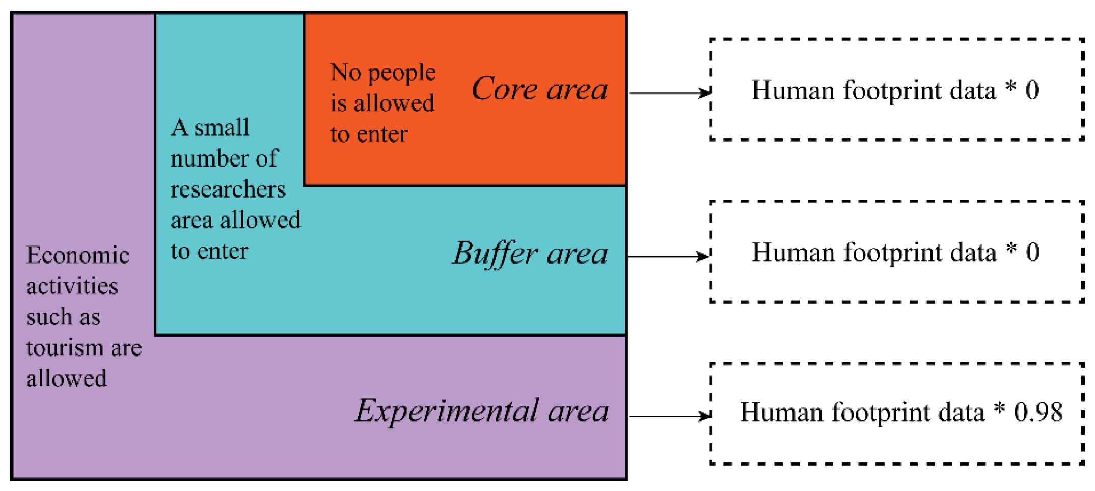
2.3.4. Modification of Human Footprint Data

(1)

Water bodies

Water bodies are areas that are not directly accessible to humans and have little interannual spatial variation in their location. Therefore, the 2020 waterbody extent data were used to make corrections to the human footprint data. The method is to set the raster value to 0 for the areas where human footprint data overlap with water body extent data.

(2)

Nature Reserves

Data on the extent of national nature reserves in China from 2000 to 2020 were used to correct the human footprint data.

The calculation method for the different components of the national nature reserve data used to correct the human footprint data was determined (Figure 2). The human footprint of the core area was corrected to 0 because no people are allowed to enter the core area. Since almost no one is allowed in the buffer zone and the scientific research allowed does not have a negative impact on the local area, the buffer zone and the experimental zone are considered the same according to the latest Chinese policy on the management of national nature reserves. The corrected numerical of experimental area were selected based on the research of Duan and Luo [38] and it was adjusted to adapt the actual in the Loess Plateau.

2.3.5. Climate Change Factors Selection

The potential to drive landscape patterns and ecological risks to the landscape as temperature tends to influence human farming practices, the distribution of forests, and the distribution of settlements. The influence of temperature factor on landscape ecological risk was calculated separately in two ways:

(1)

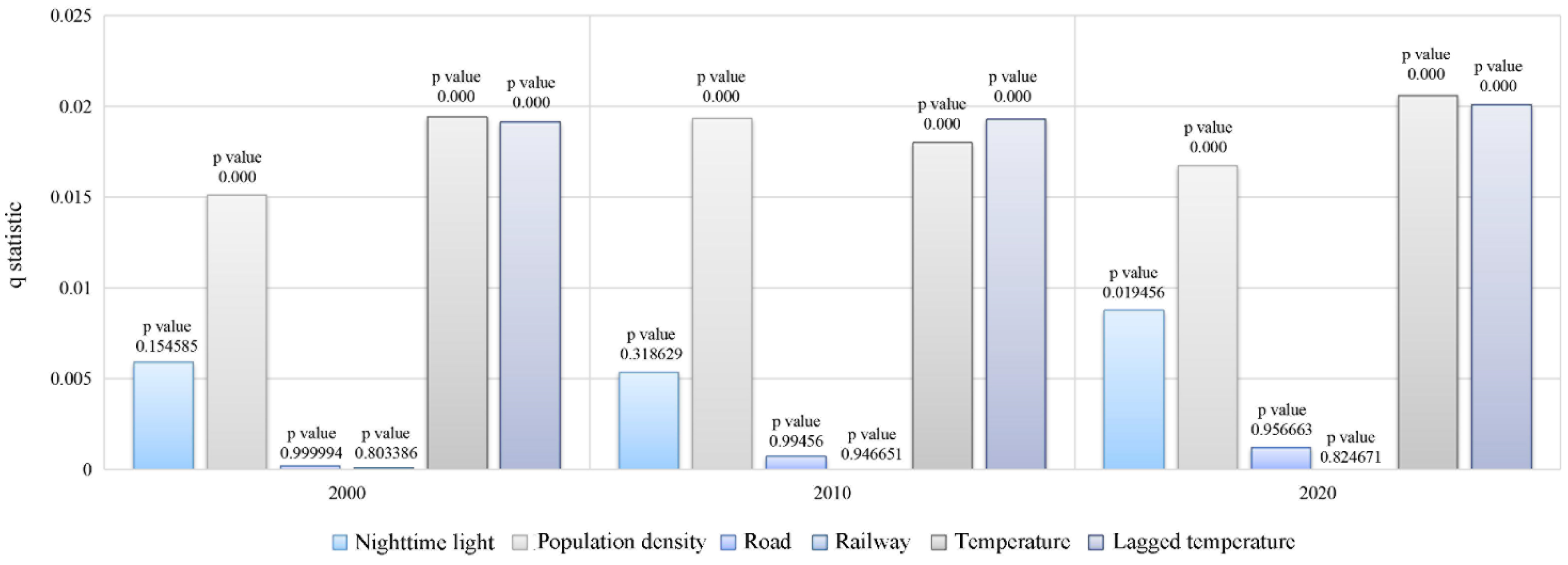
The annual average temperature statistics of the Loess Plateau sub-counties for the years 2000, 2010, and 2020 year were selected to detect the driving forces of spatial evolution of landscape ecological risk in the Loess Plateau.

(2)

Fourcade et al. believe that the response of communities and other ecosystems to climate change is evidently lagging, forming a “climate debt” [43]. Anderegg et al. pointed out that within 1–4 years after encountering extreme weather events, such as drought, the ecosystems, especially forests ecosystem, will be severely affected [44]. Therefore, the average temperature data of the study period and the previous two years were used to calculate the multi-year average temperature (i.e., average lagged temperature) to adapt to the impact of the climate debt.

2.3.6. Geographical Detector Model

The geographical detector (Geodetector) model invented by Wang and Xu in 2017 [45] was used in order to solve the problem of detecting spatial differentiation and driving force. The Geodetector model has 4 sub-modules: factor detector, interaction detector, ecological detector, and risk detector.

(1)

Factor Detector

$$q=1-\frac{{\sum }_{h=1}^L{N}_h{\sigma }_h^2}{N{\sigma }^2}=1-\frac{SSW}{SST} \mathrm{Which} SSW={\sum }_{h=1}^L{N}_h{\sigma }_h^2, SST=N{\sigma }^2$$

(8)

In Equation (8), $q$ is the value of the level at which factor $X$ explains property $Y$. $h=1,\dots ,$ $L$ is variable $Y$ or factor $X$’s strata; $N_h$ and $N$ are the number of cells in strata $h$ and in the entire area, respectively. ${\sigma }_h^2$ and ${\sigma }^2$ are the squares of the $Y$ values of strata $h$ and of the entire region, respectively. $SSW$ and $SST$ are the within sum of squares and the total sum of squares, respectively.

(2)

Interaction Detector

The interaction detector was used to identify the interaction between different risk factors $Xs$, that is, assess whether factors $X1$ and $X2$ work together to increase or decrease the explanatory power of dependent variable $Y$, or whether the effects of these factors on $Y$ are independent of each other. The evaluation method is to first calculate the $q$ value of the two factors $X1$ and $X2$ to $Y$: $q\left(X1\right)$and $q\left(X2\right))$; calculate the value of $q$ when they interact (layer overlay): $q\left(X1\cap X2\right))$; and compare $q\left(X1\right)$, $q\left(X2\right)$, and $q\left(X1\cap X2\right)$. The relationship between the two factors are divided as shown in

Table 2. Type of the interaction detector results.

Judgments Based	Interaction
q(X1 ∩ X2) < Min(q(X1),q(X2))	Weakened, nonlinear
Min(q(X1),q(X2)) < q(X1 ∩ X2) < Max(q(X1),q(X2))	Weakened, nonlinear, single factor
q(X1 ∩ X2) > Max(q(X1),q(X2))	Enhanced, double factor
q(X1 ∩ X2) = q(X1) + q(X2))	Independence
q(X1 ∩ X2) > q(X1) + q(X2))	Enhanced, nonlinear

.

(3)

Ecological Detector

Ecological detectors were used to compare the differences in the relative importance of the explanatory power of different factors. In the ecological detector, significant differences in the effects of the two factors $X1$ and $X2$ on the spatial distribution of attribute $Y$ were compared, as measured by the $F$-statistic.

$$F=\frac{N_{X1}\left(N_{x2}-1\right)SS{W}_{X1}}{N_{X2}\left(N_{x1}-1\right)SS{W}_{X2}} \mathrm{Which} SW{W}_{X1}={\sum }_{h=1}^{L1}{N}_h{\sigma }_h^2, SW{W}_{X2}={\sum }_{h=1}^{L2}{N}_h{\sigma }_h^2$$

(9)

In Equation (9), $N_{X1}$ and $N_{X2}$ refer to the number of samples of the two factors $X1$ and $X2$, respectively; $SS{W}_{X1}$ and $SS{W}_{X2}$ refer to the sum of within-layer variance of the strata formed by $X1$ and $X2$, respectively; $L1$ and $L2$ refer to the number of variables $X1$ and $X2$ strata, respectively. The null hypothesis $H_0$ is: $SS{W}_{X1}=SS{W}_{X2}$, if $H_0$ is rejected at the significance level of $\alpha$. This indicates that there is a significant difference in the effect of the two factors $X1$ and $X2$ on the spatial distribution of attribute $Y$.

(4)

Risk Detector

The risk detector was used to highlight which types of variables have significant high or low values for each human footprint factor. In the risk detector, whether the mean values of the attributes were significantly different between the two sub-regions was determined, using the $t$-statistic to test.

$$t_{{\overline{y}}_{h=1}-{\overline{y}}_{h=2}}=\frac{{\overline{Y}}_{h=1}-{\overline{Y}}_{h=2}}{{\left[\frac{Var\left({\overline{Y}}_{h=1}\right)}{n_{h=1}}+\frac{Var\left({\overline{Y}}_{h=2}\right)}{n_{h=2}}\right]}^{\frac{1}{2}}}$$

(10)

In Equation (10), ${\overline{Y}}_h$ denotes the mean of the attributes in subregion $h$. $n_h$ is the number of samples in subregion $h$, and $Var$ denotes variance. The statistic $t$ approximately obeys the $\mathrm{Student}\prime \mathrm{s} \mathrm{t}$ distribution, where the degrees of freedom are calculated as shown in Equation (10).

$$df=\frac{\frac{Var\left({\overline{Y}}_{h=1}\right)}{n_{z=1}}+\frac{Var\left({\overline{Y}}_{h=2}\right)}{n_{h=2}}}{\frac{1}{n_{h-1}-1}{\left[\frac{Var\left({\overline{Y}}_{h=1}\right)}{n_{h=1}}\right]}^2+\frac{1}{n_{h-2}-1}{\left[\frac{Var\left({\overline{Y}}_{h=2}\right)}{n_{h=2}}\right]}^2}$$

(11)

In Equation (11), the null hypothesis is $H_0$: ${\overline{Y}}_{h=1}={\overline{Y}}_{h=2};$ if $H_0$ is rejected at confidence level $\alpha$, it is considered that there is a significant difference in the mean values of the attributes between the two subregions.

Wang et al. pointed out that, when the Geodetector is used, the X and Y factor data often have different recording methods, so the samples need to be selected and discretized [45]. Too few samples reduces the accuracy of the model results, and a large number of samples increases the amount of the calculation. In this study, evenly distributed sample points with an interval of 10 km were selected, a total of 6265 sample points (Figure 3).

3. Results

3.1. Moving Window

The size of the moving window needed to be set according to the different study areas. A window that is of too large a size will cause the resultant layer to be too blurred, and a window that is of too small a size will cause the calculation to grow exponentially.

A set of comparison experiments was used to select the appropriate window size. The average value of the Loess Plateau’s three landscape pattern indices, $F_i$, $S_i$, and $F{D}_i,$ in 2000, 2010 and 2020 were used to compare and observe the changes in the average values of their calculated results under different window sizes (Figure 4).

The experimental results show that, as the window size changes, the average value of the landscape pattern index first shows a drastic change, and after a certain node, it starts to slow down, after which it enters a flatter state and no longer changes drastically with the window size (Figure 4). Selecting the window size of the nodes that enter the smoothed state can ensure that the computation is not too large, while maximizing the stability of the results. As the window size increases, the average value of the $F_i$ index maintains a downward trend (Figure 4a), while the average values of the $S_i$ index and $F{D}_i$ index maintain an upward trend; compared with the $S_i$ index, the average value of the $F{D}_i$ index has a larger change in window size between 500 m and 1000 m (Figure 4b,c). The common feature of each variation of average value of the Loess Plateau landscape pattern index is that they vary considerably between the window size of 500 m and 1000 m, and this variation continues up to 1500 m, after which the variation tends to stabilize. Therefore, the optimal scale (window size) for this study is 1500 m.

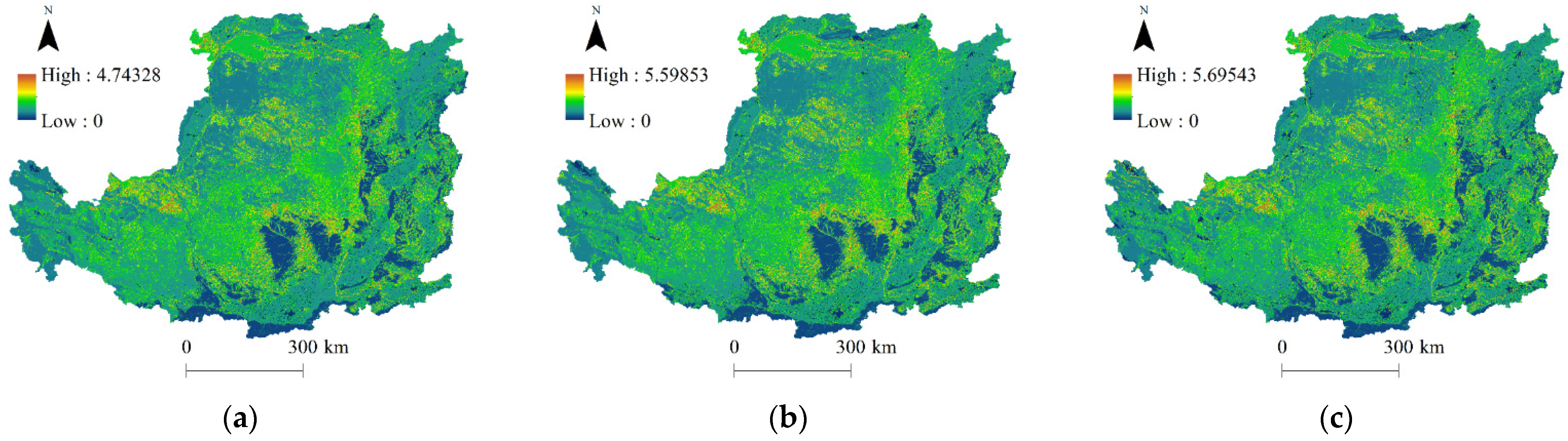
3.2. LERI of Loess Plateau

Based on the moving window method and landscape pattern index, the LERI was calculated using Equation (6).

The high-value areas of LERI are more spatially dispersed compared to the low-value areas (Figure 5). The highest values of LERI in 2000, 2010, and 2020 were 4.74328, 5.59853, and 5.695543, respectively, reflecting that, from 2000 to 2020, areas with more serious landscape ecological risks continued to appear in the Loess Plateau. The high-value area of LERI is mainly located in the central part of the Loess Plateau. The distribution of low-value areas of LERI has the following characteristics: (1) the area with a low value of LERI in the southeast of the Loess Plateau is large, and the area with a low value of LERI is rarely seen in the northwest; (2) although the area with a low value of LERI in the northwest region is small, there are obviously many small and discontinuous low values of LERI areas added (Figure 6a–c).

(3) In urban areas, the LERI value remains at a low level (Figure 6d–f), because urban areas are often in a relatively stable ecological environment. Often in the transitional areas between population clusters and natural areas, there is high ecological instability. Human footprints or the impact of human activities on the ecology also occur more often in these areas. The transitional areas between cities and villages are also more prone to this situation, such as the agro-pastoral transition zone, urban–rural transition zone, and foothills [24,25]. This phenomenon can be seen in Figure 6, where the transitional area between the mountain and the plain in the southern area of Xi’an, distributed along the edge of the mountain, is a strip of a higher value of LERI regions that runs east–west.

In order to compare the changes of LERI data more clearly in 2000, 2010 and 2020 in the same standard, LERI data in ArcGIS10.3 platform were divided into five grades according to the quantile of LERI in 2020. From low to high, they are the lowest, lower, medium, higher and highest, and the area statistics are made (

Table 3. The area of each LERI level.

Area (km2)	Lowest	Lower	Medium	Higher	Highest
2000 year	85,371.6501	167,656.8708	135,642.7890	119,017.3698	113,566.1553
2010 year	93,878.2602	159,297.2541	133,951.2966	119,551.9689	114,575.6772
2020 year	106,367.3118	140,546.9430	132,820.7013	120,801.3426	120,718.5363

).

According to Table 3, the LERI lower level had the highest percentage of area between 2000 to 2020 year, but its area shows a trend of rapid decline. The area of the medium level and higher level maintain a stable trend, and the area of the highest level have a significant increase, especially between 2010 and 2020. The area of the lowest class increased rapidly, but its proportion remained the smallest.

3.3. Human Footprint of Loess Plateau

The Human Footprint Index of Loess Plateau in 2000, 2010, and 2020 was constructed. According to the Integrated Human Footprint Index (Figure 7), the southern and southeastern parts of the Loess Plateau, as well as the marginal areas in the northwest and north, have the highest value Human Footprint Index, and the lowest value areas are mainly located in the periphery of the high-value areas in the southeast, as well as in the northwestern region. From the southeast to the northwest, the Human Footprint Index trends roughly in the order of highest value, lowest value, medium or lower value, lowest value, and highest value.

The LULC and nighttime light factors show a continuous trend of major city area expansion, and this change is particularly evident in the 2000–2010 period for the nighttime light data, which not only reflects the change in city area expansion from 2000–2010, but also shows an increase in spatial aggregation of nighttime light in the southeastern region of the Loess Plateau [Figure 7((a)-2,(b)-2,(c)-2,(a)-3,(b)-3,(c)-3)].

The population density factor reflects that the areas where the population is concentrated are located in the south and southeast of the Loess Plateau, and the population density low value is located in the north and northwest. The area with the population density lowest value with level 1 is located in the northwest of the Loess Plateau, and the area of such areas, from 2000 to 2020, significantly reduced (Figure 7((a)-4,(b)-4,(c)-4)).

Road and railway lengths and densities continued to increase from 2000 to 2020, concentrated in the southeast region [Figure 7((a)-5,(a)-6,(b)-5,(b)-6,(c)-5,(c)-6))].

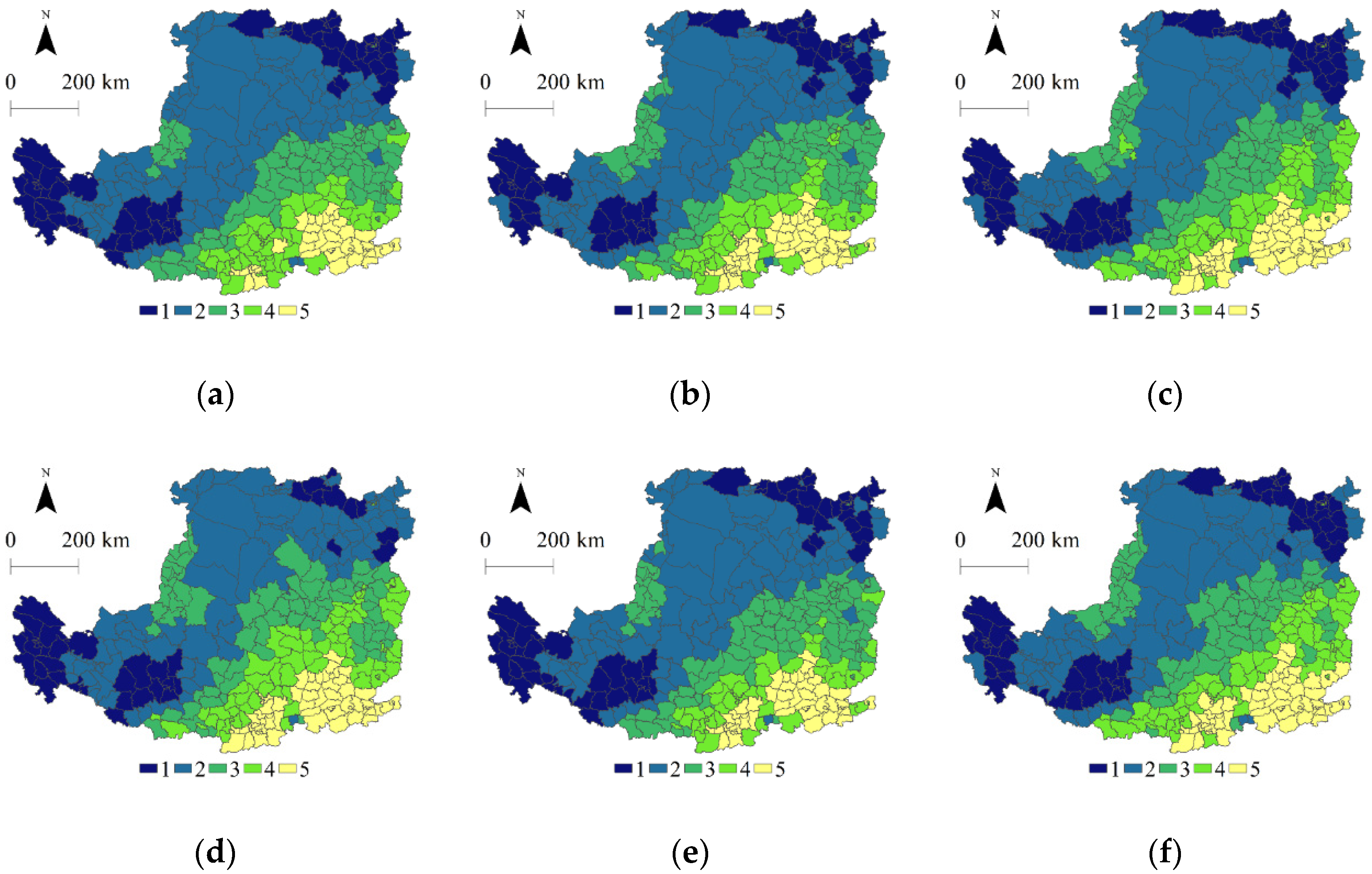
3.4. Climate Factor of Loess Plateau

In this study, the climate factor was expressed by two factors, the average temperature of county scale and the average lagged temperature, which considers the temperature lag effect.

The temperature factor was divided into five classes based on the average temperature quantile in 2020 in order from lowest to highest. Areas below 7.322050 °C are level 1, areas below 9.716185 °C and above 7.322050 °C are level 2, areas below 11.169613 °C and above 9.716185 °C are level 3, areas below 13.296754 °C and above 11.169613 °C are level 4, and areas above 13.296754 are level 5 (Figure 8).

The Loess Plateau region is mainly affected by the warm temperate semi-arid continental monsoon climate, with an annual average temperature of about 4 to 12 °C [46]. Both the average temperature factor and average lagged temperature factor show a decreasing trend from southeast to northwest in spatial distribution, but there are anomalous regions among them. In the high temperature class area in the southeast of the Loess Plateau, there exists a small area of lower classes, which are located in the mountainous areas on the edge of the Loess Plateau, and their low temperatures are more likely to be influenced by topography. In the western low temperature class area of the Loess Plateau, there exist slightly larger areas of relatively higher-level temperature class areas, which are located in the rare areas in the west where population and traffic are more concentrated.

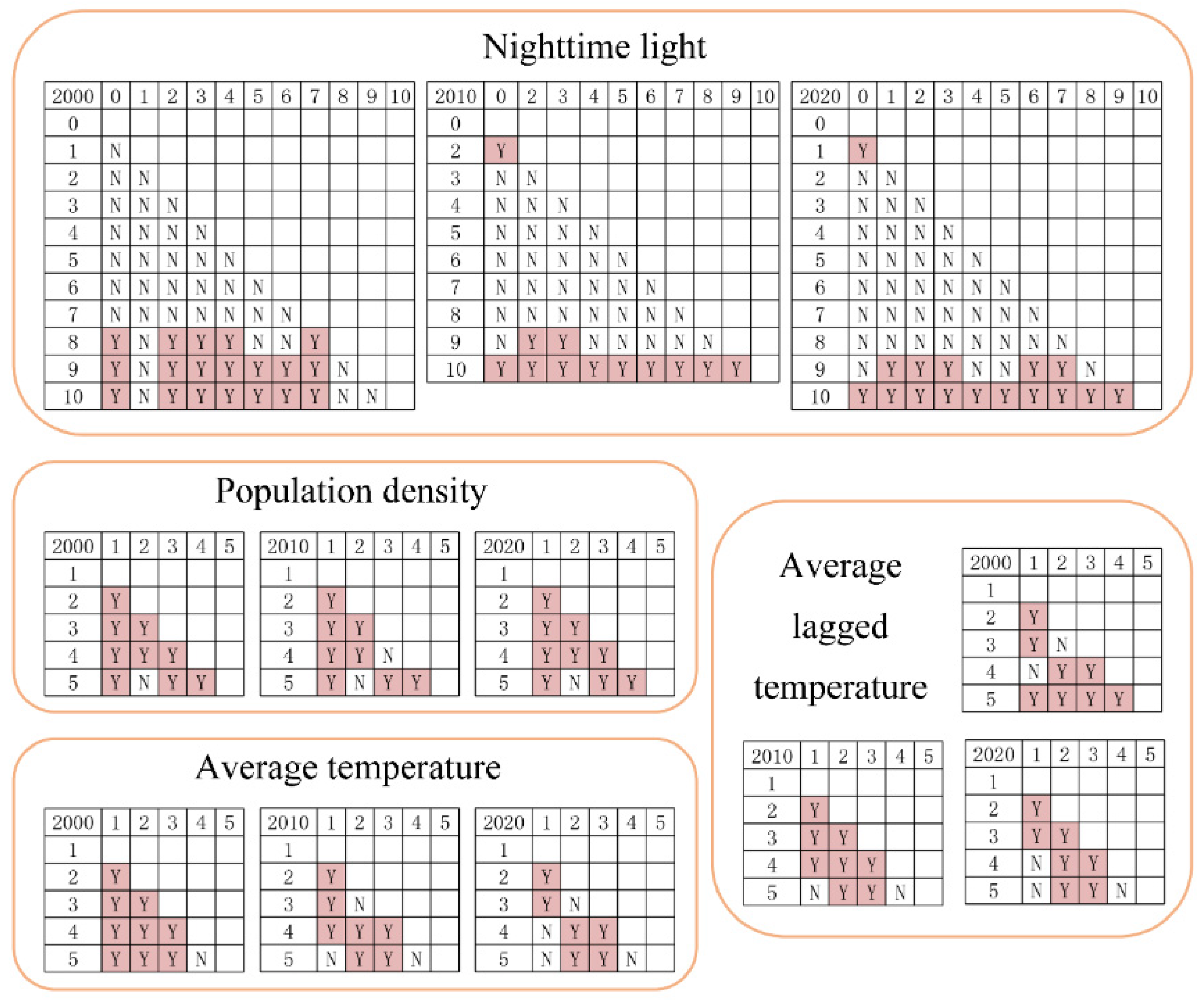
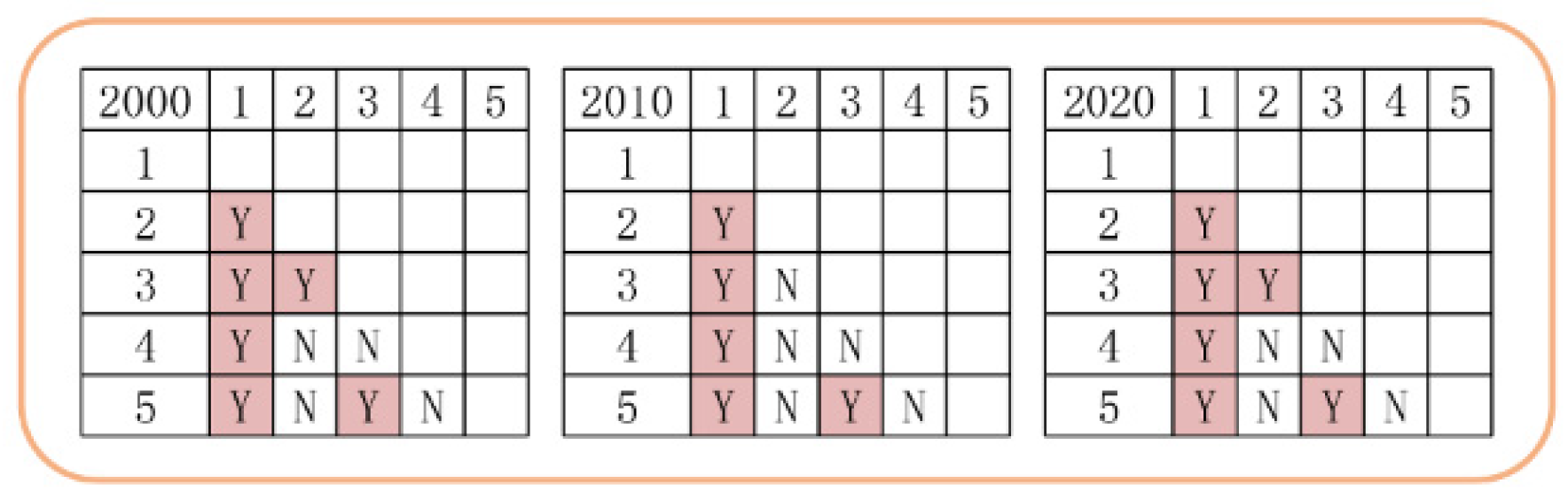
3.5. Driving Factor Explore Result Using the Geographical Detector Model

The geographical detector model (Geodetector) was used to detect driving factors of LERI in the Loess Plateau.

Based on the Human Footprint Index, the detection of ecological risk for the Loess Plateau landscape is divided into two parts: individual detection and overall detection of each factor.

In terms of individual detection of each factor, the factor detector, the interaction detector, the ecological detector, and the risk detector were used to perform three periods of each human footprint factors data for the years 2000, 2010 and 2020.

Because two and more factors are required for the operation of the interaction detector and the ecological detector, in terms of overall detection, the factor detector and the risk detector in the Geodetector were used to perform three periods of the Human Footprint Index for the years 2000, 2010 and 2020.

3.5.1. Geodetector Runs for Each Individual Factor Result

(1)

Factor Detector Result

Factor detectors were used to detect the extent to which the independent variable explained the dependent variable. The dependent variable is LERI, and each human footprint factors and climate factors (except for the LUCC factor) were used as independent variables and were simultaneously calculated by the model (Figure 9).

The $q$ statistic in the factor detector is used to indicate the extent to which the dependent variable is explained by the independent variable. A larger $q$ indicates that the independent variable explains the dependent variable to a greater extent. The $p$ value is used to indicate the degree of significance: the smaller the $p$, the higher the degree of significance.

Except for the road and rail factors in each year, all other factors maintain a low $p$ value, which indicates a high confidence. The reason is that roads and railroads are similar to linear features, and although values were assigned to their surrounding areas, they still occupied a small area relative to the study area, resulting in larger $p$ values.

For the Human Footprint Index, the population density factor explained the LERI to the highest degree, followed by the nighttime light factor. The road factor explains the LERI to a greater extent than the rail factor.

In terms of climate factors, the difference in the degree of LERI explained by the average temperature and average lagged temperature factors is small, with the average temperature factor being slightly higher relative to the average lagged temperature factor in 2000 and 2020, but the average lagged temperature factor being much higher than the average temperature factor in 2010.

(2)

Interaction Detector Result

In 2000, the two-factor interaction result is enhanced-nonlinear, except for $Railway \cap Temperature$ and $Average temperature \cap Average lagged temperature$, where the result is enhanced-double factor. That is, all the factor interactions except these two result in highly strengthening, while the interaction between $Railway \cap Temperature$ and $Average temperature \cap Average lagged temperature$, although also strengthening, is not highly significant.

The interaction detector results for 2010 and 2020 are similar. Except for $Average temperature \cap Average lagged temperature$, where the result is enhanced-double factor, all other factor interactions result in enhanced-nonlinear.

Taken together, when the human footprint factors and climate factors have an impact on the LERI, the simultaneous impact on the LERI between any two factors is greater than the impact on the LERI by individual factors.

(3)

Ecological Detector and Risk Detector Result

The ecological detector was used to detect whether the effects of two independent variables on the spatial distribution of the dependent variable were significantly different. Additionally, the risk detector was used to detect if there was a significant difference in the mean value of an attribute between two sub-areas.

According to the results of the ecological detector, there is no significant difference in the effect of all two factors on the spatial distribution of the dependent variable LERI in 2000, 2010, and 2020 (F test: 0.05), i.e., there were no significant differences in the relative importance of the human footprint factors in terms of their impact on LERI. This also indicates that, although the explanatory power of the road and rail factors on LERI in the factor detector is small compared to other human footprint factors, it does not affect the fact that in practice the road and rail factors have an impact on LERI within a certain range.

According to the risk detector results, in terms of the road factor in 2000, 2010, and 2020, there is no significant difference between the average values of the attributes except in the 0 value region and the 8 value region in 2020. The rail factor in 2000, 2010, and 2020 was not significantly different to the risk detector results. The risk detector results for the other factors are presented in Figure 10. The color-marked Y represents the presence of significant high or low values of the human footprint factor between these types of variables.

3.5.2. Geodetector Runs for the Integrated Human Footprint Index Results

The Integrated Human Footprint Index without the LULC factor was calculated and the extent of its influence on the LERI was explored using the factor detector. The results show that the $q$ statistic in the 2000, 2010, and 2020 was 0.006792, 0.011096, and 0.008495, respectively. In 2000 and 2010, except below the population density factor $q$ statistic, it was higher than the other human footprint factors $q$ statistic. In 2020, it was lower than the population density factor $q$ statistic and essentially the same as the nighttime light factor $q$ statistic. Meanwhile, the stability of the Integrated Human Footprint Index without the LULC factor was reduced and did not show a clear pattern of change.

According to the risk detector results of the Integrated Human Footprint Index without the LULC factor, compared with the area with level 1, the average value of attributes of most level areas is significantly different from it (Figure 11).

4. Discussion

In this section, the study methodology and details of the study results are described and discussed. Furthermore, the innovation and limitation aspects of the study are highlighted.

In the construction of the road factor, national roads, provincial roads, and highways that have a high traffic volume were selected. Lower-level roads were not selected because most of these lower-level roads are located around construction land, which was assigned several times in other factors, and were not considered in the data selection of the road factor in order to avoid repeated assignments and their low importance to the Loess Plateau.

The pattern of climate change requires long-term observation data that include the observation of temperature [47]. For example, in observing climate change patterns on a large regional or global scale, generally, about 30 years of observation data are required [48]. A generalized pattern of temperature change is difficult to obtain from the three-period average temperature and average lagged temperature data, so this data were only analyzed in this study as the driving factors of LERI in the corresponding years, and their trends and patterns are not summarized.

The Human Footprint Index constructed in this study, its factor selection and assignment were determined through references, and a part of them was adjusting the, to be adapted to the actuality of the Loess Plateau. Furthermore, according to the results of the study, the degree of influence of human footprint on LERI showed an unstable trend, and a downward trend from 2010 to 2020. The driving force of LERI became progressively more complex, because the type of activity of each human generation has an impact on the ecosystem at that time, as well as on subsequent ecosystems, ultimately creating an intricate mechanism of influence [49]. However, the selection of each factor of Human Footprint Index was fixed, and with the development of society and the economy, the types of human activities were bound to become more and more diversified, so the dynamic selection of factors that changed over time was considered reasonable, but its theory basis needs to be further explored.

Assigning values to various human footprint factors often ignores the dynamic changes in the weights of different regions and simplifies the complexity of human activities. However, this method is still a suitable method for constructing indexes, such as the human footprint in a large-scale area. A more dynamic method can be envisaged—that is, the dynamic assignment according to the time and space adapted to different sub-regions of the study area—and requires the accumulation of a large amount of survey results. The construction of large-scale datasets is time consuming and labor intensive, but with the accumulation of research data, the feasibility of this method will be greatly improved in the future.

In this study, the moving window method was used in the LERI model improvement research for the first time, and a LERI calculation model was developed, which is more simplified than the traditional grid method model, and greatly improves the efficiency of constructing large-scale regional LERI datasets. Once suitable research is determined, the size of the moving window of the region and the number of subsequent calculations will be greatly reduced. At the same time, it measures the direct or indirect impact of human activities on LERI, providing a scientific decision-making basis for the ecological risk management of the Loess Plateau.

5. Conclusions

The LERI construction based on the moving window method achieved the expected effect, and the LERI of the Loess Plateau was constructed at a higher resolution scale. The low-value areas of the LERI spatial distribution of the Loess Plateau are concentrated in the southeast, and higher LERI extreme values continued to appear in 2000, 2010, and 2020. The influence of the Human Footprint Index on LERI under the integrated effect is higher than part of the individual human footprint factor. The influence of the average temperature on LERI was higher than the average lagged temperature in 2000 and 2020, but slightly lower than the average lagged temperature in 2010, and the two temperature factors have little difference in the effect of LERI. The extent of the impact on LERI is enhanced by the combined effect of two individual human footprint factors. Under the single factor effect, the strongest effect on LERI is the population density factor, followed by the nighttime light factor. In terms of climatic factors, both mean and average lagged temperatures had a significant effect on LERI. This effect is even higher than the population density factor of the Human Footprint Index. Although the degree of explanation (impact) of the LERI on the interaction of the two human footprint factors was enhanced compared with these factors acting separately, the degree of explanation of the LERI was not the highest when all single factors acted simultaneously.

According to the result, these research questions can be answered. (1) Based on the new LERI calculation model result, it is feasible to improve both resolution and computational efficiency at the same time. (2) Temperatures do have a significant effect on landscape ecological risk. (3) Although the Loess Plateau has become better overall in terms of landscape ecological risk between 2000 and 2020, the phenomenon of increasing extreme values of risk and expansion of the highest risk level area should become the focus of ecological risk control in the Loess Plateau in the future. (4) The human footprint factor that has the greatest direct impact on the Loess Plateau is population density.

Differences exist in this study, and the main driving factors of LERI are different in different regions, as the Loess Plateau and other areas of the world have different ecological conditions. Additionally, there are also differences in the sub-regions within the study area, such as in areas of rapid population growth and dense road areas. In the future, more of these details will be uncovered as the data accumulate. Additionally, the model proposed in this study will be applied in more regions, including regions with different ecological or development conditions, and thus the model will be further optimized, not only in terms of resolution of results, computational efficiency, etc., but also in terms of scientific validity.

References

1. Peng, J.; Wang, Y.; Wu, J.; Zhang, Y. Evaluation for regional ecosystem health: Methodology and research progress. Acta Ecol. Sin. 2007, 27, 4877–4885. [Google Scholar] [CrossRef]
2. Wu, J. Landscape sustainability science: Ecosystem services and human well-being in changing landscapes. Landsc. Ecol. 2013, 28, 999–1023. [Google Scholar] [CrossRef]
3. Summer, J.K.; Smith, L.M.; Case, J.L.; Linthurst, R.A. A Review of the Elements of Human Well-Being with an Emphasis on the Contribution of Ecosystem Services. Ambio 2012, 41, 327–340. [Google Scholar] [CrossRef] [PubMed] [Green Version]
4. Assesment, M.E. Ecosystems and human well-being: Synthesis. Phys. Teach. 2005, 34, 534. [Google Scholar]
5. Wei, J.; Xiao, D.; Xie, F. Evaluation and Regulation Principles for the Effects of Human Activities on Ecology and Environment. Prog. Geogr. 2006, 25, 36–45. [Google Scholar]
6. Zheng, H.; Ouyang, Z.; Zhao, T.; Li, Z.; Xu, W. The impact of human activities on ecosystem services. J. Nat. Resour. 2003, 18, 118–126. [Google Scholar]
7. Chapman, D.S.; Gunn, I.D.M.; Pringle, H.E.K.; Siriwardena, G.M.; Taylor, P.; Thackeray, S.J.; Willby, N.J.; Carvalho, L. Invasion of freshwater ecosystems is promoted by network connectivity to hotspots of human activity. Global Ecol. Biogeogr. 2020, 29, 645–655. [Google Scholar] [CrossRef] [Green Version]
8. Vitousek, P.M.; Mooney, H.A.; Lubchenco, J.; Melillo, J.M. Human Domination of Earth’s Ecosystems. Science 1997, 277, 494–499. [Google Scholar] [CrossRef] [Green Version]
9. Yu, T.; Bao, A.; Xu, W.; Guo, H.; Jiang, L.; Zheng, G.; Yuan, Y.; Nzabarinda, V. Exploring Variability in Landscape Ecological Risk and Quantifying Its Driving Factors in the Amu Darya Delta. Int. J. Environ. Res. Public Health 2019, 17, 79. [Google Scholar] [CrossRef] [Green Version]
10. Peng, J.; Dang, W.; Liu, Y.; Zong, M.; Hu, X. Review on landscape ecological risk assessment. Acta Geogr. Sin. 2015, 70, 664–677. [Google Scholar]
11. Liu, H.; Liu, L.; Ding, S. The impact of human activities on ecosystem services flow. Acta Ecol. Sin. 2017, 37, 3232–3242. [Google Scholar]
12. Cao, Q.; Zhang, X.; Ma, H.; Wu, J. Review of landscape ecological risk and an assessment framework based on ecological services: ESRISK. Acta Geogr. Sin. 2018, 73, 843–855. [Google Scholar]
13. Peng, J.; Zong, M.; Hu, Y.; Liu, Y.; Wu, J. Assessing Landscape Ecological Risk in a Mining City: A Case Study in Liaoyuan City, China. Sustainability 2015, 7, 8312–8334. [Google Scholar] [CrossRef] [Green Version]
14. Xie, H.; Wen, J.; Chen, Q.; Wu, Q. Evaluating the landscape ecological risk based on GIS: A case-study in the Poyang Lake region of China. Land Degrad. Dev. 2021, 32, 2762–2774. [Google Scholar] [CrossRef]
15. Fu, W.; Lv, Y.; Fu, B.; Hu, W. Landscape Ecological Risk Assessment Under the Influence of Typical Human Activities in Loess plateau, Northern Shaanxi. J. Ecol. Rural Environ. 2019, 35, 290–299. [Google Scholar]
16. Wang, F.; Ye, C.; Hua, J.; Li, X. Coupling relationship between urban spatial expansion and landscape ecological risk in Nanchang City. Acta Ecol. Sin. 2019, 39, 1248–1262. [Google Scholar]
17. Liao, J.; Jia, Y.; Tang, L.; Huang, Q.; Wang, Y.; Huang, N.; Hua, L. Assessment of urbanization-induced ecological risks in an area with significant ecosystem services based on land use/cover change scenarios. Int. Sust. Dev. World 2017, 25, 448–457. [Google Scholar] [CrossRef]
18. Lou, N.; Wang, Z.; He, S. Assessment on Ecological Risk of Aha Lake National Wetland Park Based on Landscape Pattern. Res. Soil Water Conserv. 2020, 27, 233–239. [Google Scholar]
19. Zhang, W.; Chang, W.J.; Zhu, Z.C.; Hui, Z. Landscape ecological risk assessment of Chinese coastal cities based on land use change. Appl. Geogr. 2020, 117, 102174. [Google Scholar] [CrossRef]
20. Zhao, G.; Liu, J.; Kuang, W.; Ouyang, Z.; Xie, Z. Disturbance impacts of land use change on biodiversity conservation priority areas across China: 1990–2010. Acta Geogr. Sin. 2015, 25, 515–529. [Google Scholar] [CrossRef] [Green Version]
21. Liu, J.; Wang, M.; Yang, L. Assessing Landscape Ecological Risk Induced by Land-Use/Cover Change in a County in China: A GIS- and Landscape-Metric-Based Approach. Sustainability 2020, 12, 9037. [Google Scholar] [CrossRef]
22. Xu, W.; Wang, J.; Zhang, M.; Li, S. Construction of landscape ecological network based on landscape ecological risk assessment in a large-scale opencast coal mine area. J. Cleaner Prod. 2020, 286, 125523. [Google Scholar] [CrossRef]
23. Mo, W.; Wang, Y.; Zhang, Y.; Zhuang, D. Impacts of road network expansion on landscape ecological risk in a megacity, China: A case study of Beijing. Sci. Total Environ. 2017, 574, 1000–1011. [Google Scholar] [CrossRef] [PubMed] [Green Version]
24. Jing, Y.; Zhang, S.; Li, Y. Ecological analysis of rural-urban ecotone based on landscape structure. Chin. J. Ecol. 2008, 27, 229–234. [Google Scholar]
25. Yan, J.; Li, G.; Qi, G.; Qiao, H.; Nie, Z.; Huang, C.; Kang, Y.; Sun, D.; Zhang, M.; Kang, X.; et al. Landscape ecological risk assessment of farming-pastoral ecotone in China based on terrain gradients. Hum. Ecol. Risk Assess. 2021, 27, 2124–2141. [Google Scholar] [CrossRef]
26. Kienast, F.; Wildi, O.; Brzeziecki, B. Potential impacts of climate change on species richness in mountain forests—An ecological risk assessment. Biol. Conserv. 1998, 83, 291–305. [Google Scholar] [CrossRef]
27. Landis, W.G.; Durda, J.L.; Brooks, M.L.; Chapman, P.M.; Menzie, C.A.; Stahl, R.G.; Stauber, J.L. Ecological risk assessment in the context of global climate change. Environ. Toxicol. Chem. 2012, 32, 79–92. [Google Scholar] [CrossRef]
28. Shi, H.; Chen, J. Characteristics of climate change and its relationship with land use/cover change in Yunnan Province, China. Int. J. Climatol. 2018, 38, 2520–2537. [Google Scholar] [CrossRef]
29. Wu, L.; Hou, X.; Di, X. Assessment of regional ecological risk in coastal zone of Shandong Province. Chin. J. Ecol. 2014, 33, 214–220. [Google Scholar]
30. Shi, H.; Yang, Z.; Han, F.; Shi, T.; Li, D. Assessing Landscape ECOLOGICAL Risk for a World Natural Heritage Site: A Case Study of Bayanbulak in China. Pol. J. Environ. Stud. 2015, 24, 269–283. [Google Scholar] [CrossRef]
31. Zhou, S.; Chang, J.; Hu, T.; Luo, P.; Zhou, H. Spatiotemporal Variations of Land Use and Landscape Ecological Risk in a Resource-Based City, from Rapid Development to Recession. Pol. J. Environ. Stud. 2020, 29, 475–490. [Google Scholar] [CrossRef]
32. Liu, M.; Wang, Y.; Pei, H. Landscape Ecological Risk Assessment in Bashang Area of Hebei Province Based on Land Use Change. Bull. Soil Water Conserv. 2020, 40, 303–311. [Google Scholar]
33. Liu, X.; Li, X.; Jiang, D. Landscape pattern identification and ecological risk assessment using land-use change in the Yellow River Basin. Trans. Chin. Soc. Agric. Eng. 2021, 37, 265–274. [Google Scholar]
34. Wang, Z. Boundary data of Loess Plateau region. In Global Change Research Data Publishing & Repository; Institute of Geographic Sciences and Natural Resources Research: Beijing, China, 2015. [Google Scholar] [CrossRef]
35. Shao, D.; Wu, D. Analysis on the Effect of Landscape Fragmentation on Ecosystem Service Value: A Case Study of Suzhou. Resour. Environ. Yangtze Basin 2020, 29, 2346–2449. [Google Scholar]
36. Chen, L.; Fu, B. Anlalysis of Impact of Human Activity on Landscape Structure in Yellow River Delta—A Case Study of Dongying Region. Acta Ecol. Sin. 1996, 16, 337–344. [Google Scholar]
37. Lifton, N.A.; Chase, C.G. Tectonic, climatic and lithologic influences on landscape fractal dimension and hypsometry: Implications for landscape evolution in the San Gabriel Mountains, California. Geomorphology 1992, 5, 77–114. [Google Scholar] [CrossRef]
38. Duan, Q.; Luo, L. A dataset of human footprint over the Qinghai-Tibet Plateau during 1990–2015. China Sci. Data 2020, 5, 303–312. [Google Scholar] [CrossRef]
39. Tan, M.; Li, X.; Li, S.; Xin, L.; Wang, X.; Li, Q.; Li, W.; Li, Y.; Xiang, W. Modeling population density based on nighttime light images and land use data in China. Appl. Geogr. 2018, 90, 239–247. [Google Scholar] [CrossRef]
40. Li, X.; Xu, H.; Chen, X.; Li, C. Potential of NPP-VIIRS Nighttime Light Imagery for Modeling the Regional Economy of China. Remote Sens. 2013, 5, 3057–3081. [Google Scholar] [CrossRef] [Green Version]
41. Shi, K.; Yu, B.; Huang, Y.; Hu, Y.; Yin, B.; Chen, Z.; Chen, L.; Wu, J. Evaluating the Ability of NPP-VIIRS Nighttime Light Data to Estimate the Gross Domestic Product and the Electric Power Consumption of China at Multiple Scales: A Comparison with DMSP-OLS Data. Remote Sens. 2014, 6, 1705–1724. [Google Scholar] [CrossRef] [Green Version]
42. Cao, Z.; Wu, Z.; Kuang, Y.; Huang, N. Correction of DMSP/OLS Night-time Light Images and Its Application in China. J. Geo-Inf. Sci. 2015, 17, 1092–1102. [Google Scholar]
43. Fourcade, Y.; WallisDeVries, M.F.; Kuussaari, M.; Swaay, C.A.M.; Heliölä, J.; Öckinger, E. Habitat amount and distribution modify community dynamics under climate change. Ecol. Lett. 2021, 24, 950–957. [Google Scholar] [CrossRef] [PubMed]
44. Anderegg, W.R.L.; Schwalm, C.; Biondi, F.; Camarero, J.J.; Koch, G.; Litvak, M.; Ogle, K.; Shaw, J.D.; Shevliakova, E.; Williams, A.P.; et al. Pervasive drought legacies in forest ecosystems and their implications for carbon cycle models. Science 2015, 349, 520–532. [Google Scholar] [CrossRef] [PubMed] [Green Version]
45. Wang, J.; Xu, C. Geodetector: Principle and prospective. Acta Geogr. Sin. 2017, 72, 116–134. [Google Scholar]
46. Ren, J.; Peng, S.; Cao, Y.; Huo, X.; Chen, Y. Spatiotemporal Distribution Characteristics of Climate Change in the Loess Plateau from 1901 to 2014. J. Nat. Resour. 2018, 33, 621–633. [Google Scholar]
47. Zhang, R. Climate Observing System and Related Crucial Issues. J. Appl. Meteor. Sci. 2006, 17, 705–710. [Google Scholar]
48. Henson, S.A.; Beaulieu, C.; Lampitt, R. Observing climate change trends in ocean biogeochemistry: When and where. Glob. Chang. Biol. 2016, 22, 1561–1571. [Google Scholar] [CrossRef] [PubMed] [Green Version]
49. Wang, X.; Zhang, Q.; Liu, X.; Wen, W. Concept and Standard of Ecological Compensation, and Roles of Human Activities to Ecological System. China Popu. Res. Envi. 2010, 20, 41–50. [Google Scholar]
Figure 1. Study area.
Land 11 00217 g001
Figure 2. Description of the valuation method of nature reserves. (* in the figure represent ×.)
Land 11 00217 g002
Figure 3. Sample points of the Loess Plateau.
Land 11 00217 g003
Figure 4. (a1a3) are F i index average value change with different moving window sizes in 2000, 2010, and 2020, respectively. (b1b3) are the S i average value index that change with different moving window sizes in 2000, 2010, and 2020, respectively. (c1c3) are the F D i average value index that change with different moving window size in 2000, 2010, and 2020, respectively.
Land 11 00217 g004
Figure 5. LERI of the Loess Plateau in (a) 2000, (b)2010, and (c) 2020.
Land 11 00217 g005
Figure 6. Small and fragmented areas of low LERI values in (a) 2000, (b) 2010, and (c) 2020. Low LERI values in urban areas in (d) 2000, (e) 2010, and (f) 2020.
Land 11 00217 g006
Figure 7. (a)-1, (b)-1, (c)-1 is the Integrated Human Footprint Index in 2000, 2010, and 2020, respectively. (a)-2 to (a)-6 is each human footprint factor that compose the Integrated Human Footprint Index in 2000. (b)-2 to (b)-6 is each human footprint factor that composes the Integrated Human Footprint Index in 2010. (c)-2 to (c)-6 is each human footprint factor that composes the Integrated Human Footprint Index in 2020.
Land 11 00217 g007
Figure 8. (a) Average temperature in 2000. (b) Average temperature in 2010. (c) Average temperature in 2020. (d) Average lagged temperature in 2000. (e) Average lagged temperature in 2010. (f) Average lagged temperature in 2020.
Land 11 00217 g008
Figure 9. Q statistic and p-value of the factor detector results.
Land 11 00217 g009
Figure 10. The risk detector results of nighttime light factor, population density factor, average temperature factor, and average lagged temperature factor in 2000, 2010, and 2020.
Land 11 00217 g010
Figure 11. The risk detector results of the Integrated Human Footprint Index without the LULC factor.
Land 11 00217 g011