Unveiling the Spatial Non-Stationarity Between Built Environment and External Relations in Small Towns Using MGWR and Mobile Phone Data: Evidence from the Yangtze River Delta

Abstract

The external relations of small towns are an important dimension in the regional urban system. However, the “metropolitan bias” in existing studies results in a lack of empirical verification of their characteristics, hindering effective regional policymaking. Applying Central Flow Theory (CFT), mobile phone data, and a multiscale geographically weighted regression (MGWR) model, this study investigates the spatially non-stationary associations between built environment factors and the “city-ness” and “town-ness” of small towns in the Yangtze River Delta. The results show: (1) Enterprise density in metropolitan shadow areas is positively associated with cross-city jobs–housing separation; in peripheral areas, both enterprise density and housing prices exhibit a strong correlation with intra-municipal jobs–housing separation. (2) Middle schools consistently correlate with localized intra-municipal flows, suggesting a plausible spatial anchoring role; around metropolises, medical and commercial facilities link to recreational flows and commuting town-ness, while in distal small towns, medical facilities coincide with intratown jobs–housing balance, and commercial facilities correlate with localized consumption and cross-town employment mobility. (3) Higher road network density corresponds to a shrinking commuting radius near metropolises and intra-municipal intertown interconnection in distal towns, rather than mere external relation channels. This study empirically supports CFT at the small-town scale, explores plausible mechanisms, and informs differentiated planning strategies.

1. Introduction

The rapid process of metropolitan urbanization and regional integration is profoundly reshaping the modern urban–rural spatial relationship. In this process, a hierarchy of central locations based on size and geographical location is interwoven with “space of flows” characterized by factor flows [1,2]. Existing research on global urban regions, however, shows a clear “metropolitan bias,” ignoring small towns within the region that are transforming into network nodes [3]. In fact, some small towns in global urban areas have significantly enhanced their economic development through close functional ties with core cities and surrounding cities, according to empirical evidence from Europe [4]. This means that with the development of regional networking, the strength and structure of external relations of small towns have begun to determine the success or failure of regional systems and their own resilience and sustainable development strategies [5,6]. In view of this, shifting focus toward the external relations of small towns can not only fill in the cognitive puzzle of the existing regional spatial system but also provide empirical support for formulating precise land use strategies and optimizing infrastructure allocation from the perspective of mobility.

For a long time, the academic understanding of external relations of towns has undergone a paradigm evolution from “space of places” (central place theory, CPT) to “space of flows” and then to the integration of the two. The classic CPT has long dominated, focusing on building a vertical hierarchy through hierarchical levels and hinterland services [7]; however, as globalization significantly strengthened the external relations of cities represented by the flow of capital, people, and technology, it gave rise to the theory of “space of flows” centered on functional connectivity, which mainly focuses on the network relationships represented by functions, structures, and connections among cities within a region [1]. While E. Meijers refers to this cognitive shift as a paradigm shift [8], and even radical urban network studies suggest that “space of flows” will replace “space of places” [9,10,11], a large number of studies confirm that “space of places” still dominates the urban system, indicating that CPT still holds [12,13,14]. Therefore, P. Taylor proposed CFT, positing the coexistence of “space of flows” and “space of places” within a region [2]. CFT regards the hinterland of a city as the “space of places”, and the urban relationship formed by the external relations of the city that serve its own hinterland is called “town-ness” [2]. The urban relationship formed by the external relations of cities that span the hinterland of each city is called “city-ness” [2]. Although existing CFT empirical studies have expanded from Advanced Producer Services (APS) [15] to physical mobility metrics [16], these inquiries remain largely confined to metropolitan nodes. This creates a research gap: Given the absence of high-end element flows at the small-town scale, how does the logic of the space of flows extend downward to the lower tiers of the urban hierarchy? Furthermore, how does the built environment correlate with these external relations, and does this relationship remain consistent across diverse geographical contexts? Answering these questions not only helps to examine and expand the scalar boundary of CFT but also provides an empirical basis for regional industrial layout, land use planning, and infrastructure allocation.

The wide application of geolocated big data (such as mobile phone signaling data) [16,17,18] in recent years has provided an opportunity to measure such networks with large samples and fine granularity, overcoming the boundary limitations of traditional traffic censuses and static statistical data. Concurrently, in the empirical field of exploring the relationship between the built environment and human mobility, the academic community has also begun to break away from the traditional global regression paradigms and pay attention to the spatial heterogeneity and multiscale characteristics contained in the geographical drivers [19]. However, this cutting-edge perspective of spatial non-stationarity has not been substantially introduced into the dual network attributes of small towns, resulting in a lack of understanding. Therefore, it is necessary to introduce advanced spatial analysis techniques such as MGWR and geolocated big data to precisely identify the heterogeneous associations of various built environment elements with the external relations of small towns.

China’s Yangtze River Delta (YRD) region serves as a highly representative case for studying small towns within polycentric megacity regions [12]. First, the YRD is globally recognized as a crucial megacity region functioning as the territorial backbone of the global economy [20,21], making its polycentric network structure highly comparable in scale and significance to iconic European benchmarks such as the Randstad and the Rhine–Ruhr region [12]. Second, the region encompasses a massive sample of 2331 towns, presenting a diverse developmental gradient that provides a robust empirical foundation for comprehensive spatial modeling. Third, its internal spatial structure exhibits strong isomorphism with other international megacity regions. Similar to European metropolitan areas [12], the YRD features a complex spatial nesting of core metropolises and hinterland small towns, alongside significant internal economic (GDP) disparities, diverse town scales and functional typologies, and pronounced core–periphery locational variations [22]. Consequently, investigating the external relations of small towns in the YRD is not merely a context-specific operationalization; rather, it yields highly representative findings that provide a broader theoretical reference for understanding grassroots networkization in urbanizing regions worldwide.

Based on CFT, this study uses mobile phone signaling big data and MGWR to disentangle the city-ness and town-ness of the external relations of small towns in the YRD region and systematically analyze the spatially heterogeneous impacts of built environment elements on network attributes. The contributions of this research are threefold. First, by extending the analysis to the small-town scale, this study provides a crucial empirical verification of the scale applicability of CFT’s macro-theoretical framework. Second, we propose a refined classification of external relations into four flow types; while this serves as a context-specific operationalization tailored to small towns, the resulting analytical matrix possesses broad applicability for studies in other global polycentric megacity regions. Third, the primary conceptual insight lies in unveiling the spatial non-stationarity in the associations between built environment elements and external relations of small towns. Although this does not directly alter the macro-framework of CFT, it substantively advances the theoretical understanding of the mechanisms governing small-town external relations. By demonstrating that universal spatial elements exhibit functional duality and locational dependence shaped by the core–periphery structure, this study effectively bridges the gap between macro-level network theories and micro-level spatial factors.

2. Literature Review

2.1. Theoretical Foundation of External Relations of Towns

CPT, the theory of the space of flows, and CFT together form the theoretical basis for the external relations of small towns. CPT reveals the differences in the range of service supply between regional central cities and surrounding market towns, thereby forming the spatial relationships of hierarchy and scale. Although CPT uses population size as an important indicator to measure spatial relations, forming a closed and self-sufficient urban system, Christaller also recognized that urban networks and interdependence are equally important, though he was constrained by the technical limitations of measuring intercity external relations at the time; he attempted to use intercity communication networks (such as the telephone) as proxies for spatial relations [23]. The process of economic globalization has driven the emergence of the theory of the space of flows. World city network studies based on the theory of the space of flows focus on the flow of factors such as capital, labor, and information among global cities [24]. The external relations of global cities transcend the constraints of geographical proximity, making it difficult for traditional CPT to explain this phenomenon. The theory of the space of flows generally de-emphasizes geographical proximity and holds that a city can establish close external relations with both nearby and distant cities through a network of flows [25].

However, a large number of empirical studies have found that an urban system based entirely on the theory of the space of flows has not emerged, and the current urban system resembles an urban hierarchy with an external network of connections [26]. Therefore, Taylor proposed CFT to reconcile the tension between these two perspectives. While maintaining that external relations continue to shape the urban system, CFT acknowledges that the central place hierarchy remains a critical complement to the network of flows [2]. CFT can be seen as a combination of the space of places and the space of flows, further dichotomizing the types of urban external relations and introducing the concepts of town-ness and city-ness. Town-ness describes the space of places, representing the hierarchical connections between urban centers and their hinterlands, while city-ness describes the space of flows and represents the network structure formed by linkages extending across the hinterlands. Given that economic globalization has significantly enhanced the external relations of small towns within global urban regions, existing research mainly examines the external relations of small towns from the perspective of global cities [27]. As a result, less attention has been paid to comparative studies of the town-ness and city-ness of external relations in small towns.

2.2. Factors and Spatial Heterogeneity of External Relations of Towns

The external relations formed by the flow of various resource elements such as capital, people and information are important mechanisms for the evolution of urban systems. Existing research has found that the spatial structure of the urban system, regional transportation facilities, urban economic and social development, economic globalization, policies and institutions, and knowledge innovation can all influence the external relations of a city [28]. Regarding the flow of people generated by residents’ daily travel, the influencing factors mainly include two aspects: the macro-scale built environment and the micro-scale individual decision-making. Research on the macro-scale built environment mainly considers the impact of the urban environment on residents’ travel, such as urban economic development level, public cultural facilities, ecological environment, transportation facilities, urban hierarchy, etc. [29,30]. Research on micro-scale individual decision-making focuses on the impact of socioeconomic characteristics such as gender, income, age, education level, and employment status on residents’ travel choices [31,32].

Meanwhile, the influencing factors of intercity passenger flow for different travel distances, travel purposes, and urban hierarchies are not entirely consistent. Long-distance intercity travelers are more sensitive to factors such as ecological environment, transportation facilities, and administrative boundaries compared to residents traveling within towns [33]. High-speed rail, for example, greatly shortens the travel time between towns along the line and, to some extent, increases the travel time to cities not along the line. Institutional barriers associated with administrative boundaries not only increase the cost of intercity human mobility but may also restrict the free movement of labor to some extent [34]. The factors influencing the flow of people for different purposes, such as commuting and recreation, are also not exactly the same. Residents’ commuting behavior is more focused on aspects such as the place of employment, the place of residence, the mode of transportation, and employment tendencies [35]. Meanwhile, residents’ recreational behavior is more focused on commercial facilities, public service facilities, parks, transportation modes, and entertainment preferences, etc. [36,37,38]. In terms of urban size, higher-order cities, with their strong industrial and public service agglomeration and resource advantages, have higher wage levels and more abundant services such as education and healthcare, and often become the main destinations for residents’ intercity commuting and intercity recreational travel, while small towns lack the corresponding size and have difficulty attracting external populations [39].

Furthermore, the mechanisms by which these built environment factors influence external relations are highly dependent on spatial location, a phenomenon that can be interpreted through the lens of new economic geography (NEG) [40]. NEG’s core–periphery model posits that the spatial distribution of economic activities and human mobility is shaped by the constant tension between centripetal forces (e.g., agglomeration economies and market scale) and centrifugal forces (e.g., transportation costs and land prices) [41]. In the context of regional integration, large metropolises exert strong centripetal pulls, often casting an “agglomeration shadow” over adjacent lower-tier settlements [42]. However, existing studies rarely explore whether the impact of these built environment factors on small towns’ external relations exhibits differentiated spatial responses based on locational hierarchy. In summary, the influencing factors of small towns’ external relations and their inherent spatial non-stationarity deserve further in-depth study.

2.3. Spatial Autocorrelation and Non-Stationarity in Urban Networks

The complex spatial dynamics of urban external relations cannot be fully captured without addressing spatial dependence. Traditional global models typically assume spatial independence, overlooking the reality that socioeconomic phenomena and human mobility are inherently clustered. Anselin (1995) formally conceptualized this through spatial autocorrelation theory and introduced Local Indicators of Spatial Association (LISA) to measure localized spatial clustering (e.g., high–high or low–low patterns) and spatial outliers [43]. In the context of regional urban networks, Anselin’s spatial econometric framework provides the indispensable theoretical basis for identifying how external relations of small towns spatially agglomerate or disperse [44]. Although global spatial models—such as the spatial autoregressive (SAR) model and the spatial error model (SEM)—can effectively control for system-wide spatial spillover effects and unobserved correlated errors, they inherently assume that spatial relationships remain constant across the study area. However, as posited by the NEG, the explanatory power and direction of built environment factors vary significantly across different geographic locations. This spatial non-stationarity necessitates a methodological shift from global averages to localized spatial regression techniques [45], such as MGWR.

3. Methodology

3.1. Study Framework

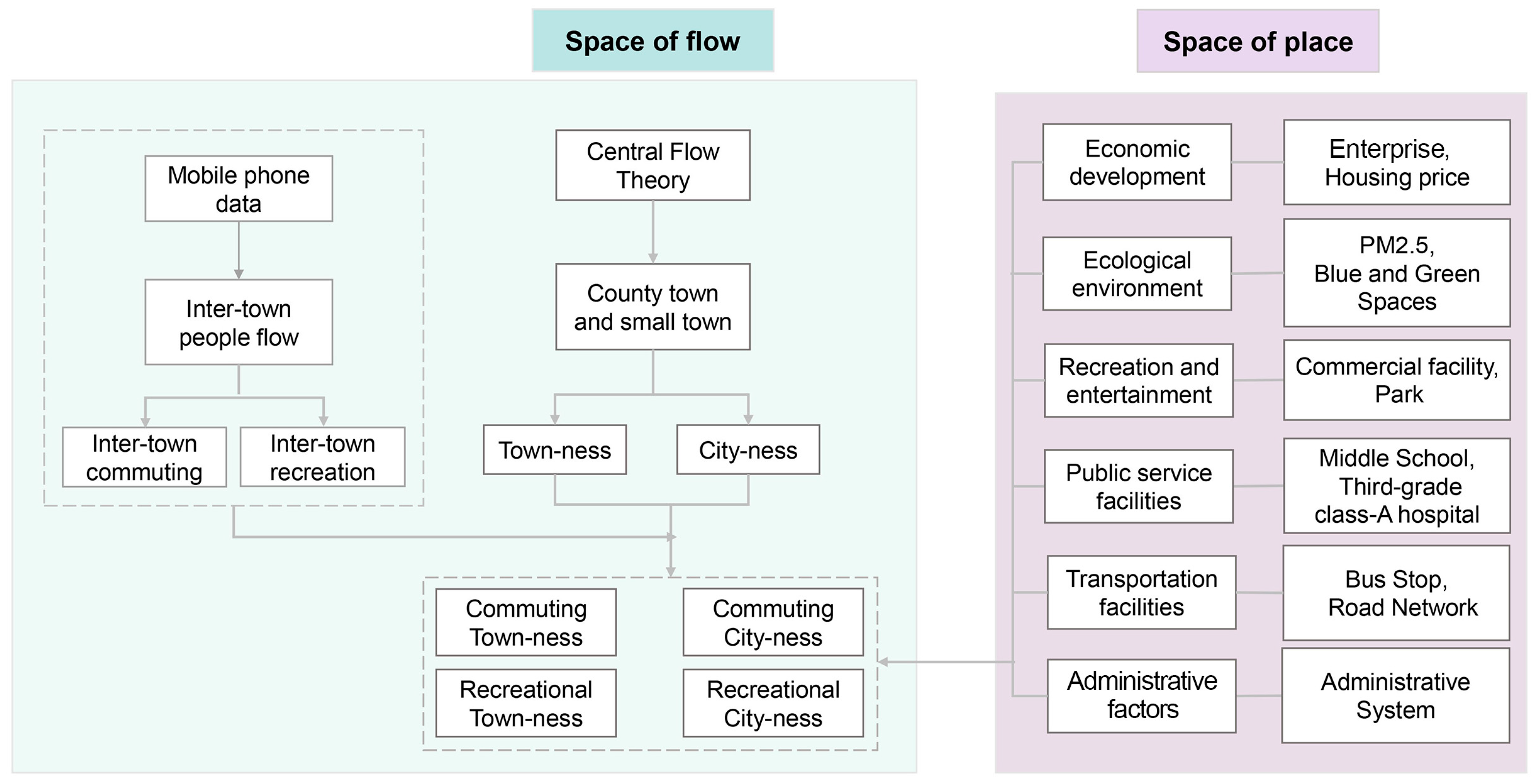
CFT holds that the flow of resources within the urban system is not detached from the space of places but interacts with the space of flows [2]. A large number of studies have confirmed that the built environment of the space of places affects the formation of the space of flows represented by capital and labor. This can be summarized as “urban attributes give rise to urban networks, and urban networks are rooted in urban attributes” [29]. It can be said that the generation of intertown people flows is influenced by the combined effect of the space of places, represented by the built environment of the town itself, including economic, social, environmental, and transportation factors. Therefore, the intertown people flows identified based on mobile phone data were used as the external relations of towns. To conduct an in-depth study of the spatial characteristics and influencing factors of the external relations of small towns categorized by function (commuting and recreation) and character (town-ness and city-ness), this research constructs an “Attribute-Network” conceptual framework (Figure 1).

Under the theoretical framework of “attribute-network”, we constructed a dataset focusing on categories of urban attributes: economic development, ecological environment, recreation and entertainment, public service facilities, transportation facilities, and administrative factors (Table 1). This dataset provides a comprehensive overview of urban attributes of 2331 towns in the YRD region. These variables are selected not merely as descriptive features but as theoretically grounded proxies that can be mapped onto commuting or recreational flows.

The influencing factors at the economic development level include enterprise density and housing prices [46,47]. High enterprise density is often associated with more job opportunities [48], which correlates with structural commuting flows. House prices are an important indicator reflecting the income level of residents. As a proxy for residents’ income and housing costs, on the one hand, they shape commuting networks by influencing residential location choices; on the other hand, the high consumption capacity implied by areas with high house prices also drives cross-boundary recreational flows.

Ecological factors include PM2.5 concentrations and the proportion of blue–green space. PM2.5 is often used to measure the degree of air pollution [49], which theoretically correlates with residential choices and recreational travel. The blue–green space ratio reflects the proportion of urban water bodies (blue space) and vegetation (green space) [50]. Towns with a higher proportion of blue–green space usually have a relatively better quality of living environment and attract more intertown recreational travel.

The density of commercial facilities and parks represents the factors influencing the level of recreational facilities. Theoretically, on the one hand, they can provide local service jobs, thereby generating commuting flows [51]; on the other hand, they are also core destinations for weekend consumption and recreation, which correlate with recreational flows [52].

Public service capabilities are measured by the density of middle schools and third-grade class-A hospitals. In China’s public service resource allocation system, middle schools and third-grade class-A hospitals are the primary representatives of public service capabilities [53]. At the same time, they align with both flow types [54,55]: as massive public institutions, they gather numerous professionals (e.g., medical staff and teachers), generating structured commuting flows. Concurrently, behaviors such as cross-regional medical visits or weekend visits to boarding students fall strictly under non-workplace and non-residence trips, effectively corresponding to recreational flows.

The influencing factors at the transportation facilities level include the density of bus stops and the density of the road network. Bus stops, as nodes of the public transportation system, directly affect residents’ travel patterns and the spatial range of daily activities [56]. At the same time, road network density has also been proven to significantly facilitate residents’ travel [57]. Both serve as infrastructural preconditions to overcome physical distances, enabling the realization of rigid daily commuting flows and elastic recreational flows.

Administrative factors mainly refer to administrative ranks. In the Chinese context, towns with higher administrative ranks tend to concentrate more social public resources, affecting regional employment (commuting) and service consumption (recreational), and consequently have a significant impact on residents’ travel [58].

Table 1. Data summary of the selected variables.

Category	Variable	Description	Unit	Data Sources
Economic development	X1 Enterprise	Number of enterprises per square kilometer.	count/km2	Bureau of Industry and Commerce.
	X2 Housing prices	Average housing price per square meter.	yuan/m2	Anjuke Platform. (https://anjuke.com)
Ecological environment	X3 PM2.5	Concentration of PM2.5 in the air.	μg/m3	The China High Air Pollutants (CHAP) dataset provided by the National Tibetan Plateau Science Data Center [59,60] (http://data.tpdc.ac.cn)
	X4 Blue and Green Space	Percentage of water and vegetation spaces.	%	Sentinel-2 imagery from the Copernicus Data Space Ecosystem. (https://dataspace.copernicus.eu)
Recreation and entertainment	X5 Commercial facility	Number of malls per square kilometer.	count/km2	Amap. (https://www.amap.com/)
	X6 Park	Number of parks per square kilometer.	count/km2
Public service facilities	X7 Middle School	Number of middle schools per square kilometer.	count/km2
	X8 Third-grade class-A hospital	Number of tertiary hospitals per square kilometer.	count/km2
Transportation facilities	X9 Bus Stop	Number of bus stops per square kilometer.	count/km2
	X10 Road Network	kilometers of roads per square kilometer.	km/km2
Administrative factors	X11 Administrative System	Two-tier System of County Seats and Small Towns	-	-

Table 1. Data summary of the selected variables.

Category	Variable	Description	Unit	Data Sources
Economic development	X1 Enterprise	Number of enterprises per square kilometer.	count/km2	Bureau of Industry and Commerce.
	X2 Housing prices	Average housing price per square meter.	yuan/m2	Anjuke Platform. (https://anjuke.com)
Ecological environment	X3 PM2.5	Concentration of PM2.5 in the air.	μg/m3	The China High Air Pollutants (CHAP) dataset provided by the National Tibetan Plateau Science Data Center [59,60] (http://data.tpdc.ac.cn)
	X4 Blue and Green Space	Percentage of water and vegetation spaces.	%	Sentinel-2 imagery from the Copernicus Data Space Ecosystem. (https://dataspace.copernicus.eu)
Recreation and entertainment	X5 Commercial facility	Number of malls per square kilometer.	count/km2	Amap. (https://www.amap.com/)
	X6 Park	Number of parks per square kilometer.	count/km2
Public service facilities	X7 Middle School	Number of middle schools per square kilometer.	count/km2
	X8 Third-grade class-A hospital	Number of tertiary hospitals per square kilometer.	count/km2
Transportation facilities	X9 Bus Stop	Number of bus stops per square kilometer.	count/km2
	X10 Road Network	kilometers of roads per square kilometer.	km/km2
Administrative factors	X11 Administrative System	Two-tier System of County Seats and Small Towns	-	-

3.2. Study Area

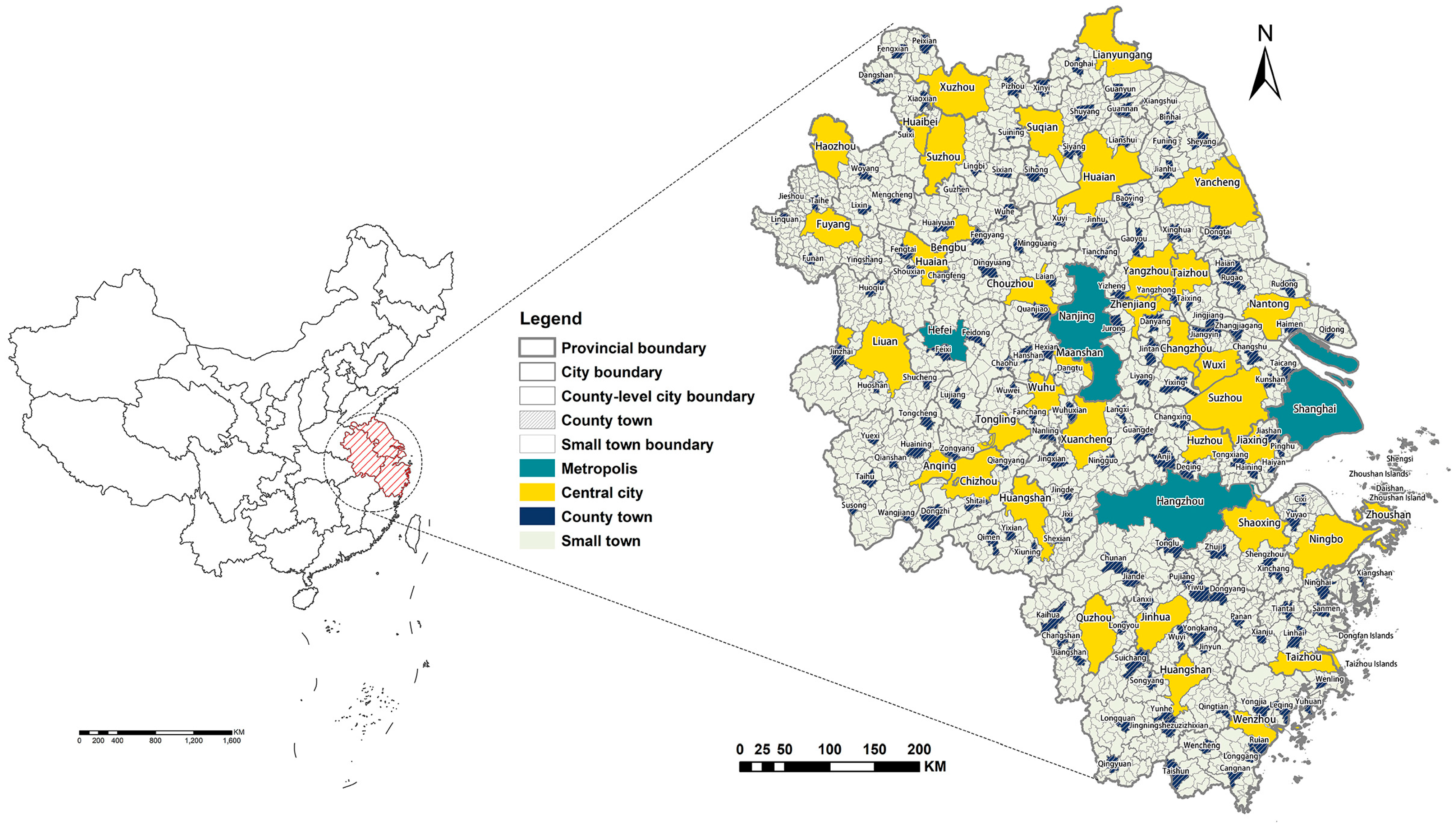
The study area is the YRD region of China. Based on China’s administrative hierarchy, the YRD region consists of 41 cities at the prefecture level and above, ranging from municipalities and provincial capitals to general prefecture-level cities. Prefecture-level cities include both municipal districts and county-level units, with the latter comprising county towns and small towns (see Figure 2). In this study, we refer to municipalities and provincial capitals collectively as “metropolises” and to municipal districts of the remaining cities as “central cities”. Thus, the YRD region encompasses four metropolises (Shanghai, Nanjing, Hangzhou, and Hefei), 37 central cities (such as Suzhou and Wuxi), 155 county towns, and 2176 small towns. Our primary focus is on the external relations of county towns and small towns.

3.3. Data and Methods

3.3.1. Mobile Phone Data to Identify People Flow

We utilized mobile phone data to analyze people flow in the YRD region as a proxy for external urban relations. Mobile phone data were obtained from China Unicom, one of the three major telecommunications operators in China. For this study, we collected mobile phone data over 31 days in December 2019, with strict measures in place to protect privacy: no personal information was included, and user locations were aggregated using a 1 km × 1 km grid. Given that mobility patterns were severely disrupted by major public health events between 2020 and 2023, the 2019 data can more accurately and objectively reflect the external relations of small towns under the combined effect of market mechanisms and built environments.

In addition, selecting December as the data window is highly appropriate. First, regarding commuting flows, December provides a very clear observation window. There are no statutory public holidays in China during December, which avoids the interference of large-scale travel associated with the National Day in October or the Spring Festival in January and February. Furthermore, December falls entirely within the normal academic semester, avoiding the impact of summer vacations (spanning from June to September) and winter vacations (from January to March), although specific dates vary among institutions. The mild winter climate in the subtropical YRD region experiences few extreme weather events, which minimizes the impact of climate variations on the structure of commuting mobility. Using single-month mobile phone data to characterize commuting patterns aligns with established practices in this field [61], further supporting the temporal validity of this approach. Second, regarding recreational flows, we acknowledge that outdoor recreational activities may decrease in December compared to spring or autumn. While seasonal fluctuations may affect the absolute volume of recreational trips and local spatial patterns (such as changes in the service radius of parks), they have a limited impact on the spatial heterogeneity mechanisms at the urban agglomeration scale, which is the core focus of this study.

Our analysis focuses on the spatiotemporal behavior of mobile phone users, allowing us to identify residences, workplaces, and recreational places. Using a relatively mature methodology [62], we classified external urban relations into three categories: commuting flows, recreational flows, and flows for other purposes. Although “flows for other purposes” were extracted in the initial classification, these flows are difficult to accurately distinguish and contain substantial data noise. Consequently, they fail to establish a clear functional attribution relationship with the built environment indicators selected in this study. Therefore, focusing on the employment and consumption activities that represent core urban functions, this paper only incorporates commuting and recreational flows into the final model analysis. The specific methods used in this study are as follows.

• Identification of home

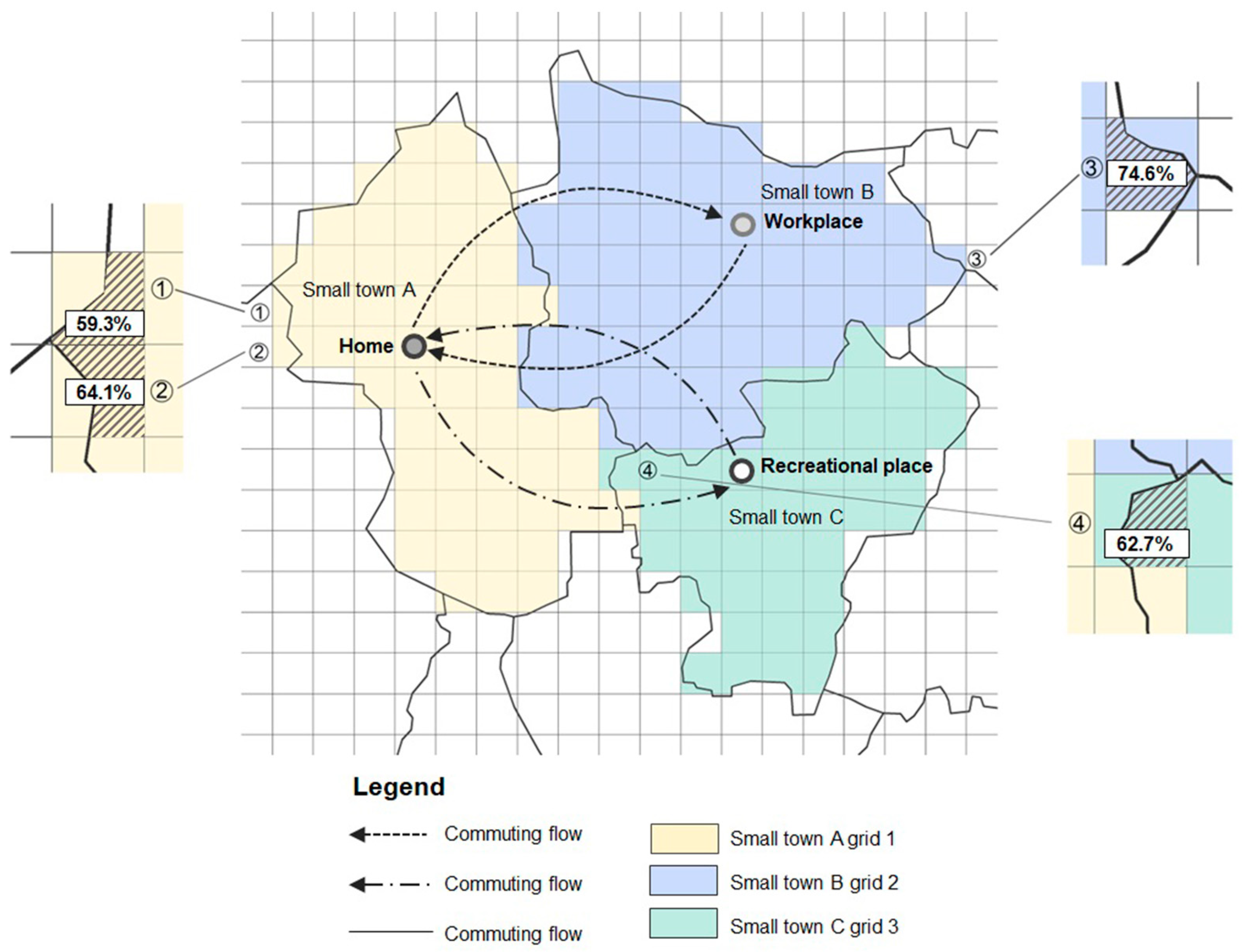
As illustrated in Figure 3, we first screened the base stations where users had a dwell time of at least 30 min between 23:00 and 5:00 and then selected the station with the longest nighttime dwell time as the user’s residence for that day. To determine their monthly residences, we used stations where the nighttime dwell time was the longest, and that appeared for more than 15 days (50% of the total days).

2.

Identification of workplace

We identified each user’s place of employment by screening the base stations where they spent the longest time, with a dwell time exceeding 30 min, between 9:00 and 17:00. Base stations with repeated long dwell times for more than 15 days were regarded as the user’s workplace in that month.

3.

Identification of recreational place

Excluding base stations identified as residences or workplaces, we classified base stations where users spent the longest time, with a dwell time exceeding 30 min, on non-working days as recreational places.

Figure 3 shows how the grid cells of the mobile phone data were aggregated to match the boundaries of county towns and small towns. We spatially matched the centroid of each grid cell with the boundary of the corresponding county town or small town (spatial unit) to ensure accurate data allocation. If a grid cell boundary did not perfectly coincide with a spatial unit, only grid cells with over 50% overlap were included, and each grid cell was assigned to only one spatial unit. Given that China Unicom users constitute approximately 20% of the total population, we scaled up the data to estimate the population flows. This process identified 127,990 daily commuting flows and 487,895 daily recreational flows in spatial units of the YRD region.

Figure 3. Schematic diagram of mobile phone data identifying home, workplace and recreational place.

Figure 3. Schematic diagram of mobile phone data identifying home, workplace and recreational place.

3.3.2. The Method for Defining the City-Ness and Town-Ness of People Flow Between County Towns and Small Towns

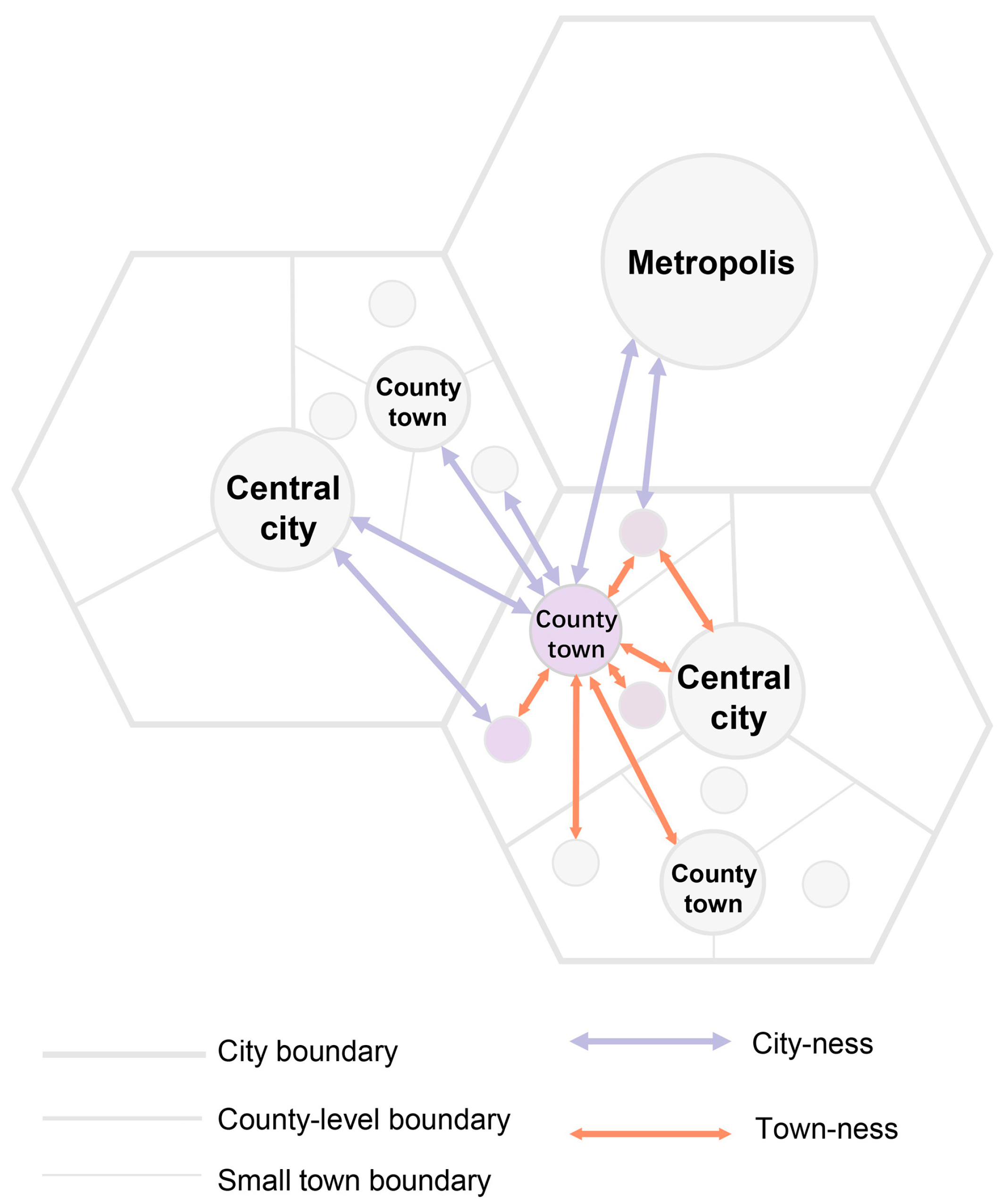
The delineation of “city-ness” and “town-ness” based on CFT hinges on the concept of the urban hinterland. Notably, there are no universally accepted criteria for defining urban hinterland boundaries. Although CPT conceptualizes the urban hinterland as an area within which high-level cities provide goods and public services, the extent of this area varies significantly depending on factors such as transportation modes and infrastructure, resulting in differing accessibility ranges over time. Unlike urban systems driven entirely by market forces, spatial development and resource allocation in Chinese cities are profoundly influenced by a top-down administrative hierarchy. Prefecture-level cities serve as key hubs for high-level commercial establishments, public service facilities, and major external transportation infrastructures, including airports and railway stations. These cities also facilitate connections between lower-tier towns within their hinterlands and offer higher-level commercial and business services; the transportation infrastructure further contributes to these functions [63].

The use of prefecture-level administrative boundaries as a proxy for urban hinterlands in this study is based not only on institutional factors but also on the real structural constraints that these boundaries impose on residents’ mobility. First, China’s household registration system links rights to public education, social insurance, and healthcare to specific administrative units, which substantially increases the cost of cross-boundary relocation [64], thereby concentrating daily activity spaces within prefecture-level cities. Second, Chinese administrative boundaries are the result of long-term historical evolution and are deeply aligned with natural topography and cultural identities [65]. Natural topography acts as a physical barrier to commuting, while culture (such as dialects) forms the community or psychological boundary for recreational, social, and economic activities.

Furthermore, methodologically, using administrative boundaries to delineate hinterlands offers comparative advantages. Common physical distance methods (such as isochrones or equidistant buffers) and gravity models have certain limitations. The physical distance method assumes a homogeneous space and fails to account for the real impacts of institutions and culture on people’s travel behavior. The classic gravity model heavily relies on the subjective definition of mass parameters (such as population and GDP), which not only introduces uncertainty in boundary delineation but also suffers from a similar lack of institutional and cultural considerations due to its distance parameter. Comparatively, while using administrative boundaries as proxies for hinterlands inevitably produces localized boundary effects, it effectively reflects the structure of urban spatial interactions.

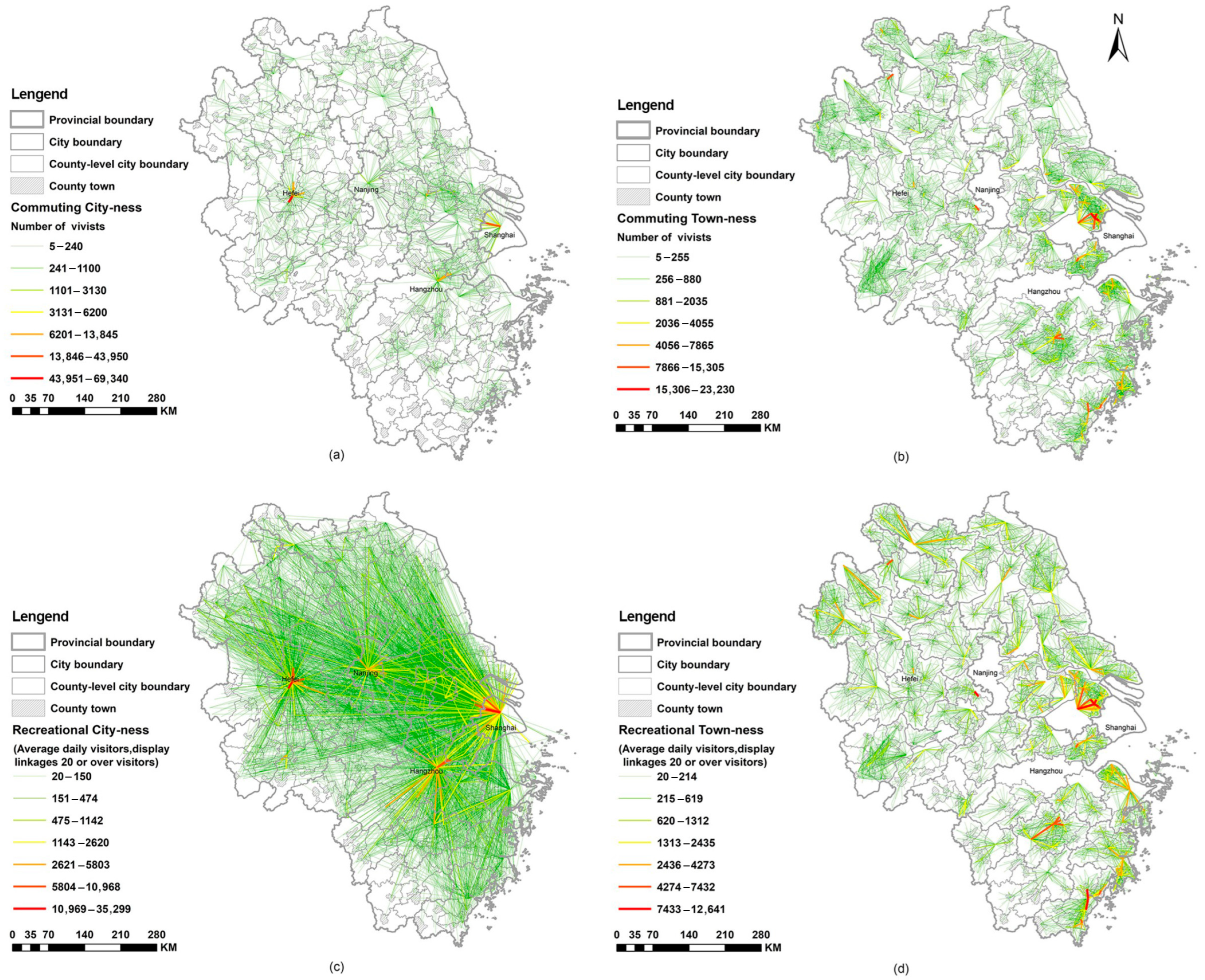
Based on this, we argue that China’s prefecture-level city administrative units meet CPT’s definition of an urban hinterland. Figure 4 illustrates how people flows within prefecture-level administrative units (central cities, county towns, and small towns) are classified as town-ness. Meanwhile, people flows between these areas and metropolises outside prefecture-level units are also regarded as city-ness. Figure 5 highlights the distinction between city-ness and town-ness based on external commuting and recreational flows in county towns and small towns within the YRD region. Notably, to analyze the external relations of towns, Figure 5 omits the people flows between metropolitan areas and central cities to focus on the flows of county towns and small towns.

3.3.3. Spatial Environmental Data

The dependent variables in this study were the four categories of commuting city-ness, commuting town-ness, recreational city-ness, and recreational town-ness, as described in Section 3.3.2. To ensure temporal consistency with the mobile phone signaling data collected in December 2019, all independent variables were sourced for the year 2019. The first set of independent variables pertains to economic development: data on the headquarters, branch offices, and subsidiaries of Fortune 500 companies were obtained from the Bureau of Industry and Commerce. Housing prices were determined using a Python (version 3.10) web scraping tool on the Anjuke website (https://anjuke.com). The second set of variables includes ecological, recreational, public, and transportation facilities, encompassing PM2.5 levels, blue–green space, commercial facilities, parks, middle schools, third-grade class-A hospitals, bus stops, and road network density. PM2.5 data were sourced from the CHAP dataset provided by the National Tibetan Plateau Science Data Center [59,60]. The proportion of blue–green space was calculated using Sentinel-2 imagery from the Copernicus Data Space Ecosystem (https://dataspace.copernicus.eu) by determining the ratio of the blue–green space area to the total area for each town. Data on the density of commercial facilities, parks, middle schools, third-grade class-A hospitals, and bus stops were collected using Python (version 3.10) to extract points of interest (POI) from Amap (https://www.amap.com/), a widely used mapping service in China. These densities were then calculated as the ratio of the POI counts to the total area of each town. Road network density was similarly derived using road data from Amap to calculate the ratio of the total road length to the town’s total area. The third set of variables considers the administrative factors that distinguish between county towns and small towns.

3.3.4. The Regression Analysis Method for Spatial Influencing Factors

To systematically investigate the spatial associations between the built environment and the external relations of small towns, we adopted a progressive analytical framework: advancing from spatial diagnostics and global baseline modeling to the MGWR model. Because the preliminary and comparative models applied in this study—including Global and Local Moran’s I, Ordinary Least Squares (OLS), the spatial autoregressive (SAR) model, the spatial error model (SEM), and standard Geographically Weighted Regression (GWR)—are standard spatial econometric tools, their detailed formulations are widely documented in classical spatial literature [29,66,67,68,69,70,71,72] and are thus omitted here. The subsequent sections detail the diagnostic progression and the specific mathematical formulation of the MGWR model.

• Spatial autocorrelation and baseline diagnostics

Initially, Global Moran’s I and Local Moran’s I, Local Indicators of Spatial Association (LISA), were employed to measure the overall clustering and identify localized spatial association patterns of the four types of external relations [70]. Subsequently, an OLS model was constructed as a non-spatial baseline. To rigorously validate the OLS assumptions, the Breusch–Pagan and Koenker–Bassett tests were conducted to detect spatial heteroskedasticity [44], and Lagrange multiplier (LM) tests were utilized to diagnose spatial dependence in the residuals [71].

2.

Global spatial models (SAR and SEM)

Upon detecting significant global spatial autocorrelation via the LM tests, the SAR and SEM were introduced as intermediate benchmarks [71]. The SAR model controls for spatial spillover effects among neighboring towns (spatial lag), while the SEM accounts for spatial dependence operating through unobserved, spatially correlated error terms (spatial error) [44,71].

3.

Multiscale geographically weighted regression (MGWR)

While SAR and SEM effectively control for global spatial dependence, they assume spatially constant relationships. To address the localized non-stationarity confirmed by the heteroskedasticity diagnostics, the MGWR model was ultimately employed. The MGWR model extends GWR by allowing spatially varying relationships at multiple scales, offering a more refined approach for modeling spatial heterogeneity [73]. Previous studies have applied the MGWR model to national-level research [74] and urban agglomerations [75] in the context of regional urbanization, making it suitable for this study. The formula for MGWR is as follows:

$$y_i={\beta }_0\left(u_i,v_i\right)+\sum _{k=1}^m{\beta }_k\left(u_i,v_i;{\theta }_k\right)x_{ik}+{ϵ}_i$$

(1)

where $\left(u_i,v_i\right)$denotes the spatial coordinates of town i; $x_{ik}$is the value of the $k$-th independent variable at location i; ${\beta }_k\left(u_i,v_i;{\theta }_k\right)$ represents the local regression coefficient for the $k$-th independent variable at location i, with ${\theta }_k$ indicating the variable-specific optimal bandwidth; and ${ϵ}_i$ is the random error term.

4. Results

4.1. Spatial Patterns of External Relations of Towns

The spatial autocorrelation patterns of commuting and recreational flows of county towns and small towns in the study area are crucial for subsequent spatial modeling. Therefore, global Moran’s I was computed for the four types of external relations of towns: commuting town-ness, commuting city-ness, recreational town-ness and recreational city-ness. The resulting values were 0.0954, 0.4770, 0.2389, and 0.4818, with corresponding Z-values of 16.7290, 72.9147, 38.9699, and 72.1331, respectively. All metrics demonstrated highly significant positive spatial autocorrelation (p < 0.05). These results indicate a significant spatial autocorrelation for both commuting and recreational flows, necessitating further analysis of spatial heterogeneity.

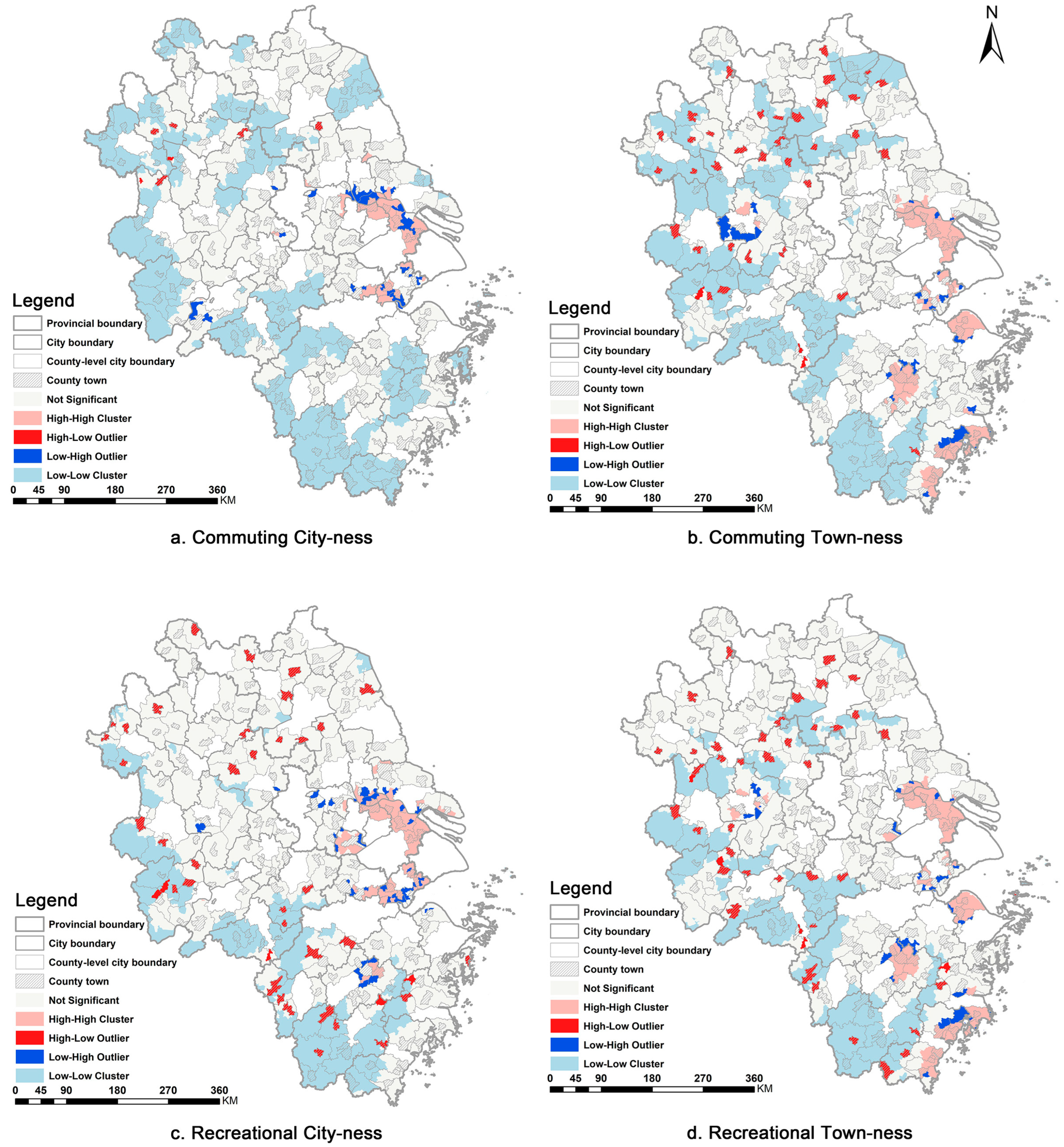
We further applied Local Moran’s I to investigate the spatial autocorrelation of commuting city-ness, commuting town-ness, recreational city-ness, and recreational town-ness. Figure 6 shows that high–high clustering areas were concentrated in economically developed county towns and small towns in cities such as Shanghai, Hangzhou, Suzhou, and Wuxi in the eastern YRD region. In contrast, high–low clustering areas were more dispersed and were mainly located in smaller towns in the northern, western, and southern YRD regions. The low–high clustering areas were mainly towns on the outskirts of metropolitan regions, indicating that towns within metropolitan areas have a relatively clear advantage in the volume of people flow. Low–low clustering areas were predominantly found in the mountainous southwestern and agricultural northeastern regions of the YRD.

Overall, while the four types of external relations exhibited similar broad spatial patterns, they also displayed significant localized differences. These differences highlight the distinct characteristics of commuting flows and recreational flows, as well as the varying distances between trips categorized as city-ness and town-ness.

4.2. Results of OLS, SAR, SEM, GWR, and MGWR Models

4.2.1. Preliminary Selection of Influencing Factors

During model specification, explanatory variables may exhibit multicollinearity, which can compromise the validity of statistical inferences. To mitigate this issue, a variance inflation factor (VIF) test was conducted. Variables with a VIF exceeding 5 were excluded, resulting in the retention of 11 independent variables [76] (Table 2). The mean VIF for the retained variables was 2.11, indicating minimal multicollinearity. The maximum VIF was observed for X₆ (VIF = 3.06), indicating that there is no collinearity problem among the independent variables.

Further statistical diagnostics were conducted to test the assumptions of the traditional regression model. The Breusch–Pagan (BP) and Koenker–Bassett (KB) tests yielded p-values of 0.00 across all four types of external relations, indicating severe spatial heteroskedasticity in the data. Additionally, Moran’s I values of the OLS residuals were highly significant (p < 0.01). The Lagrange multiplier tests (LM-Lag and LM-Error) and their robust counterparts generally showed high significance (p < 0.01), confirming the presence of significant spatial dependence, encompassing both spatial lag and spatial error effects. These diagnostic results demonstrate that traditional OLS estimation violates classical assumptions in this context, necessitating the use of spatial regression models that can simultaneously account for spatial dependence and spatial heterogeneity.

Figure 6. LISA of external relations of small towns in the YRD region.

Figure 6. LISA of external relations of small towns in the YRD region.

Table 2. VIF test of influencing factors.

Variable	VIF
X1 Enterprise	1.37
X2 Housing prices	1.69
X3 PM2.5	1.39
X4 Blue and Green Spaces	1.45
X5 Commercial facility	2.54
X6 Park	3.06
X7 Middle School	2.59
X8 Tertiary Hospitals	2.88
X9 Bus Stop	2.74
X10 Road Network	1.24
X11 Administrative System	2.26

Table 2. VIF test of influencing factors.

Variable	VIF
X1 Enterprise	1.37
X2 Housing prices	1.69
X3 PM2.5	1.39
X4 Blue and Green Spaces	1.45
X5 Commercial facility	2.54
X6 Park	3.06
X7 Middle School	2.59
X8 Tertiary Hospitals	2.88
X9 Bus Stop	2.74
X10 Road Network	1.24
X11 Administrative System	2.26

4.2.2. Comparison of OLS, SAR, SEM, GWR, and MGWR Models

Spatial autocorrelation, heteroskedasticity, and non-stationarity were confirmed across the four types of external relations of small towns. Consequently, the SAR, SEM, GWR and MGWR models were employed to explore the spatial associations and their non-stationary patterns. As shown in

Table 3. Overall performance of all models.

Dependent Variables		Model Goodness-of-Fit
		RSS	AICC	Adj. R2	Pseudo-R2
Commuting City-ness	OLS	1898.921	6163.367	0.181	-
	SAR	1877.609	6145.012	-	0.195
	SEM	1899.700	6136.043	-	0.185
	GWR	432.840	3747.789	0.814	-
	MGWR	355.433	3028.962	0.822	-
Commuting Town-ness	OLS	1231.038	5153.046	0.469	-
	SAR	887.214	4485.857	-	0.620
	SEM	1309.388	4475.731	-	0.450
	GWR	424.052	3760.900	0.775	-
	MGWR	375.769	3217.014	0.809	-
Recreational City-ness	OLS	1458.038	5547.530	0.372	-
	SAR	1328.452	5375.768	-	0.431
	SEM	1390.388	4475.731	-	0.371
	GWR	516.015	4028.115	0.735	-
	MGWR	405.631	3310.615	0.797	-
Recreational Town-ness	OLS	888.722	4393.540	0.617	-
	SAR	603.969	3586.957	-	0.741
	SEM	962.390	3538.477	-	0.600
	GWR	327.960	3031.812	0.830	-
	MGWR	279.786	2502.412	0.859	-

, the SAR and SEM improved the model performance over the OLS approach by capturing global spatial dependence, evidenced by increased R² and decreased AICc values. However, the local spatial models (GWR and MGWR) yielded vastly superior improvements. While standard GWR improves upon global models, it imposes a uniform bandwidth, implicitly assuming all spatial factors operate at the same scale. This assumption is misspecified for this study, as variables operate at fundamentally different scales. By allowing spatially varying relationships at multiple scales, MGWR overcomes this limitation. For instance, the AICc values of the MGWR model for commuting city-ness, commuting town-ness, recreational city-ness, and recreational town-ness dropped significantly to 3028.962, 3217.014, 3310.615, and 2502.412, respectively. These values are substantially lower than those of the SAR, SEM, and standard GWR models. This comparative analysis provides robust statistical and theoretical evidence that while global spatial spillover effects (spatial lag and error) exist, the spatial non-stationarity (heterogeneity) in the relationships between spatial factors and external relations provides substantially higher explanatory power for the external relations of small towns. Consequently, these findings demonstrate that by accommodating scale-specific local properties in spatial data, the MGWR model represents the minimum appropriate specification for uncovering the complex spatial associations in this study.

4.2.3. Scale Analysis of the MGWR Model

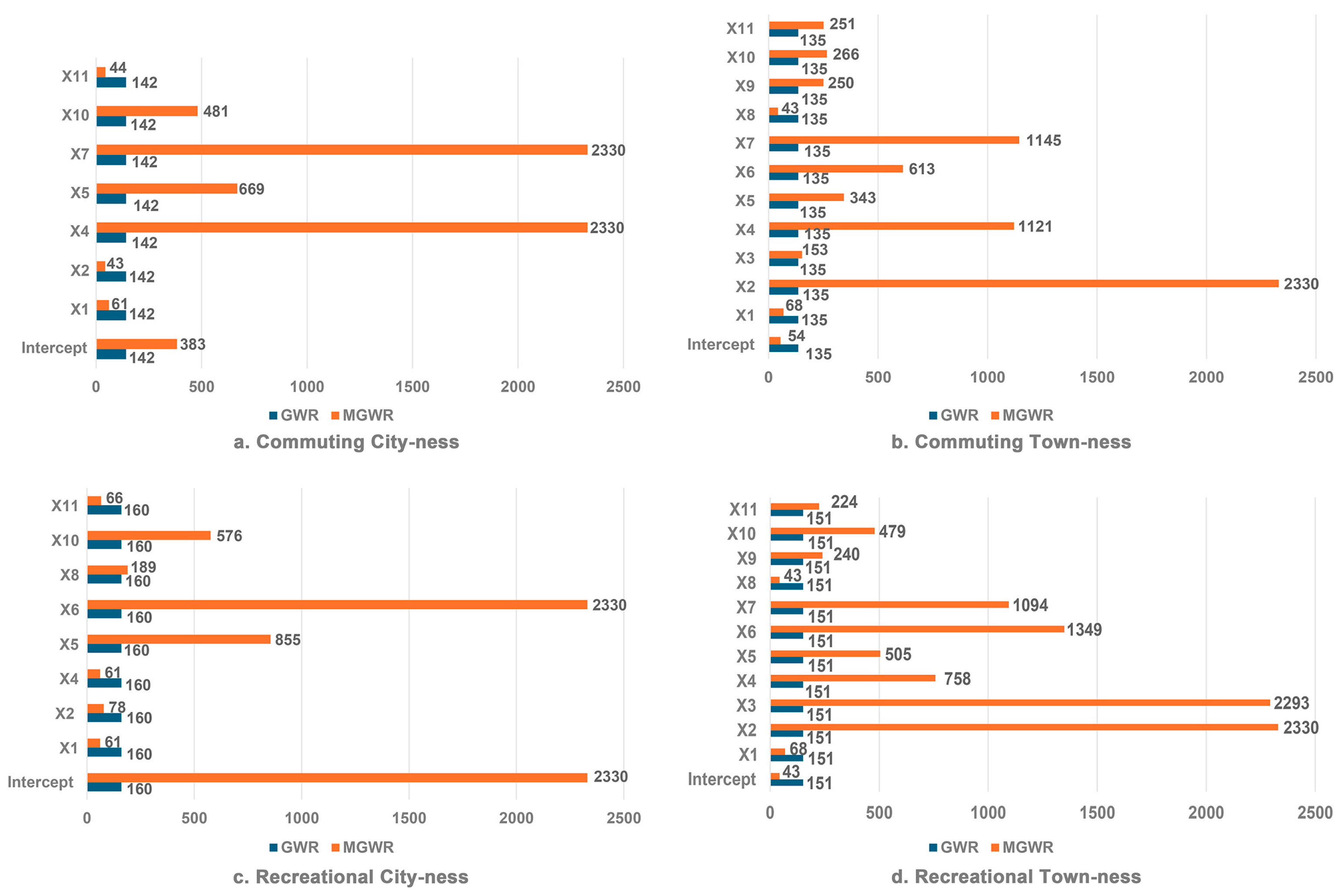
In the MGWR scale analysis, the spatial heterogeneity of the associations between independent variables is inversely related to their bandwidths; specifically, a larger bandwidth indicates lower spatial heterogeneity.

Figure 7a illustrates that the bandwidths for blue–green space (X₄) and middle schools (X₇) are 2330, approaching the global scale (n = 2331). This indicates that the effects of these two variables on commuting city-ness are relatively stable across space, exhibiting minimal spatial heterogeneity. In contrast, the bandwidths of enterprise density (X₁), housing price (X₂), and administrative factors (X₁₁) are 61, 43, and 44, respectively. These relatively small values suggest greater spatial heterogeneity in their spatial relationships with commuting city-ness. Similarly, Figure 7b demonstrates minimal spatial heterogeneity in the effects of housing price (X₂), blue–green space (X₄), and middle schools (X₇) on commuting town-ness, with bandwidths of 2330, 1121, and 1145, respectively. However, enterprise density (X₁) and third-grade class-A hospitals (X₈) exhibit high spatial heterogeneity (bandwidth = 68 and 43, respectively). In Figure 7c, park (X₆), which operates on a near-global scale (bandwidth = 2330), exhibits a relatively homogeneous spatial association with recreational city-ness. Conversely, enterprise density (X₁), housing price (X₂), blue–green space (X₄), and administrative factors (X₁₁) exhibit significant spatial heterogeneity (bandwidths = 61, 78, 61, and 66, respectively), with their effects on recreational city-ness varying across regions. Finally, in Figure 7d, there is minimal spatial heterogeneity in the effects of housing price (X₂), PM2.5 (X₃), parks (X₆), and middle schools (X₇) on recreational town-ness, as evidenced by their large bandwidths (2330, 2293, 1349, and 1094, respectively). However, enterprise density (X₁) and third-grade class-A hospitals (X₈) display high spatial heterogeneity (bandwidths = 68 and 43, respectively), closely resembling the patterns observed for commuting town-ness.

4.3. Unpacking Spatial Non-Stationarity of City-Ness and Town-Ness

4.3.1. Spatial Non-Stationarity of Commuting City-Ness

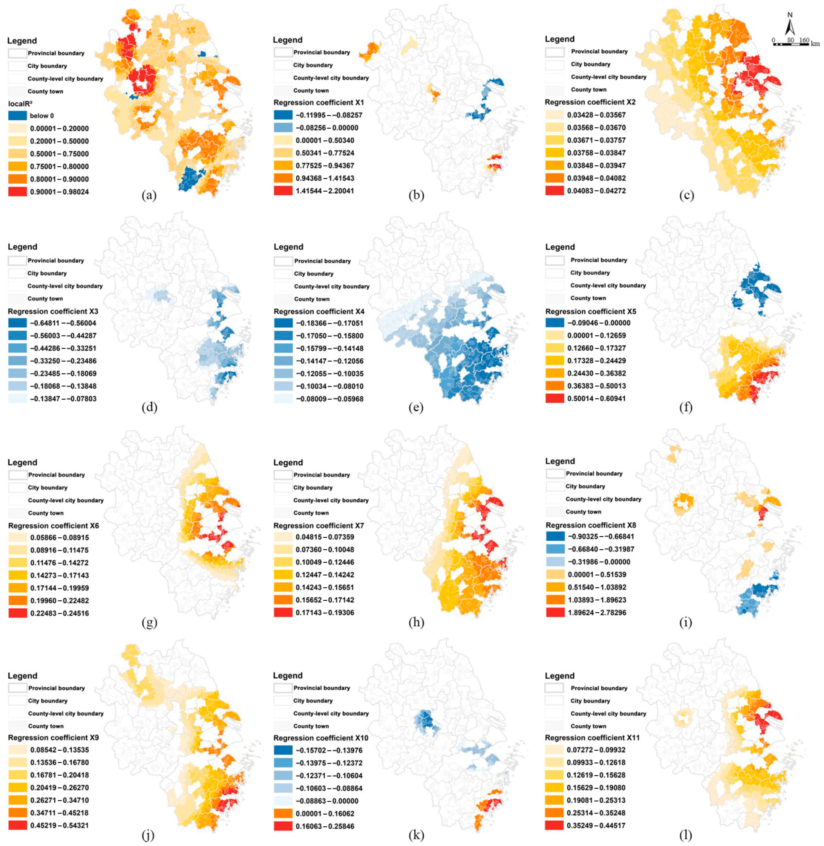
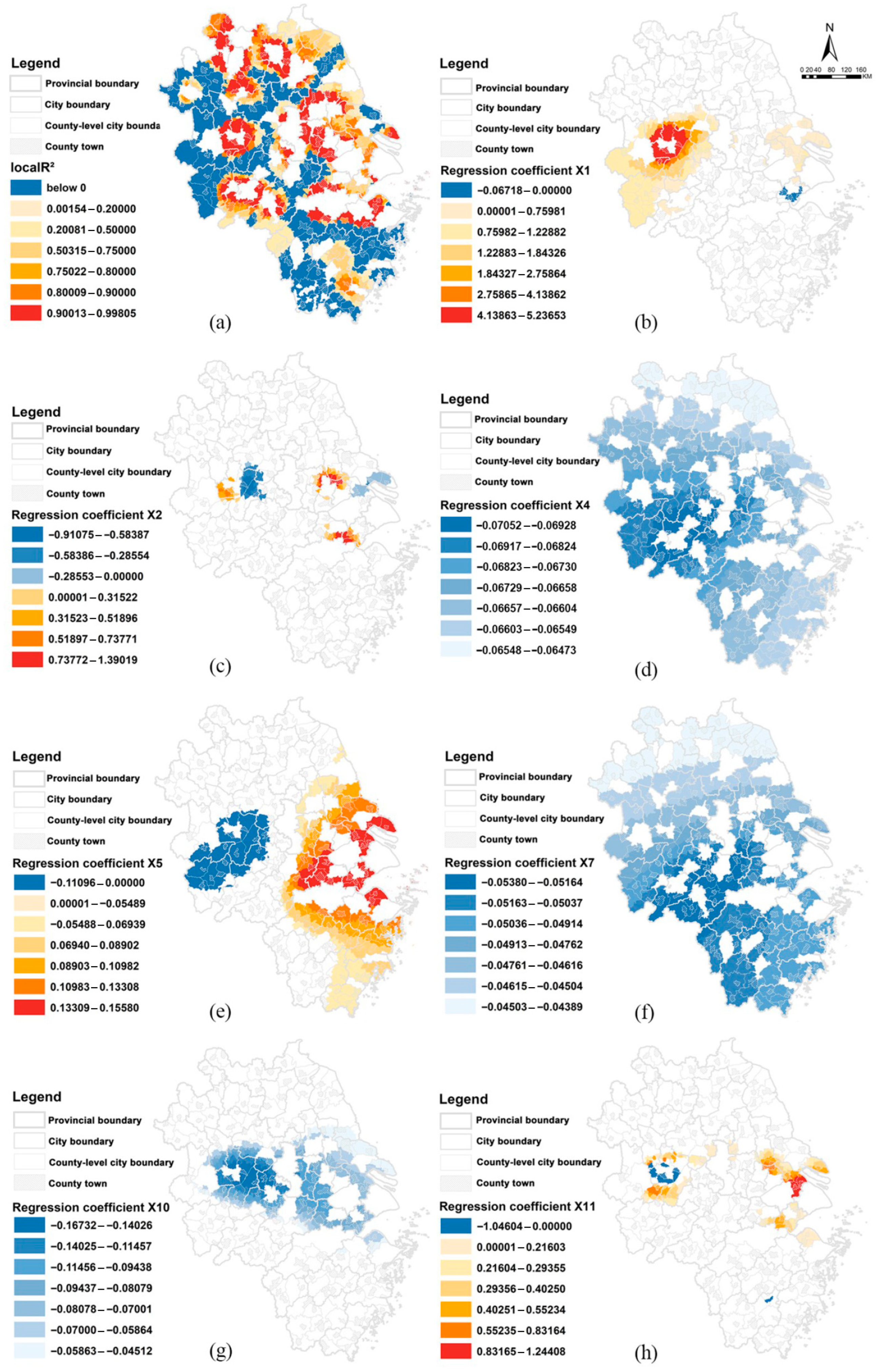
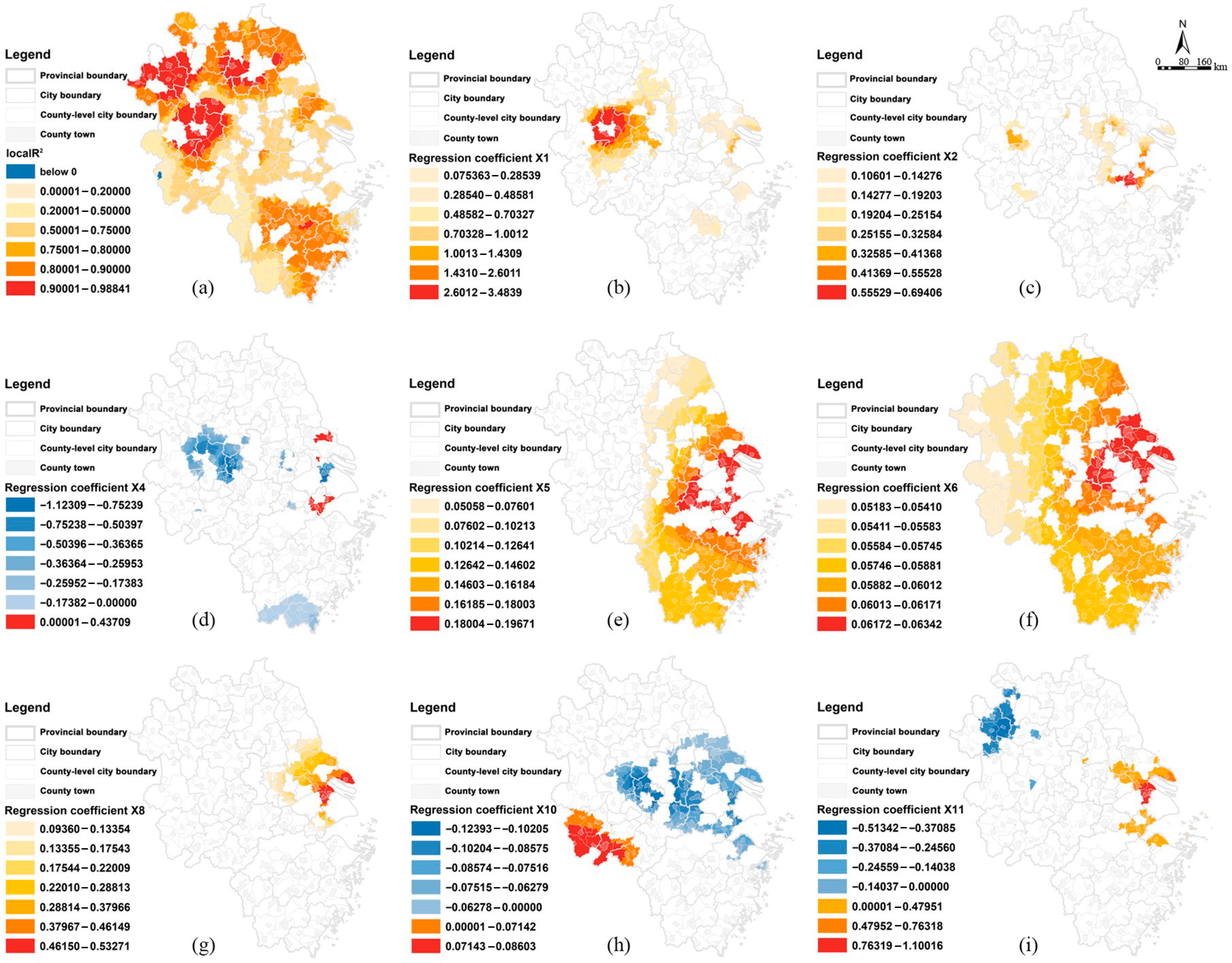
Figure 8 shows the regression coefficients for commuting city-ness in county towns and small towns within the YRD region, as calculated using the MGWR model across different evaluation indicator systems. Among the 11 independent variables, seven yielded p-values < 0.05, demonstrating statistical significance. Figure 8a presents the spatial distribution of local R² values, reflecting the explanatory capacity of the model across geographic regions. A local R² greater than 0.75 suggests strong model explanatory capacity, while a value below 0.5 indicates weaker explanatory capacity. Spatially, the local R² distribution exhibited significant heterogeneity, with metropolitan areas and most towns surrounding central cities showing values above 0.75. The proportion of towns with local R² values exceeding 0.50 reached 32.9%.

Enterprise density (X₁) had the strongest association among all the variables, as indicated by the absolute values of the regression coefficients (Figure 8b). The results revealed a positive relationship between enterprise density and commuting city-ness in towns surrounding the Hefei and Shanghai metropolitan areas. In contrast, the relationship in towns near Jiaxing was negative, reflecting that higher enterprise density in this subregion is associated with lower levels of commuting city-ness.

Housing prices (X₂) also exhibited significant spatial variation (Figure 8c). Housing prices were positively correlated with commuting city-ness in the areas surrounding Hangzhou, Changzhou, and parts of Hefei, whereas a negative relationship was observed in some parts of Nantong and other parts of Hefei.

The ecological environment, represented by the proportion of blue–green space (X₄), exhibited a negative association with commuting city-ness (Figure 8d). Its bandwidth approached the global scale, indicating minimal spatial variation in its association. From the absolute value of regression coefficients, the proportion of blue–green space had the weakest correlation with commuting city-ness.

The density of commercial facilities (X₅) exhibited markedly different spatially varying relationships with the commuting city-ness patterns across various areas of the YRD region (Figure 8e). In the developed eastern coastal areas, commercial density was positively correlated with commuting city-ness, while the opposite was observed in the western parts of the region.

Middle school density (X₇) showed a relatively weak negative association with commuting city-ness (Figure 8f) with a near-global bandwidth. Road network density (X₁₀) showed a weak negative association with commuting city-ness (Figure 8g). Furthermore, the results revealed that the positive association of administrative level (X₁₁) between commuting city-ness in the Yangtze River Delta was restricted to the neighboring towns of the four core cities of Shanghai, Hangzhou, Nanjing and Hefei, while the remaining regions exhibited negative or negligible associations (Figure 8h).

4.3.2. Spatial Non-Stationarity of Commuting Town-Ness

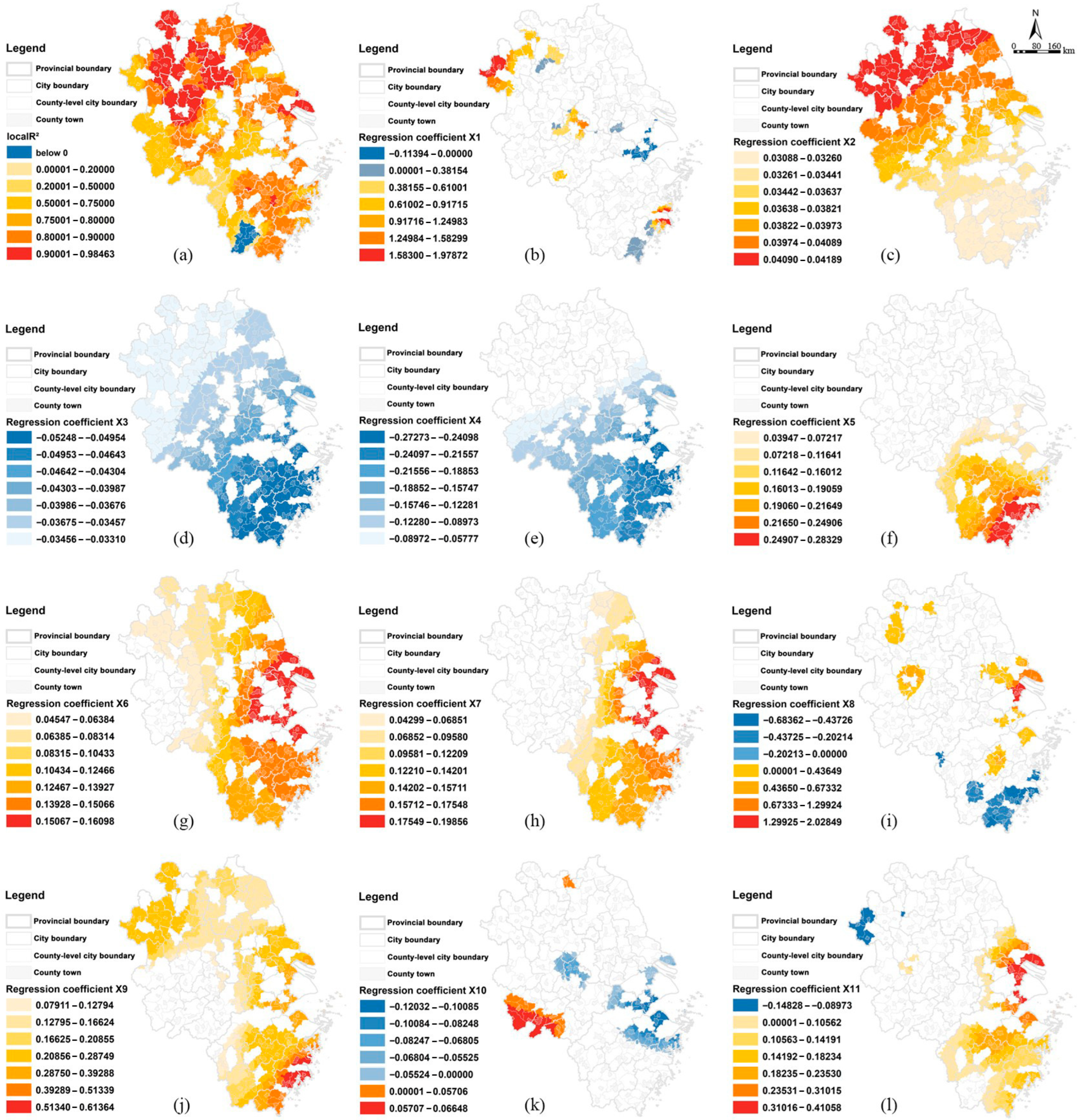
Figure 9 presents the regression coefficients of commuting town-ness for county towns and small towns in the YRD region, estimated using the MGWR model. The p-values for all 11 independent variables were below 0.05, indicating statistical significance. Figure 9a shows that 78.42% of towns had local R² values above 0.5, with 38.82% exceeding 0.75. Regions with high local R² values were primarily concentrated in less developed towns in the central and northern parts of Anhui and in the central and southern parts of Zhejiang, which contrasted with the spatial pattern observed in Figure 8a.

Enterprise density (X₁) was positively correlated with commuting town-ness in only a few towns located in the peripheral areas of the YRD region, far from the core metropolises. In contrast, towns near Shanghai and Hangzhou showed a negative relationship. Housing prices (X₂) exhibited a relatively weak positive relationship with commuting town-ness (Figure 9c). The bandwidth of housing prices (2330) approached the global scale, indicating that the relationship between housing costs and commuting town-ness was spatially stable across the region.

Figure 8. Spatial patterns of regression coefficient of commuting city-ness: (a) local R2; (b) enterprise density (X₁); (c) housing prices (X₂); (d) blue–green space (X₄); (e) commercial facilities (X₅); (f) middle school density (X₇); (g) road network density (X₁₀); (h) administrative level (X₁₁).

Figure 8. Spatial patterns of regression coefficient of commuting city-ness: (a) local R2; (b) enterprise density (X₁); (c) housing prices (X₂); (d) blue–green space (X₄); (e) commercial facilities (X₅); (f) middle school density (X₇); (g) road network density (X₁₀); (h) administrative level (X₁₁).

PM2.5 concentrations (X₃) exhibited a weak negative association with commuting town-ness in the southeastern YRD (Figure 9d). Similar to its association with commuting city-ness, the blue–green space share (X₄) demonstrated a relatively large regional bandwidth (1121), exhibiting a weak negative association with commuting town-ness across nearly half of the study area (Figure 9e).

The density of commercial facilities (X₅) exerted a more pronounced and spatially concentrated influence on commuting town-ness than on commuting city-ness (Figure 9f). Specifically, a distinct positive association was concentrated in the southern YRD (primarily Zhejiang province), contrasting sharply with a negative association observed in the northern regions. Park density (X₆) showed a relatively weak positive correlation with commuting town-ness (Figure 9g). The positive correlation of X6 was primarily observed in the eastern areas of the YRD region.

Middle school density (X₇), with a bandwidth (1145) indicating regional-scale stability, exhibited a relatively weak positive association with commuting town-ness. This pattern contrasted with the results for commuting city-ness. As another public service indicator, third-grade class-A hospital density (X₈) exhibited geographical variation in its relationship with commuting town-ness. In the areas surrounding the metropolitan regions of Shanghai and Hefei, X₈ was positively correlated with commuting town-ness. Conversely, negative relationships were observed in towns surrounding Wenzhou and Taizhou.

Bus stop density (X₉) exhibited a weaker positive relationship with commuting town-ness, predominantly in the eastern, southern, and north-central YRD regions (Figure 9j). Road network density (X₁₀) had a limited and geographically varied association with commuting town-ness. While a distinct positive relationship was observed in southern towns near Taizhou and Wenzhou, a contradictory negative relationship emerged in the central-western towns of the YRD.

Finally, administrative factors (X₁₁) had a relatively weak positive correlation with commuting town-ness, primarily in the eastern and southern parts of the YRD region (Figure 9l).

Figure 9. Spatial patterns of regression coefficient of commuting town-ness: (a) local R2; (b) enterprise density (X₁); (c) housing prices (X₂); (d) PM2.5 concentrations (X₃); (e) blue–green space (X₄); (f) commercial facilities (X₅); (g) park density (X₆); (h) middle school density (X₇); (i) third-grade class-A hospital density (X₈); (j) bus stop density (X₉); (k) road network density (X₁₀); (l) administrative level (X₁₁).

Figure 9. Spatial patterns of regression coefficient of commuting town-ness: (a) local R2; (b) enterprise density (X₁); (c) housing prices (X₂); (d) PM2.5 concentrations (X₃); (e) blue–green space (X₄); (f) commercial facilities (X₅); (g) park density (X₆); (h) middle school density (X₇); (i) third-grade class-A hospital density (X₈); (j) bus stop density (X₉); (k) road network density (X₁₀); (l) administrative level (X₁₁).

4.3.3. Spatial Non-Stationarity of Recreational City-Ness

Figure 10 presents the regression coefficients for recreational city-ness in county towns and small towns in the YRD region, as measured by the MGWR model. Among the 11 independent variables examined, eight variables had p-values below 0.05, demonstrating statistical significance. Figure 10a shows that 88.20% of the towns have local R² values greater than 0.5, with 61.43% exceeding 0.75. Spatially, these high explanatory powers were primarily concentrated in towns in northern Jiangsu, northern and central Anhui, and central and southern Zhejiang within the YRD region.

Among all independent variables, enterprise density (X₁) exerted the most pronounced positive association with recreational city-ness (Figure 10b). The magnitude of this positive association exhibited distinct spatial heterogeneity. The highest coefficients clustered around the Hefei metropolitan area, whereas eastern coastal regions near Shanghai showed a marginal positive relationship. Housing prices (X₂) also revealed a positive correlation with recreational city-ness, especially in towns surrounding metropolitan areas such as Shanghai, Nanjing, Hangzhou, and Hefei (Figure 10c).

The proportion of blue–green space (X₄) demonstrated spatially heterogeneous relationships with recreational city-ness. As illustrated in Figure 10d, this variable exhibited a predominantly negative correlation with recreational city-ness across the majority of the study area. Conversely, a positive correlation emerged in towns surrounding Jiaxing and Nantong.

The density of commercial facilities (X₅) exhibited pronounced spatial heterogeneity in its association with recreational city-ness (Figure 10e). Specifically, a strong positive correlation was observed in towns surrounding major metropolises like Shanghai and Hangzhou, whereas this positive correlation diminished significantly in the northern Jiangsu region.

Operating at a near-global scale (bandwidth = 2330, n = 2331), park density (X₆) showed a relatively weak but universally positive correlation with recreational city-ness across the study area. Figure 10f shows that park density had the strongest association with recreational city-ness in the eastern regions of the YRD.

The density of third-grade class-A hospitals (X₈) had a significant positive correlation with recreational city-ness, particularly in towns around the Shanghai metropolitan area (Figure 10g). A distinct distance-decay pattern was observed, where the strength of this positive correlation intensified in closer proximity to Shanghai.

Road network density (X₁₀) exhibited pronounced spatial non-stationarity in its relationship with recreational city-ness (Figure 10h). It demonstrated a negative correlation across the central and eastern portions of the YRD, contrasting with a distinct positive correlation observed in the southwestern peripheral towns. Administrative factors (X₁₁) had a positive correlation concentrated in towns surrounding the Shanghai metropolitan area on the eastern coast, whereas a pronounced negative association emerged in the northwestern towns of the YRD.

4.3.4. Spatial Non-Stationarity of Recreational Town-Ness

Figure 11 illustrates the regression coefficients for recreational town-ness in county towns and small towns across the YRD, as estimated by the MGWR model. The p-values of all 11 independent variables were below 0.05, indicating statistical significance. Figure 11a shows that 92.75% of towns had local R² values exceeding 0.5, while 71.77% had R² values greater than 0.75, indicating enhanced model explanatory power compared to the recreational city-ness.

Figure 11b highlights the association between enterprise density (X₁) and recreational town-ness in the YRD region. Unlike its association with recreational city-ness, the spatial relationship between X₁ and recreational town-ness shows no clear spatial regularity. Operating at a near-global scale (bandwidth = 2300, n = 2331), housing prices (X₂) exhibited a relatively weak positive association with recreational town-ness (Figure 11c). Compared to recreational city-ness, housing prices demonstrated a more extensive spatial correlation with recreational town-ness. This positive association was particularly robust in the northwestern YRD.

Operating at a near-global scale (bandwidth = 2293, n = 2331), PM2.5 concentration (X₃) exhibited a weak negative association with recreational town-ness (Figure 11d). This result confirms that environmental quality exerts a broader spatial correlation with recreational town-ness than with commuting town-ness. This negative association diminished in the northern YRD region, where the regression coefficients approached zero.

The proportion of blue–green space (X₄) exhibited a weak negative association with recreational town-ness, with its spatial distribution of coefficients clearly demarcated by a boundary along the Yangtze River. This negative relationship was predominantly concentrated in the southern portion of the YRD region, while the correlation remained negligible in the northern areas (Figure 11e).

The density of commercial facilities (X₅) exhibited a weak positive association with recreational town-ness, particularly in the Wenzhou and Taizhou areas of the southern YRD region (Figure 11f). Compared to its association with recreational city-ness, the correlation of commercial facilities with recreational town-ness was more geographically constrained. With a bandwidth (1349, n = 2331) indicating regional-scale stability, park density (X₆) was positively associated with recreational town-ness. Its spatial distribution was closely aligned with the patterns observed for recreational city-ness.

Figure 11. Spatial patterns of regression coefficient of recreational town-ness: (a) local R2; (b) enterprise density (X₁); (c) housing prices (X₂); (d) PM2.5 concentrations (X₃); (e) blue–green space (X₄); (f) commercial facilities (X₅); (g) park density (X₆); (h) middle school density (X₇); (i) third-grade class-A hospital density (X₈); (j) bus stop density (X₉); (k) road network density (X₁₀); (l) administrative level (X₁₁).

Figure 11. Spatial patterns of regression coefficient of recreational town-ness: (a) local R2; (b) enterprise density (X₁); (c) housing prices (X₂); (d) PM2.5 concentrations (X₃); (e) blue–green space (X₄); (f) commercial facilities (X₅); (g) park density (X₆); (h) middle school density (X₇); (i) third-grade class-A hospital density (X₈); (j) bus stop density (X₉); (k) road network density (X₁₀); (l) administrative level (X₁₁).

With a bandwidth (1049, n = 2331) indicating regional-scale stability, middle school density (X₇) showed a weak positive association with recreational town-ness. Similarly, the spatial pattern of correlation for hospital density (X₈) on recreational town-ness as a public service facility resembles its association with commuting town-ness (Figure 11i). As shown in Figure 11i, its local coefficients displayed a polarized pattern, with positive associations in the northern regions and negative associations in the south.

Road network density (X₁₀) exhibited significant spatial non-stationarity in its association with recreational town-ness (Figure 11k). Specifically, a positive association was primarily concentrated in the western portion of the YRD, whereas a negative association emerged in the southeastern regions.

Administrative factors (X₁₁) demonstrated a concentrated positive association with recreational town-ness, primarily localized in the eastern coastal and southern regions of the YRD (Figure 11l).

5. Discussion

5.1. Plausible Differentiated Mechanisms of the Built Environment Influencing City-Ness and Town-Ness

Based on the MGWR model and mobile phone signaling data, this study empirically confirms the applicability of CFT at the small-town level while suggesting that built environment factors exert complex and differentiated spatially non-stationary influences on the external relations of small towns. Taylor et al. (2010) initially proposed this dichotomy to distinguish between the hierarchical system of settlements characterized by local service functions (town-ness) and their horizontal, network-oriented connections (city-ness) [2]. Although previous studies have mainly focused on metropolitan nodes, this study demonstrates that the logic of the “space of flows” also extends to the lower tiers of the urban hierarchy. Furthermore, based on the observed spatially non-stationary association patterns, it can be inferred that complex and differentiated mechanisms underlie the relationships between built environment factors and the external relations of small towns. It should be noted that, given the cross-sectional nature of this study, the identified patterns reflect statistical associations rather than verified causal pathways. The mechanistic interpretations offered below are grounded in the spatial association patterns identified in this study, informed by established theory and prior empirical evidence.

First, built environment factors exhibit a functional duality, simultaneously acting as potential catalysts for cross-regional network flows and as anchors for intra-municipal spatial activities. For instance, industrial agglomeration (enterprise density) in metropolitan shadow areas is positively correlated with cross-boundary commuting city-ness while being negatively associated with commuting town-ness. Conversely, middle schools exhibit a relatively homogeneous “local anchoring” characteristic, maintaining a negative correlation with cross-boundary mobility, offering extensive and spatially consistent statistical support for commuting town-ness within the municipality.

Second, the spatial associations of these elements demonstrate a distinct non-stationarity contingent upon town location, largely driven by the core–periphery structure relative to metropolises. Consequently, tertiary hospitals, commercial facilities, and road network density fail to exhibit a uniform directional association. Positioned within metropolitan shadow areas, these built environment factors frequently coincide with complex network reshaping rather than uniformly promoting cross-regional integration; located in remote non-metropolitan areas, however, they are consistently positively associated with the strengthening of small towns as relatively independent “local sub-centers.”

5.2. Spatial Heterogeneity and Plausible Mechanisms of Key Built Environment Factors

Further analysis of the spatial associations of these key spatial elements suggests three key response mechanisms currently existing in small towns in the YRD:

5.2.1. The Spatial Logic of the Jobs–Housing Separation: The Spatial Heterogeneity of Industrial and Housing Factors

From the results, it can be inferred that enterprise density and housing prices play spatially heterogeneous roles in shaping the jobs–housing relationship in small towns. In terms of the industrial factor, the heterogeneous spatial effects of enterprise density on commuting city-ness and town-ness largely depend on the distance from the metropolis. Specifically, in metropolitan shadow zones (such as Shanghai and Hefei), commuting city-ness is positively correlated with enterprise density, whereas commuting town-ness is negatively correlated. This is consistent with the tendency of residents in these shadow zones to seek higher-paying employment in core cities [51], thereby expanding their commuting radius beyond municipal boundaries. This suggests that, in these regions, industrial agglomeration may exacerbate rather than alleviate the separation of jobs and housing, integrating small towns more deeply into cross-city commuting networks. In contrast, in areas far from the metropolises, enterprise density is positively correlated with commuting town-ness. This aligns with the scenario where industrial clusters function as intra-municipal employment centers attracting labor from surrounding towns, indicating that enterprise agglomeration in peripheral areas may contribute to the formation of more localized jobs–housing relationships [77].

In terms of the housing factor, the mechanisms underlying the spatial associations of housing prices suggest two plausible location patterns: “regional network borrowing” [78] and “local resource agglomeration” [79]. The former is represented by the areas around major metropolises such as Hangzhou and Changzhou (Figure 8c). In these zones, housing prices are positively associated with commuting city-ness. This implies that elevated housing prices at the edge of administrative boundaries may co-occur with cross-border spillover effects from core cities, consistent with evidence that metropolitan radiation effects shape housing markets in surrounding towns [80,81]. For instance, in some towns of Jiaxing and Shaoxing near Hangzhou, housing prices may be elevated alongside the radiation effects of the Hangzhou metropolitan area, suggesting these towns may be functioning as potential transboundary residential nodes, a pattern consistent with the borrowed size hypothesis [78]. The latter pattern, represented by areas around Nantong, has a negative association between housing prices and commuting city-ness. This may indicate that housing prices in these areas reflect the value of local resources such as education or industry [82], suggesting a tendency toward local self-containment rather than cross-boundary integration. The above analysis implies that the location attributes of small towns and their positions in the regional network warrant careful consideration when formulating differentiated industrial and residential layout strategies in pursuit of jobs–housing balance [83].

5.2.2. Retention Mechanism of Social Anchors: The Spatial Heterogeneity of Education, Hospitals and Commercial Facilities

From the results, it can be inferred that middle schools, tertiary hospitals, and commercial facilities have a differentiating effect on the external relations of small towns. Among them, middle schools are negatively correlated with commuting city-ness and positively correlated with commuting town-ness. Although the correlation is weak, this aligns with the logic that, in the context of Chinese society, quality educational resources are an important consideration for household residential choices [84], which consequently reshapes household-level commuting patterns. The correlation characteristics and potential mechanisms exhibit a “local anchoring” pattern, reflecting that households tend to prioritize proximity to local schools in residential location choices, thereby anchoring their daily activity spaces within the prefecture-level city area.

In contrast, the spatial associations of tertiary hospitals and commercial facilities show significant spatial non-stationarity. In terms of medical facilities, the concentration of tertiary hospitals in the vicinity of major cities (Shanghai and Hefei) is positively correlated with commuting town-ness. This may be related to the fact that medical professionals, being a middle-to-high-income group [85], tend to choose to live in central urban areas with better educational and living amenities [86]. Their residential behavior consequently contributes to intra-municipal cross-town commuting. However, the situation is different in the vicinity of ordinary central cities (Wenzhou and Taizhou), where the agglomeration of tertiary hospitals is primarily negatively correlated with commuting town-ness. This may be because towns with tertiary hospitals are often the strongest comprehensive service centers in the city, possessing better living environments and public service networks. This condition may attract related professionals to consider relocating and settling there, thereby helping to achieve a jobs–housing balance within the town.

In terms of commercial facilities, their spatial associations with all external relations exhibit significant non-stationarity. Among them, although the magnitude of the effect varies, commercial facilities are overall positively correlated with recreational city-ness across the entire region. A plausible mechanism is that areas with developed town commerce also have well-developed entertainment activities, functioning as regional-scale service nodes that attract cross-boundary recreational flows. For other external relations, the differences and potential mechanisms are as follows: in eastern towns, commercial agglomeration is positively correlated with commuting city-ness, whereas in western towns, commercial agglomeration is negatively correlated with commuting city-ness. Mechanistically, considering that the eastern region has a higher degree of transportation and commercial integration in the YRD, it is possible that developed transportation conditions combined with commercial agglomeration transform these towns into “bedroom communities” for the metropolis; conversely, in western towns, commercial facilities primarily revert to serving local basic living needs. Additionally, in towns surrounding Shanghai, commercial facilities are negatively correlated with commuting town-ness, which may imply that well-developed commercial amenities exert a “residential lock-in” effect on local residents. Even if the employment space of this group has shifted toward the core metropolis, developed local commerce and living convenience incline them to remain in their original residences. This choice shifts their commuting patterns from intra-municipal commuting to cross-city commuting; while in the south (Wenzhou and Taizhou), commercial facilities are positively correlated with all types of town-ness, likely because commercially developed towns in these regions still function as service and employment centers within the prefecture-level city.

5.2.3. Hierarchical Lock-In of Connectivity: The Spatial Heterogeneity of Transportation Infrastructure and Administrative Ranks

From the results, it can be inferred that transportation infrastructure and administrative ranks have a differentiating impact on the external relations of small towns. The findings nuance the traditional view that transportation facilities necessarily support intercity connections [87]. Regarding transportation infrastructure, road network density is negatively correlated with both commuting city-ness and town-ness in metropolitan-adjacent towns but exhibits a significant positive association with commuting town-ness in areas far from metropolitan cores. This may imply a potential “hierarchical lock-in effect” within the transportation infrastructure of small towns. Mechanistically, high-density local road networks may enhance micro-connectivity and self-sufficiency within the town itself. In metropolitan-adjacent towns, such highly developed local networks tend to confine residents’ daily commuting and living radii within their own town boundaries. However, in small towns far from metropolitan areas, due to the limited service functions of a single town, dense road networks instead act as crucial links connecting surrounding areas, which statistically coincides with more active cross-town mobility. Furthermore, bus stop density demonstrates a broad positive correlation with town-ness. This may imply that in small towns, dense bus stops not only serve intratown travel but also constitute key nodes for the intra-municipal cross-town public transit network. Regarding administrative rank, its spatial association exhibits a significant “core-edge” threshold effect. Near the core of metropolitan areas, administrative rank is positively correlated with city-ness, whereas in more peripheral areas, it is positively correlated with town-ness. This may imply that around the core metropolis, a higher administrative rank may translate into resource advantages for the town to actively integrate into the regional network, while in peripheral areas, the elevation of administrative rank primarily strengthens the town’s independence and radiating capacity as a “local sub-center”.

5.3. Differentiated Territorial Spatial Planning Strategies for Small Towns Based on Spatial Non-Stationarity

The bandwidth variations and spatial non-stationarity revealed by the MGWR model provide a quantitative basis for regional urban planning policies. Bandwidths approaching the global scale (e.g., middle schools X₇ = 2330) support uniform regional policies, while smaller bandwidths (e.g., enterprise density X₁ = 61 and third-grade class-A hospitals X₈ = 43) require context-dependent interventions. Drawing upon the inferred mechanisms of each variable, this study recommends applying the following differentiated strategies:

First, regarding public service facilities with global bandwidth effects (such as middle schools and parks), planning priorities should be oriented toward “quality public service anchoring” and “in situ urbanization facilitation”. Because these foundational facilities globally suppress cross-city resource leakage regardless of their distance from metropolises, they provide a universally applicable tool for demographic retention. Under financial constraints, priority should be accorded to high-level facilities such as secondary schools to use public service stickiness to resist the siphoning effect of large cities. By integrating education with public green spaces in old town centers, planners can build self-contained community service zones and facilitate the “in situ” urbanization of the rural migrant population.

Second, regarding built environment factors with local bandwidth effects, small towns must adopt distinct strategies based on their “core–periphery” locations. For towns in the metropolitan shadow zones, planning strategies should focus on functional synergy and jobs–housing balance. In response to the cross-city jobs–housing separation and hierarchical lock-in effects exhibited by local variables (such as enterprises X₁ and road networks X₁₀), such towns should not be confined to being “industrial enclaves” of metropolitan cores or simply “dormitory towns”, but should focus on cultivating regional functional nodes with independent self-sustaining capabilities. A Transit-Oriented Development (TOD) strategy should be prioritized to promote compact, high-density development and to leverage transportation hubs to accommodate high-intensity commuting flows; concurrently, mixed-use functions, such as retail and commercial services, public services, and blue–green infrastructure, should be integrated around the stations. This strategy prevents the town from becoming a monofunctional “commuter town” and helps achieve the transformation from “dependent residential or industrial enclaves” to “self-sustaining and multi-functional”.

For small towns remote from metropolitan cores, planning strategies must pivot toward strengthening internal connectivity and “in situ” urbanization. Based on the positive internal correlation and agglomeration characteristics exhibited by the road network (X₁₀) and high-tier facilities (X₈) in these regions, planners should focus resources on strengthening local roads and public transportation systems to enhance “local networking”. By improving the municipality’s transportation system, such towns can effectively improve the convenience of life and support compact and efficient urbanization development. Simultaneously, resources should be tilted toward upgrading local infrastructure and public service facilities (medical care), explicitly consolidating these peripheral towns into independent sub-regional centers with strong radiation capacities. Combined with the aforementioned educational and ecological construction strategies, these measures will collectively combat population out-migration and the hollowing-out crisis.

5.4. Limitations

This study used multi-source data to reveal the spatial mechanisms of external relations in small towns, but it has certain limitations. First, due to the inherent attributes of mobile phone signaling data, although the study distinguished between commuting and recreational flows, it remained difficult to precisely identify the underlying motivations and purposes of residents’ travel. The limitation to some extent obscured the influence mechanisms of certain specific facilities; second, regarding the definition of the hinterland, this study delineated hinterlands based on the administrative boundaries of prefecture-level cities in China. It must be acknowledged that this delineation introduces local sensitivity due to boundary effects. Nevertheless, boundary effects may introduce classification errors, whereby the town-ness of small towns located at administrative peripheries risks being misclassified as city-ness. However, this local classification sensitivity does not substantively undermine the robustness of the overall findings. From an econometric perspective, local random noise in the dependent variable typically inflates the residual variance, making statistically significant relationships harder to detect; whereas the presence of significant spatial non-stationarity observed in this study proves that the impact of noise is limited; third, the study utilized cross-sectional data from a single month, December 2019. Although this time window is representative of commuting flows, single-month data cannot fully capture the temporal variations in travel patterns across different seasons. Particularly for recreational flows, the volume might be underestimated in winter. However, this temporal limitation does not substantively weaken the robustness of the core conclusions. On the one hand, December, as a complete working month without statutory public holidays, provides a significant advantage in observing rigid commuting flows. On the other hand, this study focuses on structural factors at the urban agglomeration scale; seasonal fluctuations, such as the reduced volume of recreational trips and local spatial patterns like changes in the service radius of facilities in winter, have a limited impact on the macro-structure at this scale; fourth, the study was based on a regression analysis of cross-sectional data, and lacked a dynamic analysis of temporal evolution. We explicitly acknowledge the potential for endogeneity issues, including the possibility of reverse causality, as well as omitted variable bias caused by unobserved confounding factors. Given that key built environment variables cannot be randomly assigned, quasi-experimental or instrumental variable designs are generally difficult to implement in the context of this study. Therefore, the findings of this study primarily reveal spatial correlations between the built environment and the external relations of small towns, rather than strict causal relationships.

Future research can be expanded: First, regarding causal inference, future studies should employ methods such as panel data or instrumental variables (IV) to further clarify the bidirectional causal dynamics and temporal evolution between built environment factors and external relations; second, in terms of the temporal dimension, future research will introduce longer time-series data for cross-seasonal robustness comparisons and to deeply analyze the structural shifts in urban–rural mobility patterns across pre- and post-public health event phases; third, regarding the exploration of micro-mechanisms, a mixed macro-micro approach is recommended. By conducting on-site questionnaire surveys of residents’ travel in small towns in the YRD, future studies can supplement and explore the impact of individual decision-making intentions on intercity travel from aspects such as income, occupation, family structure, and travel preferences. Finally, considering that small towns exhibit multiple functional types such as industrial, tourism, and agricultural functions, future research could further provide a refined analysis of the differentiated mechanisms by which small towns with different dominant functions integrate into regional networks.

6. Conclusions

This study extends the applicability of CFT to the small-town scale by utilizing geolocated big data and MGWR to analyze “city-ness” and “town-ness” differentiation in the Yangtze River Delta. Empirical evidence confirms that spatial associations between built environment factors and the external relations of small towns exhibit highly complex non-stationarity. In metropolitan shadow areas, industrial agglomeration shows a strong positive correlation with cross-city jobs–housing separation; meanwhile, in peripheral zones, industrial power and housing prices jointly correlate with intracity cross-town mobility, suggesting a potential mechanism where economic incentives and living costs co-regulate regional population flows. Public service facilities demonstrate distinct spatial logics: basic education resources like middle schools exhibit globally stable anchoring characteristics, potentially facilitating the retention of daily activities within the prefecture-level city. In contrast, the spatial associations of high-level medical and commercial facilities are highly contingent upon the town’s specific role within the regional network. Additionally, increased road network density is associated with a shrinking commuting radius in metropolitan-adjacent towns but corresponds to stronger cross-town connectivity in remote towns.

These findings provide a quantitative basis for differentiated territorial spatial planning through MGWR bandwidths, where variables with near-global scales support uniform regional policies and small-bandwidth variables necessitate context-sensitive strategies. Metropolitan shadow towns should prioritize TOD and mixed-use functions to address the potential mechanism of monofunctional “commuter town” trajectories, while peripheral towns should leverage foundational public services to anchor populations and facilitate in situ urbanization. Transportation infrastructure allocation must be structurally differentiated, prioritizing regional intercity rail for metropolitan-adjacent towns and local transit improvements in remote areas to enhance intra-municipal connectivity.

Future research should transition from spatial correlations to causal identification by employing panel data or quasi-experimental designs to isolate built environment effects on small-town mobility. Introducing extended time-series data will enable the evaluation of structural shifts in mobility patterns during post-pandemic phases. Incorporating individual-level survey data covering income, occupation, and travel preferences will enrich the understanding of micro-level decision-making mechanisms. Finally, developing refined typological analyses of towns with diverse functions, such as industrial or tourism profiles, will enable more targeted and evidence-based planning interventions.

References

1. Castells, M. The Rise of the Network Society, 1st ed.; Wiley: Hoboken, NJ, USA, 2009. [Google Scholar]
2. Taylor, P.J.; Hoyler, M.; Verbruggen, R. External Urban Relational Process: Introducing Central Flow Theory to Complement Central Place Theory. Urban Stud. 2010, 47, 2803–2818. [Google Scholar] [CrossRef] [Scilit]
3. Bell, D.; Jayne, M. Small Cities? Towards a Research Agenda. Int. J. Urban Reg. Res. 2009, 33, 683–699. [Google Scholar] [CrossRef] [Scilit]
4. Najarsadeghi, M.; Dorostkar, E. An Assessment of the Role of Small Towns in the Development of Periphery Population Centers Using Network Analysis. Cities 2022, 131, 104026. [Google Scholar] [CrossRef] [Scilit]
5. Simic, I.; Bajcetic, R. Small Towns as Mediators towards Spatial Resilience: The Case Study of Network of Settlements in Vojvodina Region. Facta Univ.-Ser. Archit. Civ. Eng. 2016, 14, 331–342. [Google Scholar] [CrossRef] [Scilit]
6. Servillo, L.; Atkinson, R.; Hamdouch, A. Small and Medium-Sized Towns in Europe: Conceptual, Methodological and Policy Issues. Tijdschr. Voor Econ. En Soc. Geogr. 2017, 108, 365–379. [Google Scholar] [CrossRef] [Scilit]
7. Berry, B.J.I.; Baskin, C.W.; Christaller, W. Central Places in Southern Germany. Econ. Geogr. 1967, 43, 275–276. [Google Scholar] [CrossRef] [Scilit]
8. Meijers, E. From Central Place to Network Model: Theory and Evidence of A Paradigm Change. Tijdschr. Voor Econ. En Soc. Geogr. 2007, 98, 245–259. [Google Scholar] [CrossRef] [Scilit]
9. Batten, D.F. Network Cities: Creative Urban Agglomerations for the 21st Century. Urban Stud. 1995, 32, 313–327. [Google Scholar] [CrossRef] [Scilit]
10. Hohenberg, P.M. Chapter 67 The Historical Geography of European Cities: An Interpretive Essay. In Handbook of Regional and Urban Economics; Elsevier: Amsterdam, The Netherlands, 2004; Volume 4, pp. 3021–3052. [Google Scholar]
11. Macchiarola, F.J. The Global City: New York, London, Tokyo, by Saskia Sassen. Political Sci. Q. 1992, 107, 370–371. [Google Scholar] [CrossRef] [Scilit]
12. Hall, P.; Pain, K. The Polycentric Metropolis: Learning from Mega-City Regions in Europe, Paperback ed.; Earthscan: London, UK, 2009. [Google Scholar]
13. Yi, C.; Nam, J.; Kim, J.; Lee, J.-S. Comparison of the Distributions of Centrality Indices: Using Spatial Big Data to Understand Urban Spatial Structure. Cities 2024, 150, 105046. [Google Scholar] [CrossRef] [Scilit]
14. Meng, H.; Huang, X.; Mao, X.; Xia, Y.; Lin, B.; Zhou, Y. The Formation and Proximity Mechanism of Population Flow Networks under Multiple Traffic in China. Cities 2023, 136, 104211. [Google Scholar] [CrossRef] [Scilit]
15. Bassens, D.; Gutierrez, L.; Hendrikse, R.; Lambert, D.; Waiengnier, M. Unpacking the Advanced Producer Services Complex in World Cities: Charting Professional Networks, Localisation Economies and Markets. Urban Stud. 2021, 58, 1286–1302. [Google Scholar] [CrossRef] [Scilit]
16. Zhang, B.; Zhong, C.; Gao, Q.; Shabrina, Z.; Tu, W. Delineating Urban Functional Zones Using Mobile Phone Data: A Case Study of Cross-Boundary Integration in Shenzhen-Dongguan-Huizhou Area. Comput. Environ. Urban Syst. 2022, 98, 101872. [Google Scholar] [CrossRef] [Scilit]
17. González, M.C.; Hidalgo, C.A.; Barabási, A.-L. Understanding Individual Human Mobility Patterns. Nature 2008, 453, 779–782. [Google Scholar] [CrossRef] [Scilit]
18. Liu, X.; Huang, J.; Lai, J.; Zhang, J.; Senousi, A.M.; Zhao, P. Analysis of Urban Agglomeration Structure through Spatial Network and Mobile Phone Data. Trans. GIS 2021, 25, 1949–1969. [Google Scholar] [CrossRef] [Scilit]
19. An, R.; Wu, Z.; Tong, Z.; Qin, S.; Zhu, Y.; Liu, Y. How the Built Environment Promotes Public Transportation in Wuhan: A Multiscale Geographically Weighted Regression Analysis. Travel Behav. Soc. 2022, 29, 186–199. [Google Scholar] [CrossRef] [Scilit]
20. Zhao, M.; Derudder, B.; Huang, J. Polycentric Development in China’s Mega-City Regions, 2001–2008: A Comparison of the Yangtze and Pearl River Deltas. ERDE-J. Geogr. Soc. Berl. 2017, 148, 1–13. [Google Scholar] [CrossRef]
21. Fang, C.; Yu, D. Urban Agglomeration: An Evolving Concept of an Emerging Phenomenon. Landsc. Urban Plan. 2017, 162, 126–136. [Google Scholar] [CrossRef] [Scilit]
22. Lin, Q.; Xiang, M.; Zhang, L.; Yao, J.; Wei, C.; Ye, S.; Shao, H. Research on Urban Spatial Connection and Network Structure of Urban Agglomeration in Yangtze River Delta—Based on the Perspective of Information Flow. Int. J. Environ. Res. Public Health 2021, 18, 10288. [Google Scholar] [CrossRef] [Scilit]
23. Ullman, E. A Theory of Location for Cities. Am. J. Sociol. 1941, 46, 853–864. [Google Scholar] [CrossRef] [Scilit]
24. Beaverstock, J.V.; Smith, J. Lending Jobs to Global Cities: Skilled International Labour Migration, Investment Banking and the City of London. Urban Stud. 1996, 33, 1377–1394. [Google Scholar] [CrossRef] [Scilit]
25. Zhu, B.; Pain, K.; Taylor, P.J.; Derudder, B. Exploring External Urban Relational Processes: Inter-City Financial Flows Complementing Global City-Regions. Reg. Stud. 2022, 56, 737–750. [Google Scholar] [CrossRef] [Scilit]
26. Zhen, F.; Qin, X.; Ye, X.; Sun, H.; Luosang, Z. Analyzing Urban Development Patterns Based on the Flow Analysis Method. Cities 2019, 86, 178–197. [Google Scholar] [CrossRef] [Scilit]
27. Meili, R. The Influence of Small Town Context on Access to External Knowledge. Entrep. Reg. Dev. 2019, 31, 826–841. [Google Scholar] [CrossRef] [Scilit]
28. Luan, X.; Xiang, P.; Jia, F. The Interconnectivity and Spatio-Temporal Evolution of Rail Transit Network Based on Multi-Element Flows: A Case Study of Beijing-Tianjin-Hebei Urban Agglomeration, China. Land 2024, 13, 249. [Google Scholar] [CrossRef] [Scilit]
29. Wang, Y.; Zhu, M.; Meng, X. Spatial Impacts of the Intercity Flow of Long Stay International Visitors Based on Mobile Phone Data in Yangtze River Delta, China. PLoS ONE 2023, 18, e0290758. [Google Scholar] [CrossRef] [Scilit]
30. Zhang, W.; Chong, Z.; Li, X.; Nie, G. Spatial Patterns and Determinant Factors of Population Flow Networks in China: Analysis on Tencent Location Big Data. Cities 2020, 99, 102640. [Google Scholar] [CrossRef] [Scilit]
31. Zhang, H.; Zhang, L.; Liu, Y.; Zhang, L. Understanding Travel Mode Choice Behavior: Influencing Factors Analysis and Prediction with Machine Learning Method. Sustainability 2023, 15, 11414. [Google Scholar] [CrossRef] [Scilit]
32. Chen, F.; Costa, A.B. Exploring the Causal Effects of the Built Environment on Travel Behavior: A Unique Randomized Experiment in Shanghai. Transportation 2024, 51, 215–245. [Google Scholar] [CrossRef] [Scilit]
33. Heinonen, J.; Czepkiewicz, M. Cities, Long-Distance Travel, and Climate Impacts. Urban Plan. 2021, 6, 228–231. [Google Scholar] [CrossRef] [Scilit]
34. Pires, I.; Nunes, F. Labour Mobility in the Euroregion Galicia–Norte de Portugal: Constraints Faced by Cross-Border Commuters. Eur. Plan. Stud. 2018, 26, 376–395. [Google Scholar] [CrossRef] [Scilit]
35. Li, Y.; Geertman, S.; Hooimeijer, P.; Lin, Y.; Yang, H.; Yang, L. Interaction Effects of Socioeconomic Factors on Long-Distance Commuting after Disentangling Residential Self-Selection: An Empirical Study in Xiamen, China. J. Transp. Geogr. 2022, 105, 103481. [Google Scholar] [CrossRef] [Scilit]
36. Smith, J.W.; Moore, R.L. Social-Psychological Factors Influencing Recreation Demand: Evidence from Two Recreational Rivers. Environ. Behav. 2013, 45, 821–850. [Google Scholar] [CrossRef] [Scilit]
37. Zhu, J.; Lu, H.; Zheng, T.; Rong, Y.; Wang, C.; Zhang, W.; Yan, Y.; Tang, L. Vitality of Urban Parks and Its Influencing Factors from the Perspective of Recreational Service Supply, Demand, and Spatial Links. Int. J. Environ. Res. Public Health 2020, 17, 1615. [Google Scholar] [CrossRef] [Scilit]
38. Zuo, Y.; Chen, H.; Pan, J.; Si, Y.; Law, R.; Zhang, M. Spatial Distribution Pattern and Influencing Factors of Sports Tourism Resources in China. ISPRS Int. J. Geo-Inf. 2021, 10, 428. [Google Scholar] [CrossRef] [Scilit]
39. Powe, N.A.; Connelly, S.; Nel, E. Planning for Small Town Reorientation: Key Policy Choices within External Support. J. Rural Stud. 2022, 90, 65–75. [Google Scholar] [CrossRef] [Scilit]
40. Krugman, P. Increasing Returns and Economic Geography. J. Political Econ. 1991, 99, 483–499. [Google Scholar] [CrossRef] [Scilit]
41. Fujita, M.; Krugman, P.; Venables, A.J. The Spatial Economy: Cities, Regions, and International Trade; The MIT Press: Cambridge, MA, USA, 1999. [Google Scholar]
42. Partridge, M.D.; Rickman, D.S.; Ali, K.; Olfert, M.R. Agglomeration Spillovers and Wage and Housing Cost Gradients across the Urban Hierarchy. J. Int. Econ. 2009, 78, 126–140. [Google Scholar] [CrossRef] [Scilit]
43. Anselin, L. Local Indicators of Spatial Association—LISA. Geogr. Anal. 1995, 27, 93–115. [Google Scholar] [CrossRef] [Scilit]
44. Anselin, L. Spatial Econometrics: Methods and Models; Studies in Operational Regional Science; Springer: Dordrecht, The Netherlands, 1988; Volume 4. [Google Scholar]
45. Anselin, L.; Griffith, D.A. Do Spatial Effecfs Really Matter in Regression Analysis? Pap. Reg. Sci. 1988, 65, 11–34. [Google Scholar] [CrossRef] [Scilit]
46. Liu, R.; Greene, R.; Yu, Y.; Lv, H. Are Migration and Settlement Environment-Driven? Environment-Related Residential Preferences of Migrants in China. J. Clean. Prod. 2022, 377, 134263. [Google Scholar] [CrossRef] [Scilit]
47. Yang, S.; Shu, T.; Yu, T. Migration for Better Jobs or Better Living: Shifts in China. Int. J. Environ. Res. Public Health 2022, 19, 14576. [Google Scholar] [CrossRef] [Scilit] [PubMed]
48. Zhou, X.; Lang, W.; Yeh, A.G.; Niu, X. Understanding the Compactness of Employment Activities in High-Density Cities through Cellphone Location Data. Environ. Plan. B Urban Anal. City Sci. 2021, 48, 1398–1413. [Google Scholar] [CrossRef] [Scilit]
49. Talbi, A.; Kerchich, Y.; Kerbachi, R.; Boughedaoui, M. Assessment of Annual Air Pollution Levels with PM1, PM2.5, PM10 and Associated Heavy Metals in Algiers, Algeria. Environ. Pollut. 2018, 232, 252–263. [Google Scholar] [CrossRef] [Scilit]
50. Gao, H.; Chen, Y.; Li, K.; Gao, S. People’s Exposure to Blue-Green Spaces Decreased but Inequality Increased during 2001–2020 across Major Chinese Cities. Ecol. Indic. 2024, 166, 112571. [Google Scholar] [CrossRef] [Scilit]
51. Li, Z.; Niu, X. Exploring Spatial Nonstationarity in Determinants of Intercity Commuting Flows: A Case Study of Suzhou–Shanghai, China. ISPRS Int. J. Geo-Inf. 2022, 11, 335. [Google Scholar] [CrossRef] [Scilit]
52. Larson, L.R.; Jennings, V.; Cloutier, S.A. Public Parks and Wellbeing in Urban Areas of the United States. PLoS ONE 2016, 11, e0153211. [Google Scholar] [CrossRef] [Scilit]
53. Yang, L.; Zhang, S.; Guan, M.; Cao, J.; Zhang, B. An Assessment of the Accessibility of Multiple Public Service Facilities and Its Correlation with Housing Prices Using an Improved 2SFCA Method—A Case Study of Jinan City, China. ISPRS Int. J. Geo-Inf. 2022, 11, 414. [Google Scholar] [CrossRef] [Scilit]
54. Peng, J.; Qi, J.; Cui, C.; Yan, J.; Dai, Q.; Yang, H. Research on the Impact of the Built Environment on the Characteristics of Metropolis Rail Transit School Commuting—Take Wuhan as an Example. Int. J. Environ. Res. Public Health 2021, 18, 9885. [Google Scholar] [CrossRef] [Scilit]
55. Zhong, Q.; Wu, J.; Tao, Z. Intercity Patient Mobility Can Improve Healthcare Accessibility and Equality in Metropolitan Areas: A Case Study of Shenzhen Metropolitan Area, China. Appl. Geogr. 2024, 171, 103383. [Google Scholar] [CrossRef] [Scilit]
56. Boisjoly, G.; El-Geneidy, A.M. How to Get There? A Critical Assessment of Accessibility Objectives and Indicators in Metropolitan Transportation Plans. Transp. Policy 2017, 55, 38–50. [Google Scholar] [CrossRef] [Scilit]
57. Zhong, S.; Wang, Z.; Wang, Q.; Liu, A.; Cui, J. Exploring the Spatially Heterogeneous Effects of Urban Built Environment on Road Travel Time Variability. J. Transp. Eng. Part Syst. 2021, 147, 04020142. [Google Scholar] [CrossRef] [Scilit]
58. Andersen, A.K. Are Commuting Areas Relevant for the Delimitation of Administrative Regions in Denmark? Reg. Stud. 2002, 36, 833–844. [Google Scholar] [CrossRef] [Scilit]
59. Wei, J.; Li, Z.; Lyapustin, A.; Sun, L.; Peng, Y.; Xue, W.; Su, T.; Cribb, M. Reconstructing 1-Km-Resolution High-Quality PM2.5 Data Records from 2000 to 2018 in China: Spatiotemporal Variations and Policy Implications. Remote Sens. Environ. 2021, 252, 112136. [Google Scholar] [CrossRef] [Scilit]
60. Wei, J.; Li, Z. ChinaHighPM2.5: Daily Seamless 1 Km Ground-Level PM2.5 Dataset for China (2000–Present) 2019. Available online: https://zenodo.org/records/6398971 (accessed on 15 August 2024).
61. Zheng, Z.; Zhou, S.; Deng, X. Exploring Both Home-Based and Work-Based Jobs-Housing Balance by Distance Decay Effect. J. Transp. Geogr. 2021, 93, 103043. [Google Scholar] [CrossRef] [Scilit]
62. Zhou, X.; Yeh, A.G.; Li, W.; Yue, Y. A Commuting Spectrum Analysis of the Jobs–Housing Balance and Self-Containment of Employment with Mobile Phone Location Big Data. Environ. Plan. B Urban Anal. City Sci. 2018, 45, 434–451. [Google Scholar] [CrossRef] [Scilit]
63. Wang, J.; Jing, F.; Sun, W.; Dai, T.; Wang, C. Research on Spatial Distribution and Service Level of Chinese Airport System. Acta Geogr. Sin. 2006, 61, 829–838. [Google Scholar] [CrossRef]
64. Li, P.; Wu, Y.; Ouyang, H. Effect of Hukou Accessibility on Migrants’ Long Term Settlement Intention in Destination. Sustainability 2022, 14, 7209. [Google Scholar] [CrossRef] [Scilit]
65. Zhao, B.; Wang, K.; Wang, F.; Liu, H. The Characteristics and Changing Trend of Administrative Boundary above County Level in China. Geogr. Res. 2021, 40, 2494–2507. [Google Scholar] [CrossRef]
66. Sisman, S.; Aydinoglu, A.C. A Modelling Approach with Geographically Weighted Regression Methods for Determining Geographic Variation and Influencing Factors in Housing Price: A Case in Istanbul. Land Use Policy 2022, 119, 106183. [Google Scholar] [CrossRef] [Scilit]
67. Jin, Z.; Wang, C.; Jiao, X.; Yu, S.; Yang, C.; Xie, F.; Miao, Y. Spatiotemporal Pattern and Influencing Factors of Urbanization Quality in County Areas of Shandong Province, China. Ecol. Indic. 2024, 163, 112132. [Google Scholar] [CrossRef] [Scilit]
68. Tian, A.; Xu, T.; Gao, J.; Liu, C.; Han, L. Multi-Scale Spatiotemporal Wetland Loss and Its Critical Influencing Factors in China Determined Using Innovative Grid-Based GWR. Ecol. Indic. 2023, 149, 110144. [Google Scholar] [CrossRef] [Scilit]
69. Brunsdon, C.; Fotheringham, A.S.; Charlton, M.E. Geographically Weighted Regression: A Method for Exploring Spatial Nonstationarity. Geogr. Anal. 1996, 28, 281–298. [Google Scholar] [CrossRef] [Scilit]
70. Zhu, M.; Yu, X.; Chen, K.; Tan, H.; Yuan, J. Spatiotemporal Characteristics and Driving Factors of Chemical Oxygen Demand Emissions in China’s Wastewater: An Analysis Based on Spatial Autocorrelation and Geodetector. Ecol. Indic. 2024, 166, 112308. [Google Scholar] [CrossRef] [Scilit]
71. Anselin, L. Under the Hood Issues in the Specification and Interpretation of Spatial Regression Models. Agric. Econ. 2002, 27, 247–267. [Google Scholar] [CrossRef]
72. Cox, T.F.; Cliff, A.D.; Ord, J.K. Spatial Processes: Models and Applications. J. R. Stat. Soc. Ser. Gen. 1984, 147, 515. [Google Scholar] [CrossRef] [Scilit]
73. Fotheringham, A.S.; Yang, W.; Kang, W. Multiscale Geographically Weighted Regression (MGWR). Ann. Am. Assoc. Geogr. 2017, 107, 1247–1265. [Google Scholar] [CrossRef] [Scilit]
74. Wu, K.; Wang, D.; Lu, H.; Liu, G. Temporal and Spatial Heterogeneity of Land Use, Urbanization, and Ecosystem Service Value in China: A National-Scale Analysis. J. Clean. Prod. 2023, 418, 137911. [Google Scholar] [CrossRef] [Scilit]
75. Zhu, H.; Ou, X.; Yang, Z.; Yang, Y.; Ren, H.; Tang, L. Spatiotemporal Dynamics and Driving Forces of Land Urbanization in the Yangtze River Delta Urban Agglomeration. Land 2022, 11, 1365. [Google Scholar] [CrossRef] [Scilit]
76. Ma, Z.; Fan, H. Influential Factors of Tuberculosis in Mainland China Based on MGWR Model. PLoS ONE 2023, 18, e0290978. [Google Scholar] [CrossRef] [Scilit]
77. Polèse, M.; Shearmur, R. Growth and Location of Economic Activity: The Spatial Dynamics of Industries in Canada 1971–2001. Growth Change 2006, 37, 362–395. [Google Scholar] [CrossRef] [Scilit]
78. Bohman, H.; Nilsson, D. Borrowed Sizes: A Hedonic Price Approach to the Value of Netowrk Structure in Public Transport Systems. J. Transp. Land Use 2021, 14, 87–103. [Google Scholar] [CrossRef] [Scilit]
79. Li, W.; Wei, F. Spatial Network Characteristics and Influencing Factors of Residential Land Prices under the Background of Coordinated Development: A Case Study of the Wuhan Metropolitan Area in China. PLoS ONE 2025, 20, e0325946. [Google Scholar] [CrossRef] [Scilit]
80. Meijers, E.J.; Burger, M.J. Stretching the Concept of ‘Borrowed Size’. Urban Stud. 2017, 54, 269–291. [Google Scholar] [CrossRef] [Scilit]
81. Partridge, M.D.; Rickman, D.S.; Ali, K.; Olfert, M.R. Recent Spatial Growth Dynamics in Wages and Housing Costs: Proximity to Urban Production Externalities and Consumer Amenities. Reg. Sci. Urban Econ. 2010, 40, 440–452. [Google Scholar] [CrossRef] [Scilit]
82. Wen, H.; Zhang, Y.; Zhang, L. Do Educational Facilities Affect Housing Price? An Empirical Study in Hangzhou, China. Habitat Int. 2014, 42, 155–163. [Google Scholar] [CrossRef] [Scilit]
83. Zheng, M.; Liu, F.; Guo, X.; Lei, X. Assessing the Distribution of Commuting Trips and Jobs-Housing Balance Using Smart Card Data: A Case Study of Nanjing, China. Sustainability 2019, 11, 5346. [Google Scholar] [CrossRef] [Scilit]
84. Pan, M.; Huang, Y.; Qin, Y.; Li, X.; Lang, W. Problems and Strategies of Allocating Public Service Resources in Rural Areas in the Context of County Urbanization. Int. J. Environ. Res. Public Health 2022, 19, 14596. [Google Scholar] [CrossRef] [Scilit]
85. Lu, Y.; Tang, X.; Chen, M.; Pei, S.; Ju, K.; Gu, T.; Li, W.; Li, M. The Dual Benefits of Professional Values on Income and Health among Healthcare Workers in China: A Cross-Sectional Study. BMC Health Serv. Res. 2025, 25, 1627. [Google Scholar] [CrossRef] [Scilit]
86. Lee, S.; Jeon, J.; Yeon, S.; Im, J. Disaggregating Multifaceted Destination Effects on Residential Mobility by Regional and Age Groups in South Korea. Land 2025, 14, 1833. [Google Scholar] [CrossRef] [Scilit]
87. Diao, M.; Zhu, Y.; Zhu, J. Intra-City Access to Inter-City Transport Nodes: The Implications of High-Speed-Rail Station Locations for the Urban Development of Chinese Cities. Urban Stud. 2017, 54, 2249–2267. [Google Scholar] [CrossRef] [Scilit]
Figure 1. Conceptual framework.
Land 15 00659 g001
Figure 2. Map of the study area.
Land 15 00659 g002
Figure 4. Spatial schematic of external relations between county towns and small towns in the YRD region.
Land 15 00659 g004
Figure 5. City-ness and town-ness of commuting and recreational flows identified by mobile phone data: (a) commuting city-ness; (b) commuting town-ness; (c) recreational city-ness; (d) recreational town-ness.
Land 15 00659 g005
Figure 7. Comparison of variable bandwidths between the GWR and MGWR models.
Land 15 00659 g007
Figure 10. Spatial patterns of regression coefficient of recreational city-ness: (a) local R2; (b) enterprise density (X1); (c) housing prices (X2); (d) blue–green space (X4); (e) commercial facilities (X5); (f) park density (X6); (g) third-grade class-A hospital density (X8); (h) road network density (X10); (i) administrative level (X11).
Land 15 00659 g010