Article

Remote Sensing for Vegetation Monitoring: Insights of a Cross-Platform Coherence Evaluation

by
Eduardo R. Oliveira
1,2,
Tiago van der Worp da Silva
1,
Luísa M. Gomes Pereira
3,
Nuno Vaz
4,
Jan Jacob Keizer
5 and
Bruna R. F. Oliveira
1,*
1
CESAM—Centre for Environmental and Marine Studies, Department of Environment and Planning, University of Aveiro, Campus Universitário de Santiago 7, 3810-193 Aveiro, Portugal
2
Dipartimento di Scienze Fisiche, della Terra e dell’Ambiente, Università degli Studi di Siena, 53100 Siena, Italy
3
Águeda School of Technology and Management, University of Aveiro, R. Cmte. Pinho e Freitas 28, 3750-127 Águeda, Portugal
4
CESAM—Centre for Environmental and Marine Studies, Department of Physics, University of Aveiro, Campus Universitário de Santiago 7, 3810-193 Aveiro, Portugal
5
GeoBioTec—Geobiosciências, Geoengenharia e Geotecnologias, Department of Environment and Planning, University of Aveiro, Campus Universitário de Santiago 7, 3810-193 Aveiro, Portugal
*
Author to whom correspondence should be addressed.
Land 2026, 15(2), 306; https://doi.org/10.3390/land15020306
Submission received: 9 January 2026 / Revised: 29 January 2026 / Accepted: 9 February 2026 / Published: 11 February 2026

Abstract

Remote sensing has revolutionized monitoring landscapes that are inaccessible or impractical to survey on the ground. Satellite platforms such as Sentinel-2 enable assessment of ecosystem changes over extensive areas with high temporal frequency, while Unmanned Aerial Systems (UAS) offer flexible, ultra-high-resolution observations ideal for site-specific analysis and sensitive environments. This study compares the performance of Sentinel-2 and Phantom 4 multispectral RTK data for monitoring vegetation dynamics in Mediterranean shrubland ecosystems, focusing on the Normalized Difference Vegetation Index (NDVI). Both platforms produced broadly consistent patterns in seasonal and interannual vegetation dynamics. However, UAS outperformed satellite data in capturing fine-scale heterogeneity, regeneration patches, and subtle disturbance responses, particularly in sparsely vegetated or heterogeneous terrain where satellite metrics may be insensitive. The comparison of NDVI across platforms accounted for standardized processing, harmonization, radiometric and atmospheric correction, and spatial resolution differences. Results show platform selection can be optimized according to monitoring objectives: satellite data are well suited for long-term monitoring of landscape-level vegetation dynamics, as both platforms capture consistent patterns when evaluated at comparable, spatially aggregated scales, while UAS data provide critical detail for localized management, early stress detection, and restoration prioritization by resolving fine-scale features. A combined approach enhances ecosystem disturbance assessments and resource management by binding the strengths of both wide-area coverage and precise spatial detail.

1. Introduction

Remote sensing allows for efficient monitoring of landscapes that would be impractical or impossible to survey entirely on the ground. Satellite imagery can cover hundreds or thousands of square meters in a single scene, enabling researchers to assess ecosystem disturbances in remote and difficult-to-reach areas and at larger spatial scales than ground surveys. Adding to this, many satellites provide frequent revisit times, allowing for near real-time monitoring of ecosystem changes. For example, the Sentinel-2 constellation provides 5-day revisit times and 10-m spatial resolution, enabling detection and tracking of ecosystem changes [1].
Unmanned Aerial Systems (UAS) serve as valuable remote sensing tools for ecosystem monitoring, offering very high-resolution (centimeter-scale) imagery, access to remote terrains, and on-demand data collection while minimizing wildlife disturbance. Compared to traditional land observations by experts, manned aircraft, or commercial high-resolution satellites, UAS reduce operational costs when targeting small areas for detailed validation or habitat assessment. These features make UAS ideal for monitoring sensitive environments [2].
Satellite and UAS remote sensing each have distinct strengths and limitations for monitoring ecosystem disturbances. Satellites are particularly effective for capturing spatially extensive and long-term environmental patterns at the scene level (e.g., Sentinel-2 tiles of approximately 100 × 100 km), providing standardized multispectral data that enable consistent temporal and spatial comparisons [3]. However, they often lack fine spatial resolution, can be hindered by cloud cover, and have fixed revisit schedules. UAS, on the other hand, deliver higher-resolution imagery, are flexible for on-demand data collection, and can integrate multiple sensors [4]. However, UAS flights have limited spatial coverage and durations, particularly due to battery life. Despite the reduced spatial resolution of their images, satellite sensors can be sensitive to sub-pixel scale features. Yet, this sensitivity can be uneven, depending on the cover type, surface heterogeneity, and sensor characteristics [5,6]. The choice between these two technologies depends on study scale and objectives, with a combined approach often yielding the best results for comprehensive ecosystem monitoring [1,2,7].
High-resolution UAS data can also be used to validate and calibrate coarser satellite data, enhancing the accuracy and reliability of satellite-derived information. The combination of broad satellite coverage and detailed UAS imagery provides a comprehensive view of ecosystem structure and function, capturing both long-term trends and fine-scale changes. This comparison aids in optimizing monitoring methods by highlighting the strengths and limitations of each approach [4].
Nowadays, remote sensing is a critical tool for monitoring vegetation dynamics, offering unique insights into the growth and health of ecosystems. Shrubland ecosystems, characterized by their diverse and spatially complex vegetation, present challenges for effective monitoring. In forest assessment studies comparing UAS and satellite platforms, the focus on the RED and Near-Infrared (NIR) spectral bands is scientifically justified by the foundational role of the Normalized Difference Vegetation Index (NDVI), which is universally recognized for monitoring vegetation dynamics and forest health. NDVI is mathematically defined using only the reflectance values from the RED and NIR bands, exploiting the contrast between low RED reflectance and high NIR reflectance characteristic of healthy vegetated surfaces. This index provides a robust, sensitive, and widely validated measure in estimating vegetation cover, canopy density, and biomass, as well as detecting forest cover changes, estimating aboveground biomass, and assessing carbon stock. Moreover, it is widely adopted because of its simplicity, reliability, and strong correlation with vegetation state and productivity, with spatiotemporal dynamics closely mirroring those of forest ecosystems [8]. NDVI’s exclusive reliance on RED and NIR bands enables direct cross-platform comparability between UAS and satellite data, essential for multi-scale monitoring [9,10]. While satellite-derived NDVI offers a broad, synoptic perspective that captures long-term trends and overall recovery progress across extensive areas, the high-resolution UAS-derived NDVI is sensitive to fine-scale variations and can detect subtle differences in vegetation regrowth that may be obscured at coarser resolutions [4,11].
Analyses integrating UAV data with satellite imagery are increasingly vital for multi-scale monitoring frameworks, combining broad-area coverage from satellites with UAV fine-scale detail to capture heterogeneous patterns [11]. Building on these complementary platform capabilities, this study evaluates cross-platform coherence between satellite multispectral time series and UAV-derived NDVI in a post-fire Mediterranean shrubland. Specifically, we address two questions: (1) How do different processing variants of satellite surface reflectance products affect temporal and spatial consistency against calibrated UAV data? (2) What are the implications of resolution differences for multi-scale vegetation monitoring, particularly in heterogeneous shrubland post-fire recovery? By quantifying NDVI biases, seasonal patterns, and pixel-level differences across coeval acquisitions, we provide empirical guidance for integrating satellite and UAV data.

2. Materials and Methods

2.1. Methodology

The methodology employed in this study for cross-platform comparison is summarized in the workflow in Figure 1.
This methodology was designed to evaluate the potential of integrating satellite and UAS-derived data for vegetation monitoring, with steps organized into data acquisition (Section 2.3) and processing and analysis (Section 2.4). While the flow diagram highlights the parallel workflows of the S2 and P4MS platforms, the underlying methodological framework incorporates essential considerations to ensure compatibility and comparability across datasets. For S2, preprocessing included cloud filtering and surface reflectance correction to generate high-quality, consistent NDVI data. In the P4MS workflow, ground control points (GCPs) and radiometric calibration panels ensured high geometric and radiometric accuracy. Spatial alignment between datasets was achieved using ArcGIS Pro to rescale P4MS data to match the area and resolution of S2, ensuring seamless multisource data integration.
The results obtained from these complementary workflows are analyzed temporally, focusing on mean NDVI values for the whole study area, and spatially, focusing on pixel-by-pixel differences in RED, NIR, and NDVI values to evaluate the sensitivity of each platform to spatial coverage and temporal consistency, thereby establishing a robust foundation for an integrated remote sensing framework in vegetation monitoring.

2.2. Study Area

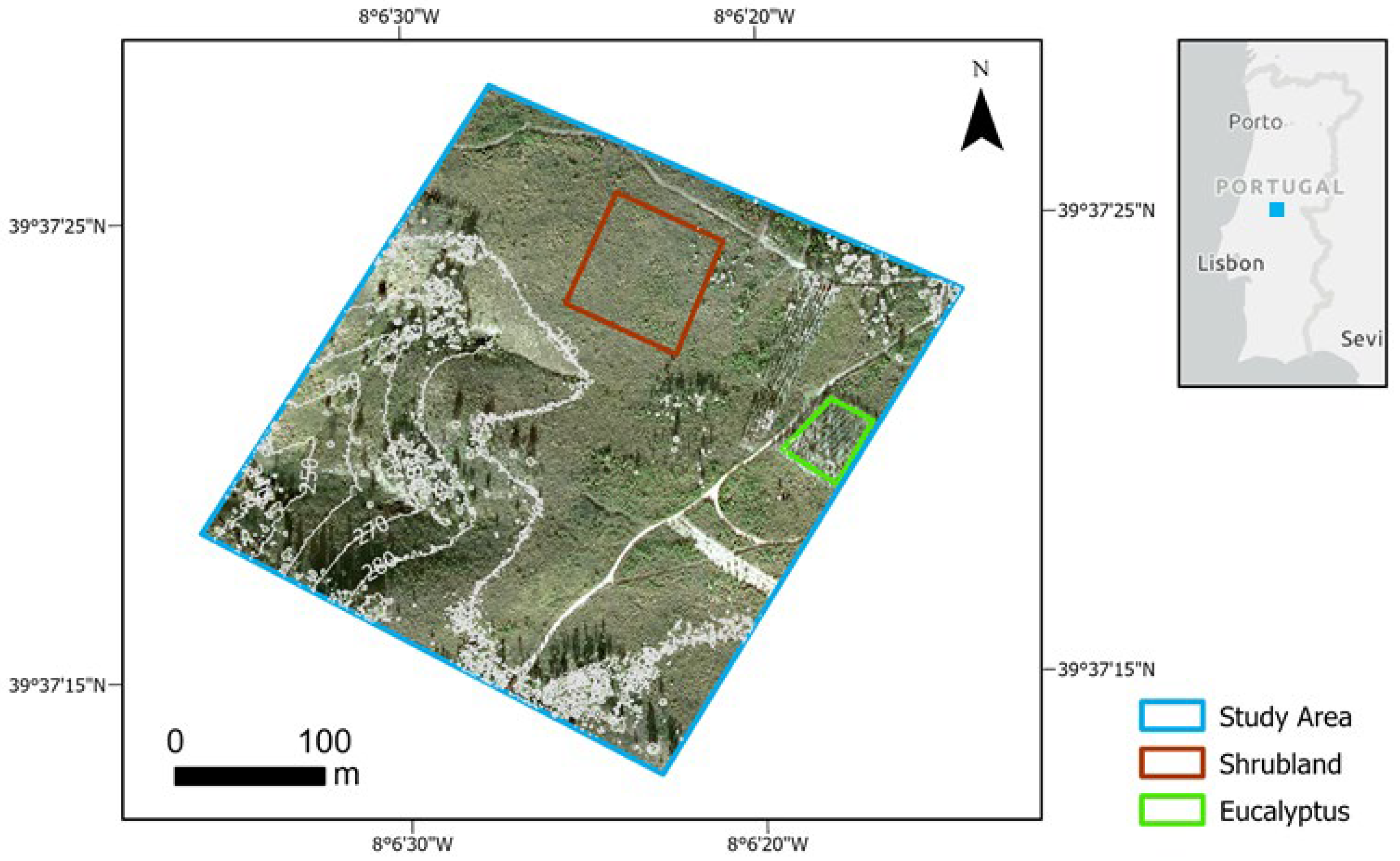
The study area is located 8 km to the southwest of the geodetic center of Portugal (around 39°37′20″ N 8°6′25″ W, Figure 2), in a Mediterranean climate zone at the transition of Köppen-Geiger classes Csa and Csb, with dry summers and an average temperature of 22 °C in the warmest month [12]. It is a plateau of sedimentary sandstone deposits, at an elevation of 240–250 m above sea level. A wildfire affected the study area on 13 August 2017 [13], and the fire severity varied between moderate and high [14]. Before the wildfire, the tree coverage was approximately 90% Maritime Pine (Pinus pinaster Ait.) and 10% Eucalypt (Eucalyptus globulus Labill.). All pine trees were killed by the fire, and all the shrubs were consumed, making it impossible to determine which shrub species were present. The dominant shrub species when this study was done (2022–2024) were Arbutus unedo, Cistus psilosepalus, Agrostis truncatula, and Cistus ladanifer, and the tree species Pinus pinaster and Eucalyptus globulus. The study area covers 128,763 m2. Within the study area, two sub-areas were selected to determine cover-related influences in the results: the ‘Shrubland’ sub-area, with 6610 m2, corresponding to the shrubs; and an ‘Eucalyptus’ sub-area, with 1774 m2, corresponding to an area where the soil was ploughed, and Eucalyptus were planted in early spring of 2021.

2.3. Data Acquisition

2.3.1. UAS Data Acquisition

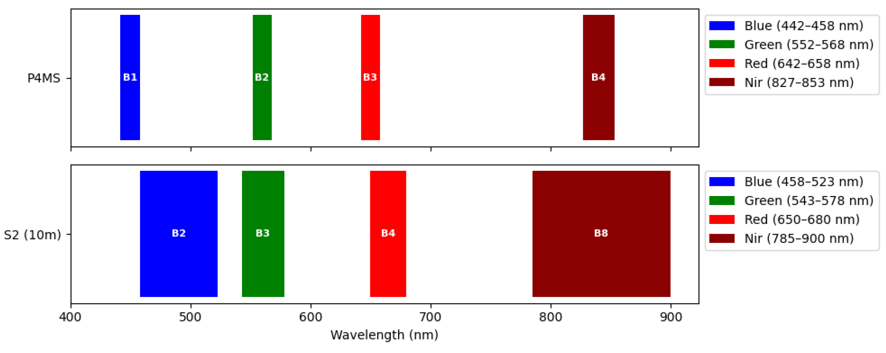
UAS data acquisition was carried out with the DJI Phantom 4 Multispectral RTK (P4MS) (DJI, Shenzhen, China) equipped with a real-time kinetics (RTK) module, a 5-band multispectral camera, and an incident light sensor (ILS). The multispectral setup of P4MS includes a red band (B3) centered at 650 nm (with 16 nm bandwidth) and a Near-Infrared (NIR) band centered at 840 nm (with 26 nm bandwidth), both being relevant for NDVI calculation (Figure 3). To ensure accurate and reliable data, RTK was always enabled, and ground control points (GCPs) were deployed and fixed in the area to improve and validate the geometric accuracy. The GCPs were georeferenced with a Trimble R780 (Trimble Inc., Sunnyvale, CA, USA) Global Navigation Satellite System (GNSS) receiver in RTK mode. One Spectralon reflectance panel (Labsphere, North Sutton, NH, USA) was set up on each flight day to radiometrically correct the images during the data processing phase. To minimize shadows, UAS flights took place at solar noon. This coincided with the Sentinel-2 overpass window (between 11:00 and 12:00 UTC), maintaining consistency across both data sources. The flight missions were planned and executed with the DJI GS Pro app for iOS. The flown area covers the same as the study area, the ground sampling distance (GSD) was set to 0.04 m/pixel, and the front and side picture overlap was set to 75%. The app automatically adjusts the flight lines’ angle throughout the year to align the ILS sensor perpendicularly with the solar radiation. More details can be found in [15]. In total, the data from fourteen flights were included in this study (Table 1).

2.3.2. Sentinel-2

The Sentinel-2 (S2) mission operates as a constellation of identical satellites, which for the study period included Sentinel-2A (S2A) and Sentinel-2B (S2B) [16]. Both satellites include a Multispectral Instrument (MSI), including visible and NIR region bands with a spatial resolution up to 10 m. Those bands relevant for calculating the NDVI at such spatial resolution include the red band (B4), which is centered at 665 nm (with a 30 nm bandwidth), while the NIR band (B8) is centered at 842 nm (with a 115 nm bandwidth) [16] (Figure 3).
To enable multitemporal and spatial analysis, S2 Level 2A Surface Reflectance products provide radiometric, geometric, and atmospheric corrections, ensuring S2A and S2B consistency [16].
The analysis and processing of long time series of S2 data is often a highly time-consuming and computationally intensive task due to the frequent satellite revisit times. The Google Earth Engine (GEE) platform, with its big data processing capabilities [17] is particularly useful in such tasks. At the moment of writing of this article, the GEE Data Catalogue includes two S2 Surface Reflectance product series: Non-Harmonized (S2_SR) and Harmonized (S2_SR_HARMONIZED).
The S2 Harmonized dataset was developed in response to the changes implemented with PROCESSING_BASELINE ‘04.00’ (from 25 January 2022), which introduced a radiometric offset at Level-1C (and propagated to Level-2A) to preserve negative values over dark surfaces—preventing information loss due to clamping [18]. In practice, Non-Harmonized products with a PROCESSING_BASELINE ‘04.00’ or above have their DN (value) range shifted by +1000. The Harmonized collection shifts newer scenes to match older (i.e., pre-‘04.00’) ranges for temporal consistency across processing baselines. In both cases, the S2A/S2B inter-sensor consistency is maintained via L2A processing.
In this study, both the S2 Non-Harmonized and Harmonized series were included to provide a comprehensive analysis of the potential effects of radiometric processing and harmonization on NDVI retrievals. The Non-Harmonized series represents the original Level-2A Surface Reflectance products directly provided by the Copernicus program. In contrast, the Harmonized series is a derivative dataset provided through Google Earth Engine, designed to adjust for radiometric inconsistencies introduced with PROCESSING_BASELINE ’04.00’ and later. While the Harmonized dataset improves comparability between older and newer scenes, it may also introduce subtle biases or artifacts. Direct comparisons between harmonized and non-harmonized Sentinel-2 time series remain scarce in the literature. Including both series allows for a more robust assessment of S2 data reliability and facilitates understanding of the potential implications of radiometric harmonization when comparing satellite and UAS-derived vegetation indices.
Using the GEE platform, every available scene with up to 15% overall cloud cover was considered in order to extract the corresponding bands 4 (RED) and 8 (NIR) and directly calculate the NDVI values of each scene and export to geoTIFF format. After implementing the GEE script, a total of 30 images were selected from each S2 Harmonized and Non-Harmonized series.

2.4. Data Processing and Analysis

The P4MS images were processed with Agisoft Metashape Professional version 2.1 (Agisoft LLC, St. Petersburg, Russia). Image processing followed the guidelines given by [15]. Software parameters for picture alignment were set to high, followed by a bundle block adjustment using one GCP, which, together with RTK, is expected to ensure a geometric accuracy in the order of about 5 cm or better. The radiometric correction was executed with laboratory reflectance values from a reflectance panel introduced in the area flown on each acquisition mission. ILS data was included for overcast days.
The multispectral band setup of P4MS and S2 sensors (Figure 3) provides a solid basis for using vegetation indices. This alignment further justifies the use of the NDVI, which maximizes the contrast between the strong reflectance of healthy vegetation and its absorption in the RED, being particularly relevant for differentiating vegetation and soil, even under variable reflectance conditions. One key difference between UAS and satellite remote sensing datasets is spatial resolution. P4MS orthophotomaps and corresponding NDVI were generated at 0.04 m spatial resolution, while the S2 and corresponding NDVI maps have a 10 m spatial resolution. To match both datasets in terms of pixel size, the ArcGIS Pro software version 3.6.1 (Esri, Redlands, CA, USA) includes two main groups of raster rescaling methods: the Aggregate (Spatial Analyst) and the Resample (Data Management) tools [19]. The Aggregate Mean function was selected for rescaling P4MS data from 0.04 m to 10 m resolution because it provides the most appropriate statistical representation of spectral values within each aggregated pixel, preserving critical vegetation index characteristics while minimizing methodological bias. The use of aggregate mean conserves the bulk signal while filtering out small-scale noise. Unlike interpolation-based resampling methods such as nearest neighbor, bilinear, or cubic convolution, which are designed for geometric transformation rather than statistical summarization, the aggregate mean function performs spatial aggregation towards a coarser resolution by calculating the arithmetic average of all high-resolution pixels contained within each target grid cell, ensuring that no spectral information is artificially created or lost. The aggregate mean was calculated with snapping in respect to one S2 MSI scene (for pixel alignment purposes).

3. Results

3.1. Temporal Analysis

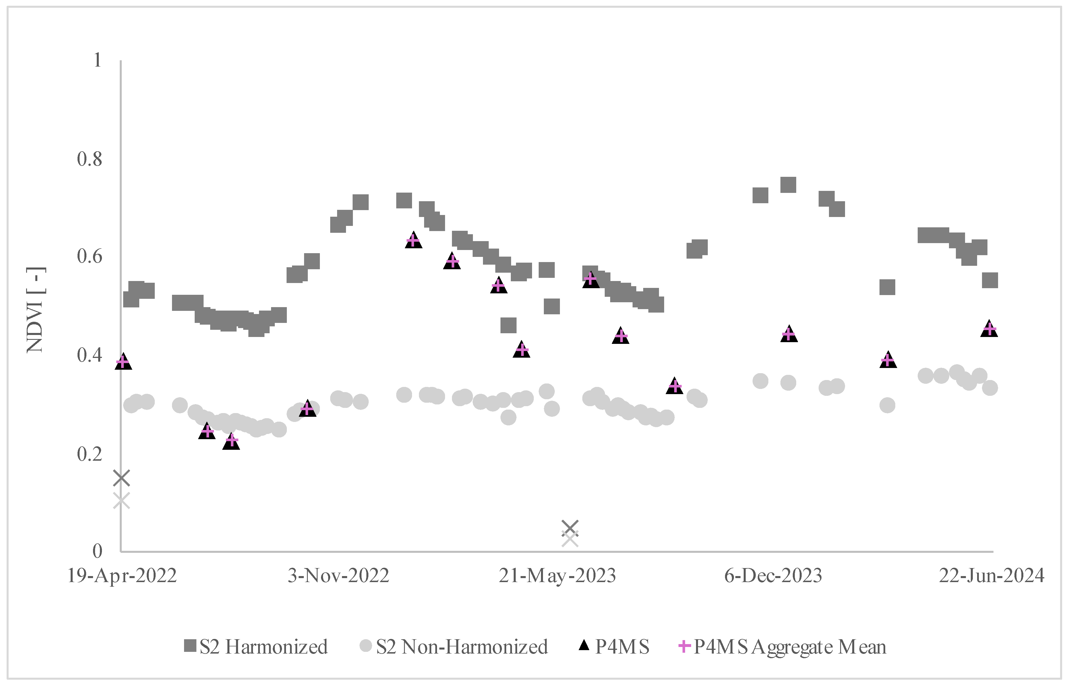
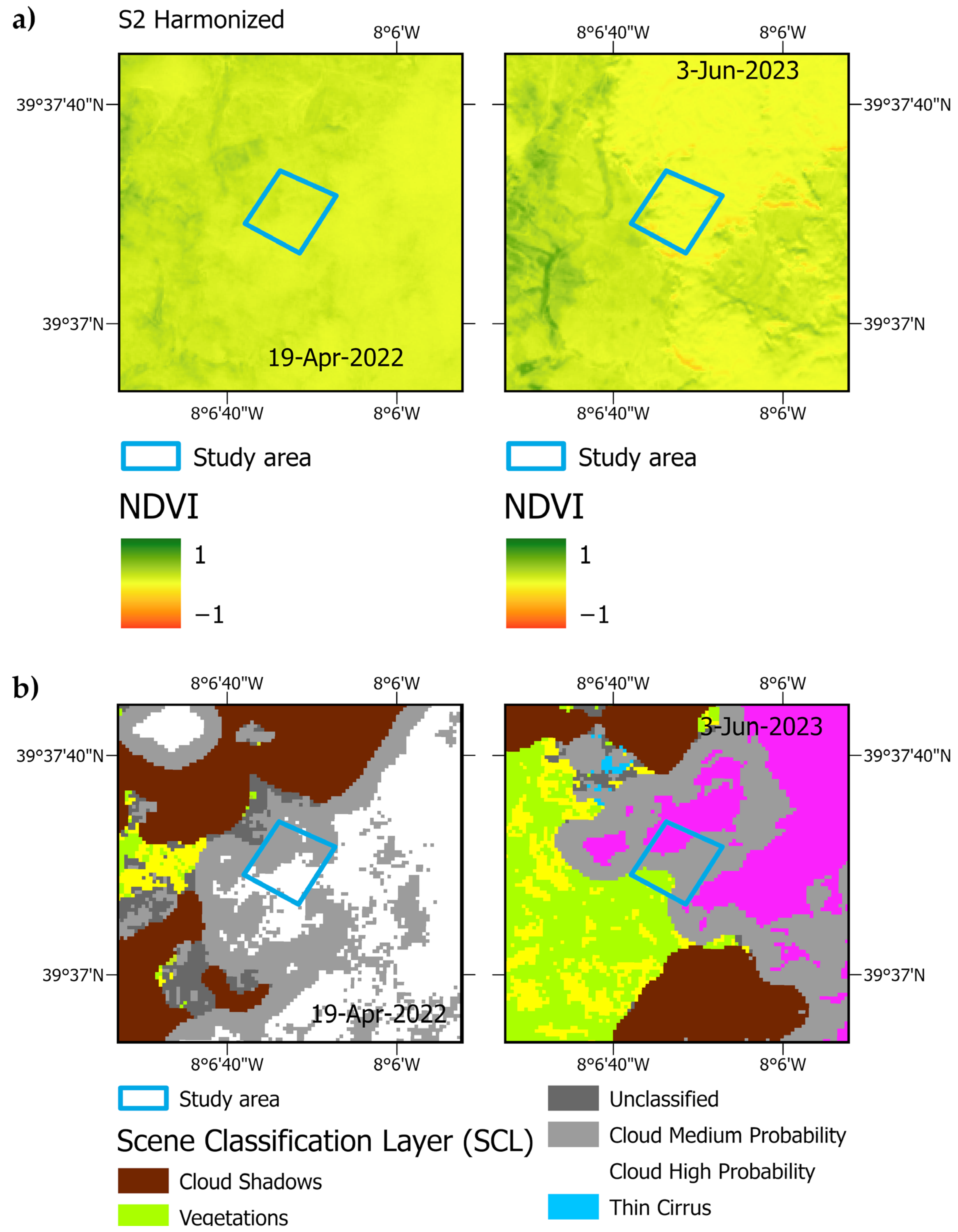
Figure 4 includes an overview of the time series of each platform, as mean NDVI values, obtained from S2 MSI Harmonized and Non-Harmonized datasets (10 m pixel size), alongside the P4MS datasets (0.04 m pixel size and 10 m aggregate pixels) for the entire study area. Despite only including scenes with overall cloud coverage under 15%, both S2 series include two significantly lower values of NDVI on 19-Apr-2022 and 3-Jun-2023. A visual inspection of the NDVI maps for these scenes (Figure 5) revealed that the study area was heavily affected by clouds/cloud shadows on those dates. This was confirmed by the occurrence of minimal NDVI values and the Scene Classification Layer (SCL) included with S2 Level-2A products, which identified such pixels as medium/high cloud probability, or snow (the latter likely corresponding to a false detection of high-altitude clouds, as suggested by [20]. For this reason, these scenes were discarded from further analysis.
For all datasets, the time series demonstrates the fundamental seasonal rhythms characteristic of vegetation phenology, with pronounced variations in NDVI values corresponding to different growth stages and environmental conditions. For the studied period, the mean NDVI of the S2 Harmonized series ranged from 0.45 to 0.74, and the S2 Non-Harmonized series ranged from 0.24 to 0.36 (Figure 4), highlighting the impact of different baseline processing methodologies.
A comparison of the two S2 time series reveals consistent seasonal variations, with the harmonized series showing higher annual amplitude than the Non-Harmonized. Both S2 series have higher mean NDVI values in winter scenes, and the highest difference (54%) between Harmonized and Non-Harmonized was observed on 20-Dec-2023. The S2 Harmonized series consistently provides higher NDVI values throughout the time series, with the difference between Harmonized and Non-Harmonized more pronounced during peak growing seasons. This effect is a consequence of the radiometric offset between both dataset series. The initial 1000 DN offset, when transformed into NDVI, introduces −2000 in the Harmonized series denominator, which increases the NDVI values.
The overlapping symbols demonstrate that the ArcGIS aggregate mean function used to transform the 0.04 m P4MS data (black triangles in Figure 4) to 10 m resolution (purple crosses in Figure 4) preserves the mean NDVI values, an arithmetic consequence of the mean of the aggregated means equalling the mean of all 4 cm P4MS values, since each aggregation contains the same number of observations. For this reason, within the study area, the spatial heterogeneity at sub-10 m scales does not affect the aggregated mean NDVI value.
The overall amplitude of mean P4MS values demonstrates greater variation than either of the S2 series, ranging from 0.22 to 0.63. This enhanced dynamic range reflects the higher spatial resolution and sensor sensitivity of the drone-based platform. The highest mean NDVI values in the P4MS data were registered in winter, with summer/early autumn resulting in the lowest values, following a similar seasonal pattern to the satellite data but with greater amplitude variation.
In comparison to the closest coeval S2 scenes, the lower mean P4MS values (NDVI = 0.41) are closer to the Non-Harmonized series (|bias| = 0.06 vs. 0.19), while higher values are closer to the Harmonized series (|bias| = 0.06 vs. 0.23).
While the four data series capture the fundamental seasonal dynamics (Figure 4), differences emerge in spatial expression across scales and processing variants, justifying an in-depth spatial analysis.

3.2. Spatial Analysis

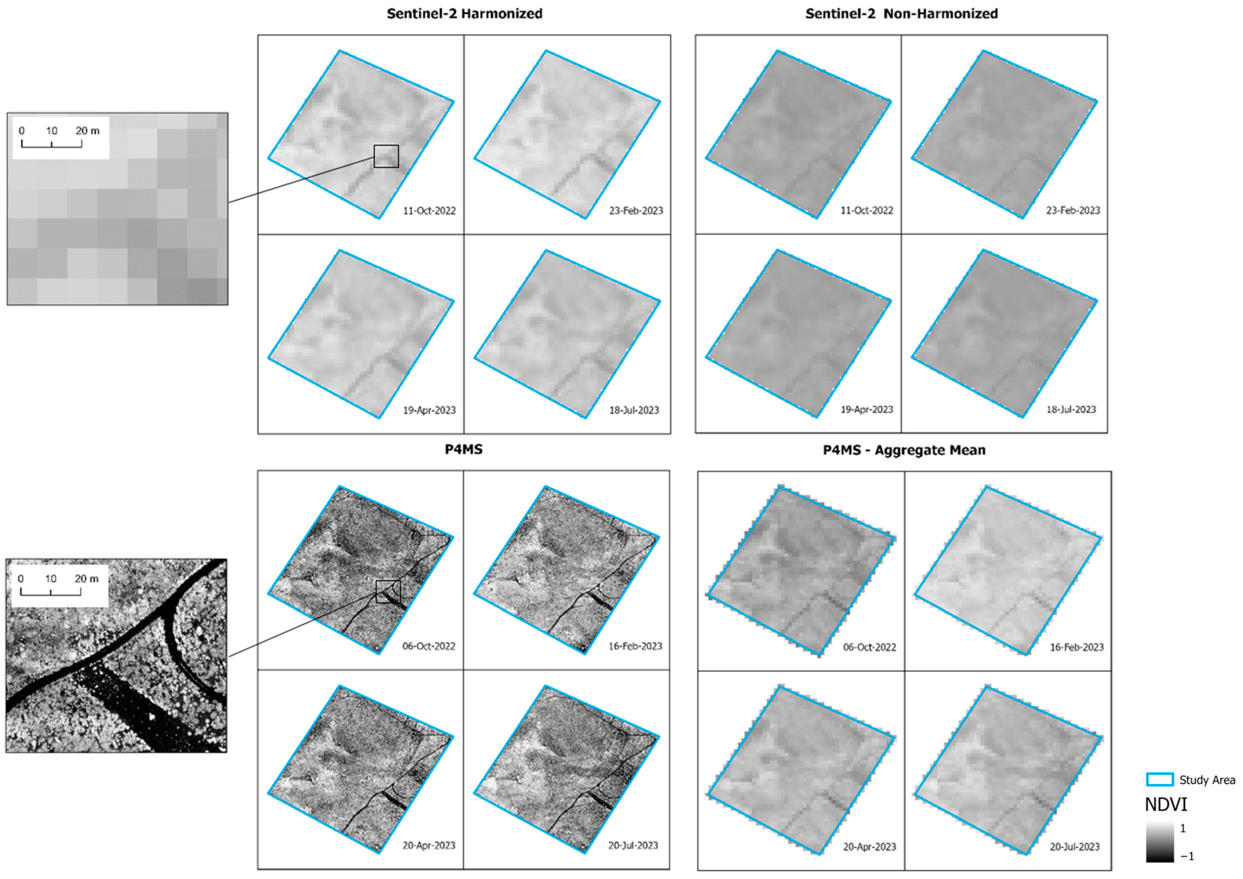
In order to do a detailed pixel-by-pixel spatial analysis, four dates were selected for representing four consecutive seasons: 11-Oct-2022 (autumn), 23-Feb-2023 (winter), 19-Apr-2023 (spring), and 18-July-2023 (summer). The selection of these dates was based on the temporal proximity between satellite overpass and UAS flight, i.e., the closest coeval scenes were chosen. Figure 6 presents the NDVI values of each 10 m pixel for the datasets S2 Harmonized, S2 Non-Harmonized, P4MS Aggregate Mean, and 0.04 m pixel for the P4MS dataset. The figure also shows insets, both depicting the same location—which features a pathway intersection and a young eucalyptus plantation—but at different spatial resolutions.
The S2 Harmonized and Non-Harmonized NDVI maps consistently display broad-scale gradients in greenness aligned with vegetation patterns observed in the field. However, the Harmonized maps, across all four scenes examined, visibly exhibit slightly higher brightness and spatial contrast, corresponding to elevated NDVI values as previously demonstrated in the temporal analysis. As a consequence of the NDVI transformation, the differences between both S2 series become no longer a simple additive offset, manifesting as a non-linear rescaling of NDVI values that compensates for the compression of Non-Harmonized data and restores its dynamic range; such transformation enhances subtle spatial texture and the demarcation of medium- and high-NDVI zones. This increased NDVI contrast is especially conspicuous during winter and spring dates (23-Feb-2023, 19-Apr-2023), underscoring the influence of the radiometric offset correction applied during harmonization on the preservation of phenological gradients and intra-field spatial heterogeneity. In comparison, the S2 Non-Harmonized NDVI maps appear dimmer and less spatially contrasted, reflecting the compression of NDVI values caused by the DN offset in Processing Baseline ≥ ‘04.00’. Patches that are silhouetted clearly in the Harmonized product become more diffuse and homogeneous in the S2 Non-Harmonized version, particularly during phases of maximum vegetative vigor. When inspected visually at a given spatial resolution and bit depth, this apparent dampening of contrast may complicate the discrimination of vegetation states or subtle management effects at the landscape scale when using Non-Harmonized data and NDVI, especially for applications requiring multi-temporal spatial change detection.
The original 0.04 m P4MS scenes reveal fine-scale details—including individual tree crowns and narrow tracks—and display the widest NDVI range of all datasets, as would be expected with the higher resolution. These details, which are spatially aliased in S2 products, highlight the advantage of UAS multispectral mapping for applications requiring the discrimination of small-scale ecological processes. After aggregation to 10 m, the P4MS scenes maintain their overall mean NDVI values while smoothing extreme highs and lows, with key structural patterns and contrast between vegetated and non-vegetated areas remaining visible.
Spatial patterns observed across the four dates reveal the dynamic response of vegetation to seasonal change (in agreement with Figure 4), visible at both 10 m and 0.04 m resolutions. During autumn and winter, all four datasets show relatively elevated NDVI levels, with the most vigorous zones delineated clearly. In spring, a slightly patchier spatial structure emerges, possibly linked to phenological lags or small-scale soil moisture effects. By summer, NDVI intensity is somewhat diminished, and spatial heterogeneity increases, as evidenced by a broader spectrum of patch sizes and contrasts within the P4MS and, to a lesser extent, in the P4MS aggregate mean and S2 maps. The synchronous nature of these spatial trends across platforms supports the conclusion that inter-annual and intra-annual variation in vegetation condition is reliably reflected in all datasets. Still, only the P4MS 0.04 m resolution product exposes the finer grain of these changes, revealing the within-field variability concealed at the satellite scale. Seasonal contrasts in the prominence of these patterns underscore how temporally dynamic processes manifest spatially at scales ranging from meters to tens of meters.
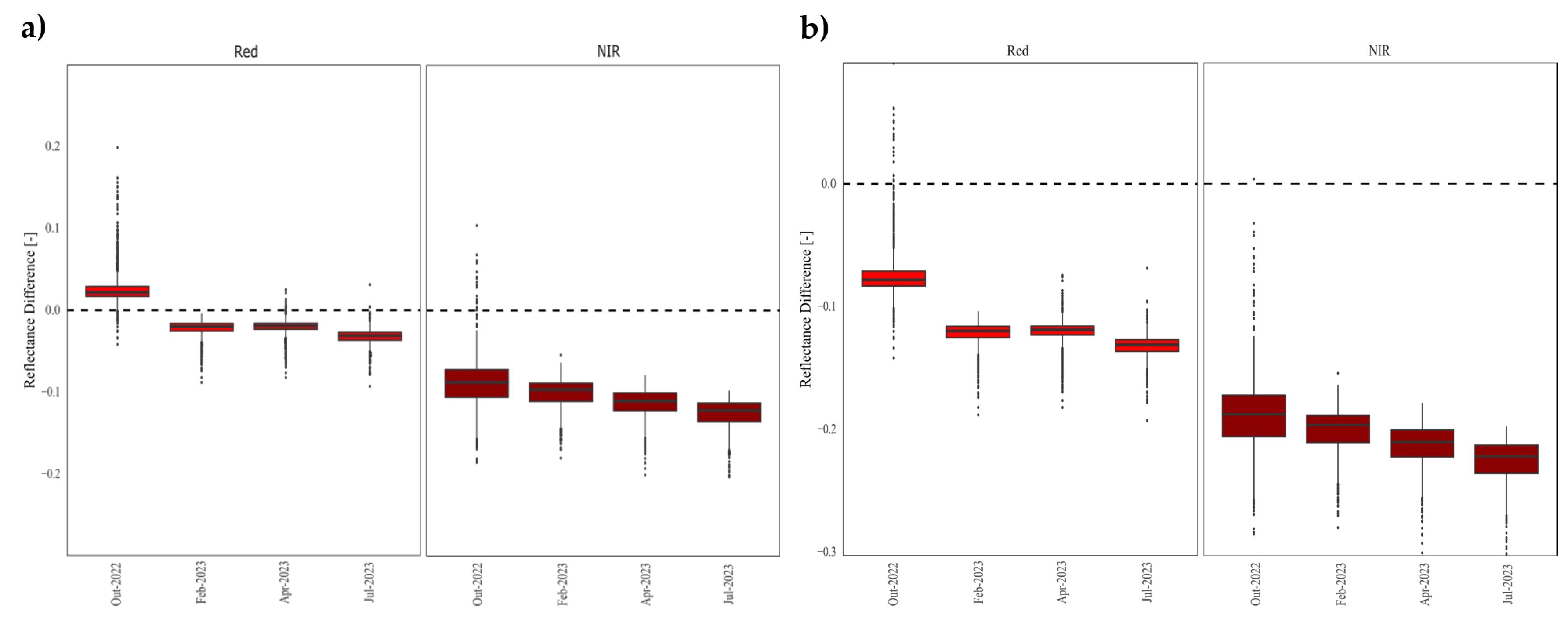
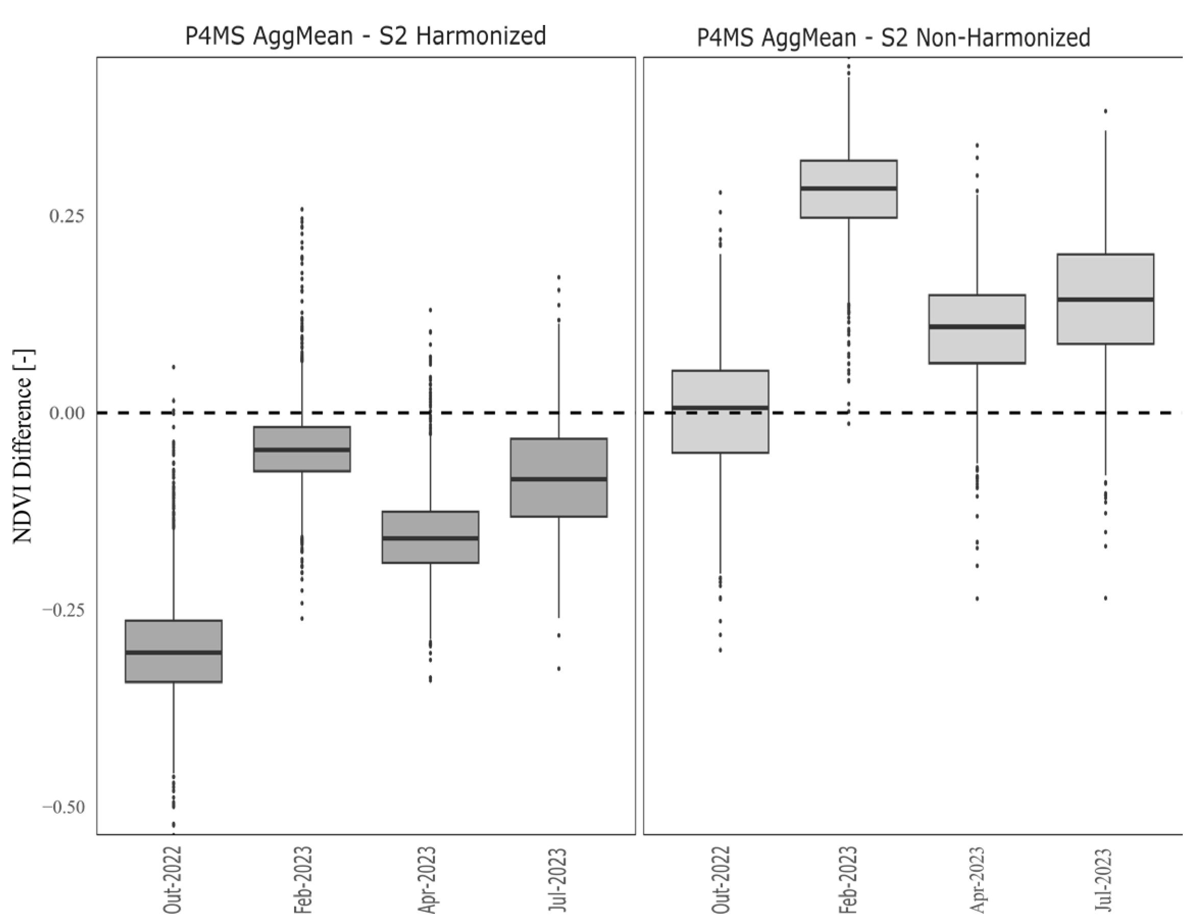
To understand the impact of radiometric harmonization on cross-platform data integration and, ultimately, on vegetation monitoring accuracy, we analyzed spatial variability in reflectance differences using boxplots (Figure 7). Figure 7a,b show the differences between the rescaled P4MS and S2 MSI Harmonized and S2 MSI Non-Harmonized series, respectively, for the RED and NIR bands across the same four seasonal scenes from October 2022 to July 2023. Each boxplot represents n = 1278 10-m pixels, providing robust statistical representation of the spatial distribution of sensor differences across the study area. The temporal analysis suggests a systematic drift in sensor relationships over this study period. The increasingly negative trend suggests that the P4MS sensor consistently measures lower reflectance values compared to the S2 MSI sensor as time progresses from October 2022 to July 2023. This temporal drift pattern is particularly pronounced in the NIR band, where the spatial variability also increases substantially over the same period.
For the Non-Harmonized series (Figure 7b), differences are consistently negative in all scenes, indicating a systematic underestimation of reflectance values compared to the rescaled P4MS data throughout the entire study period. In contrast, the Harmonized series (Figure 7a) shows a positive difference in the RED band for the October 2022 scene, while exhibiting negative differences in both bands for the remaining dates. A comparison between Figure 7a,b reveals that the offset is more substantial relative to the S2 Non-Harmonized series than to the S2 Harmonized series, especially in autumn and winter scenes. This pattern suggests that radiometric harmonization of S2 translates to greater consistency and reduced overall bias in the comparison with high-resolution UAS reflectance data.
The consistent spatial patterns observed across all seasonal scenes demonstrate that the temporal drift is spatially uniform across the study area. The boxplot statistics show that while individual pixel-level variations exist, the overall temporal trend is systematic and affects the entire spatial domain similarly. The persistence of outlier patterns across temporal scenes suggests a consistent spatial heterogeneity in sensor responses, with specific locations showing extreme differences that remain spatially consistent over time. This spatial persistence suggests site-specific factors such as topographic effects, vegetation structure, or soil background that consistently influence sensor comparisons.
Evaluation of Figure 7a,b underscores the critical role of S2 data harmonization for multi-sensor research. Across both bands and all seasons, reflectance differences relative to the Harmonized series are consistently less negative, have narrower interquartile and whisker ranges, and have fewer extreme outliers compared to differences relative to the Non-Harmonized series.
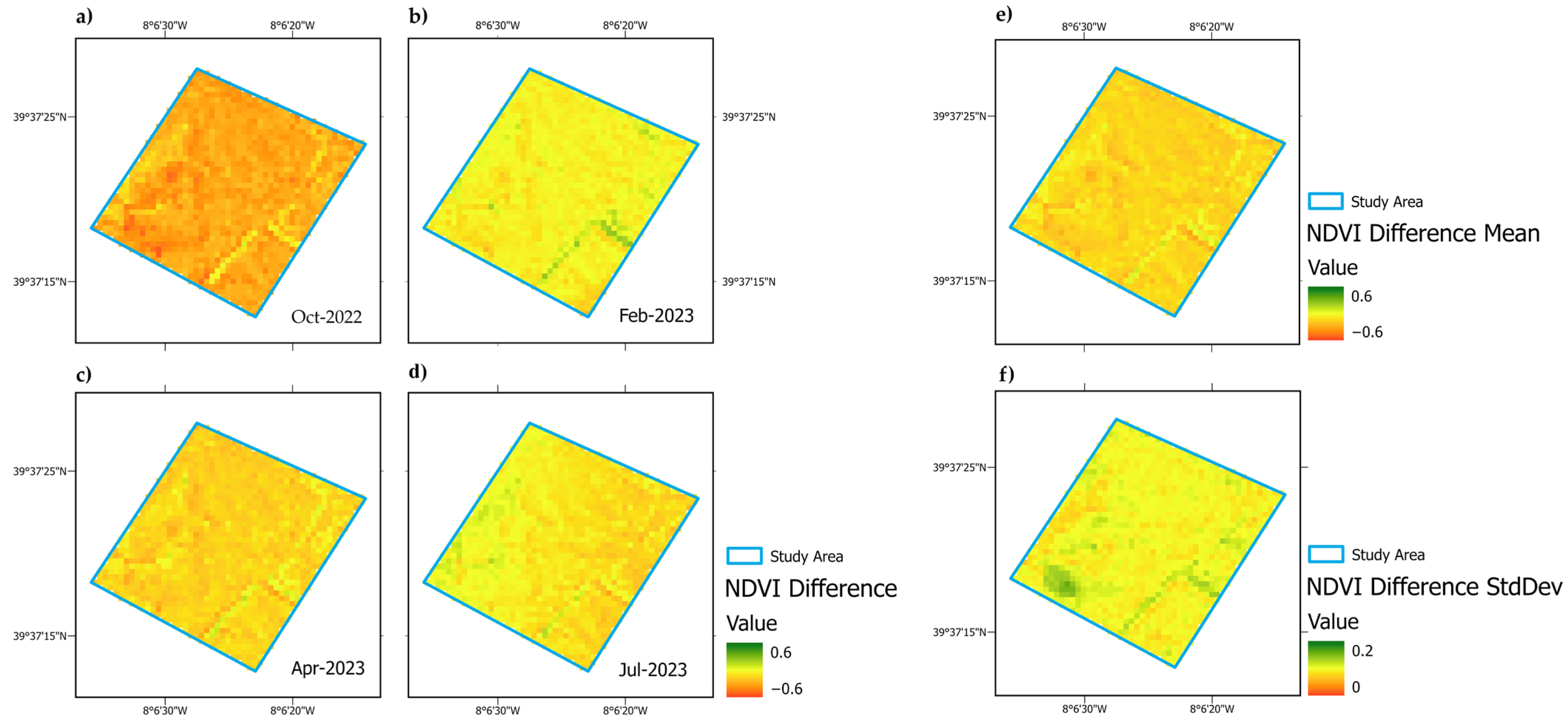
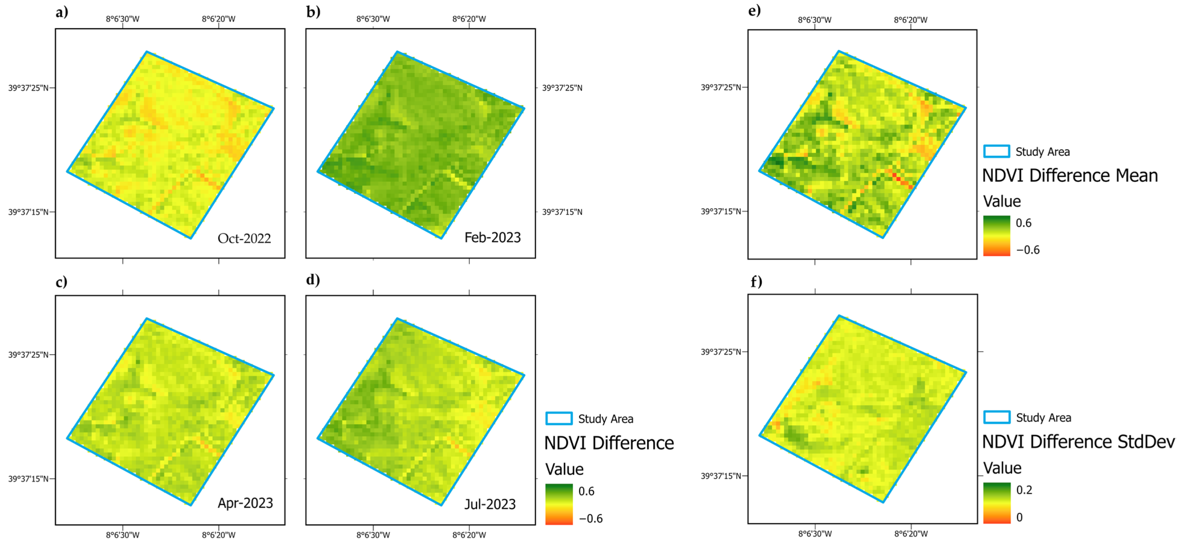
Figure 8 and Figure 9 present comprehensive NDVI difference maps calculated as P4MS Aggregate Mean minus S2 Harmonized and Non-Harmonized datasets (n = 1278 10-m pixels per map), respectively, across four seasonal examples and summary statistics spanning the entire time series (n = 12 scenes). These maps (together in the boxplots in the Appendix A, Figure A1) reveal distinct patterns in sensor agreement that vary both temporally and spatially.
For the autumn scene, Figure 8 illustrates a predominantly orange tint, indicating that P4MS Aggregate NDVI Mean values are consistently lower than S2 Harmonized observations. The observed difference ranges from –0.54 to +0.05 NDVI units, and minority green flecks cover less than 1% of the area, reflecting only rare cases where P4MS exceeds S2 Harmonized. In contrast, Figure 9 (autumn) displays a lighter orange-to-yellow palette, demonstrating smaller negative differences between P4MS Aggregate Mean and S2 Non-Harmonized, ranging from −0.30 to +0.27 NDVI units, with some small green patches indicating a few locations where P4MS is higher. The winter scene (February 2023) notably shifts for both products. Figure 8 transitions to a more yellow-green pattern in several areas, signaling that the difference between the P4MS Aggregate Mean and S2 Harmonized approaches is zero or mildly positive, with values from −0.26 up to +0.26 NDVI. This patchiness reflects partial seasonal convergence in NDVI readings. Figure 9, however, is considerably more green, showing the largest areas with positive (P4MS > S2 Non-Harmonized) differences, which can exceed +0.50 NDVI in parts of the study area. This indicates instances where the P4MS Aggregate NDVI Mean reads higher NDVI than the S2 Non-Harmonized, most prominently in winter. Spring (April 2023) in Figure 8 presents a predominantly yellow pattern, with some light green and orange patchiness, meaning differences are close to zero or mildly negative—ranging between −0.33 and 0.13—though some localized patches differ more strongly. Figure 9 continues this green pattern, suggesting P4MS readings are frequently higher than S2 Non-Harmonized throughout the scene in spring as well. During summer (July 2023), Figure 8 displays a mostly uniform light-orange tone, with mean differences of −0.08 NDVI across the study area and relatively little variance. Figure 9 is more yellow-green in summer, again indicating that P4MS Aggregate Mean is closer or even higher than S2 Non-Harmonized NDVI in many areas.
Panel (e) in both figures shows the long-term mean of these differences, and panel (f) shows the standard deviation across scenes. In Figure 8e (Harmonized), the mean difference map is a blend of yellow and orange, with the majority of the area having a negative mean difference but some local green indicating zones where P4MS can surpass S2 Harmonized on occasion. In Figure 9e (Non-Harmonized), the mean difference is more spatially heterogeneous, with frequent yellow-green patches, indicating a more balanced difference between P4MS and S2 Non-Harmonized over time. Standard deviation panels (f) from both figures (especially Figure 8f) highlight slightly higher variability in certain regions, albeit with overall low to moderate interannual variation. Appendix A, Figure A1 boxplots confirm these visual trends: the P4MS Aggregate Mean consistently reads lower NDVI than S2 Harmonized (median differences mostly negative across all seasons), while the comparison with S2 Non-Harmonized is more variable and includes more instances of positive difference, especially in winter and spring. The interquartile ranges of the boxplots are in line with the spatial variability seen in the maps.
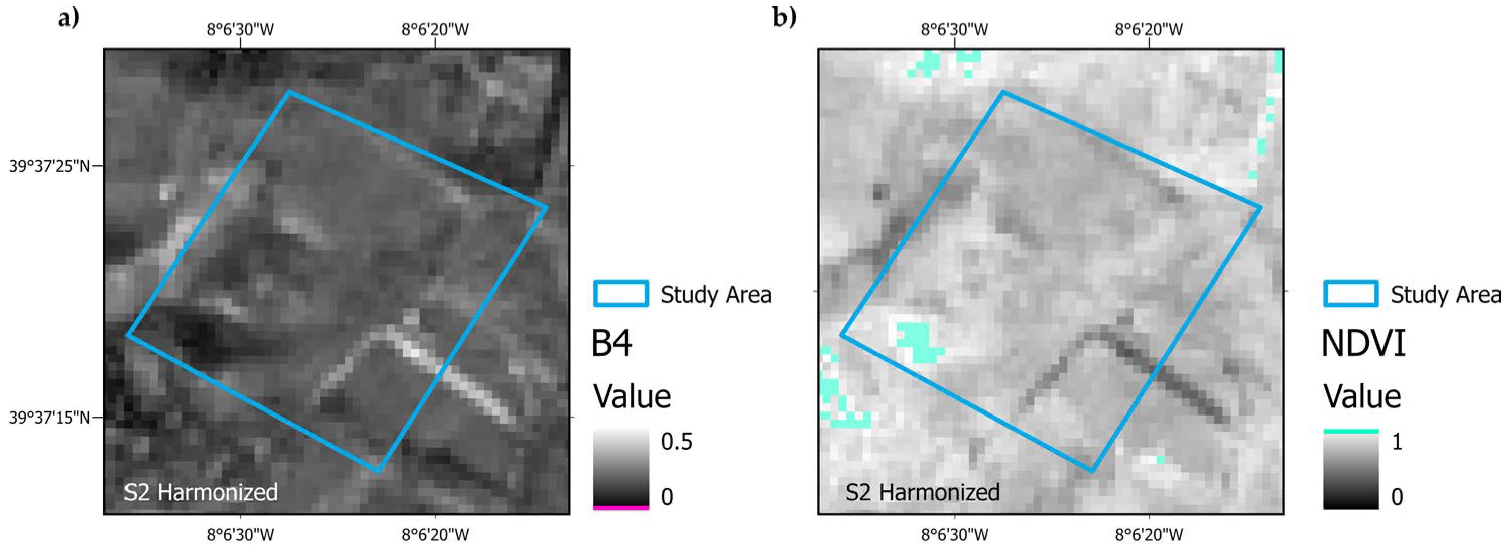
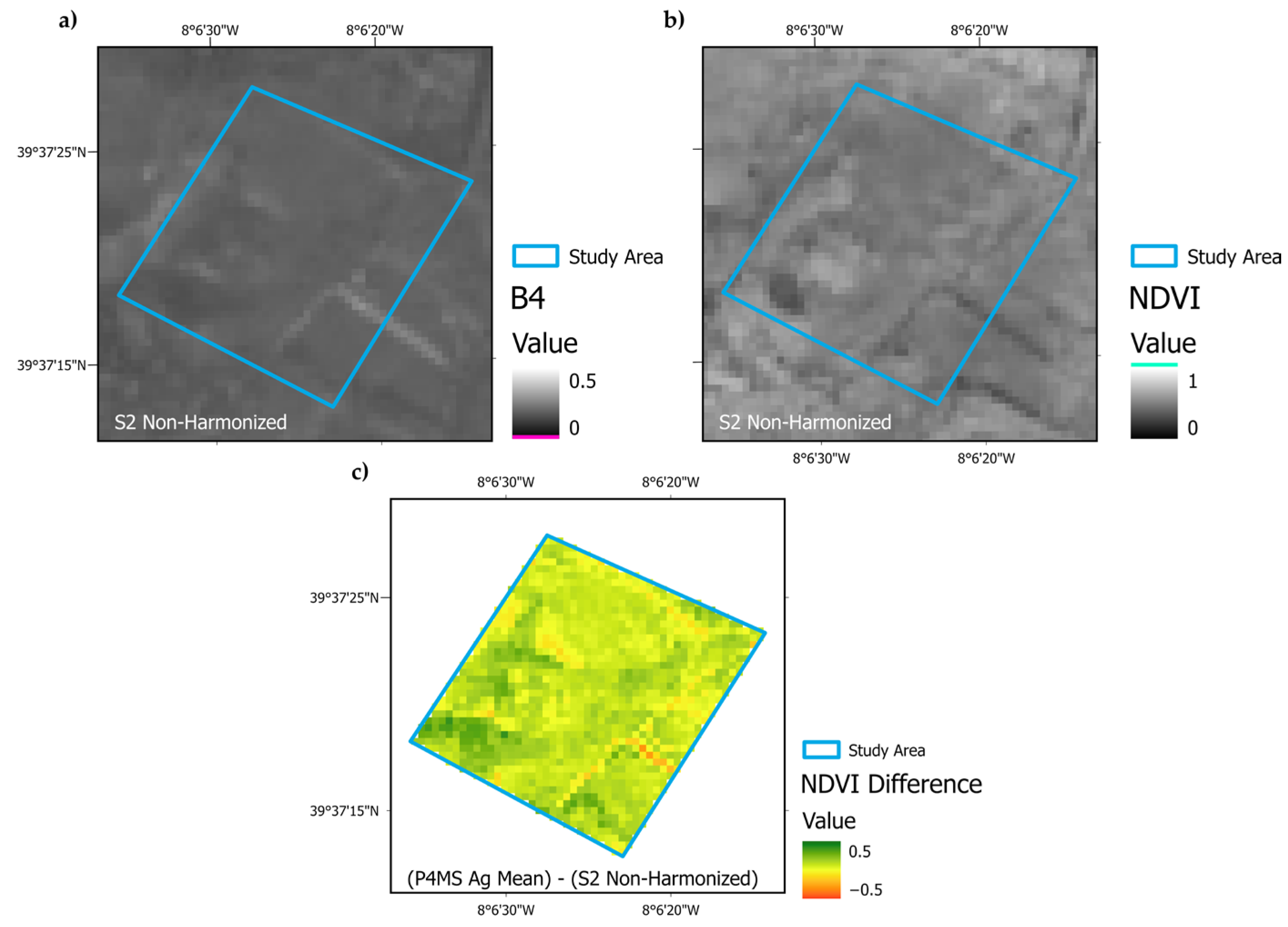
To better understand some of the apparent spatiotemporal differences between both S2 series, an additional analysis was conducted for the 20-Dec-2023 scene (Figure 10), focusing on the RED band (B4) and NDVI values derived from the S2 Harmonized dataset. This analysis reveals that for the Harmonized series, the RED band contains several areas with reflectance equal to 0 (Figure 10a, in purple), which in turn leads to NDVI values equal to 1 (Figure 10b, in cyan) because the NIR reflectance in these pixels is non-zero. These NDVI = 1 values are artifacts resulting from zero RED reflectance and are absent in the corresponding Non-Harmonized series (Appendix A, Figure A1). A comparison with the original high-resolution orthophotomap (Figure 2) confirms that these areas correspond to shadowed locations, caused by local topography—due to lower elevations and northwest-facing slopes.
The statistical analysis of NDVI differences between P4MS Aggregate NDVI Mean and S2 (Table 2) reveals fundamental disparities between Harmonized and Non-Harmonized processing approaches across the four seasonal scenes examined. The dataset encompasses 1278 10-m pixels per comparison, providing robust statistical power for detecting systematic biases and distributional characteristics.
When comparing P4MS Aggregate NDVI Mean to S2 Harmonized NDVI, all seasonal periods demonstrate consistently negative mean differences, ranging from −0.297 in October 2022 to −0.043 in February 2023. The median difference values closely mirror the means, with differences typically within 0.01 NDVI units, indicating relatively symmetric distributions. October 2022 exhibits the most pronounced negative bias with a mean difference of −0.297 and a median of −0.304, suggesting that P4MS values are systematically lower than S2 Harmonized NDVI values during autumn conditions. February 2023 shows the smallest bias magnitude with a mean difference of −0.043 and a median of −0.047, indicating improved agreement during winter conditions. In contrast, the comparison between P4MS Aggregate Mean and S2 Non-Harmonized data reveals predominantly positive differences across all seasons. October 2022 shows near-zero bias with a mean difference of 0.002 and a median of 0.006, representing the closest agreement between sensor systems. February 2023 exhibits the largest positive bias with a mean difference of 0.281 and a median of 0.285, indicating that P4MS values substantially exceed S2 Non-Harmonized observations during winter conditions. Spring and summer periods maintain moderate positive biases, with mean differences of 0.105 and 0.144, respectively. The shape and symmetry of NDVI difference distributions further illuminate these seasonal patterns. Harmonized comparisons are right-skewed in all seasons, meaning most pixels show negative differences but a minority reach near-zero or positive values; their heavy tails (kurtosis) underscore occasional large outliers. Non-Harmonized comparisons tend toward a slight left skew in most seasons, reflecting a predominance of positive differences with some pixels showing lower or negative offsets, and exhibit more moderate kurtosis. These distributional characteristics signal that simple mean corrections will not fully address the complex bias and tail behavior inherent in multi-sensor datasets. Temporally, the magnitude and sign of mean NDVI differences follow distinct seasonal rhythms depending on processing: S2 Harmonized bias decreases steadily from pronounced autumn underestimation to minimal winter offset, whereas S2 Non-Harmonized bias peaks in winter before subsiding through spring and summer.
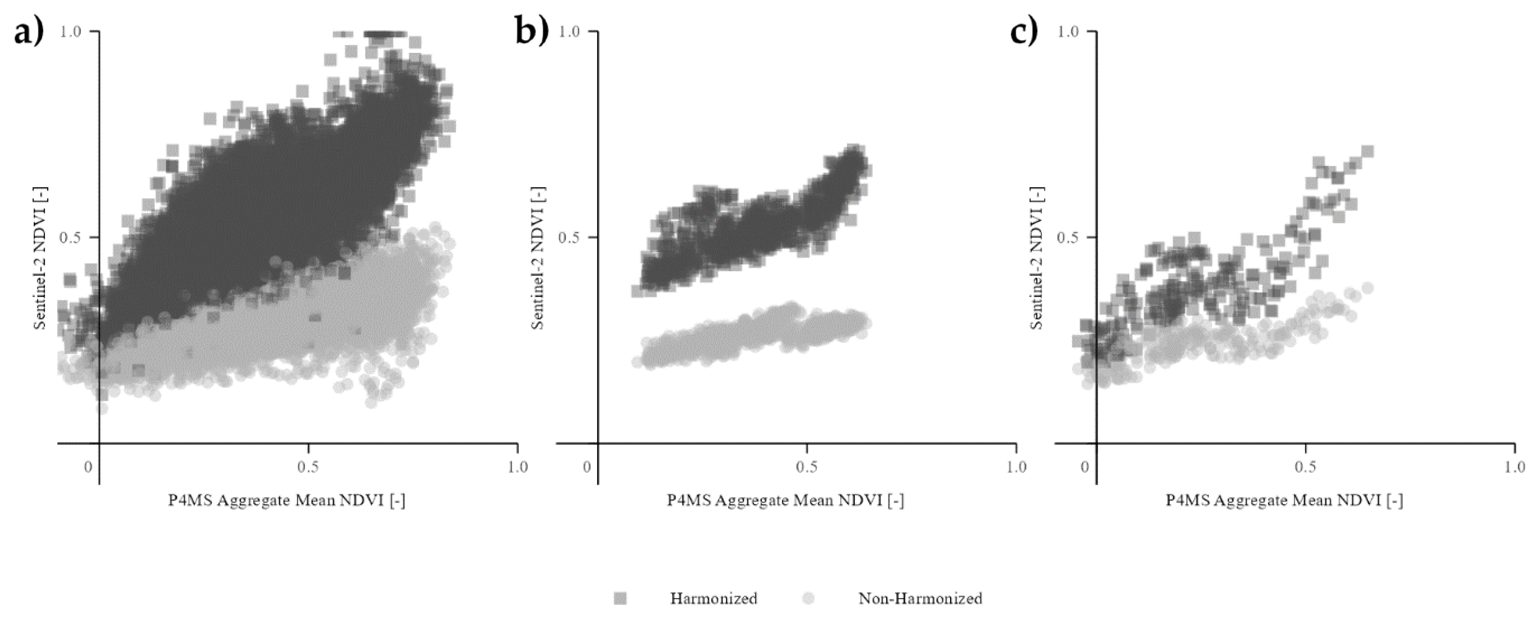
Analyzing the two sub-regions that can be clearly identified in the study area (Figure 2), the three scatterplots in Figure 11 reveal positive relationships between P4MS Aggregate Mean NDVI and S2 NDVI under both Harmonized and Non-Harmonized processing schemes. Across the entire study area (Figure 11a), P4MS values are, on average, 0.13 NDVI units lower than the Harmonized product and 0.13 units higher than the Non-Harmonized, producing two bands in the scatter where Harmonized points lie mostly above and Non-Harmonized mostly below the one-to-one line. The tighter clustering around the Harmonized line (SD ≈ 0.10) versus the broader spread with the Non-Harmonized (SD ≈ 0.13) underscores how harmonization reduces overall variability. In the shrubland sub-region (Figure 11b), where NDVI values are lower and vegetation is sparse, P4MS Aggregate Mean remains approximately 0.14 units below S2 Harmonized and 0.12 units above S2 Non-Harmonized. The scatter here is slightly more constrained for the Harmonized comparison (SD ≈ 0.09) than for the Non-Harmonized (SD ≈ 0.12). This alignment suggests that harmonization is particularly effective at capturing subtle greenness variations in low-cover environments, where uncorrected data would otherwise under-represent even modest changes in vegetation. Within the young eucalyptus sub-region (Figure 11c), P4MS NDVI underestimates Harmonized values by around 0.14 units (SD ≈ 0.11) but matches Non-Harmonized almost exactly on average (mean difference ≈ 0 units, SD ≈ 0.14). Here, the scatter reveals that S2 Harmonized NDVI is closer to a one-to-one agreement with P4MS, despite a slightly larger spread due to landscape heterogeneity (this area has patches of bare soil due to mobilization for the plantation). In contrast, the negligible mean offset with Non-Harmonized data masks the persistent structural bias in that product, which fails to capture the full greenness range of dense canopies.

4. Discussion

Understanding the complementary strengths of medium-resolution Sentinel-2 (S2) multispectral imagery (10 m) and high-resolution DJI Phantom 4 multispectral (P4MS) data (0.04 m) is important for scalable forest health monitoring. Results show strong seasonally coherent NDVI trajectories across platforms, but systematic offsets are likely tied to sensor design, atmospheric effects, and scale differences.
Although subtle, NDVI patterns reveal a consistent year-round upward trend, with both seasonal maximums (i.e., winter and spring) and seasonal minimums (i.e., summer and autumn) becoming higher in the second monitoring year than in the first. The growing mean NDVI values likely reflect an overall increase in the biomass density and greenness, which may result from vegetation recovery processes such as secondary regrowth and increased maturity, consistent with the expected characteristic phenology of post-fire Mediterranean landscapes: winter-spring green-up to peak greenness (December–June) driven by cool, moist conditions favoring shrub regrowth and herbaceous flush; and summer senescence (July–October) from water stress and dormancy [21,22].
The observed NDVI offsets between platforms must be contextualized against dominant variability sources like phenology and spatial resolution effects. Each S2 pixel (10 m resolution) aggregates signals from approximately 250 P4MS pixels (0.04 m resolution), inherently smoothing sub-pixel heterogeneity and compressing dynamic range (P4MS: ~0.4 amplitude; S2 Harm: ~0.3; S2 No-Harm: ~0.1; Figure 4). The subtle recovery trend superimposed on these seasonal cycles remains consistent across platforms despite offsets but is orders of magnitude smaller than phenological amplitudes. This confirms that inter-platform differences, while systematic, do not obscure recovery signals when platforms are applied independently for relative trend analysis.
P4MS captures greater trend magnitude and variability through fine-scale heterogeneity, though it remains sensitive to micro-shadowing and illumination geometry; consequently, S2’s provides smoother, spatially aggregated signals that are better suited for landscape-level monitoring. In longer-term studies, the effects of climatic conditions and, in particular, drought patterns on post-fire vegetation recovery can also be observed through NDVI changes [21,22]. The predominance of slow-growing species associated with natural post-fire succession (e.g., Cistus psilosepalus, Agrostis truncatula, and Cistus ladanifer) reflects the unique climatic and ecological conditions of this fire-affected landscape. The study area, representing a Mediterranean shrubland ecosystem five to seven years post-fire, demonstrates recovery patterns consistent with established trajectories for moderate to high fire severity areas [23,24].
The observed similarity in NDVI trends between UAS and satellite datasets aligns with findings from other authors, demonstrating that both satellite-derived and UAV-based multispectral imagery can detect similar large-scale patterns [3,25,26]. However, the UAS scenes reveal fine-scale heterogeneity, narrow disturbance features (e.g., tracks, planting rows), and small regeneration patches that are either spatially aliased or smoothed at 10 m in Sentinel-2 (Figure 6). These features are also evident as consistent spatial patterns in the NDVI difference maps across seasons (Figure 8 and Figure 9), confirming that satellite pixels aggregate UAS signals that vary systematically with phenology. This means that UAS data do not duplicate satellite information but rather resolve within-pixel variability that is critical for detecting localized degradation, early stress signals, and microsite recovery patterns, especially in semi-arid and fire-affected shrublands where regrowth is highly patchy [27,28,29].
The consistently higher NDVI amplitude of P4MS compared to the S2 data suggests an apparent higher signal-to-noise ratio (Figure 3), primarily reflecting dynamic range compression from spatial resolution differences and spectral bandwidth effects [30,31,32]. The sensors from the two considered platforms have differences in the spectral values, particularly in the near-infrared band (Figure 3). The narrower spectral bandwidth of the P4MS in relation to S2 leads to more precise spectral measurements and, potentially, to more accurate vegetation index calculations [33]. The atmospheric absorption affecting satellite imagery—which is negligible for UAS data—can introduce uncertainties [31]. The coarser resolution of S2 integrates diverse sub-pixel signals (similarly to P4MS aggregation), compressing dynamic range, which is further exacerbated by Non-Harmonized offset. Mindful bit-depth scaling and awareness of offset reversal effects are needed to avoid loss of true variability. UAS-based sensors are capable of capturing cleaner signals, especially in heterogeneous landscapes (as the sub-area analysis suggests, Figure 11), due to their finer resolution [30,32].
The higher P4MS NDVI variability reflects the ability to resolve individual plants or bare soil patches as individual pixels. In contrast, S2’s coarser resolution integrates signals from multiple surface types, reducing variability. Aggregated 10 m P4MS maps retained key NDVI gradients observed in the 0.04 m resolution (Figure 6), confirming that rescaling can conserve first-order spatial signals when patch sizes exceed ¼ of the aggregation kernel. However, fine-scale variability—such as seedling clusters in the eucalyptus sub-area—was lost after aggregation, supporting that S2 can obscure vital regeneration hotspots in early post-fire years [34]. The larger scatter and offset in shrubland pixels than in planted eucalyptus rows (as seen in the scatterplots in Figure 11) is consistent with mixed-pixel dilution documented in other studies [35]. Sub-area analysis reveals cover-type influences on platform coherence (Figure 11). Shrubland exhibits greater inter-platform NDVI difference scatter than uniform eucalyptus plantation, likely due to mixing diverse finer-scale vegetation patches with bare soil. In contrast, eucalyptus maintains homogeneous tree cover along structured rows despite comparable soil exposure. Uniform eucalyptus rows produce less sub-pixel variability, creating a narrower true NDVI range that aligns better with Non-Harmonized S2’s radiometric compression, indicating vegetation patterning modulates scale effects.
As verified in the example shown in Figure 10, the lower sun elevation angles during winter may significantly affect the quality and interpretability of remote sensing imagery. As the sun angle decreases, longer shadows cast by terrain and vegetation can obscure surface features and distort spectral signatures. Additionally, reduced incident radiation at lower sun angles diminishes the signal-to-noise ratio, weakening the overall data quality and amplifying noise effects. These challenges are further compounded by radiometric offsets in some datasets, which can introduce artifacts such as clipping in shadowed areas [35]. Such artifacts obscure subtle spectral variations and may compromise the accuracy of vegetation indices or land cover classifications [36]. Moreover, the seasonal variation in shadowing and processing artifacts complicates time-series analyses, introducing inconsistencies in the study of vegetation dynamics or land cover changes [37]. Careful consideration of these effects is essential for accurate interpretation of datasets, particularly when analyzing seasonal or multi-temporal changes.
Harmonized S2 is generally preferable for post-fire shrubland monitoring spanning processing baseline changes (pre-/post-04.00), ensuring temporal consistency critical for long-term recovery trends. However, in complex terrain like our study site—with winter acquisitions under low illumination angles—the Harmonized series produces RED = 0 clipping, resulting in NDVI = 1 artifacts in shadowed pixels (Figure 10; absent in Non-Harmonized, Figure A2). This apparently stronger Harmonized signal reflects a rescaled dynamic range from offset reversal. Non-Harmonized avoids these artifacts without dedicated masking. For our site, Non-Harmonized proved more reliable overall.
Satellite and UAS imagery each offer distinct advantages and limitations for vegetation monitoring. Satellite systems like S2 provide consistent, regular data acquisition, making them ideal for long-term, spatially aggregated vegetation dynamics. However, their relatively lower spatial resolution can limit the detection of fine-scale vegetation features, and the data is highly susceptible to atmospheric conditions, requiring complex corrections to ensure accuracy. Pixel-level cloud masks (S2 SCL) could provide superior scene selection compared to the 15% scene cloud cover threshold adopted in this study. However, SCL cloud shadows and cloud edges remain classification challenges that may compromise SLC classification accuracy [20,38]. and particular care should be taken when dealing with heavily cloud-covered scenes. In contrast, UAS operate at much lower altitudes, achieving significantly higher spatial resolutions that allow for detailed detection of vegetation characteristics. Since they are largely unaffected by atmospheric interference, UAS data do not require atmospheric corrections, adding to their application for localized studies.

5. Conclusions

This study demonstrates that both satellite-based (Sentinel-2) and UAS-derived (P4MS) high-resolution multispectral imagery capture broadly consistent seasonal patterns and vegetation dynamics in Mediterranean shrubland ecosystems, though differences emerge depending on spatial scale and vegetation structure.
The results show that while coarser satellite data effectively tracks broad temporal trends and landscape-level changes, with better cross-platform coherence in uniform canopies than heterogeneous shrublands, UAS systems offer detailed insight into fine-scale spatial heterogeneity, regeneration patches, and local disturbance responses that may be missed or diluted at the satellite scale—especially in areas with sparse or heterogeneous cover. Rigorous processing workflows are necessary to minimize bias when comparing indices like NDVI across platforms. Radiometric offset differences spanning from processing baseline changes, such as those demonstrated to affect Sentinel-2, require mindful bit-depth scaling to preserve variability. Resampling methods bridge resolution gaps.
Given the overall coherence between satellite and UAS observations, the choice of platform can be tailored to specific management or research needs. For long-term monitoring of vegetation dynamics, Sentinel-2 provides consistent trajectories and spatial patterns at the landscape scale, particularly in contexts where continuous UAS acquisition is not feasible. Sentinel-2 NDVI can also serve as an accessible, spatially continuous input variable for regional ecosystem modelling applications. Conversely, for site-specific management, such as restoration planning, early stress detection, or prioritizing interventions, UAS imagery adds critical value by revealing sub-decametric patterns and microhabitat variability. The findings of this study support the strategic selection of remote sensing approaches based on monitoring objectives, ecosystem characteristics, and resource constraints, and highlight the utility of both platforms for robust environmental modelling and effective management of Mediterranean ecosystems recovering from disturbance.

Author Contributions

E.R.O.: Data curation; Formal analysis; Investigation; Methodology; Validation; Visualization; Writing—original draft; Writing—review and editing. T.v.d.W.d.S.: Data curation, Formal analysis; Investigation; Writing—review and editing. L.M.G.P.: Conceptualization; Data curation; Formal analysis; Methodology; Software; Supervision; Validation; Writing—review and editing. N.V.: Conceptualization; Formal analysis; Methodology; Writing—review and editing. J.J.K.: Conceptualization; Funding Acquisition; Software; Writing—review and editing. B.R.F.O.: Conceptualization; Data curation; Funding acquisition; Investigation; Methodology; Project administration; Resources; Supervision; Validation; Visualization; Writing—review and editing. All authors have read and agreed to the published version of the manuscript.

Funding

This research was funded by ModelEco (PTDC/ASP-SIL/3504/2020) http://doi.org/10.54499/PTDC/ASP-SIL/3504/2020, funded by national funds (OE) through FCT/MCTES. Tiago van der Worp Silva was funded by national funds through FCT—Fundação para a Ciência e Tecnologia, I.P. in the form of a Ph.D. Grant [2023.01767.BDANA]. Bruna R. F. Oliveira was funded by national funds through the Portuguese Foundation for Science and Technology, I.P., and by FEDER COMPETE 2020 funds, in the scope of the Stimulus for Scientific Employment—Individual Call [2021. 00785.CEECIND], (doi.org/10.54499/2021.00785.CEECIND/CP1659/CT0028).

Data Availability Statement

Data can be made available upon request by email to the corresponding author.

Acknowledgments

The authors acknowledge financial support to CESAM by national funds through FCT—Fundação para a Ciência e a Tecnologia I.P., under the project/grant UID/50006 + LA/P/0094/2020.

Conflicts of Interest

The authors declare no conflicts of interest.

Appendix A

Figure A1. NDVI difference boxplots, calculated as P4MS Aggregate Mean minus coeval Sentinel-2 Non-Harmonized observations, according to four seasonal examples.
Land 15 00306 g0a1
Figure A2. Scenes from 20-Dec-2023, including: (a) surface reflectance values of Band 4 from S2 Non-Harmonized (with reflectance = 0 in purple); (b) NDVI values from S2 Non-Harmonized (with NDVI = 1 in green-ish-cyan); and (c) NDVI difference values between P4MS Aggregate Mean and S2 Non-Harmonized.
Land 15 00306 g0a2

References

  1. Wang, R.; Sun, Y.; Zong, J.; Wang, Y.; Cao, X.; Wang, Y.; Cheng, X.; Zhang, W. Remote Sensing Application in Ecological Restoration Monitoring: A Systematic Review. Remote Sens. 2024, 16, 2204. [Google Scholar] [CrossRef]
  2. Sun, Z.; Wang, X.; Wang, Z.; Yang, L.; Xie, Y.; Huang, Y. UAVs as Remote Sensing Platforms in Plant Ecology: Review of Applications and Challenges. J. Plant Ecol. 2021, 14, 1003–1023. [Google Scholar] [CrossRef]
  3. Li, M.; Shamshiri, R.R.; Weltzien, C.; Schirrmann, M. Crop Monitoring Using Sentinel-2 and UAV Multispectral Imagery: A Comparison Case Study in Northeastern Germany. Remote Sens. 2022, 14, 4426. [Google Scholar] [CrossRef]
  4. Senf, C. Seeing the System from Above: The Use and Potential of Remote Sensing for Studying Ecosystem Dynamics. Ecosystems 2022, 25, 1719–1737. [Google Scholar] [CrossRef]
  5. Ryu, J.H.; Moon, H.D.; Do Lee, K.; Cho, J.; Ahn, H.Y. Evaluation of Surface Reflectance and Vegetation Indices Measured by Sentinel-2 Satellite Using Drone Considering Crop Type and Surface Heterogeneity. Korean J. Remote Sens. 2024, 40, 657–673. [Google Scholar] [CrossRef]
  6. Isaev, E.; Kulikov, M.; Shibkov, E.; Sidle, R.C. Bias Correction of Sentinel-2 with Unmanned Aerial Vehicle Multispectral Data for Use in Monitoring Walnut Fruit Forest in Western Tien Shan, Kyrgyzstan. J. Appl. Remote Sens. 2022, 17, 22204. [Google Scholar] [CrossRef]
  7. del Río-Mena, T.; Willemen, L.; Vrieling, A.; Nelson, A. How Remote Sensing Choices Influence Ecosystem Services Monitoring and Evaluation Results of Ecological Restoration Interventions. Ecosyst. Serv. 2023, 64, 101565. [Google Scholar] [CrossRef]
  8. Mehmood, K.; Anees, S.A.; Muhammad, S.; Hussain, K.; Shahzad, F.; Liu, Q.; Ansari, M.J.; Alharbi, S.A.; Khan, W.R. Analyzing Vegetation Health Dynamics across Seasons and Regions through NDVI and Climatic Variables. Sci. Rep. 2024, 14, 11775. [Google Scholar] [CrossRef]
  9. Gutman, G.; Skakun, S.; Gitelson, A. Revisiting the Use of Red and Near-Infrared Reflectances in Vegetation Studies and Numerical Climate Models. Sci. Remote Sens. 2021, 4, 100025. [Google Scholar] [CrossRef]
  10. Pastonchi, L.; Di Gennaro, S.F.; Toscano, P.; Matese, A. Comparison between Satellite and Ground Data with UAV-Based Information to Analyse Vineyard Spatio-Temporal Variability. Oeno One 2020, 54, 919–934. [Google Scholar] [CrossRef]
  11. Alvarez-Vanhard, E.; Corpetti, T.; Houet, T. UAV & Satellite Synergies for Optical Remote Sensing Applications: A Literature Review. Sci. Remote Sens. 2021, 3, 100019. [Google Scholar]
  12. Kottek, M.; Grieser, J.; Beck, C.; Rudolf, B.; Rubel, F. World Map of the Köppen-Geiger Climate Classification Updated. Meteorol. Z. 2006, 15, 259–263. [Google Scholar] [CrossRef]
  13. ICNF. 10.o Relatório Provisório de Incêndios Florestais—2017; ICNF: Alpharetta, GA, USA, 2017. [Google Scholar]
  14. EFFIS. Copernicus—Emergency Management Service. European Forest Fire Information System. Available online: https://effis.jrc.ec.europa.eu/ (accessed on 19 September 2017).
  15. da Silva, T.v.d.W.; Gomes Pereira, L.; Oliveira, B.R.F. Assessing Geometric and Radiometric Accuracy of DJI P4 MS Imagery Processed with Agisoft Metashape for Shrubland Mapping. Remote Sens. 2024, 16, 4633. [Google Scholar] [CrossRef]
  16. ESA. Sentinel-2 User Handbook; ESA: Paris, France, 2015; Volume Rev2. [Google Scholar]
  17. Amani, M.; Ghorbanian, A.; Ahmadi, S.A.; Kakooei, M.; Moghimi, A.; Mirmazloumi, S.M.; Moghaddam, S.H.A.; Mahdavi, S.; Ghahremanloo, M.; Parsian, S.; et al. Google Earth Engine Cloud Computing Platform for Remote Sensing Big Data Applications: A Comprehensive Review. IEEE J. Sel. Top. Appl. Earth Obs. Remote Sens. 2020, 13, 5326–5350. [Google Scholar] [CrossRef]
  18. ESA. S2 Processing. Available online: https://sentiwiki.copernicus.eu/web/s2-processing (accessed on 10 January 2026).
  19. ESRI. ArcGIS Pro Geoprocessing Tool Reference. Available online: https://pro.arcgis.com/en/pro-app/latest/tool-reference/main/arcgis-pro-tool-reference.htm (accessed on 10 January 2026).
  20. Louis, J.; Pflug, B.; Debaecker, V.; Mueller-Wilm, U.; Iannone, R.Q.; Boccia, V.; Gascon, F. Evolutions of Sentinel-2 Level-2a Cloud Masking Algorithm Sen2Cor Prototype First Results. In 2021 International Geoscience and Remote Sensing Symposium (IGARSS); IEEE: New York, NY, USA, 2021; pp. 3041–3044. [Google Scholar] [CrossRef]
  21. Blanco-Rodríguez, M.Á.; Ameztegui, A.; Gelabert, P.; Rodrigues, M.; Coll, L. Short-Term Recovery of Post-Fire Vegetation Is Primarily Limited by Drought in Mediterranean Forest Ecosystems. Fire Ecol. 2023, 19, 68. [Google Scholar] [CrossRef]
  22. Viana-Soto, A.; Aguado, I.; Salas, J.; García, M. Identifying Post-Fire Recovery Trajectories and Driving Factors Using Landsat Time Series in Fire-Prone Mediterranean Pine Forests. Remote Sens. 2020, 12, 1499. [Google Scholar] [CrossRef]
  23. Ortega, M.; Lora, Á.; Yocom, L.; Zumaquero, R.; Molina, J.R. Effects of Fire Recurrence and Severity on Mediterranean Vegetation Dynamics: Implications for Structure and Composition in Southern Spain. Sci. Total Environ. 2025, 961, 178392. [Google Scholar] [CrossRef] [PubMed]
  24. Peris-Llopis, M.; Vastaranta, M.; Saarinen, N.; González-Olabarria, J.R.; García-Gonzalo, J.; Mola-Yudego, B. Post-Fire Vegetation Dynamics and Location as Main Drivers of Fire Recurrence in Mediterranean Forests. For. Ecol. Manag. 2024, 568, 122126. [Google Scholar] [CrossRef]
  25. Thapa, S.; Garcia Millan, V.E.; Eklundh, L. Assessing Forest Phenology: A Multi-Scale Comparison of near-Surface (UAV, Spectral Reflectance Sensor, Phenocam) and Satellite (MODIS, Sentinel-2) Remote Sensing. Remote Sens. 2021, 13, 1597. [Google Scholar] [CrossRef]
  26. Bollas, N.; Kokinou, E.; Polychronos, V. Comparison of Sentinel-2 and Uav Multispectral Data for Use in Precision Agriculture: An Application from Northern Greece. Drones 2021, 5, 35. [Google Scholar] [CrossRef]
  27. Abdullah, M.M.; Al-Ali, Z.M.; Blanton, A.; Charabi, Y.; Abulibdeh, A.; Al-Awadhi, T.; Srinivasan, S.; Fadda, E.; Mohan, M. UAVs for Improving Seasonal Vegetation Assessment in Arid Environments. Front. Environ. Sci. 2024, 12, 1366712. [Google Scholar] [CrossRef]
  28. Bousquet, E.; Mialon, A.; Rodriguez-Fernandez, N.; Mermoz, S.; Kerr, Y. Monitoring Post-Fire Recovery of Various Vegetation Biomes Using Multi-Wavelength Satellite Remote Sensing. Biogeosciences 2022, 19, 3317–3336. [Google Scholar] [CrossRef]
  29. Ogungbuyi, M.G.; Mohammed, C.; Fischer, A.M.; Turner, D.; Whitehead, J.; Harrison, M.T. Integration of Drone and Satellite Imagery Improves Agricultural Management Agility. Remote Sens. 2024, 16, 4688. [Google Scholar] [CrossRef]
  30. Sozzi, M.; Kayad, A.; Gobbo, S.; Cogato, A.; Sartori, L.; Marinello, F.; Singh, V.; Huang, Y. Economic Comparison of Satellite, Plane and UAV-Acquired NDVI Images for Site-Specific Nitrogen Application: Observations from Italy. Agronomy 2021, 11, 2098. [Google Scholar] [CrossRef]
  31. Moravec, D.; Komárek, J.; Medina, S.L.C.; Molina, I. Effect of Atmospheric Corrections on NDVI: Intercomparability of Landsat 8, Sentinel-2, and UAV Sensors. Remote Sens. 2021, 13, 3550. [Google Scholar] [CrossRef]
  32. Gati, B. Comparison of Vegetation Indices Obtained by Drone and Satellite. In E3S Web of Conferences; EDP Sciences: London, UK, 2024; Volume 590, p. 01008. [Google Scholar] [CrossRef]
  33. Martinez, J.L.; Lucas-borja, M.E.; Plaza-alvarez, P.A.; Denisi, P.; Moreno, M.A.; Hernández, D.; González-romero, J.; Zema, D.A. Comparison of Satellite and Drone-based Images at Two Spatial Scales to Evaluate Vegetation Regeneration after Post-fire Treatments in a Mediterranean Forest. Appl. Sci. 2021, 11, 5423. [Google Scholar] [CrossRef]
  34. Wang, H.; Muller, J.D.; Tatarinov, F.; Yakir, D.; Rotenberg, E. Disentangling Soil, Shade, and Tree Canopy Contributions to Mixed Satellite Vegetation Indices in a Sparse Dry Forest. Remote Sens. 2022, 14, 3681. [Google Scholar] [CrossRef]
  35. Galvao, L.S.; Ponzoni, F.J.; Epiphanio, J.C.N.; Rudorff, B.F.T.; Formaggio, A.R. Sun and View Angle Effects on NDVI Determination of Land Cover Types in the Brazilian Amazon Region with Hyperspectral Data. Int. J. Remote Sens. 2004, 25, 1861–1879. [Google Scholar] [CrossRef]
  36. Oliveira, E.R.; Disperati, L.; Cenci, L.; Pereira, L.G.; Alves, F.L. Multi-Index Image Differencing Method (MINDED) for Flood Extent Estimations. Remote Sens. 2019, 11, 1305. [Google Scholar] [CrossRef]
  37. Alavipanah, S.K.; Karimi Firozjaei, M.; Sedighi, A.; Fathololoumi, S.; Zare Naghadehi, S.; Saleh, S.; Naghdizadegan, M.; Gomeh, Z.; Arsanjani, J.J.; Makki, M.; et al. The Shadow Effect on Surface Biophysical Variables Derived from Remote Sensing: A Review. Land 2022, 11, 2025. [Google Scholar] [CrossRef]
  38. Zekoll, V.; Main-Knorn, M.; Alonso, K.; Louis, J.; Frantz, D.; Richter, R.; Pflug, B. Comparison of Masking Algorithms for Sentinel-2 Imagery. Remote Sens. 2021, 13, 137. [Google Scholar] [CrossRef]
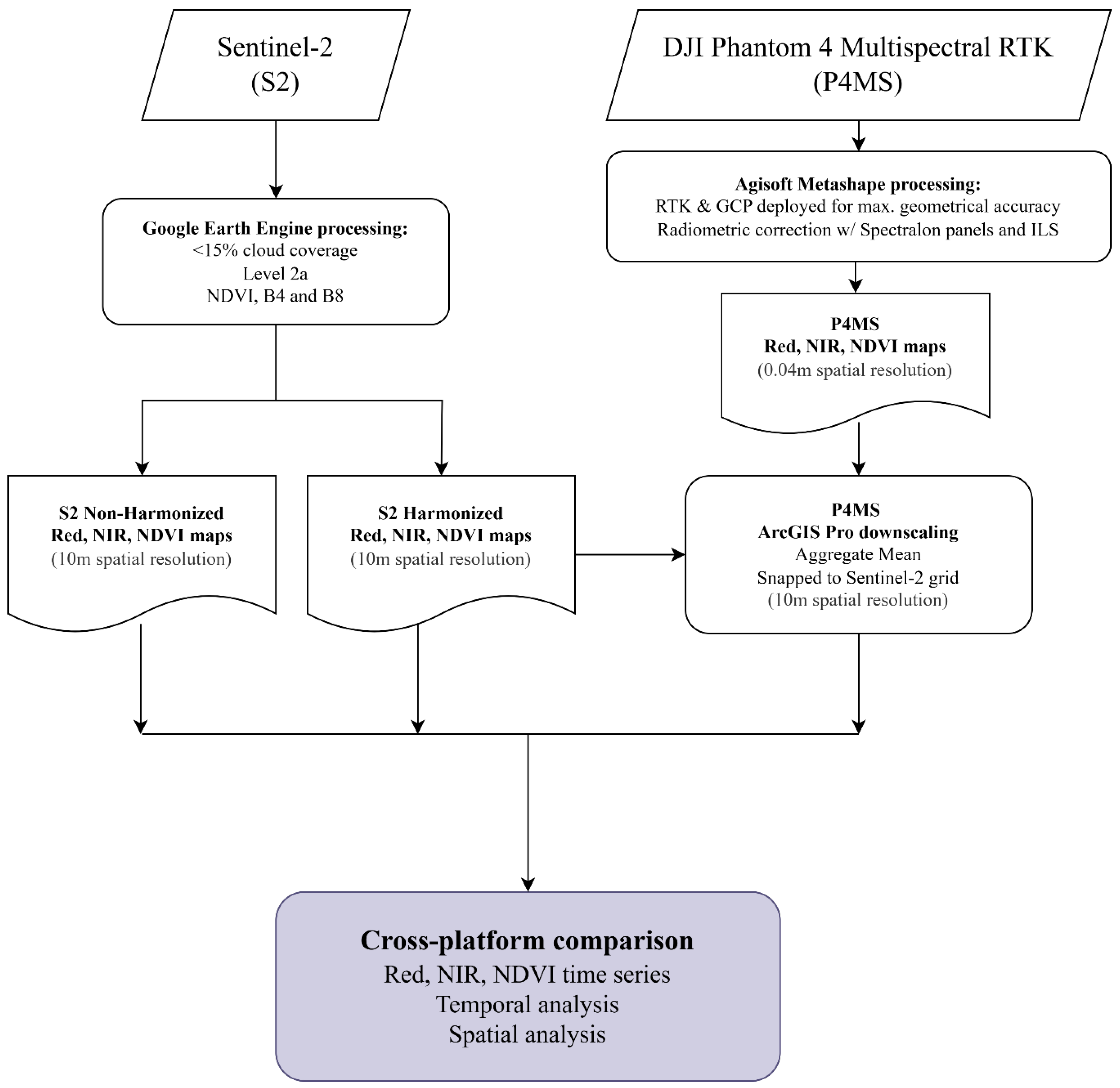
Figure 1. Flow Diagram of the Methodology for Cross-Platform Comparison of NDVI-Based Vegetation Monitoring.
Land 15 00306 g001
Figure 2. Location of the study area and corresponding sub-areas. (Background composition: Phantom 4 Multispectral RTK true color RGB—20 December 2023; Reference Coordinate System: WGS84).
Land 15 00306 g002
Figure 3. Multispectral band setup of P4MS and S2 (with 10 m spatial resolution) sensors within the visible and NIR range.
Land 15 00306 g003
Figure 4. Mean values of NDVI timeseries, obtained for the whole study area), according to different datasets: S2 Harmonized, S2 Non-Harmonized, and P4MS (with “×” highlighting two outlier points for each S2 dataset).
Land 15 00306 g004
Figure 5. Scenes associated with clouds/cloud shadows (from 19-Apr-2022 and 3-Jun-2023), represented as (a) S2 Harmonized NDVI and (b) S2 Scene Classification Layer (SCL).
Land 15 00306 g005
Figure 6. Consecutive seasonal coeval NDVI maps from Oct-2022, Feb-2023, Apr-2023, and July-2023 (Autumn to Summer), acquired by Sentinel-2 Harmonized, S2 Non-Harmonized, P4MS, and P4MS Aggregate Mean. The two insets (on the left) include a pathway intersection and young eucalyptus plantation location, highlighting the differences of spatial resolution between satellite (Sentinel-2 Harmonized) and UAV (P4MS) platforms.
Land 15 00306 g006
Figure 7. Boxplots of reflectance differences between rescaled P4MS and S2 MSI sensors across equivalent Red and NIR bands for four seasonal scenes (from October 2022 to July 2023), relative to (a) Harmonized and (b) the Non-Harmonized series.
Land 15 00306 g007
Figure 8. NDVI difference maps calculated as P4MS Aggregate Mean minus coeval Sentinel-2 Harmonized observations. Panels show seasonal examples: (a) Autumn, (b) Winter, (c) Spring, and (d) Summer. Panels (e,f) present the mean and standard deviation of NDVI differences across the entire time series, respectively.
Land 15 00306 g008
Figure 9. NDVI difference maps calculated as P4MS Aggregate Mean minus coeval Sentinel-2 Non-Harmonized observations. Panels show seasonal examples: (a) Autumn, (b) Winter, (c) Spring, and (d) Summer. Panels (e,f) present the mean and standard deviation of NDVI differences across the entire time series, respectively.
Land 15 00306 g009
Figure 10. Scenes from 20-Dec-2023, including: (a) surface reflectance values of Band 4 (Red) from S2 Harmonized (with reflectance = 0 in purple); and (b) NDVI values from S2 Non-Harmonized (with NDVI = 1 in greenish-cyan).
Land 15 00306 g010
Figure 11. Scatterplots of coeval Normalized Difference Vegetation Index (NDVI) values comparing P4MS Aggregate Mean NDVI with Sentinel-2 Harmonized and Sentinel-2 Non-Harmonized for (a) the entire study area (n = 16,614), (b) the shrubland sub-region (n = 858), and (c) the eucalyptus sub-region (n = 234).
Land 15 00306 g011
Table 1. Summary of the processed P4MS scenes, alongside the closest available coeval Sentinel-2 (S2) scenes. In bold—most coeval pairs; (*) scenes affected by clouds.
P4MSS2∆t [Days]P4MSS2∆t [Days]P4MSS2∆t [Days]
-19-Apr-2022 (*)--5-Nov-2022-20-Jul-202318-Jul-2023−2
21-Apr-202229-Apr-20228-10-Nov-2022--23-Jul-2023-
-4-May-2022--25-Nov-2022--28-Jul-2023-
-14-May-2022-11-Jan-20234-Jan-2023−7-7-Aug-2023-
-13-Jun-2022--24-Jan-2023--12-Aug-2023-
-28-Jun-2022--29-Jan-2023--17-Aug-2023-
-3-Jul-2022--3-Feb-2023--22-Aug-2023-
7-Jul-20228-Jul-2022116-Feb-202323-Feb-202377-Sep-20231-Sep-2023−6
-18-Jul-2022--28-Feb-2023--26-Sep-2023-
-23-Jul-2022--15-Mar-2023--1-Oct-2023-
29-Jul-202228-Jul-2022−130-Mar-202325-Mar-2023−5-25-Nov-2023-
-2-Aug-2022--4-Apr-2023-20-Dec-202320-Dec-20230
-7-Aug-2022--9-Apr-2023--24-Jan-2024-
-12-Aug-2022-20-Apr-202319-Apr-2023−1-3-Feb-2024-
-17-Aug-2022--24-Apr-2023-19-Mar-202419-Mar-20240
-22-Aug-2022--14-May-2023--23-Apr-2024-
-27-Aug-2022--19-May-2023--8-May-2024-
-1-Sep-2022--3-Jun-2023 (*)--23-May-2024-
-11-Sep-2022-22-Jun-202323-Jun-20231-28-May-2024-
-26-Sep-2022--28-Jun-2023--2-Jun-2024-
-1-Oct-2022--3-Jul-2023--12-Jun-2024-
6-Oct-202211-Oct-20225-13-Jul-2023-20-Jun-202422-Jun-20242
Table 2. Summary statistics of the NDVI difference maps between P4MS Aggregate Mean and the coeval Sentinel 2 Harmonized and Non-Harmonized maps. n = 1278 10-m pixels.
(P4MS AgMean)—(S2 Harmonized)(P4MS AgMean)—(S2 Non-Harmonized)
Oct-2022Feb-2023Apr-2023Jul-2023Oct-2022Feb-2023Apr-2023Jul-2023
Mean−0.297−0.043−0.154−0.0820.0020.2810.1050.144
Median−0.304−0.047−0.160−0.0840.0060.2850.1090.144
Std. Dev.0.0730.0580.0600.0720.0810.0620.0700.089
Min−0.536−0.261−0.340−0.325−0.301−0.014−0.236−0.235
Max0.0580.2580.1300.1720.2800.4520.3390.382
Sum−380.198−55.403−196.406−104.2551.957359.576133.930184.138
Skewness0.7901.0160.8300.187−0.172−0.609−0.401−0.179
Kurtosis5.1987.5035.2892.9053.1894.4683.9463.232
Disclaimer/Publisher’s Note: The statements, opinions and data contained in all publications are solely those of the individual author(s) and contributor(s) and not of MDPI and/or the editor(s). MDPI and/or the editor(s) disclaim responsibility for any injury to people or property resulting from any ideas, methods, instructions or products referred to in the content.