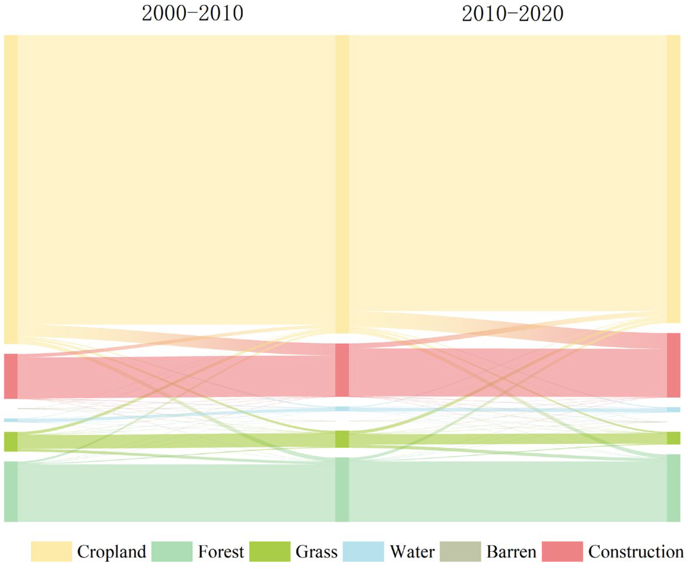
2.3.1. Land Use and Land Cover Change
Within a specific time interval, the land use dynamic degree model quantifies the rate at which land use quantities change in a study area. The single land use dynamic degree specifically measures the areal change rate of individual land use types within a region during the same period.
reflects the dynamic degree of a specific land use type over the study period. and represent the area at the beginning and end of this period, respectively, and indicates its duration. A positive K value (K > 0) indicates an increase in the area of the land use type over time.
The land use transition matrix is a two-dimensional matrix derived from the changing relationships of land-cover conditions at different times within the same area, reflecting the conversion between different land use types [
38]. Numerous scholars have utilized this model to analyze land use changes, where
represents the area of land use type
i that transitions to land use type
j, and
n denotes the number of land use types.
2.3.2. Multi-Scenario Simulation of Urban Expansion
Traditional cellular automata (CA) models often struggle to simulate the synchronous evolution of land use patches and fail to capture complex land conversion rules. To address these limitations, the PLUS model integrates CA with a random forest algorithm and an adaptive inertia competition mechanism. This integration improves the model’s ability to identify land use drivers and enhances patch-scale simulation accuracy. The PLUS model first extracts the expanded land parcels between the two periods. Subsequently, development probabilities for each land category are estimated using a random forest method, after which a CA module with varied random patch seeds is used to simulate future landscape evolution.
First, based on the relevant existing studies [
39,
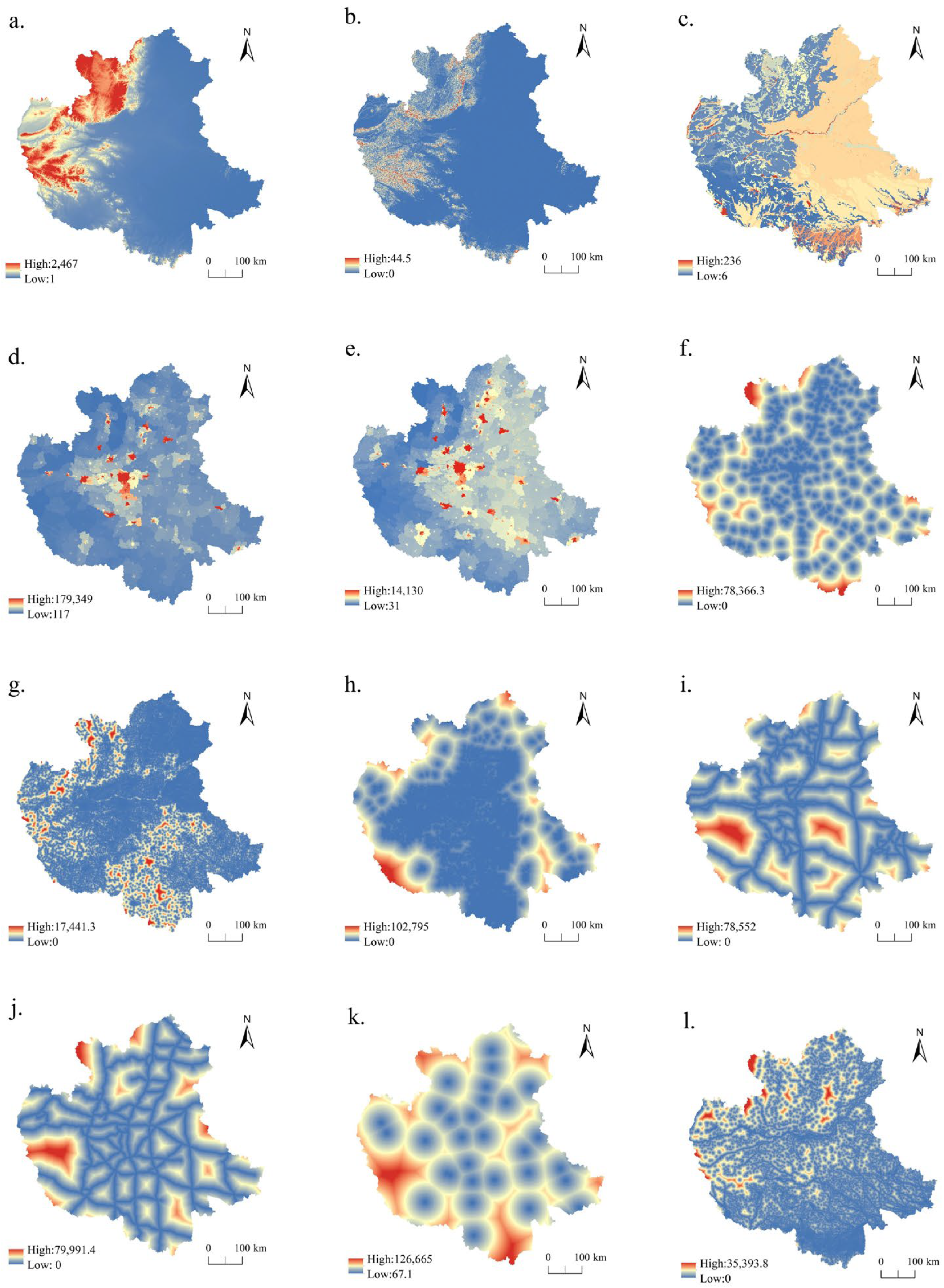
40], the practical conditions of the CPUA, and the availability of data, 12 driving factors were selected from three aspects: basic geographic information, socioeconomic elements, and transportation accessibility. These include elevation, slope, soil type, GDP, population, distance to primary roads, distance to secondary roads, distance to tertiary roads, distance to railways, distance to highways, distance to city center, and distance to water bodies. All the datasets were converted to raster format and unified to match the projection coordinate system and spatial resolution of the land cover data. Second, the Land Expansion Analysis Strategy (LEAS) module of the PLUS model was used to calculate the development probabilities of different land use types in the study area. Finally, by integrating the target cell counts for each land type, the transition cost matrix, and the probabilities for generating patch seeds, and neighborhood factors, a land use change simulation was conducted using the multi-type random patch seed-based CA model embedded in the PLUS framework.
- (1)
Neighborhood Factor Weights: The neighborhood factor describes the interactions among different land use types and land units within a defined neighborhood. Their weights range from zero to one. A higher weight indicates that the land use type is more resistant to transformation and possesses a stronger capacity for expansion. In contrast, a lower weight suggests that the land use type is more likely to be converted or replaced by other land use categories.
where
is the expansion area change of land use type
i, and
and
represent the minimum and maximum expansion area changes among all land use types, respectively [
41].
This study utilized land use data from 2010 and 2020 and obtained the neighborhood factor weights as shown in
Table 2 based on the results of the Markov chain analysis. In the weight calculation, setting the weight of cropland to 0 was deemed inconsistent with practical conditions; therefore, the weight for cropland was adjusted to 0.1.
- (2)
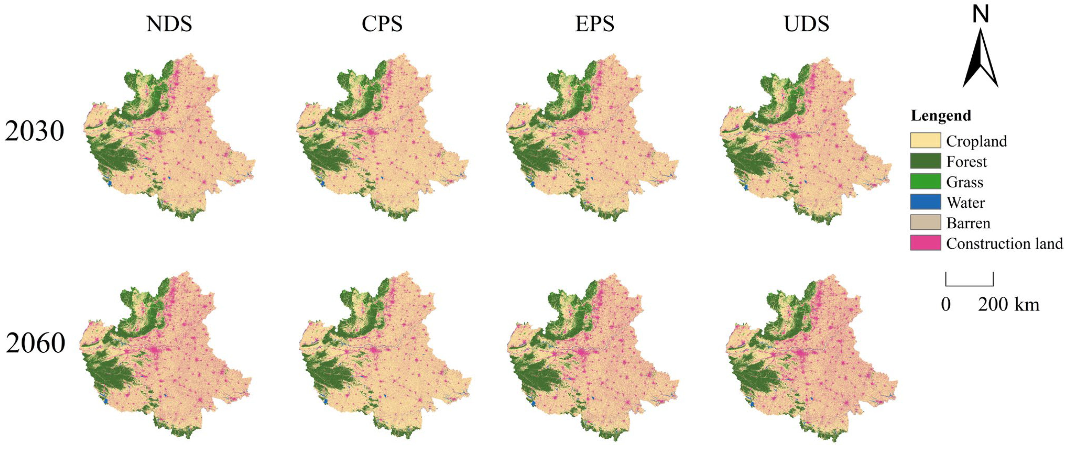
Scenario Setting: Using land use data from 2000, 2010, and 2020 for the CPUA, land use in 2030 and 2060 was simulated under multiple scenarios, including natural development, ecological protection, cropland protection, and urban development. The Markov chain model was applied to constrain land use quantities by controlling the transition probabilities between categories, enabling the projection of land use distributions under different scenarios [
42].
Natural development scenario: The NDs assume that the urban agglomeration maintains the land use change dynamics identified during 2000–2020, reflecting current urbanization trends. This scenario does not impose any restrictions on land use transitions or consider government or market interventions, serving as the baseline for simulating land use changes without additional constraints.
Ecological protection scenario: EPs aim to maximize the ecological benefits provided by various land use types. High population density and economic activities in the CPUA have already caused significant existing and potential ecological damage. This scenario emphasizes ecological protection as a priority for further optimizing the development of the region. Based on previous studies and actual conditions [
43], this scenario reduces the transition probability from forestland and grassland to construction land by 50% and from cropland to construction land by 30%, and increases cropland-to-forest/grassland probability by 30%. Additionally, it treats regional water bodies as a constraint and prohibits any land use change.
Cropland protection scenario: The quantity and quality of prime cropland are crucial for national food security, and the CPUA is an important grain-producing region in China. Therefore, land use change simulations must incorporate cropland protection into the baseline scenario. Protecting croplands in urban agglomerations requires strict control of the conversion of prime cropland to other land use types to prevent its loss during urbanization, thereby maintaining the total area of prime cropland. In the scenario setting, the probability of transitioning from cropland to construction land was reduced by 60%, thereby ensuring strict cropland protection.
Urban development scenario: Rapid economic growth drives continuous urbanization. In the UD scenario, the transition probabilities from cropland, forest land, and grassland to construction land were reduced by 20%, whereas the transition probabilities from construction land to other land types, excluding cropland, were reduced by 30%.
For each development scenario, a cost matrix was established to represent the transitions between different land use types, where 1 indicates allowed conversion and 0 indicates prohibited conversion. In
Table 3, A, B, C, D, E, and F represent the cropland, forest, grass, water, barren land, and construction land, respectively.
- (3)
Driving factor settings: For future simulations, this study employed the LEAS and multi-type random patch seed (CARS) method, driven by a CA-Markov model, to generate the probability matrix of future land use demand. The LEAS analyzes historical land expansion trends and transforms them into predictive demands under different future scenarios. The CARS method simulates spatial patterns among different land use types by randomly generating seed patches.
The key driving factors incorporated into the model included the digital elevation model (DEM), slope, soil type, population, GDP, distance to expressways, distance to city centers, and distance to major roads (including primary, secondary, and tertiary roads).
Figure 2 illustrates that all the raster datasets were standardized to a consistent spatial resolution and coordinate system.
2.3.3. Carbon Storage Calculation
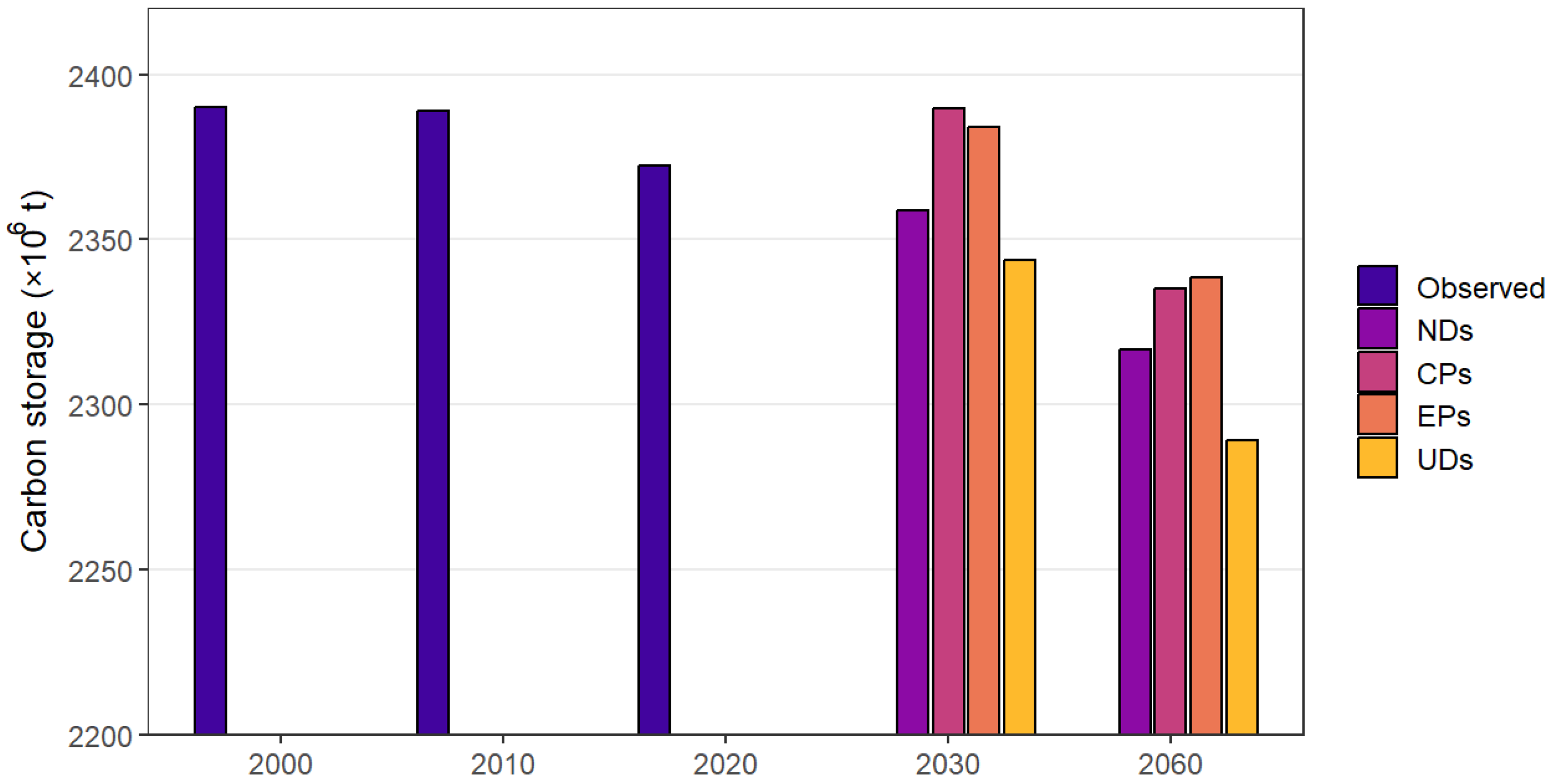
InVEST, developed by Stanford University, the World Wildlife Fund, and other organizations, is an open-source modeling tool designed to quantify the value of natural capital and ecosystem services. This study utilized the carbon storage module of the InVEST model to estimate carbon storage in the CPUA across different time periods. The carbon storage was calculated using the following formula:
where
represents the total carbon storage, and
,
,
, and
denote the carbon storage in the aboveground biomass, belowground biomass, soil, and dead organic matter, respectively.
Direct field measurements of carbon density in the CPUA are challenging and difficult to carry out. Therefore, the existing carbon density data were used for estimation and subsequently adjusted based on the specific climate conditions, soil properties, and land use types within the study area. Previous studies, both domestic and international, have demonstrated that aboveground and belowground biomass carbon densities are positively correlated with annual precipitation and mean annual temperature. Soil organic carbon has also been shown to be positively correlated with annual precipitation [
44,
45,
46]. However, because the existing literature lacks a quantitative link between soil carbon density and mean annual temperature, only the relationship with precipitation was adjusted.
In the formula,
represents the soil carbon density estimated based on precipitation, while
and
denote the biomass carbon densities estimated based on annual precipitation (mm) and mean annual temperature (°C), respectively. Here,
refers to mean annual precipitation, and
refers to mean annual temperature. According to climate data, the mean annual temperatures of China and the CPUA are 9.7 °C and 14.74 °C, respectively, with corresponding mean annual precipitations of 651 mm and 738 mm. By substituting these temperature and precipitation values for China and the CPUA into the above formulas, their respective soil carbon densities and biomass carbon densities were obtained. The ratio of these two values was then used as the correction factor.
In the formula,
and
represent the soil carbon densities estimated based on precipitation for the CPUA and China, respectively.
and
represent the biomass carbon densities estimated based on precipitation for the CPUA and for China, respectively.
and
denote the biomass carbon densities estimated based on the mean annual temperature for the CPUA and China, respectively.
and
refer to the correction factors for biomass carbon density and soil carbon density, respectively, derived based on mean annual temperature and precipitation. The corrected carbon density is shown in
Table 4.


