


Mapping Tradeoffs and Synergies in Ecosystem Services as a Function of Forest Management

 ,
,  ,
, 
Abstract
1. Introduction
2. Materials and Methods
2.1. Ecosystem Services Assessment
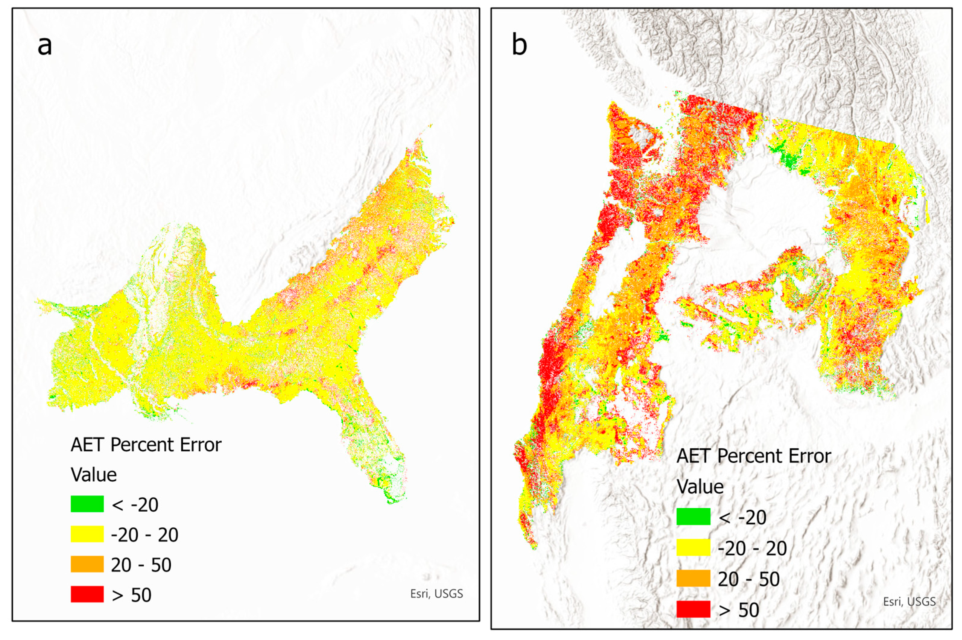
2.2. Model Validation
2.3. Hotspot and Coldspot Analysis
3. Results
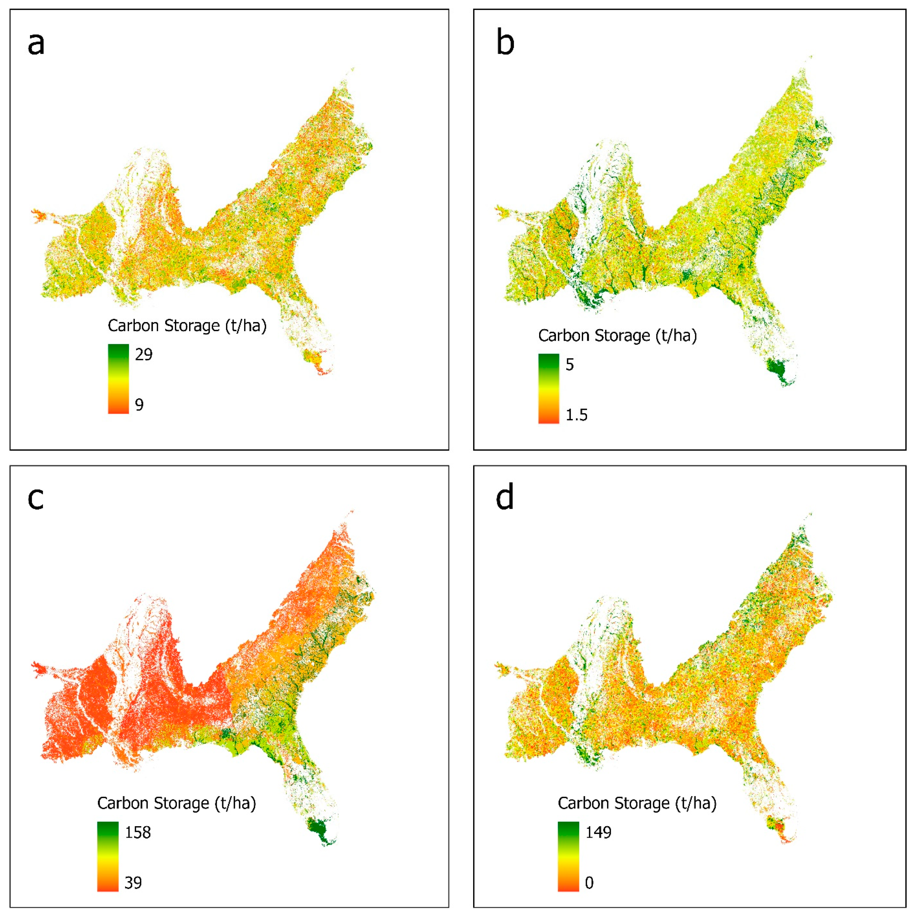
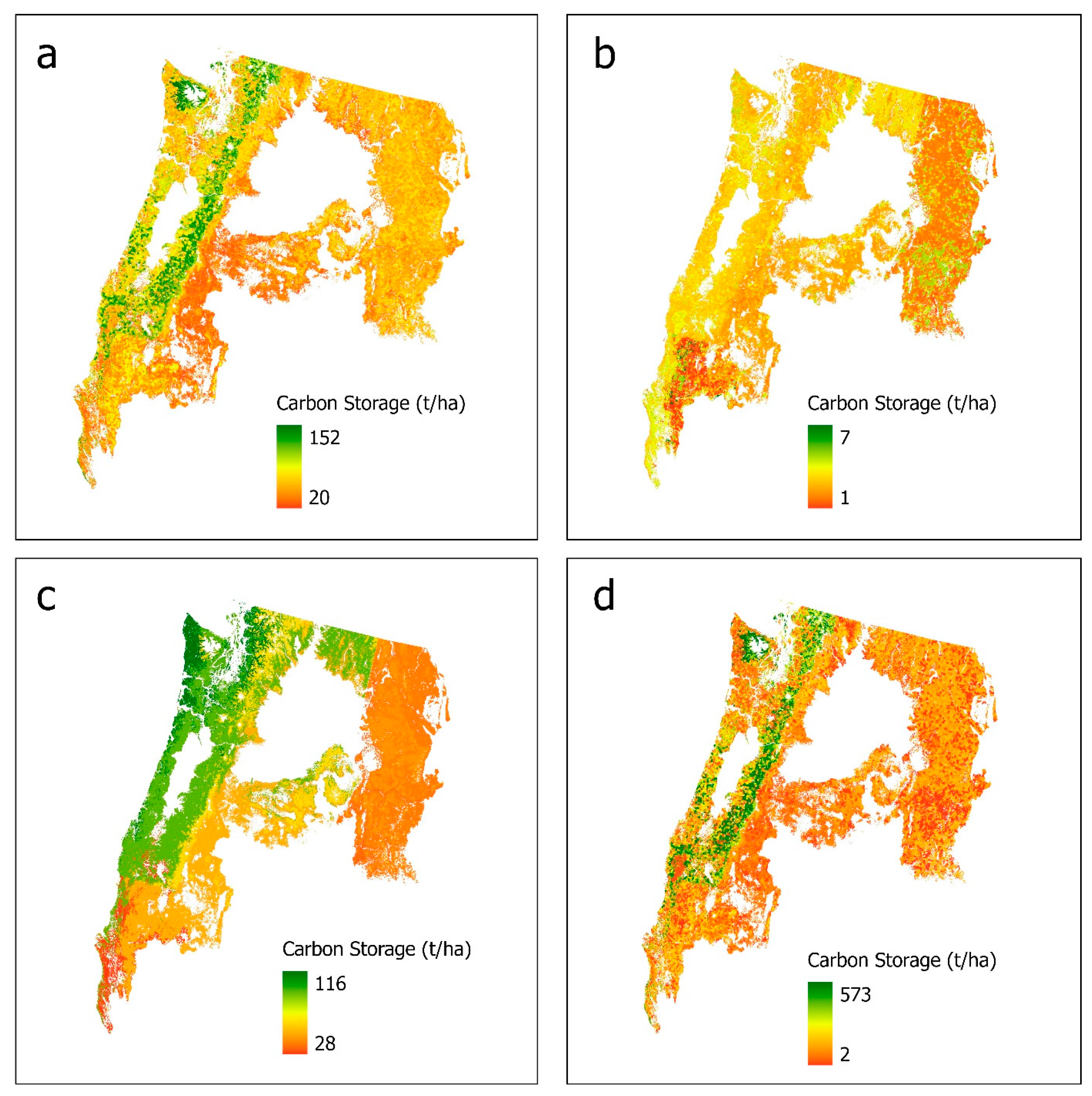
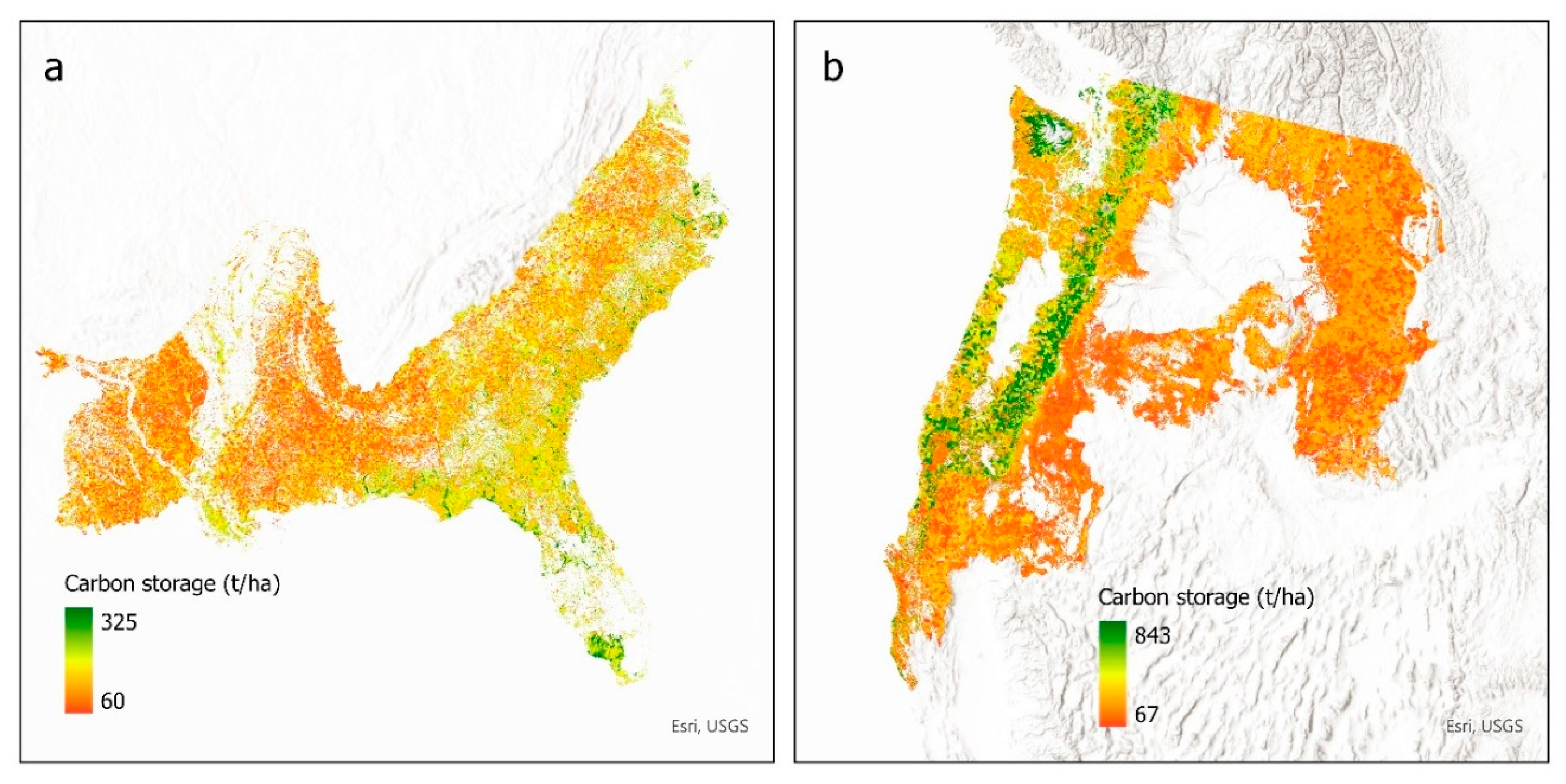
3.1. Carbon Storage
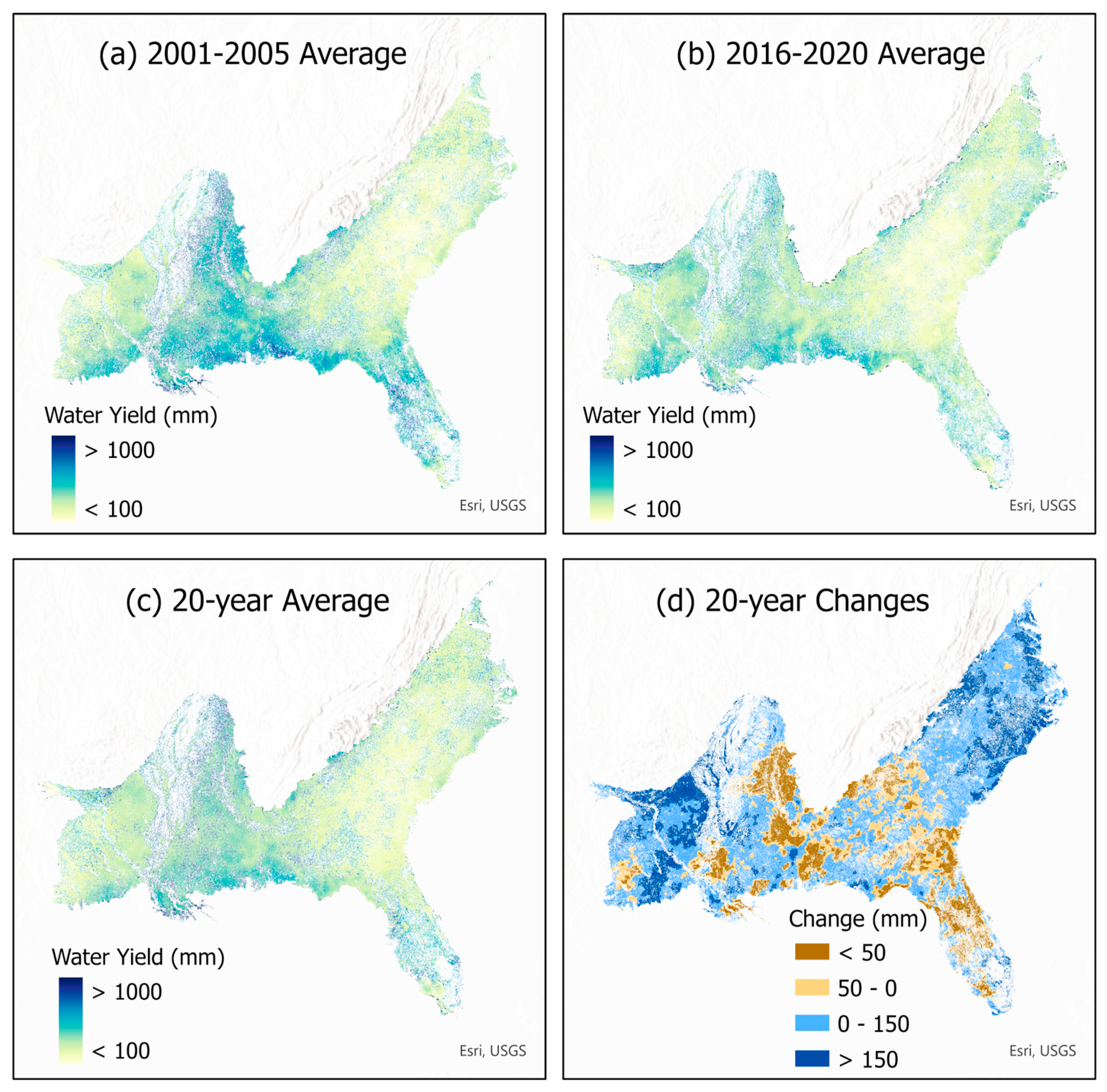
3.2. Water Yield
3.3. Hotspot Zones
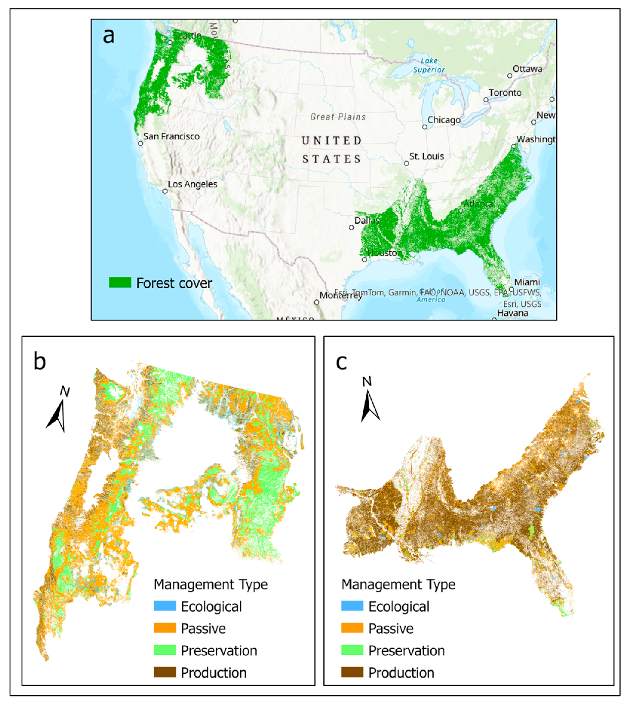
3.4. Management Types
4. Discussion
4.1. Carbon Storage
4.2. Water Yield
4.3. Hotspots and Coldspots
4.4. Management Types
4.5. Implications for Forest Management and Planning
4.6. Limitations and Future Research
5. Conclusions
Author Contributions
Funding
Data Availability Statement
Conflicts of Interest
Abbreviations
| InVEST | Integrated Valuation of Ecosystem Services and Tradeoffs |
| SEUS | Southeast United States |
| PNW | Pacific Northwest |
| DEM | Digital Elevation Model |
| U.S. | United States of America |
Appendix A. Maps of Carbon Storage Pools in the SEUS and PNW Regions
Appendix B. Water Yield Model Equations and Parameters
Appendix C. Validation of InVEST-Modeled AET Against Modis-Based Observations in the SEUS and PNW
References
- Mori, A. Biodiversity and ecosystem services in forests: Management and restoration founded on ecological theory. J. Appl. Ecol. 2017, 54, 7–11. [Google Scholar] [CrossRef]
- Triviño, M.; Juutinen, A.; Mazziotta, A.; Miettinen, K.; Podkopaev, D.; Reunanen, P.; Mönkkönen, M. Managing a boreal forest landscape for providing timber, storing and sequestering carbon. Ecosyst. Serv. 2015, 14, 179–189. [Google Scholar] [CrossRef]
- Pan, Y.; Birdsey, R.A.; Fang, J.; Houghton, R.; Kauppi, P.E.; Kurz, W.A.; Phillips, O.L.; Shvidenko, A.; Lewis, S.L.; Canadell, J.G.; et al. A large and persistent carbon sink in the world’s forests. Science 2011, 313, 988–993. [Google Scholar] [CrossRef]
- Friedlingstein, P.; O’Sullivan, M.; Jones, M.W.; Andrew, R.M.; Gregor, L.; Hauck, J.; Le Quéré, C.; Luijkx, I.T.; Olsen, A.; Peters, G.P.; et al. Global Carbon Budget 2022. Earth Syst. Sci. Data 2022, 14, 4811–4900. [Google Scholar] [CrossRef]
- Brown, T.C.; Hobbins, M.T.; Ramirez, J.A. Spatial distribution of water supply in the coterminous United States 1. JAWRA J. Am. Water Resour. Assoc. 2008, 44, 1474–1487. [Google Scholar] [CrossRef]
- Caldwell, P.V.; Martin, K.L.; Vose, J.M.; Baker, J.S.; Warziniack, T.W.; Costanza, J.K.; Frey, G.E.; Nehra, A.; Mihiar, C.M. Forested watersheds provide the highest water quality among all land cover types, but the benefit of this ecosystem service depends on landscape context. Sci. Total Environ. 2023, 882, 163550. [Google Scholar] [CrossRef]
- Zhang, M.; Wei, X. Deforestation, forestation, and water supply. Science 2021, 371, 990–991. [Google Scholar] [CrossRef]
- Liu, N.; Caldwell, P.V.; Dobbs, G.R.; Miniat, C.F.; Bolstad, P.V.; Nelson, S.A.C.; Sun, G. Forested lands dominate drinking water supply in the conterminous United States. Environ. Res. Lett. 2021, 16, 084008. [Google Scholar] [CrossRef]
- Anderegg, W.R.L.; Trugman, A.T.; Badgley, G.; Anderson, C.M.; Bartuska, A.; Ciais, P.; Cullenward, D.; Field, C.B.; Freeman, J.; Goetz, S.J.; et al. Climate-driven risks to the climate mitigation potential of forests. Science 2020, 368, eaaz7005. [Google Scholar] [CrossRef]
- Lipton, D.; Rubenstein, M.A.; Weiskopf, S.R.; Carter, S.L.; Peterson, J.; Crozier, L.; Fogarty, M.; Gaichas, S.; Hyde, K.J.; Morelli, T.L. Ecosystems, Ecosystem Services, and Biodiversity. Fourth Natl. Clim. Assess. 2018, 2, 268–321. [Google Scholar]
- Kleindl, W.; Rains, M.C.; Marshall, L.; Hauer, F. Fire and flood expand the floodplain shifting habitat mosaic concept. Freshw. Sci. 2015, 34, 1366–1382. [Google Scholar] [CrossRef]
- Weiskopf, S.R.; Rubenstein, M.A.; Crozier, L.G.; Gaichas, S.; Griffis, R.; Halofsky, J.E.; Hyde, K.J.W.; Morelli, T.L.; Morisette, J.T.; Muñoz, R.C.; et al. Climate change effects on biodiversity, ecosystems, ecosystem services, and natural resource management in the United States. Sci. Total Environ. 2020, 733, 137782. [Google Scholar] [CrossRef] [PubMed]
- Chang, H.; Bonnette, M.R. Climate change and water-related ecosystem services: Impacts of drought in california, USA. Ecosyst. Health Sustain. 2016, 2, e01254. [Google Scholar] [CrossRef]
- Balist, J.; Malekmohammadi, B.; Jafari, H.R.; Nohegar, A.; Geneletti, D. Detecting land use and climate impacts on water yield ecosystem service in arid and semi-arid areas. A study in Sirvan River Basin-Iran. Appl. Water Sci. 2021, 12, 4. [Google Scholar] [CrossRef]
- Bai, Y.; Ochuodho, T.O.; Yang, J. Impact of land use and climate change on water-related ecosystem services in Kentucky, USA. Ecol. Indic. 2019, 102, 51–64. [Google Scholar] [CrossRef]
- Pan, Q.; Wen, Z.; Wu, T.; Zheng, T.; Yang, Y.; Li, R.; Zheng, H. Trade-offs and synergies of forest ecosystem services from the perspective of plant functional traits: A systematic review. Ecosyst. Serv. 2022, 58, 101484. [Google Scholar] [CrossRef]
- Raudsepp-Hearne, C.; Peterson, G.D.; Bennett, E.M. Ecosystem service bundles for analyzing tradeoffs in diverse landscapes. Proc. Natl. Acad. Sci. USA 2010, 107, 5242–5247. [Google Scholar] [CrossRef]
- Orsi, F.; Ciolli, M.; Primmer, E.; Varumo, L.; Geneletti, D. Mapping hotspots and bundles of forest ecosystem services across the European Union. Land Use Policy 2020, 99, 104840. [Google Scholar] [CrossRef]
- Clarke, N.; Gundersen, P.; Jönsson-Belyazid, U.; Kjønaas, O.J.; Persson, T.; Sigurdsson, B.D.; Stupak, I.; Vesterdal, L. Influence of different tree-harvesting intensities on forest soil carbon stocks in boreal and northern temperate forest ecosystems. For. Ecol. Manag. 2015, 351, 9–19. [Google Scholar] [CrossRef]
- Mayer, M.; Prescott, C.E.; Abaker, W.E.A.; Augusto, L.; Cécillon, L.; Ferreira, G.W.D.; James, J.; Jandl, R.; Katzensteiner, K.; Laclau, J.-P.; et al. Tamm Review: Influence of forest management activities on soil organic carbon stocks: A knowledge synthesis. For. Ecol. Manag. 2020, 466, 118127. [Google Scholar] [CrossRef]
- del Campo, A.D.; Otsuki, K.; Serengil, Y.; Blanco, J.A.; Yousefpour, R.; Wei, X. A global synthesis on the effects of thinning on hydrological processes: Implications for forest management. For. Ecol. Manag. 2022, 519, 120324. [Google Scholar] [CrossRef]
- Duncker, P.S.; Raulund-Rasmussen, K.; Gundersen, P.; Katzensteiner, K.; De Jong, J.; Ravn, H.P.; Smith, M.; Eckmüllner, O.; Spiecker, H. How forest management affects ecosystem services, including timber production and economic return: Synergies and trade-offs. Ecol. Soc. 2012, 17, 50. [Google Scholar] [CrossRef]
- Chen, L.; Pei, S.; Liu, X.; Qiao, Q.; Liu, C. Mapping and analysing tradeoffs, synergies and losses among multiple ecosystem services across a transitional area in Beijing, China. Ecol. Indic. 2021, 123, 107329. [Google Scholar] [CrossRef]
- Tian, Z.; Upchurch, J.; Simon, G.A.; Dubeux, J.; Zare, A.; Zhao, C.; Harley, J.B. Quantifying Heterogeneous Ecosystem Services with Multi-Label Soft Classification. In Proceedings of the IGARSS 2024-2024 IEEE International Geoscience and Remote Sensing Symposium, Athens, Greece, 7–12 July 2024; pp. 427–431. [Google Scholar]
- Nelson, E.; Mendoza, G.; Regetz, J.; Polasky, S.; Tallis, H.; Cameron, D.; Chan, K.M.; Daily, G.C.; Goldstein, J.; Kareiva, P.M. Modeling multiple ecosystem services, biodiversity conservation, commodity production, and tradeoffs at landscape scales. Front. Ecol. Environ. 2009, 7, 4–11. [Google Scholar] [CrossRef]
- Hamel, P.; Guswa, A.J. Uncertainty analysis of a spatially explicit annual water-balance model: Case study of the Cape Fear basin, North Carolina. Hydrol. Earth Syst. Sci. 2015, 19, 839–853. [Google Scholar] [CrossRef]
- Heffernan, J.B.; Soranno, P.A.; Angilletta, M.J., Jr.; Buckley, L.B.; Gruner, D.S.; Keitt, T.H.; Kellner, J.R.; Kominoski, J.S.; Rocha, A.V.; Xiao, J. Macrosystems ecology: Understanding ecological patterns and processes at continental scales. Front. Ecol. Environ. 2014, 12, 5–14. [Google Scholar] [CrossRef]
- Kleindl, W.; Stoy, P.; Binford, M.; Desai, A.; Dietze, M.; Schultz, C.; Starr, G.; Staudhammer, C.; Wood, D. Toward a social-ecological theory of forest macrosystems for improved ecosystem management. Forests 2018, 9, 200. [Google Scholar] [CrossRef]
- Oswalt, S.N.; Smith, W.B.; Miles, P.D.; Pugh, S.A. Forest Resources of the United States, 2017: A Technical Document Supporting the Forest Service 2020 RPA Assessment; U.S. Department of Agriculture, Forest Service: Washington, DC, USA, 2019. [Google Scholar]
- Marsik, M.; Staub, C.G.; Kleindl, W.J.; Hall, J.M.; Fu, C.-S.; Yang, D.; Stevens, F.R.; Binford, M.W. Regional-scale management maps for forested areas of the Southeastern United States and the US Pacific Northwest. Sci. Data 2018, 5, 180165. [Google Scholar] [CrossRef] [PubMed]
- Felipe-Lucia, M.R.; Soliveres, S.; Penone, C.; Manning, P.; van der Plas, F.; Boch, S.; Prati, D.; Ammer, C.; Schall, P.; Gossner, M.M.; et al. Multiple forest attributes underpin the supply of multiple ecosystem services. Nat. Commun. 2018, 9, 4839. [Google Scholar] [CrossRef] [PubMed]
- Mitchell, R.J.; Liu, Y.; O’Brien, J.J.; Elliott, K.J.; Starr, G.; Miniat, C.F.; Hiers, J.K. Future climate and fire interactions in the southeastern region of the United States. For. Ecol. Manag. 2014, 327, 316–326. [Google Scholar] [CrossRef]
- Soil Survey Staff, Natural Resources Conservation Service, United States Department of Agriculture. Web Soil Survey. Available online: https://www.nrcs.usda.gov/ (accessed on 1 October 2024).
- Wear, D.N.; Greis, J.G. The southern forest futures project: Technical report. In Gen. Tech. Rep. SRS-GTR-178; USDA-Forest Service, Southern Research Station: Asheville, NC, USA, 2013; Volume 178, 542p. [Google Scholar] [CrossRef]
- PRISM Group, Oregon State University. Available online: https://prism.oregonstate.edu (accessed on 1 October 2024).
- U.S. Customs and Border Protection. Programmatic Environmental Impact Statement for Northern Border Activities: Appendix N—Geology, Topography, and Soils; U.S. Department of Homeland Security: Washington, DC, USA, 2012. [Google Scholar]
- Franklin, J.F.; Johnson, K.N. A restoration framework for federal forests in the Pacific Northwest. J. For. 2012, 110, 429–439. [Google Scholar] [CrossRef]
- Sharp, R.; Douglass, J.; Wolny, S.; Arkema, K.; Bernhardt, J.; Bierbower, W.; Chaumont, N.; Denu, D.; Fisher, D.; Glowinski, K. InVEST 3.8.7. User’s Guide. In The Natural Capital Project. 2020. Available online: https://invest.readthedocs.io/en/3.8.7/installing.html (accessed on 1 October 2024).
- Nelson, E.J.; Kareiva, P.; Ruckelshaus, M.; Arkema, K.; Geller, G.; Girvetz, E.; Goodrich, D.; Matzek, V.; Pinsky, M.; Reid, W. Climate change’s impact on key ecosystem services and the human well-being they support in the US. Front. Ecol. Environ. 2013, 11, 483–893. [Google Scholar] [CrossRef]
- Polasky, S.; Nelson, E.; Pennington, D.; Johnson, K.A. The impact of land-use change on ecosystem services, biodiversity and returns to landowners: A case study in the state of Minnesota. Environ. Resour. Econ. 2011, 48, 219–242. [Google Scholar] [CrossRef]
- Ruefenacht, B.; Finco, M.; Nelson, M.; Czaplewski, R.; Helmer, E.; Blackard, J.; Holden, G.; Lister, A.; Salajanu, D.; Weyermann, D. Conterminous US and Alaska forest type mapping using forest inventory and analysis data. Photogramm. Eng. Remote Sens. 2008, 74, 1379–1388. [Google Scholar] [CrossRef]
- Pan, Y.; Chen, J.M.; Birdsey, R.; McCullough, K.; He, L.; Deng, F. NACP Forest Age Maps at 1-km Resolution for Canada (2004) and the U.S.A. (2006); NASA: Washington, DC, USA, 2012. [Google Scholar] [CrossRef]
- Abatzoglou, J.T. Development of gridded surface meteorological data for ecological applications and modelling. Int. J. Climatol. 2013, 33, 121–131. [Google Scholar] [CrossRef]
- Allen, R.G.; Pereira, L.S.; Raes, D.; Smith, M. Crop evapotranspiration-Guidelines for computing crop water requirements-FAO Irrigation and drainage paper 56. FAO Rome 1998, 300, D05109. [Google Scholar]
- Schenk, H.J.; Jackson, R.B. Rooting depths, lateral root spreads and below-ground/above-ground allometries of plants in water-limited ecosystems. J. Ecol. 2002, 90, 480–494. [Google Scholar] [CrossRef]
- Yin, G.; Wang, X.; Zhang, X.; Fu, Y.; Hao, F.; Hu, Q. InVEST model-based estimation of water yield in North China and its sensitivities to climate variables. Water 2020, 12, 1692. [Google Scholar] [CrossRef]
- Senay, G.B.; Kagone, S.; Velpuri, N.M. Operational Global Actual Evapotranspiration: Development, Evaluation and Dissemination. Sensors 2020, 20, 1915. [Google Scholar] [CrossRef] [PubMed]
- Li, Y.; Zhang, L.; Yan, J.; Wang, P.; Hu, N.; Cheng, W.; Fu, B. Mapping the hotspots and coldspots of ecosystem services in conservation priority setting. J. Geogr. Sci. 2017, 27, 681–696. [Google Scholar] [CrossRef]
- Karimi, H.; Binford, M.; Kleindl, W.; Starr, G.; Murphy, B.A.; Desai, A.R.; Fu, C.S.; Dietze, M.C.; Staudhammer, C. Drivers of forest productivity in two regions of the United States: Relative impacts of management and environmental variables. J. Environ. Manag. 2025, 374, 124040. [Google Scholar] [CrossRef]
- Egoh, B.; Reyers, B.; Rouget, M.; Richardson, D.M.; Le Maitre, D.C.; van Jaarsveld, A.S. Mapping ecosystem services for planning and management. Agric. Ecosyst. Environ. 2008, 127, 135–140. [Google Scholar] [CrossRef]
- Case, M.J.; Johnson, B.G.; Bartowitz, K.J.; Hudiburg, T.W. Forests of the future: Climate change impacts and implications for carbon storage in the Pacific Northwest, USA. For. Ecol. Manag. 2021, 482, 118886. [Google Scholar] [CrossRef]
- Dilustro, J.J.; Collins, B.; Duncan, L.; Crawford, C. Moisture and soil texture effects on soil CO2 efflux components in southeastern mixed pine forests. For. Ecol. Manag. 2005, 204, 87–97. [Google Scholar] [CrossRef]
- Garten, C.T.; Hanson, P.J. Measured forest soil C stocks and estimated turnover times along an elevation gradient. Geoderma 2006, 136, 342–352. [Google Scholar] [CrossRef]
- Nave, L.E.; DeLyser, K.; Domke, G.M.; Holub, S.M.; Janowiak, M.K.; Ontl, T.A.; Sprague, E.; Viau, N.R.; Walters, B.F.; Swanston, C.W. Soil carbon in the South Atlantic United States: Land use change, forest management, and physiographic context. For. Ecol. Manag. 2022, 520, 120410. [Google Scholar] [CrossRef]
- Napton, D.E.; Auch, R.F.; Headley, R.; Taylor, J.L. Land changes and their driving forces in the Southeastern United States. Reg. Environ. Change 2010, 10, 37–53. [Google Scholar] [CrossRef]
- James, J.; Harrison, R. The effect of harvest on forest soil carbon: A meta-analysis. Forests 2016, 7, 308. [Google Scholar] [CrossRef]
- Fagan, M.; Morton, D.; Cook, B.; Masek, J.; Zhao, F.; Nelson, R.; Huang, C. Mapping pine plantations in the southeastern US using structural, spectral, and temporal remote sensing data. Remote Sens. Environ. 2018, 216, 415–426. [Google Scholar] [CrossRef]
- Birdsey, R.A.; DellaSala, D.A.; Walker, W.S.; Gorelik, S.R.; Rose, G.; Ramírez, C.E. Assessing carbon stocks and accumulation potential of mature forests and larger trees in US federal lands. Front. For. Glob. Change 2023, 5, 1074508. [Google Scholar] [CrossRef]
- Siler, N.; Roe, G.; Durran, D. On the dynamical causes of variability in the rain-shadow effect: A case study of the Washington Cascades. J. Hydrometeorol. 2013, 14, 122–139. [Google Scholar] [CrossRef]
- Siler, N.; Durran, D. What causes weak orographic rain shadows? Insights from case studies in the Cascades and idealized simulations. J. Atmos. Sci. 2016, 73, 4077–4099. [Google Scholar] [CrossRef]
- Bohne, L.; Strong, C.; Steenburgh, W.J. Climatology of orographic precipitation gradients in the contiguous western united states. J. Hydrometeorol. 2020, 21, 1723–1740. [Google Scholar] [CrossRef]
- Smith, W.B.; Miles, P.D.; Perry, C.H.; Pugh, S.A. Forest Resources of the United States, 2007; U.S. Department of Agriculture, Forest Service, Washington Office: Washington, DC, USA, 2017. [Google Scholar] [CrossRef]
- Hoover, C.M.; Bagdon, B.; Gagnon, A. Standard Estimates of Forest Ecosystem Carbon for Forest Types of the United States; U.S. Department of Agriculture, Forest Service, Northern Research Station: Madison, WI, USA, 2021. [Google Scholar]
- Luyssaert, S.; Schulze, E.D.; Borner, A.; Knohl, A.; Hessenmoller, D.; Law, B.E.; Ciais, P.; Grace, J. Old-growth forests as global carbon sinks. Nature 2008, 455, 213–215. [Google Scholar] [CrossRef]
- Sun, G.; McNulty, S.G.; Lu, J.; Amatya, D.M.; Liang, Y.; Kolka, R. Regional annual water yield from forest lands and its response to potential deforestation across the southeastern United States. J. Hydrol. 2005, 308, 258–268. [Google Scholar] [CrossRef]
- Acharya, S.; Kaplan, D.A.; McLaughlin, D.L.; Cohen, M.J. In-situ quantification and prediction of water yield from southern US pine forests. Water Resour. Res. 2022, 58, e2021WR031020. [Google Scholar] [CrossRef]
- Tague, C.; Grant, G.; Farrell, M.; Choate, J.; Jefferson, A. Deep groundwater mediates streamflow response to climate warming in the Oregon Cascades. Clim. Change 2008, 86, 189–210. [Google Scholar] [CrossRef]
- Perry, T.D.; Jones, J.A. Summer streamflow deficits from regenerating Douglas-fir forest in the Pacific Northwest, USA. Ecohydrology 2017, 10, e1790. [Google Scholar] [CrossRef]
- Duarte, H.F.; Kim, J.B.; Sun, G.; McNulty, S.G.; Xiao, J. Climate and vegetation change impacts on future conterminous United States water yield. J. Hydrol. 2024, 639, 131472. [Google Scholar] [CrossRef]
- Liu, M.; Adam, J.C.; Hamlet, A.F. Spatial-temporal variations of evapotranspiration and runoff/precipitation ratios responding to the changing climate in the Pacific Northwest during 1921–2006. J. Geophys. Res. Atmos. 2013, 118, 380–394. [Google Scholar] [CrossRef]
- Sun, G.; Caldwell, P.V.; McNulty, S.G. Modelling the potential role of forest thinning in maintaining water supplies under a changing climate across the conterminous United States. Hydrol. Process. 2015, 29, 5016–5030. [Google Scholar] [CrossRef]
- Jackson, R.B.; Jobbagy, E.G.; Avissar, R.; Roy, S.B.; Barrett, D.J.; Cook, C.W.; Farley, K.A.; le Maitre, D.C.; McCarl, B.A.; Murray, B.C. Trading water for carbon with biological carbon sequestration. Science 2005, 310, 1944–1947. [Google Scholar] [CrossRef]
- Trabucco, A.; Zomer, R.J.; Bossio, D.A.; van Straaten, O.; Verchot, L.V. Climate change mitigation through afforestation/reforestation: A global analysis of hydrologic impacts with four case studies. Agric. Ecosyst. Environ. 2008, 126, 81–97. [Google Scholar] [CrossRef]
- Pisarello, K.L.; Sun, G.; Evans, J.M.; Fletcher, R.J. Potential long term water yield impacts from pine plantation management strategies in the southeastern United States. For. Ecol. Manag. 2022, 522, 120454. [Google Scholar] [CrossRef]
- Becknell, J.M.; Desai, A.R.; Dietze, M.C.; Schultz, C.A.; Starr, G.; Duffy, P.A.; Franklin, J.F.; Pourmokhtarian, A.; Hall, J.; Stoy, P.C. Assessing interactions among changing climate, management, and disturbance in forests: A macrosystems approach. BioScience 2015, 65, 263–274. [Google Scholar] [CrossRef]
- Hodder, K.H.; Newton, A.C.; Cantarello, E.; Perrella, L. Does landscape-scale conservation management enhance the provision of ecosystem services? Int. J. Biodivers. Sci. Ecosyst. Serv. Manag. 2014, 10, 71–83. [Google Scholar] [CrossRef]
- Sun, G.; Zhang, L.; Duan, K.; Rau, B.; Efroymson, R.; Langholtz, M.; Johnson, K.; Stokes, B. Impacts of forest biomass removal on water yield across the United States, Chapter 7 (Eds.). In Billion-Ton Report: Advancing Domestic Resources for a Thriving Bioeconomy; Oak Ridge National Laboratory: Oak Ridge, TN, USA, 2017. [Google Scholar] [CrossRef]
- Christopher, S.F.; Schoenholtz, S.H.; Nettles, J.E. Water quantity implications of regional-scale switchgrass production in the southeastern US. Biomass Bioenergy 2015, 83, 50–59. [Google Scholar] [CrossRef]
- Hernandez, R.C.; Camerin, F. The application of ecosystem assessments in land use planning: A case study for supporting decisions toward ecosystem protection. Futures 2024, 161, 103399. [Google Scholar] [CrossRef]
- Pilogallo, A.; Saganeiti, L.; Scorza, F.; Murgante, B. Assessing the impact of land use changes on ecosystem services value. In Proceedings of the International Conference on Computational Science and Its Applications, Istanbul, Türkiye, 30 June–3 July 2020; pp. 606–616. [Google Scholar]
- Lv, G.; Wang, Y.; Ma, X.; Han, Y.; Luo, C.; Yu, W.; Liu, J.; Du, Z. Trade-Offs and Synergies of Ecosystem Services in Terminal Lake Basins of Arid Regions Under Environmental Change: A Case Study of the Ebinur Lake Basin. Land 2025, 14, 1240. [Google Scholar] [CrossRef]
- Hoover, C.M.; Smith, J.E. Aboveground live tree carbon stock and change in forests of conterminous United States: Influence of stand age. Carbon Balance Manag. 2023, 18, 7. [Google Scholar] [CrossRef]
- Gray, A.N.; Whittier, T.R.; Harmon, M.E. Carbon stocks and accumulation rates in Pacific Northwest forests: Role of stand age, plant community, and productivity. Ecosphere 2016, 7, e01224. [Google Scholar] [CrossRef]
- Hamel, P.; Valencia, J.; Schmitt, R.; Shrestha, M.; Piman, T.; Sharp, R.P.; Francesconi, W.; Guswa, A.J. Modeling seasonal water yield for landscape management: Applications in Peru and Myanmar. J. Environ. Manag. 2020, 270, 110792. [Google Scholar] [CrossRef] [PubMed]
- Zhang, L.; Dawes, W.; Walker, G. Response of mean annual evapotranspiration to vegetation changes at catchment scale. Water Resour. Res. 2001, 37, 701–708. [Google Scholar] [CrossRef]


| Data | Source | Resolution |
|---|---|---|
| Stand age | [42] | 250 m |
| Forest type groups | US Forest Service | 250 m |
| Precipitation | PRISM | 4 km |
| Reference ET | [43] | 1 km |
| Root restricting layer depth | SSURGO | 30 m |
| Plant available water content | SSURGO | 30 m |
| Land use/cover | NLCD | 30 m |
| Biophysical variables (CN, Kc, etc.) | Literature/InVEST documentation | - |
| % Regional Area | |||
|---|---|---|---|
| Management Type | The Primary Goal of Management | SEUS | PNW |
| Production | To extract wood products for economic gain. | 67 | 10 |
| Preservation | To promote ecological diversity by minimizing human consumptive services and maximizing other ecosystem services. | 4 | 27 |
| Ecological | To balance wood product extraction with the maintenance of other ecosystem services. | 1 | 12 |
| Passive | Rather than a goal, forests are primarily left alone—too wet to harvest or to protect sensitive species (riparian areas)—or owned by people who enjoy their aesthetics or simply neglected. | 28 | 51 |
| Forest Type Group | Area (%) | Mean (t ha−1) | Standard Deviation | Sum (MT) | Sum (%) |
|---|---|---|---|---|---|
| Loblolly/Shortleaf Pine | 41.65 | 130.6 | 41.1 | 3451.9 | 35.74 |
| Oak/Gum/Cypress | 16.41 | 189.0 | 64.5 | 1964.4 | 20.34 |
| Oak/Hickory | 23.60 | 127.6 | 46.4 | 1924.4 | 19.93 |
| Longleaf/Slash Pine | 9.38 | 175.5 | 39.0 | 1318.1 | 13.65 |
| Oak/Pine | 7.64 | 133.1 | 44.0 | 730.6 | 7.56 |
| Elm/Ash/Cottonwood | 1.29 | 154.8 | 47.1 | 164.4 | 1.70 |
| Other Eastern groups | 0.03 | 154.8 | 45.2 | 23.1 | 0.24 |
| Forest Type Group | Area (%) | Mean (t ha−1) | Standard Deviation | Sum (MT) | Sum (%) |
|---|---|---|---|---|---|
| Douglas Fir | 42.29 | 353.7 | 202.1 | 5530.0 | 52.30 |
| Fir/Spruce/Mountain Hemlock | 19.87 | 265.5 | 128.8 | 1938.8 | 18.34 |
| Ponderosa Pine | 13.95 | 148.0 | 39.0 | 751.3 | 7.10 |
| Hemlock/Sitka Spruce | 4.64 | 408.3 | 242.1 | 698.1 | 6.60 |
| California Mixed Conifer | 6.01 | 224.7 | 83.9 | 500.0 | 4.73 |
| Lodgepole Pine | 4.42 | 158.9 | 55.1 | 257.5 | 2.44 |
| Alder/Maple | 2.06 | 335.8 | 140.5 | 255.0 | 2.41 |
| Tanoak/Laurel | 1.88 | 213.7 | 139.0 | 148.1 | 1.40 |
| Western Oak | 1.80 | 207.9 | 74.0 | 137.5 | 1.30 |
| Pinyon/Juniper | 2.21 | 154.7 | 31.4 | 124.4 | 1.18 |
| Redwood | 0.64 | 478.3 | 185.1 | 113.1 | 1.07 |
| Other Western groups | 0.22 | 238.6 | 90.1 | 92.5 | 1.13 |
| Region | Management Type | Correlation Coefficient |
|---|---|---|
| SEUS | Ecological | −0.075 |
| Passive | −0.019 | |
| Preservation | −0.042 | |
| Production | −0.074 | |
| Overall | −0.042 | |
| PNW | Ecological | 0.341 |
| Passive | 0.396 | |
| Preservation | 0.590 | |
| Production | 0.223 | |
| Overall | 0.437 |
| Region | Management Type | % Regional Area | Proportion of Regional Carbon Hotspots | Ratio (Carbon Hotspot–Area) | Proportion of Regional Water Yield Hotspots | Ratio (Water Hotspot–Area) |
|---|---|---|---|---|---|---|
| SEUS | Ecological | 1 | 4 | 4 | 2 | 2 |
| Passive | 28 | 32 | 1.1 | 32 | 1.1 | |
| Preservation | 4 | 10 | 2.1 | 4 | 1.0 | |
| Production | 67 | 54 | 0.8 | 62 | 0.9 | |
| PNW | Ecological | 12 | 8 | 0.6 | 10 | 0.8 |
| Passive | 51 | 53 | 1.0 | 45 | 0.9 | |
| Preservation | 27 | 27 | 1.0 | 28 | 1.0. | |
| Production | 10 | 12 | 1.3 | 17 | 1.7 |
Disclaimer/Publisher’s Note: The statements, opinions and data contained in all publications are solely those of the individual author(s) and contributor(s) and not of MDPI and/or the editor(s). MDPI and/or the editor(s) disclaim responsibility for any injury to people or property resulting from any ideas, methods, instructions or products referred to in the content. |
© 2025 by the authors. Licensee MDPI, Basel, Switzerland. This article is an open access article distributed under the terms and conditions of the Creative Commons Attribution (CC BY) license (https://creativecommons.org/licenses/by/4.0/).
Share and Cite
Karimi, H.; Staudhammer, C.L.; Therrell, M.D.; Kleindl, W.J.; Mungai, L.M.; Amanambu, A.C.; Jones, C.N. Mapping Tradeoffs and Synergies in Ecosystem Services as a Function of Forest Management. Land 2025, 14, 1591. https://doi.org/10.3390/land14081591
Karimi H, Staudhammer CL, Therrell MD, Kleindl WJ, Mungai LM, Amanambu AC, Jones CN. Mapping Tradeoffs and Synergies in Ecosystem Services as a Function of Forest Management. Land. 2025; 14(8):1591. https://doi.org/10.3390/land14081591
Chicago/Turabian StyleKarimi, Hazhir, Christina L. Staudhammer, Matthew D. Therrell, William J. Kleindl, Leah M. Mungai, Amobichukwu C. Amanambu, and C. Nathan Jones. 2025. "Mapping Tradeoffs and Synergies in Ecosystem Services as a Function of Forest Management" Land 14, no. 8: 1591. https://doi.org/10.3390/land14081591
APA StyleKarimi, H., Staudhammer, C. L., Therrell, M. D., Kleindl, W. J., Mungai, L. M., Amanambu, A. C., & Jones, C. N. (2025). Mapping Tradeoffs and Synergies in Ecosystem Services as a Function of Forest Management. Land, 14(8), 1591. https://doi.org/10.3390/land14081591