Article

Integrating Remote Sensing, Landscape Metrics, and Random Forest Algorithm to Analyze Crop Patterns, Factors, Diversity, and Fragmentation in a Kharif Agricultural Landscape

by
Surajit Banerjee
1,
Tuhina Nandi
2,3,
Vishwambhar Prasad Sati
1,4,
Wiem Mezlini
5,
Wafa Saleh Alkhuraiji
6,
Djamil Al-Halbouni
7,* and
Mohamed Zhran
8,*
1
Department of Geography and Resources Management, Mizoram University, Aizawl 796004, India
2
Agricultural Insurance Company of India Limited, New Delhi 110023, India
3
Department of Geo-Informatics, Pandit Raghunath Murmu Smriti, Mahavidyalaya, Bankura University, Bankura 722155, India
4
Impact Policy Research Institute, New Delhi 110017, India
5
Department of Geology, Faculty of Sciences, University of Tunis El Manar, Tunis 2092, Tunisia
6
Department of Geography and Environmental Sustainability, College of Humanities and Social Sciences, Princess Nourah bint Abdulrahman University, P.O. BOX 84428, Riyadh 11671, Saudi Arabia
7
Institute for Earth System Science and Remote Sensing, University of Leipzig, 04103 Leipzig, Germany
8
Public Works Engineering Department, Faculty of Engineering, Mansoura University, Mansoura 35516, Egypt
*
Authors to whom correspondence should be addressed.
Land 2025, 14(6), 1203; https://doi.org/10.3390/land14061203
Submission received: 14 April 2025 / Revised: 19 May 2025 / Accepted: 27 May 2025 / Published: 4 June 2025
(This article belongs to the Special Issue Digital Earth and Remote Sensing for Land Management)

Abstract

Despite growing importance, agricultural landscapes face threats, like fragmentation, shrinkage, and degradation, due to climate change. Although remote sensing and GIS are widely used in monitoring croplands, integrating machine learning, remote sensing, GIS, and landscape metrics for the holistic management of this landscape remains underexplored. Thus, this study monitored crop patterns using random forest (94% accuracy), the role of geographical factors (such as elevation, aspect, slope, maximum and minimum temperature, rainfall, cation exchange capacity, NPK, soil pH, soil organic carbon, soil type, soil water content, proximity to drainage, proximity to market, proximity to road, population density, and profit per hectare production), diversity, combinations, and fragmentation using landscape metrics and a fragmentation index. Findings revealed that slope, rainfall, temperature, and profit per hectare production emerged as significant drivers in shaping crop patterns. However, anthropogenic drivers became deciding factors during spatial overlaps between crop suitability zones. Rice belts were the least fragmented and highly productive with a risk of monoculture. Croplands with a combination of soybean, black grams, and maize were highly fragmented, despite having high diversity with comparatively less production per field. These diverse fields were providing higher profits and low risks of crop failure due to the crop combinations. Equally, intercropping balanced the nutrient uptakes, making the practice sustainable. Thus, it can be suggested that productivity and diversity should be prioritized equally to achieve sustainable land use. The development of the PCA-weighted fragmentation index offers an efficient tool to measure fragmentation across similar agricultural regions, and the integrated approach provides a scalable framework for holistic management, sustainable land use planning, and precision agriculture.

1. Introduction

Agroecosystems and agricultural landscapes cover 37% of the total land area globally, of which 12% is under cropland. These croplands are crucial for global food security, billions of livelihoods, habitat protection, environmental processes regulation, and ecological balance maintenance. However, over the last two decades, cropland degradation has become a common issue attributed to desertification, soil erosion, fertility loss, and global land use alteration [1,2,3,4,5,6]. Monocropping, rainfed intensive farming, and the traditional farming practices of Southeast Asia are the most vulnerable farming systems toward climate change, due to higher dependency on monsoonal rainfall [7,8,9,10,11,12]. India, particularly the central highlands, is characterized with rainfed farming and smallholder famers, so crop diversity is crucial to counter climatic uncertainties and market disruptions [13]. Thus, a deep understanding of crop patterns, diversity, combinations, and fragmentation becomes increasingly essential in the Kharif season to manage productivity and ecological stability. In addition, exploring the role of environmental and anthropogenic factors in shaping crop patterns is required to identify the region-specific needs of cropland management and the spatial distribution of vulnerable areas [14].
Advancements in remote sensing in recent years have revolutionized agriculture monitoring, crop classification, and crop health monitoring at a large spatial scale. However, the integration of other techniques and indices, such as machine learning and landscape metrics, are required to quantify spatial heterogeneity, crop combinations, and fragmentation. Machine learning techniques, such as support vector machine (SVM), k-nearest neighbor (KNN), and random forest (RF) classifiers, can model and quantify crop patterns with high-resolution spatial data and higher accuracy of the model [15,16]. Compared to the widely used traditional methods, such as the maximum likelihood classifier (MLC) and conventional techniques, these algorithms demonstrated better results in modeling [17,18]. Among these models, most of the preexisting studies advocated for better precision of the random forest algorithm [19,20]. Moreover, the computation of feature importance in RF effectively measures the relative importance of the factors. Coupling this technique with landscape metrics for a more profound understanding of patch dominance, crop diversity, combinations, and fragmentation in the agricultural landscape presents a strong framework, offering new insights into ecological and economic sustainability. However, existing studies have not addressed this potential gap, leaving a remarkable gap in the holistic assessment of agricultural landscapes.
Previous research has focused on the identification of crop types based on supervised classification techniques, the comparison of the performance of different methods in crop classification, the integration of machine learning and remote sensing in precision agriculture, crop yield estimation, disease monitoring, and crop health monitoring [21,22,23,24,25]. Most existing studies have used traditional techniques to show crop combinations and diversity throughout a large region. However, the wide use of remote sensing and landscape metrics is rare [26].
Studies on fragmentation using landscape metrics are present in habitat studies, forest studies, land use and land cover, and vegetation studies; whereas, their usage in agriculture is limited [27,28,29,30]. Most of the fragmentation-related studies on cropland selected a single metric and developed fragmentation indices based on any of the mentioned aspects, such as areal division, temporal change over time, and morphological spatial pattern analysis [31,32,33,34]. A comprehensive fragmentation index covering all the aspects of fragmentation, such as shape complexity, areal change, patch dynamics, edge effects, clustering pattern, and splitting nature, is absent yet necessary. Therefore, this study has attempted to bridge these gaps by exploring the capacity of combining remote sensing, machine learning, and landscape metrics to study the landscape ecology of agricultural landscapes. The objectives of this research are (1) to identify crop patterns using machine learning during the Kharif season, (2) to assess the role of environmental and anthropogenic factors in shaping the pattern, (3) to evaluate diversity, dominance, combinations, and degree of fragmentation in cropping systems using class and landscape-level metrics, and (4) to develop a robust, scalable, and objectively weighted fragmentation index to assess the spatial structure of crop fields.

2. Materials and Methods
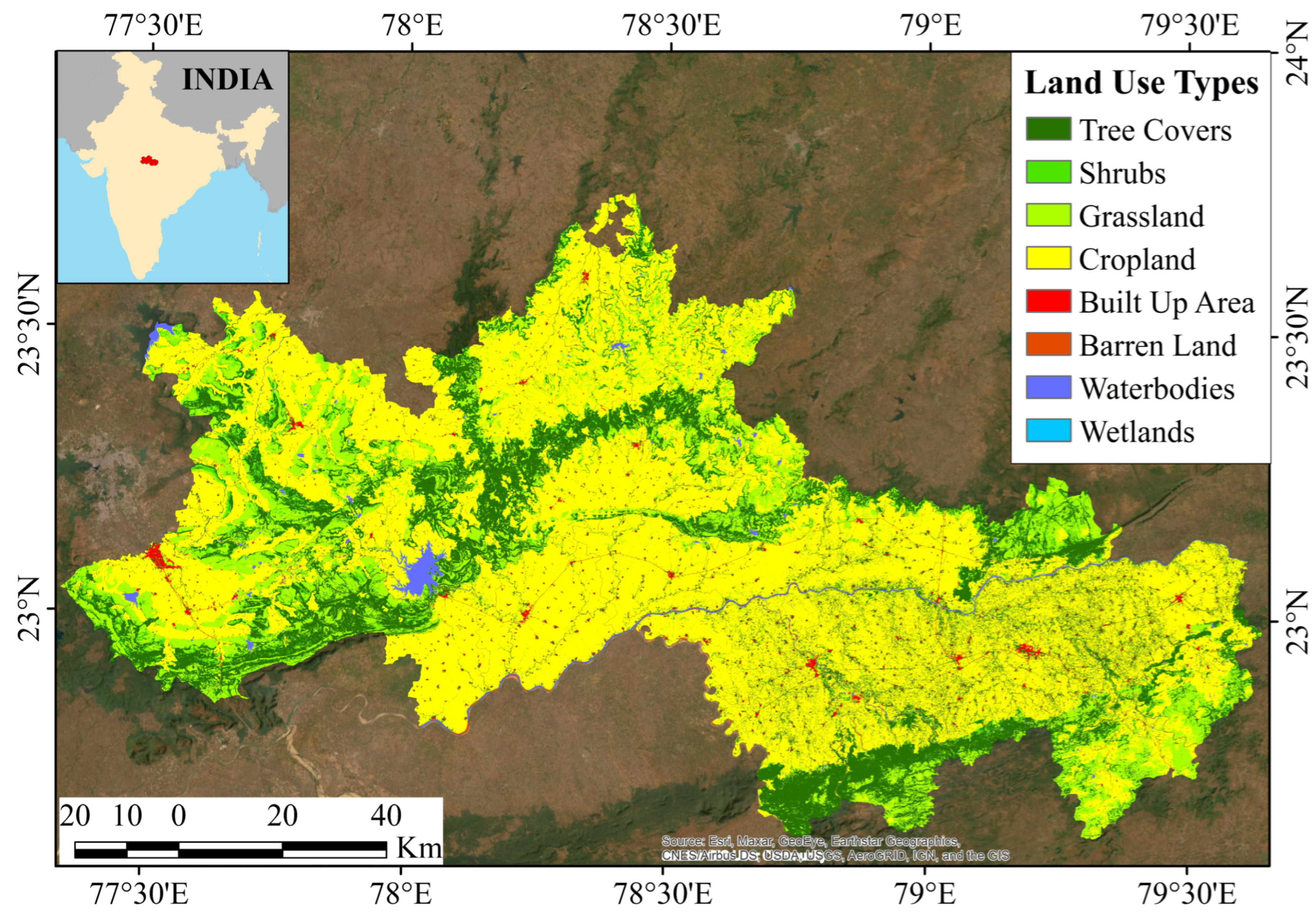
2.1. Study Area

Raisen and Narsinghpur are two districts with the most diverse topography and agro-ecological settings in the central Indian state of Madhya Pradesh. Their collective geographical area is 13,591 km2, extending from 77°18′ E to 79°42′ E and 22°36′ N to 24°06′ N (Figure 1).
The region’s diverse topography includes undulating rocky surfaces, hills, plateaus, deep river valleys, and expansive plains with a significant variation in relief, ranging from 300 m to 700 m. The most important river, the Narmada, flows westward, following the rift valley between the Vindhyan and Satpura ranges. Other significant rivers originating from these highlands include the Betwa, Tawa, Shakkar, and Dudhi [35]. Multiple small and medium-sized dams along these rivers fulfil the need for irrigation in the surrounding areas. The temperature in the Kharif season varies from 32 °C to 46 °C and in winter from 12 °C to 28 °C [36]. The annual average precipitation ranges between 800 mm and 1300 mm. The hot and semi-arid climate of the region supports dry deciduous forest of Sal (Shorea robusta), Teak (Tectona grandis), and Indian Ber (Ziziphus mauritiana), the shrublands of Acasia, and the thorny grassland types of natural vegetation [37]. The region consists of black regur soil (supports soybeans, wheat, cotton, and pulses), alluvial soils (ideal for rice and sugarcane), red soil, and laterite soil. During the Kharif season (June to October), the region typically supports the cultivation of soybean, rice, maize, black gram, and green gram. While in the Rabi season (winter), lentils, peas, chickpeas, and wheat are grown. The selected study area provides a wider platform to study these characteristics in a single region due to the presence of rainfed agriculture, irrigation-dependent agriculture, semi-arid croplands, and transition zones. The majority of Indian agricultural land has similar characteristics. Thus, the study area also emerges as representative of the entire landscape.

2.2. Methods

Figure 2 shows the flow of methodology applied to conduct the research applied to the study area.

2.2.1. Data Used

The normalized difference vegetation index (NDVI) was calculated based on red and NIR (near infrared) bands of Sentinel 2A, with 10 m resolution, obtained from the Copernicus image collections in the Google Earth Engine (GEE). In this study, NDVI was not solely used for the spectral discrimination; instead, a time series of NDVI was utilized to capture phenological dynamics of crops. Previous studies have shown that a multitemporal NDVI remains effective in crop-type mapping when combined with a machine learning-based classifier with a supervised approach based on ground crop-type data [38].
Crop-type data were collected from the field with their GPS location using a spatially stratified survey, ensuring comprehensive representation across all crop types and administrative blocks. Sample locations were taken based on the ground knowledge of the different crop types present in the fields. Twenty to thirty sample points covering major crop types from each administrative tehsil were recorded based on the size of the tehsil. Based on the proportion of crop types, samples were chosen proportionately, as mentioned in Table 1. As machine learning algorithms can experience overfitting and larger variance with lower number of samples, to counter this problem, a total of 500 samples were chosen [39]. Then, these points with 10 m buffers were used as training and testing data (70:30) to classify the crop types using a random forest algorithm.
The drivers of crop pattern data on climatic, topographic, edaphic, and anthropogenic determinants were collected. For instance, rainfall, maximum temperature, and minimum temperature were selected among climatic drivers. The respective data were collected with a 25 s spatial resolution from the WorldClim portal. Topographic drivers, such as elevation, slope, and aspect, were also incorporated from the shuttle radar topography mission (SRTM) digital elevation model (DEM) data, accessed via the United States Geological Survey (USGS) Earth Explorer platform. Edaphic drivers, such as data on soil pH, cation exchange capacity (CEC), soil type, NPK (nitrogen, phosphorus, and potassium), soil organic carbon, and soil water content, were collected to assess soil acidity, fertility, and moisture. Soil-type data were collected from the Food and Agriculture Organization (FAO), while nutrient data were obtained from the National Bureau of Soil Survey and Land Use Planning (NBSS&LUP), the Indian Council for Agricultural Research (ICAR), and the International Soil Reference and Information Centre (ISRIC).
Anthropogenic determinants were also selected to understand their pivotal role in shaping farmers’ decisions regarding crop selection. Key factors included proximity to drainage and road networks, accessibility to markets, population density, and economic viability in terms of profit per hectare. Proximity to transport lines gives faster access to the local designated market, called ‘Mandis’. Accessibility to the market provides the opportunity to sell the crops faster, while population density denotes the population pressure on land, labor availability in farming, and probable internal demand in consuming food grains. Buffers of 5, 10, 15, 20, 25, and 30 km were created for the market, while 500 m, 1, 1.5, 2, 2.5, and 3 km were created for drainage and transport lines to obtain the proximity map of these factors. Population density values were sourced from the Census of India.

2.2.2. Crop Classification Using Random Forest

The NDVI values for the Kharif season (June to October) were compiled into a timeseries dataset with a 16-day temporal resolution using Sentinel-2A imagery with a significant variation from the sowing to harvesting period. Cultivated land was identified based on the multitemporal NDVI. After that, using the processed multitemporal NDVI and ground-based crop type data, a supervised classification approach was employed to generate a crop-type map. The supervised classification was carried out using a random forest classifier, which eventually leveraged the distinct NDVI temporal signatures of each crop, reflecting their specific growth cycles and phenological stages. The RF model was used due to its robustness and effectiveness in handling high dimensional data [40,41,42,43,44]. It constructs multiple decision trees during training and assigns classes based on the plurality vote (mode) among the trees. In this study, the algorithm labelled each pixel with the class that had the highest probability of being present at that pixel. The ground sample points were divided into training and testing datasets in a 70:30 ratio for model development and validation. The implementation of the K-fold cross-validation method (500 number of trees) minimized overfitting, ensuring the robustness of the result.

2.2.3. Accuracy Assessment

Finally, overall accuracy and the Kappa coefficient were computed to check the accuracy of the performed model. Validation using these techniques is widely accepted as a robust method [45]. In this study, ground-based field validation was carried out, and based on the GPS location of ground data of crop types, the confusion matrix was developed. Eventually, based on the comparison of ground data and classified maps, overall accuracy and the Kappa coefficient were computed in the GEE platform.

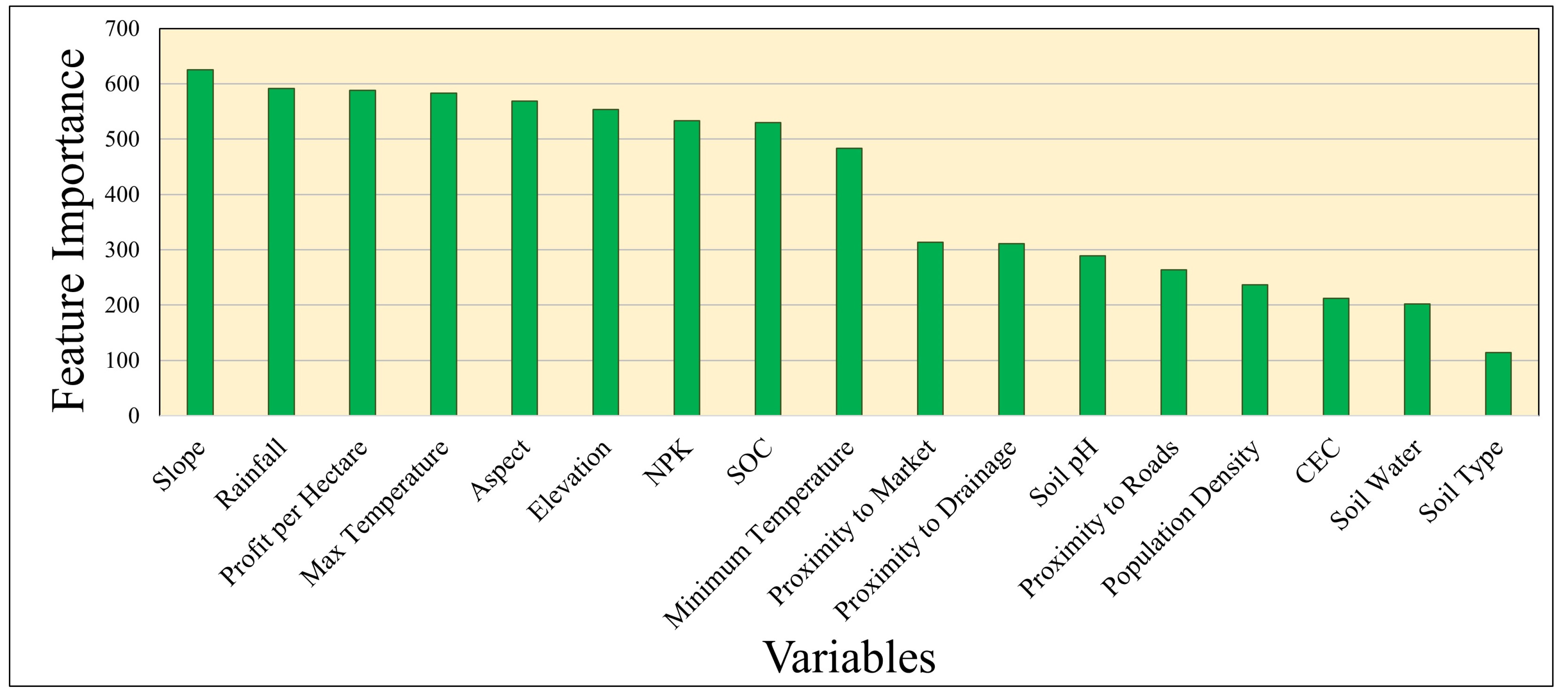
2.2.4. Feature Importance Computation

Sample points representing various crop types were extracted from the crop pattern map, ensuring proportional distribution based on area coverage. The selected parameters influencing crop patterns were spatially mapped and rescaled to a 10 m resolution across the study area. These rescaled layers were then imported into GEE as predictor variables and crop types as target variables. Eventually, under the random forest regressor algorithm, feature importance analysis was performed to quantify the contribution of individual predictors and their relative significance in determining crop types. Feature importance measures discriminate parameters behaviors, providing importance rankings; thereby, the relative role of variables can also be used to determine any output event [46]. Moreover, it also allows feature importance algorithms to follow this mathematical equation under random forest [47]:
X = 1 n T i = 1   n o d e   j T i |   s p l i t   v a r i a b l e   j = x n T p T i ( j ) i T i ( j )
where X is the average importance of the feature, nT represents the number of trees in the forest, T is the tree, p T i ( j ) represents the fraction of samples reaching node j, and i T i ( j ) is the change in impurity in tree T and node j.

2.2.5. Crop Diversity and Combinations

Patch richness density (PRD) was assessed using Fragstat 3.0 software to identify the distinct number of patch types in the landscape level, indicating patch diversity. The Shannon diversity index (SHDI), which quantifies the landscape diversity, was applied here to estimate crop diversity in croplands. This metric considers the distribution and relative abundance of patch types together to estimate diversity. Subsequently, the mean patch size (MPS) was measured to obtain an overview of the average land size under each crop type across the entire landscape within each block. Furthermore, crop combinations were analyzed using Rafiullah’s [48] deviation method using the following formula.
D = i = 1 n ( P i M ) 2
where D is the deviation of the crop combination, Pi is the percentage of the cropped area occupied by ith crop, and M represents the mean percentage area of all crops under the total cropped area. This deviation can range from 0, with a uniform distribution of multiple crops, to 100, with a monoculture area.

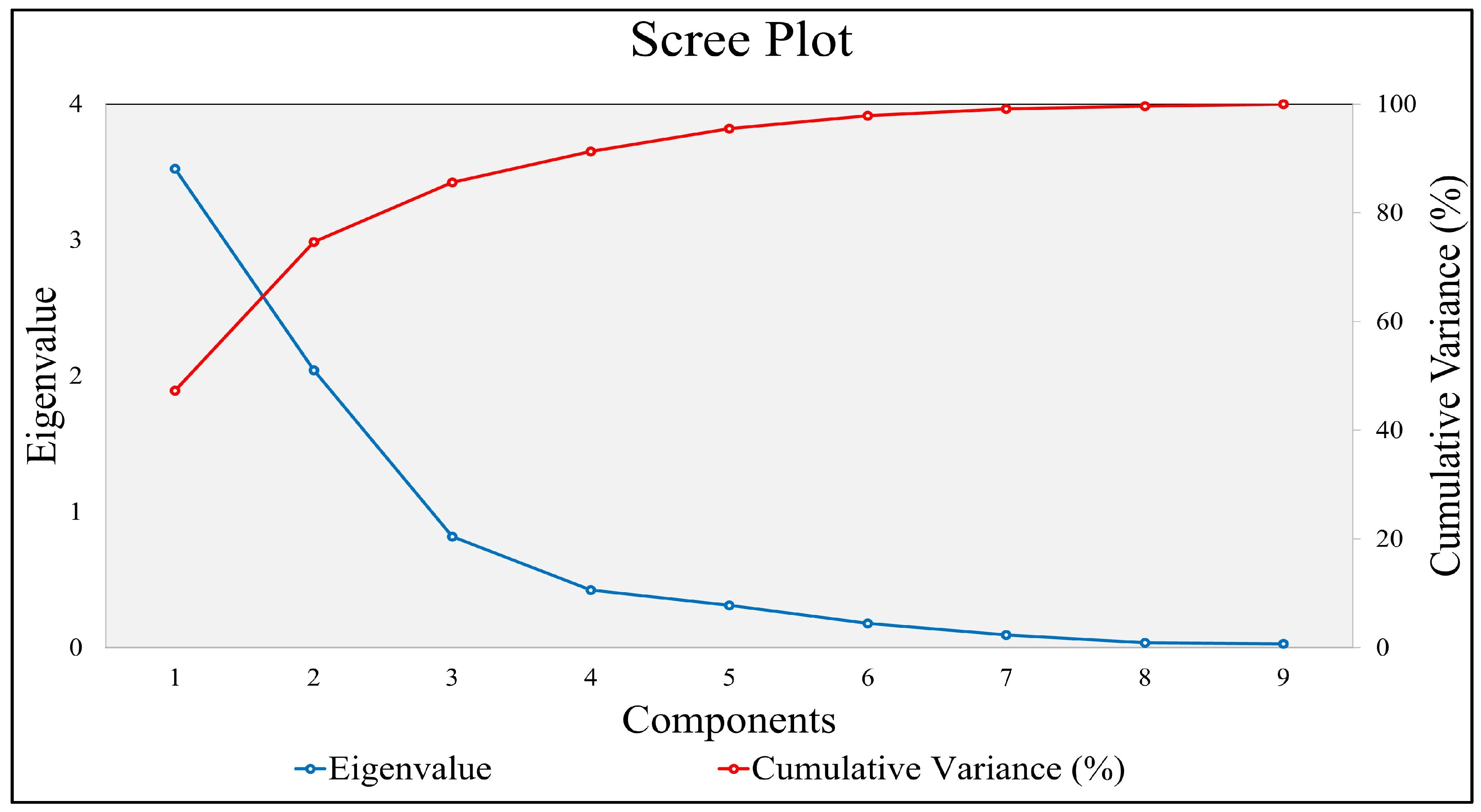
2.2.6. Calculation of Landscape Metrics

Landscape metrics are essential algorithms used to quantify the spatial patterns and fragmentation in a landscape mosaic within a scale [49]. In the present study, the number of patches (NP), patch density (PD), the percentage of the landscape (PLAND), mean patch size (MPS), largest patch index (LPI), edge density (ED), clumpy (CLUMPY), split index (SPLIT), and aggregation index (AI) were chosen to study the fragmentation pattern of different crop fields in each block. The formulas [50] for the metrics are as follows:
P D = N P A × 10 4
L P I = m a x j = 1 m ( a P a t c h ) A × 100
M P S = i = 1 m   a p a t c h f P a t c h   ( 1 10,000 )
E D = e i A × 10 4
P A R A = E x p o s e d   P e r i m e t e r A r e a   o f   S p e c i f i c   C l a s s  
CLUMPY = ( g i e i ) g i   e i p i
SPLIT = A 2 j = 1 m   a i j 2
AI = ( g i g m a x ) × 100
where ‘a’ represents the area of the patch, ‘m’ indicates the number of observations, ‘A’ denotes the total area under the landscape, and ‘ei’ represents the total number of edges under the ith class. PD, ED, and SPLIT are landscape metrics with a lower limit of 0 and an open-ended upper limit. LPI and AI vary from 0 to 100 [30]. CLUMPY varies from −1 to +1. PD specifically denotes how many patches there are within 100 ha. With a higher value, it depicts the dividing tendencies of patches. LPI, on the other hand, assesses the dominance of the largest patch over the entire landscape through the proportion of the largest patch, where a higher value suggests a large contiguous crop cover under a single crop. Edge density measures the total number of lengths of edges within a unit area, where high-density influences the splitting of large lands into smaller patches. CLUMPY tries to find out how the patches under each crop are clumped together or clustered in a spatial unit, considering the shape and edge effect within a patch. Similarly, AI also assesses the aggregation at a spatial level. However, it focuses more on overall connectivity. SPLIT tries to find out how many uniform patches of equal size would result in the same level of fragmentation as the actual landscape. In general, these landscape metrics try to assess the amount of fragmentation with different approaches. Therefore, all these were combined into a single composite metric to obtain an overall picture of fragmentation in this research.

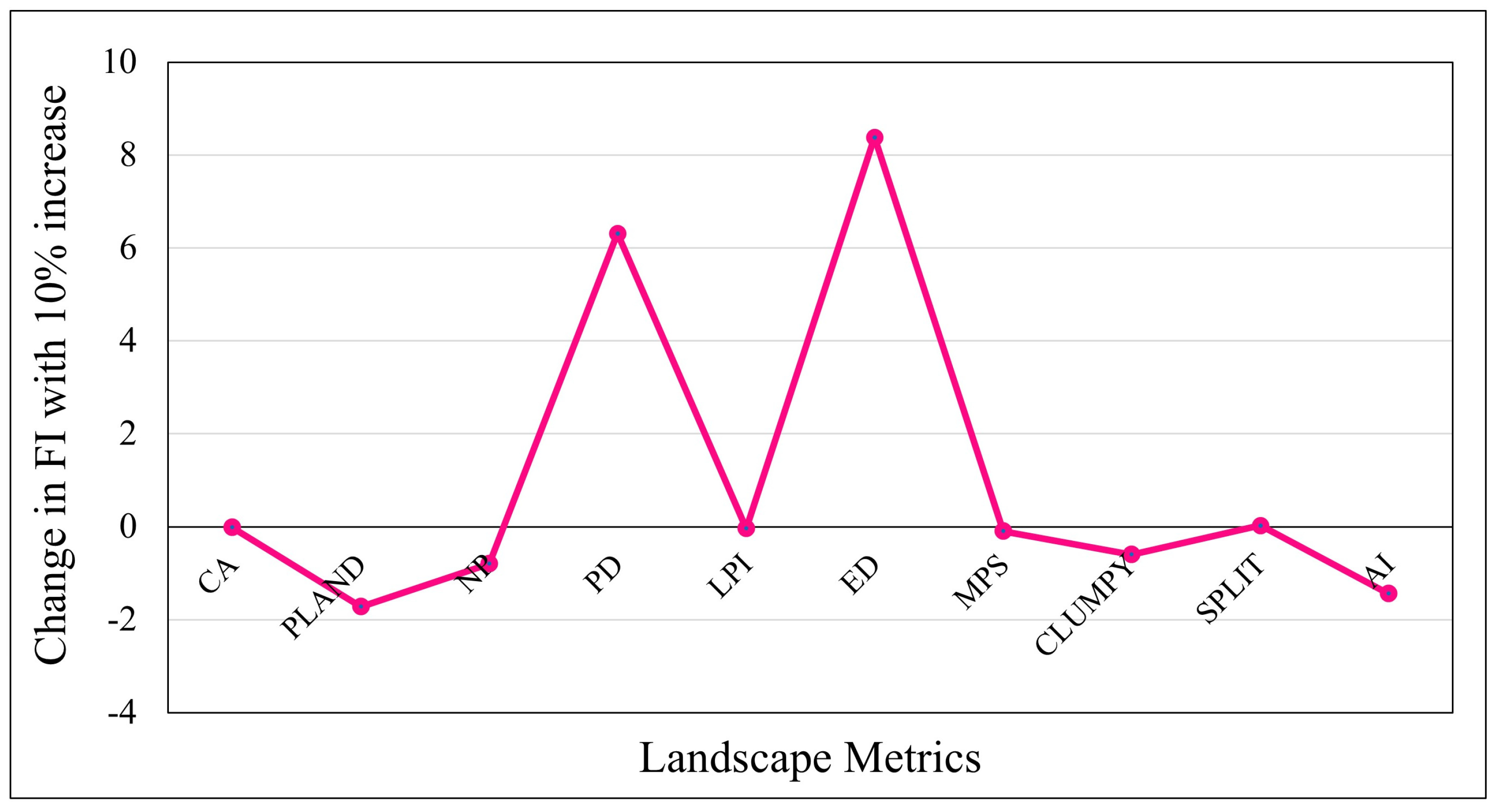
2.2.7. Fragmentation Index

A selected few metrics directly measure the patch dynamics; some evaluate the extent of splitting, while others examine the complexity of the shape and investigate changes in clustering and aggregation. A higher number of patches in some tehsils can be attributed to either fragmentation or simply greater areal coverage. Thus, PD was essential in distinguishing between these causes. Similarly, low PD can indicate crop isolation, which in turn affects ED. The MPS metric was used to understand the average size of crop fields. However, in cases with high variability, misinterpretations could arise. To address this, LPI was included to assess the dominance of a single patch. Aggregation metrics, including CLUMPY and AI, provide a clearer understanding of spatial concentration, while SPLIT values help quantify fragmentation. Together, these metrics offer a comprehensive view of the fragmentation dynamics. Therefore, it is crucial to integrate this diversity. Although a composite index with equal weights could be employed, this approach may not adequately address the varying significance of individual metrics in fragmentation. Moreover, the relationship between fragmentation and these metrics is not uniformly linear; as some metrics exhibit direct proportionality while others are inverse, it becomes essential to consider both types of associations. Banerjee et al. [29] have tried to counter this challenge by assigning weights in combination with the areal change. However, this method is rigorous, localized, and based on subjective weights. For the objective weight estimation, principal component analysis (PCA) was performed on the standardized Z-scores of the metric values in this study.
PCA facilitated the extraction of principal components (PCs) and associated eigenvectors, with the loadings of each metric indicating their contributions to the PCs (Figure 3). Oblimin rotation with Kaiser normalization was applied to refine the loadings, enabling the assignment of appropriate weights to each metric.
As the second PC after PCA emerge to be the most appropriate representation of the theoretical understanding of fragmentation and its relation to these metrics, the component loadings of PC2 were considered for the weight assignment (Table 2).
Based on these weighted contributions, a formula was developed to quantify fragmentation, as follows:
f = i = 1 m ( ω i ×   Z i )
where f represents fragmentation, m is the number of metrics, ωi indicates the weight assigned by the PCA method for the ith metric, and Z is the value of the standardized metric. The robustness of the formula was validated through sensitivity analysis using the one variable at a time (OAT) method. This involved incrementally increasing each variable by 10% to evaluate its impact on fragmentation values. The analysis demonstrated that the changes introduced did not significantly affect the stability of the formula, confirming its reliability for assessing fragmentation (Figure 4). Finally, the results were classified based on equal intervals for all the crops across the study area, as very low (−4.11 to −2.11), low (−2.11 to −0.11), moderate (−0.11 to 1.88), high (1.88 to 2.11), and very high (2.11 to 4.11).

3. Results

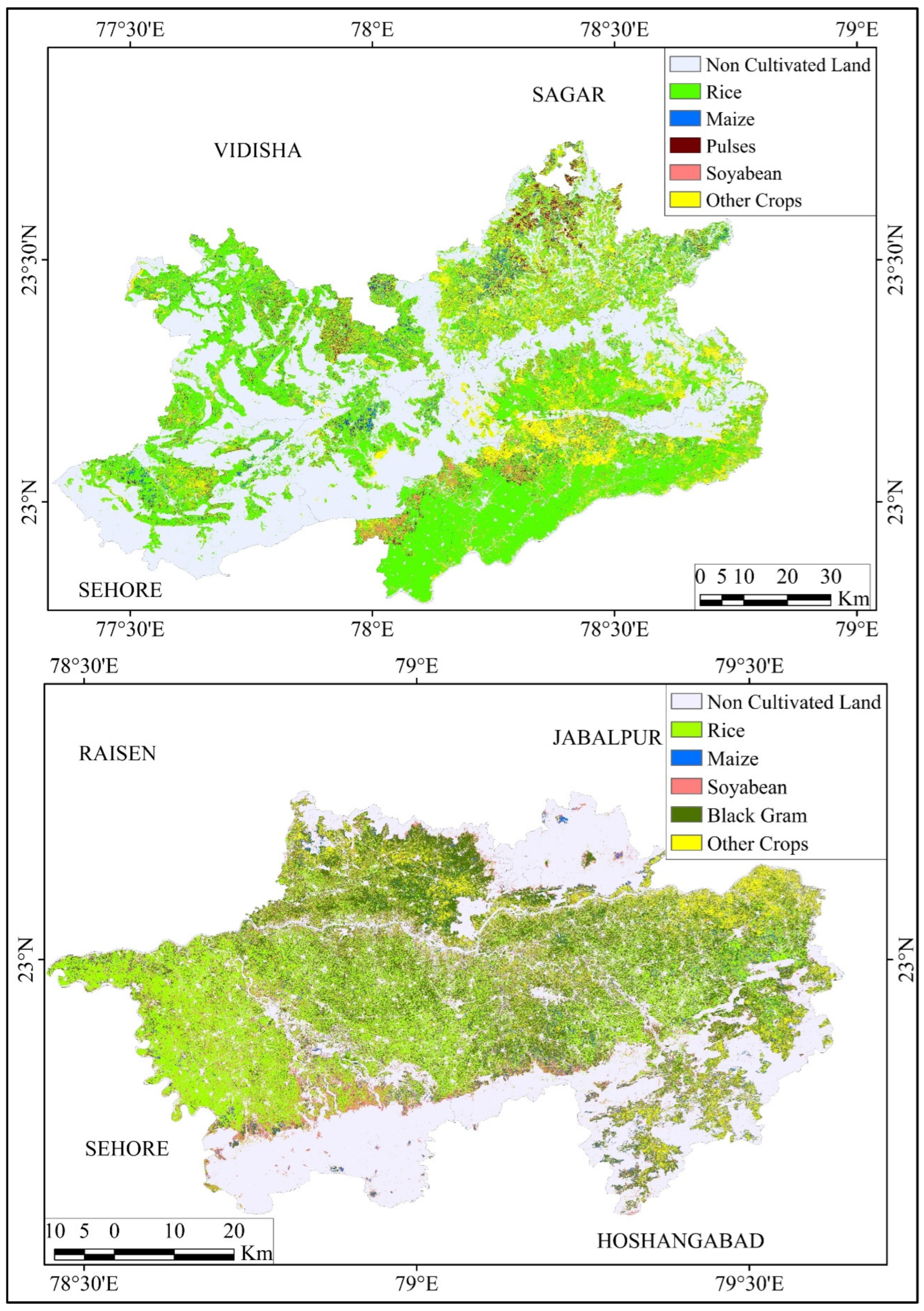
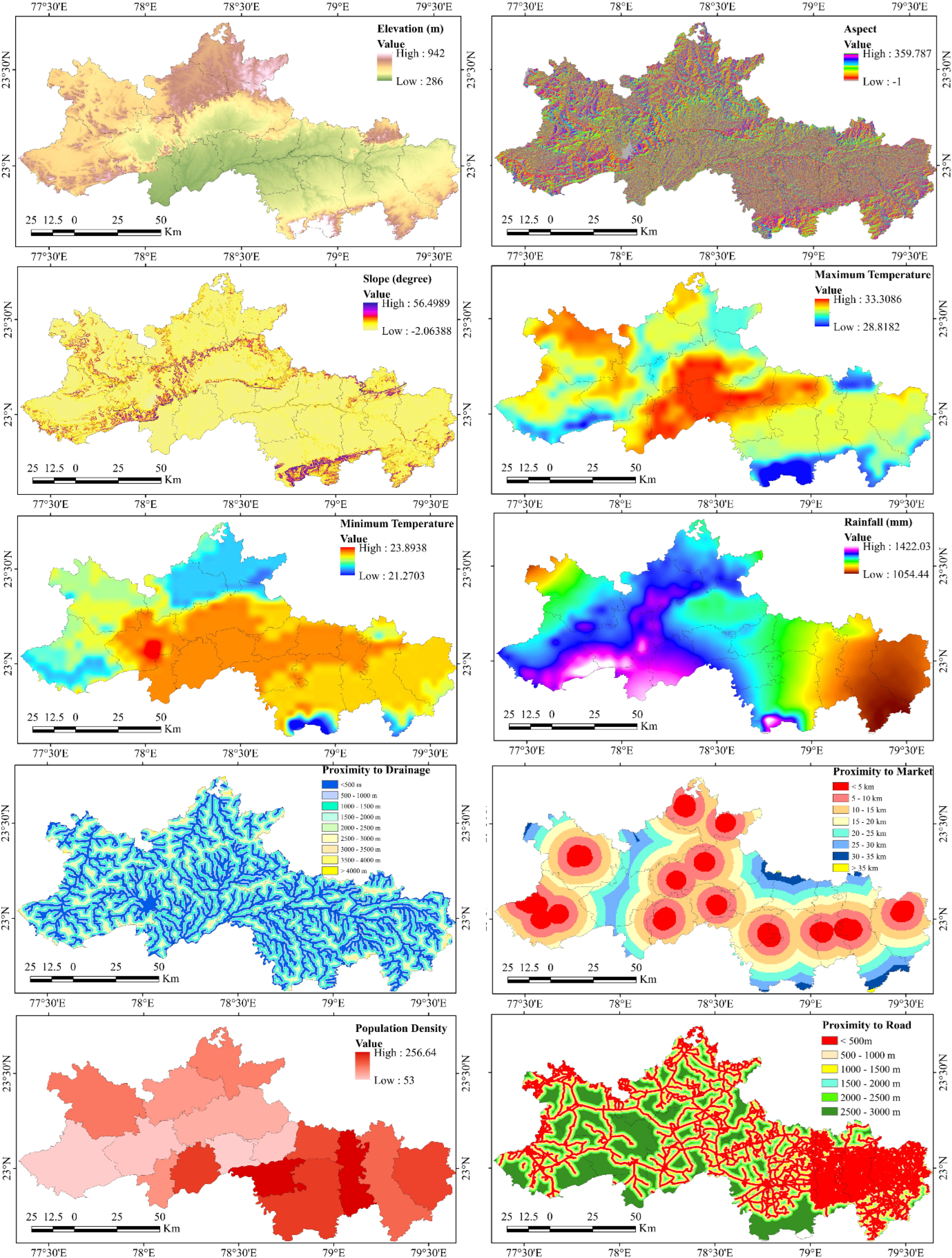
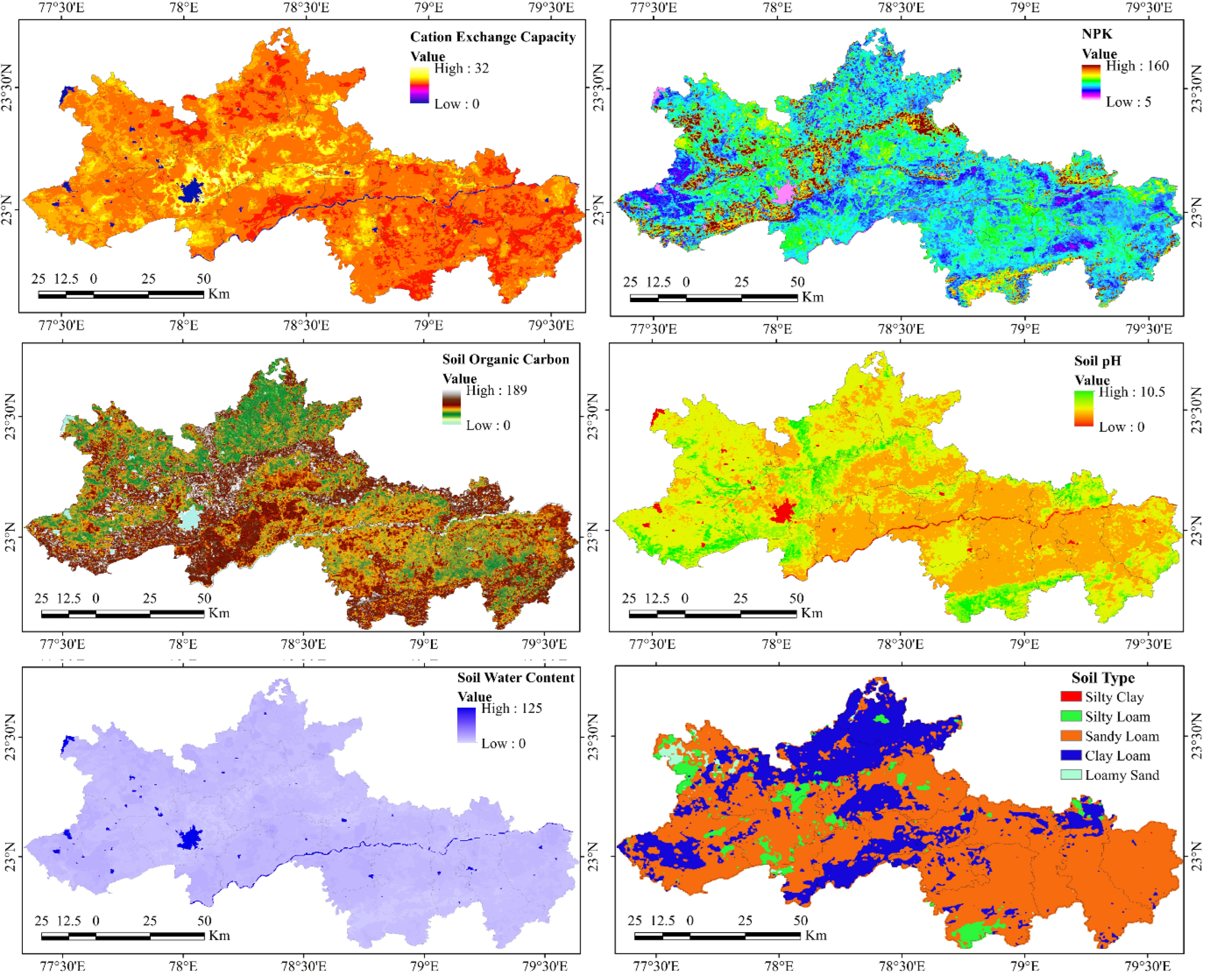
3.1. Crop Pattern and Their Driving Factors

Upon executing the model, a detailed crop-type map was generated. Crops occupying less than 1% of the total cultivated area were categorized as minor crops, while those exceeding this threshold were labelled individually. Rice, soybean, black gram, maize, and pulses were prominent major crops. The term pulses refers to a group of crops, including lentils, chickpeas, green grams, dry peas, and beans. As none of these individually constituted a significant portion of the cultivated area, their collective cultivated area was substantial, warranting grouping them under the category of pulses. An exception was made for black gram, which, despite being a member of the pulse family, occupied a substantial area under cultivation in the Narsinghpur district. Due to its notable prevalence, black gram was classified as a distinct crop type rather than being grouped under pulses in this study.
Random forest-based crop classification with an overall accuracy of 93% and 94%followed by a Kappa coefficient of 0.9 and 0.89 for Raisen and Narsighpur (Table 3), respectively, revealed a distinct and heterogeneous crop pattern throughout the region (Figure 5); it was accurate in Kharif season, as we have taken only this season. Rice emerged as the most important crop in Raisen with 40% (347,413 ha) of the total area and highest FI score (Table 4), mainly concentrated in the alluvial plain of the Narmada Valley. Meanwhile, in Narsinghpur, black gram surpassed rice and other crops to become the most cultivated crop. Pulses are clustered in the northern part of Raisen, specifically in Begamganj Tehsil; whereas, maize and soybeans are cultivated in a dispersed manner. In Narsinghpur, sobangkok maldaybeans also had a significant presence, along with black gram and rice. However, soybean, maize, and black gram often overlapped with simultaneous presence in the same areas due to intercropping. Horticultural crops, such as vegetables and fruits, were also present in a scattered manner throughout both districts.
Overall, rice fields in both districts are predominantly located in areas with gentle slopes, clay-based wet soils and the fertile alluvium of the Narmada Valley. Conversely, pulses are associated with drier areas and highland regions, such as the Vindhyan and Satpura ranges. A remarkable amount of land was fallow land due to low agricultural productivity.
Here, we tried to show the spatial alignment and spatial relationship; thus, it was identified that where gentle slopes and wet soils are present, in the majority of the places, rice was seen growing. Whereas, pulses were found at highland areas with drier conditions. This can be understood, if we see the slope, elevation, precipitation, and crop distribution maps together.
The feature importance of random forest algorithm uncovered that slope, rainfall, and profit per hectare as the most critical factors in determining crop patterns, with relative importance scores of 625.17, 591.27, and 588.35, respectively (Figure 6). Gentle slopes, typically associated with rice, soybean, and black gram cultivation, exhibited high agricultural activity. Meanwhile, moderate slopes were more favorable for maize and pulse production, particularly at altitudes of 495–580 m. Conversely, steep slopes remained largely uncultivated due to rocky or forested terrain (Figure 7). Rainfall plays a decisive role in crop patterns. Areas with rocky surfaces and steep gradients, despite receiving the highest rainfall, remain unsuitable for agriculture due to the high slope. In contrast, the foothills, receiving 1100–1200 mm of rainfall, form highly productive rice belts. The eastern parts of Narsinghpur were significantly drier to support rice; thus, soybean, black gram, and minor crops became popular choices for farmers.
As a bioclimatic variable, the temperature range also significantly influences crop patterns. Maximum temperature (582.83), aspect (568.8), and elevation (553.72) also emerged as critical factors. Southern- and eastern-facing slopes are characterized by more sunlight, favoring agricultural growth. Lower elevations with gentle slopes supported black grams and rice dominance, while increasing elevation and slope increased the diversity and dominance of maize and pulses. Dense forests and barren lands are found at more than 600 m elevation with minimum human intervention (Figure 7).
Edaphic factors, such as NPK (532.85) and SOC (529.58), were highly important due to their supply of crop nutrition. High nutrient uptakes were found in agricultural lands with lower concentrations of NPK; however, pulse fields were an exception. Soil properties, such as soil type (111.4), soil water content (201.07), and cation exchange capacity (211.92), were less significant. The homogeneity in soil type and low variation in soil moisture are probably due to monsoon rainfall (Figure 8).
Anthropogenic factors, such as proximity to markets (313.52), proximity to roads (263.95), proximity to drainage networks (311.044), and population density (236.42), were more important variables for the model in homogenous landscapes (Figure 6).

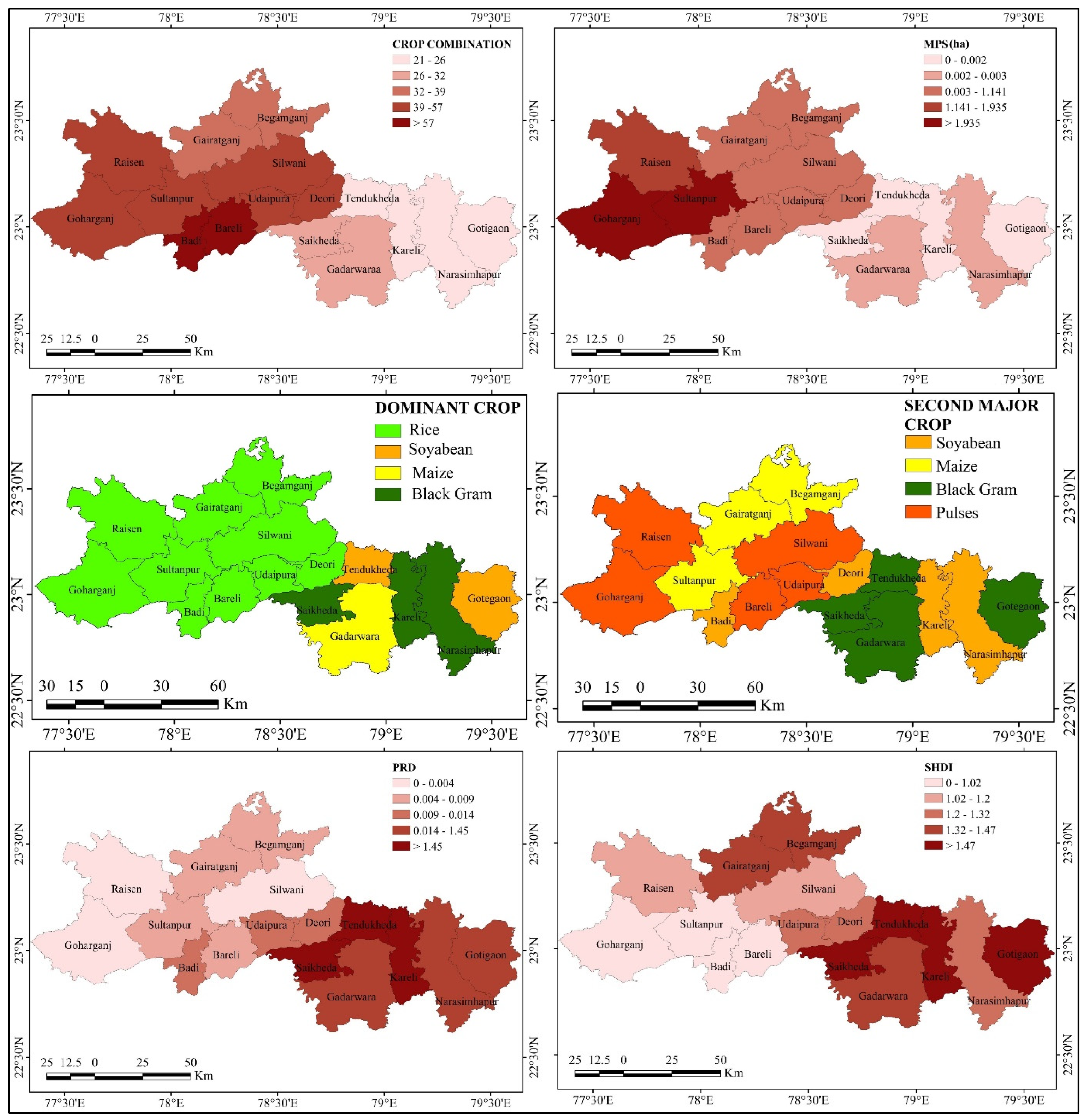
3.2. Crop Combination and Diversity Status

The deviation method of crop combination revealed Bareli in the Raisen district had the lowest combination with a 67.03 deviation, and Gotegaon in Narsighpur had the highest crop combination with a deviation of 21.13. The majority of the tehsils in the Raisen district recorded high deviation, indicating a tendency towards monocropping. In contrast, all the tehsils of the Narsighpur district had a deviation from 21.13 to 32.73, representing a balanced crop combination, probably due to intercropping practices. Balanced crop combinations reduced the average firm size under each crop. Consequently, tehsils like Tendukheda and Saikheda in the Narsighpur district had the smallest average size of land (under 0.002 ha). Within a hectare area, farmers in these regions, on average, planted more than two to three major crops to reduce the risk of crop failure (PRD 2.54 to 2.91). Conversely, the maximum tehsils of the Raisen district exhibited lower PRD, such as 0.005, with a large average firm size ranging from 3 to 3.5 ha. Low population density could be another reason for higher per capita land use.
The crop dominance assessment also uncovered the prevalence of monocropping in Raisen, with a wide gap between the area of coverage (need a table) for the most cultivated crop and the second most cultivated crop. Rice had a coverage ranging from 20% to 73% of the total geographical area per tehsil, while maize (the second most dominant crop) covered only 2% to 10%. Narsinghpur, however, exhibited a more balanced crop distribution, with a smaller gap between the dominant and secondary crops.
The crop diversity was further quantified using SHDI (explained in Section 2.2.5.) (Figure 9). Sultanpur, Badi, and Bareli in Raisen exhibited the lowest diversity, with SHDI values of 0.92, 0.95, and 0.98, respectively, as the combination values indicated. In Badi and Bareli, the fertile alluvial soils supported high rice yields, while in Sultanpur, abundant monsoonal rainfall (1400 mm) favored rice cultivation. However, slightly acidic soils, combined with low accessibility to markets and roads, limited the cultivation of pulses, horticulture, and other crops in Sultanpur. Consequently, rice accounted for 66%, 78%, and 80% of the cultivated land in Sultanpur, Badi, and Bareli, respectively. On the other hand, Gotegaon and Tendukheda in Narsinghpur had the highest diversity values (1.6 and 1.59 SHDI), reflecting a greater prevalence of intercropping and diversified cropping systems.

3.3. Crop-Specific Landscape Metrics and Fragmentation

Landscape metrics and fragmentation indices revealed a concentrated dominance of rice cultivation in the southern and southeastern tehsils of the Raisen district, with Raisen tehsil exhibiting the highest areal coverage (59,311.90 ha, 37.78%) and Bareli exhibiting the greatest proportional dominance (72.19% of its total area). Conversely, tehsils like Tendukheda, Narsimhapur, Kareli, and Gotegaon in the Narsighpur district had minimum coverage (160–1608 ha, 0.6% 3.8%). This kind of variation reflects the high spatial heterogeneity of rice cultivation. Begamganj in northern Raisen had the highest number of rice fields (47,166) with a PD of 45.03 and an ED of 239.71, followed by Silwani and Gairatganj. The dominance of rice was so visible that some individual fields covered 27.4 to 63.05% of the total geographical areas of respected Tehsils, maintaining good core health. This core rice-growing region (rice belt) demonstrated high aggregation, with CLUMPY values exceeding 0.8 and AI values above 90, coupled with minimal fragmentation as indicated by low SPLIT values ranging from 2.5 to11.97 (Figure 10). Consequently, these tehsils registered very low fragmentation (FI values: −2.11 to −4.11). This dominance was absent in the Narsighpur district, despite the presence of the alluvial plain of Narmada (number of fields 2805–5623 alongside 884–1928 PD and 103–241 ED). Saikheda tehsil recorded the highest PD and ED (7776.2 and 1796.64) among other tehsils, making it the most fragmented (FI: 1.234). Tehsils in the Narsighpur district had high SPLIT values (366,000–27,134,730), low MPS (0.006–0.02 ha), negligible clustering, and the presence of cold spots (p < 0.05) of rice contributing to higher overall fragmentation values. Overall, rice fields throughout the study area were not significantly fragmented, ranging from low to moderate fragmentation only.
Similarly, soybeans also exhibited a distinct pattern of concentration that is contrasting to rice, with notable heterogeneity. The highest area coverage was recorded in Gotegaon (8873.32 ha, 21.44%), while Tendukheda had the greatest proportional dominance (26.89%). Tehsils such as Sultanpur, Saikheda, and Begamganj showed minimal soybean coverage (898–1048 ha, 0.8% 4.5%). This smaller gap between the highest and the lowest coverage indicates lower variability and a higher balanced distribution of soybeans compared to rice. Eastern peripheral tehsils recorded the highest soybean productivity and areal coverage, along with the highest PD (18,091.31–25,235.90) and ED (2116–3562). Smaller mean field sizes (0.0006–0.0011 ha) were the reason behind the increase in PD and ED (Figure 10). Consequently, the number of soybean fields in these tehsils (51,959–97,737) nearly doubled the number of tehsils with the maximum rice fields. As a result, tehsils in the eastern periphery of the Narsighpur district exhibited the highest fragmentation value (FI: 5.03–5.82) despite higher areal coverage. The rice belt in the Raisen district had fewer soybean fields (10,344–15,831) and lower PD (10.002–34.92) despite larger field sizes (0.08–0.25 ha). Clustering metrics exhibited the lowest CLUMPY (<0.461) and AI (<46.62) values, along with extremely high SPLIT values (>22,814,628.01), indicating highly fragmented and randomly distributed soybean fields. Overall, soybean fields were found to be smaller and more fragmented than rice fields across all tehsils. Exceptionally, Badi, despite being part of the rice belt, showed a significant soybean cluster (CLUMPY 0.73, AI 74.48, SPLIT 24,100), probably due to the presence of isolated pockets of soybean fields with larger mean patch size rather than the genuine connectivity of soybean fields.
On the other hand, maize fields did not form any specific zone; instead, they were spread in a dispersed manner. Gadarwara tehsil had the highest areal coverage (12,233.53 ha, 19.64%) and number of fields (86,107), while its northwestern neighbor, Saikheda, exhibited the greatest proportional dominance (32.59% of its total area), with the largest LPI (4.89%), the highest PD (17,330.11) and ED (3955.95), and a very low MPS (0.0019 ha), highlighting significant variability in maize field sizes and eventually the highest degree of fragmentation (FI: 4.83) (Supplementary Table S1). As for soybeans in the case of maize also, Gadarwara and Gotegaon exhibited high PD, ED, and field numbers, despite large areal coverage because of very small field sizes (0.0007–0.0014 ha). Thus, these tehsils were among the most fragmented (FI: more than 3). However, in the rice belt, minimum maize cultivation was observed (0.09% to 1.9%), with lower field numbers (1459–6507), PD (3.4–14.13), and ED (2.46–17.94). Metrics such as CLUMPY and AI revealed that maize cultivation is forming clusters within the northern region of eastern tehsils of the study area near the soybean belt, with CLUMPY and AI exceeding 0.7 and 75, with low SPLIT values (7554.45–54,762.56). Meanwhile, the rice belt lacked significant maize concentrations, with CLUMPY and AI values <0.4 and <48, respectively, and extremely high SPLIT values (>24,428,886.51). Due to very low maize cultivation in isolated pockets of the rice belt, their overall fragmentation value decreased despite high SPLIT values (Figure 11).
Pulses are mainly cultivated in the Raisen district. Begamganj exhibited the highest areal coverage (8719 ha, 8.32%), number of fields (89,602), PD (85.54), ED (113.95), and aggregation metrics (CLUMPY: 0.61, AI: 64.9), indicating highly connected and aggregated fields. Raisen and Gairatganj follow with over 74,000 fields and moderate PD (48.95–70.25) and ED (70–73). Meanwhile, Sultanpur showed limited pulse coverage (1684 ha, 1.84%) and lower PD (25.94) and ED (30.42), which represent the isolation of the fields. Pulses, in general, were found to have a larger field size, higher uniformity, and less fragmentation (FI: −2.11 to −0.11).
Black gram, primarily cultivated in the Narsinghpur district, overlaps spatially with soybean and maize, forming a balanced cropping system. Gadarwara leads with the highest coverage (11,773.38 ha, 18.9%), followed by Narasimhapur (7347.45 ha) and Gotegaon (6911.01 ha). Saikheda has the highest proportional coverage (23.52%). Black gram cultivation is widespread across the district, covering 13–23.52% of each tehsil’s area. Unlike the rice belt, where monoculture is common, black gram’s coexistence with soybean and maize reflects a diversified cropping pattern. Gotegaon exhibits the highest PD (21,232.83) and ED (3486.35), with small average field sizes (0.0008 ha), which makes it the most fragmented tehsil of black gram fields (FI: 5.89) (Supplementary Table S1). However, Saikheda, Gadarwara, and Kareli show clustering with high aggregation (CLUMPY > 0.7, AI > 71.5) and low SPLIT values, highlighting the spatial concentration of black gram fields. Black gram cultivation in Narsinghpur is marked by small, fragmented fields, high PD and ED, and a balanced crop combination, underscoring its adaptability and importance in the district’s agricultural system.
In the case of the other minor crops, Udaipura, Begamganj, and Gairatganj lead with 28.23%, 26.05%, and 23.11% of the area under multiple minor crops, including green chilies, bottle gourd, bitter gourd, okra, brinjal, cotton, and millets. These wide-ranging crops, classified as other crops, are characterized by a fragmented but diverse agricultural landscape in the Narsinghpur district and are more homogenous in the Raisen district (FI: −1 to 4.14).
Overall, the widespread practice of intercropping in Narsinghpur, characterized by high crop diversity and balanced crop combinations, contributes to higher fragmentation values. At the individual scale, these fragmented fields may appear less productive due to smaller plot sizes and varying crop types. However, when analyzed at a landscape level, this diversity offers several key advantages. A diverse cropping system minimizes competition for resources, optimizes nutrient cycling, and can result in greater cumulative yields across the landscape. Moreover, intercropping systems reduce the vulnerability of the agricultural landscape to extreme weather events, pests, and diseases by spreading risks across multiple crops. In addition, higher biodiversity in intercropping systems enhances ecological stability, supports soil health, and promotes sustainable agricultural practices.

4. Discussion

4.1. Integrating Remote Sensing, Machine Learning, and Landscape Metrics

This study demonstrates the transformative potential of integrating remote sensing, advanced machine learning algorithms, and landscape metrics to comprehensively analyze agricultural landscapes. The use of high-resolution satellite images, such as a Sentinel 2A-based timeseries of NDVI trends during monsoon, to identify the phenological cycle of crops in this research makes the cropland identification more accurate compared to traditional techniques. The application of the RF algorithm to classify the crop type using ground-based crop-type data provided superior classification precision (over 93% accuracy). The assessment of importance and rank quantified the role of various drivers in determining crop patterns. Furthermore, the integration of landscape metrics added a new dimension to the understanding of spatial patterns and structures of crop fields. Combining these metrics to construct an index for measuring fragmentation and using PCA-weighted methods, this study overcame the subjectivity and theoretical bias seen in previous attempts. The FI presents insights into agricultural planning through targeted intervention, such as identifying areas with high connectivity and resilience (for instance, the rice belt in the study area) and those prone to ecological risks (highly fragmented soybean fields). Metrics like SHDI and PRD effectively identified agricultural land-use diversity and crop diversity supported by crop combination assessment. This integrated approach has significant implications in land use planning, precision agriculture, and climatic resilience. Moreover, the study’s ability to predict pixel-level crop probabilities through RF models provides a valuable tool for site-specific crop management and climate adaptation strategies.

4.2. Interconnection of Crop Pattern, Diversity, and Fragmentation

The present investigation led to an understanding of crop patterns, their drivers, and landscape ecology covering the combination, diversity, and fragmentation of cropland. The combination of climatic and topographic features shaped the suitability zone of different crops. For instance, rice, the most water-reliant crop, thrived in areas with gentle slopes, high rainfall, low soil pH, and the presence of alluvium. At the same time, black gram and soybean grew better in drier conditions due to less competition from rice. High soil pH and low cation exchange capacity also offered advantages to these crops in resource-constrained areas. Spatial overlaps were also common due to the similar climatic tolerance of numerous crops and homogeneity in soil types. For example, the western rice belt also served as a hotspot for pulses, northern Begamganj experienced an overlap of maize and pulses, and the eastern part of the study area frequently exhibited overlapping zones of black gram, soybean, and maize. Anthropogenic drivers outweighed the environmental drivers in choosing specific crops in the areas of common suitability zones of multiple crops. Large-scale monoculture in rice belts was characterized by high vulnerability toward climate-induced hazards despite their low fragmentation and high productivity [51]. Similar to other regions of India, the overuse of chemical pesticides triggered soil degradation and toxic agricultural runoff in the monsoon and compromised the sustainability of land [52,53,54]. Eventually, it hampered the biodiversity of the concerned agroecosystem and the surrounding aquatic and terrestrial ecosystems. In contrast, regions with rugged terrains and red soil were dominated by fragmented land with a preference for intercropping and mixed farming. In Narsinghpur, black gram, soybean, and maize were often grown together, reflecting a balanced crop combination. This enhanced resilience against crop failure, achieved higher cumulative yields, and made more profit compared to monoculture, like many tropical regions [55]. However, these fragmented lands wasted a significant amount of area in boundary delineation (locally known as “aal”). Fragmentation also made large-scale policies, like crop insurance and infrastructure development, more difficult [56]. Due to very low per capita land, owners of these fragmented lands were bound to sell their crops at minimum support prices at local markets. Despite this limitation, crop diversity promoted ecological stability, climatic resilience, and maximum resource utilization, reducing the risk of catastrophes [57,58]. This is how the interaction of fragmentation, diversity, and crop combination shaped the decision making of farmers, land-use patterns, and the livelihood quality of local agriculture-dependent people. The heterogeneity in the landscape, however, underscored the need for policies focusing on sustainability without compromising productivity. Moreover, site-specific targeted intervention is highly required.

4.3. Sustainable Land Use and Resilience to Climate Change

Diversifying crop selection at different levels of climatic tolerance in the Narsinghpur district offers a reduced dependency on a single crop, mitigates the risk of extreme weather conditions, and stabilizes yields, ensuring food security. This kind of intercropping system, specifically with multiple crops from the pulse family, enhances soil health by improving microbe counts and regulating nutrient cycling [59]. This helps to maintain fertility and reduces the need for fertilizers and eventually improves the management of the water cycle [60]. In addition, this system of agriculture is an excellent platform for increasing biodiversity. However, the challenge of fragmentation can be addressed without compromising diversity by creating buffers and integrating agroecological practices.
Incorporating policies such as subsidizing and incentivizing through training programs for local farmers and providing access to resilient crop varieties can build capacity against climate change and toward sustainability in regions of monoculture. As in different regions, such as from existing research in many countries, such as Tanzania and Southeast Asia, it is evident that crop insurance, subsidizing, and providing a variety of crops empower farmers [61,62,63]. The elimination of reliance on single crops led farmers to be least affected by market fluctuations and stabilize their incomes, thus encouraging a balanced crop combination or plantation within rice fields that could improve the overall quality of the landscape [64].

5. Conclusions

This study successfully attempted and investigated crop patterns, diversity, combinations, and fragmentation in agricultural landscapes, integrating the remote sensing data, machine learning techniques, and landscape metrics. The random forest algorithm and its feature importance technique achieved high accuracy (exceeding 90%) in demonstrating the crop pattern and the important factors determining it. This study also made a novel attempt to map crop combinations and diversity using the spatial dimensions of the landscape metrics from classified pixel-level data. The main contribution of the study remains in its development of the comprehensive and scalable fragmentation index, where it counters the subjectivity-based weight assignment techniques used earlier and combines numerous aspects of fragmentation in a single index. This index can be applied in any part of the world, followed by the methodology used for similar kinds of studies. The use of the GEE platform will allow us to implement it at a large spatial scale, also due to its cloud-based computational efficiency. The case study illustrated the distinct pattern of two different districts, with one more dominated by monoculture and another one having a balanced crop combination. The findings inform land use planning by identifying priority zones for land consolidation and precision agriculture. Modifying the agricultural policy based on local focus will reduce spatial disparity in the future. Future research should focus on the application of this framework to different places on the globe to check its scalability and capability.

Supplementary Materials

The following supporting information can be downloaded at: https://www.mdpi.com/article/10.3390/land14061203/s1, Supplementary Table S1: FI score for each crop in each tehsil.

Author Contributions

Conceptualization, S.B. and T.N.; methodology, S.B.; software, S.B.; validation, T.N.; formal analysis, S.B.; investigation, S.B., T.N. and M.Z.; data curation, S.B.; writing—original draft preparation, S.B. and T.N.; writing—review and editing, S.B., V.P.S., W.M., W.S.A., D.A.-H. and M.Z.; visualization, S.B.; supervision, V.P.S.; project administration, M.Z. All authors have read and agreed to the published version of the manuscript.

Funding

This research was funded by Princess Nourah bint Abdulrahman University Researchers Supporting Project number (PNURSP2025R680), Princess Nourah bint Abdulrahman University, Riyadh, Saudi Arabia.

Data Availability Statement

Data will be available upon reasonable request.

Acknowledgments

The authors extend their appreciation to Princess Nourah bint Abdulrahman University Researchers Supporting Project number (PNURSP2025R680), Princess Nourah bint Abdulrahman University, Riyadh, Saudi Arabia. The authors are thankful to the farmers of the Raisen and Narsinghpur districts for allowing them to visit their firms during field-based crop-type data collection. In addition, they are grateful to Indrajit Roychowdhury, University of North Bengal, for his valuable suggestions during the study’s conduction.

Conflicts of Interest

Author TN was employed by the company Agricultural Insurance Company of India during initial days of conduction of the research. The remaining authors declare that the research was conducted in the absence of any commercial or financial relationships that could be constructed as a potential conflict of interest.

References

  1. Lal, R. Soil degradation as a reason for inadequate human nutrition. Food Secur. 2009, 1, 45–57. [Google Scholar] [CrossRef]
  2. Sklenicka, P. Classification of farmland ownership fragmentation as a cause of land degradation: A review on typology, consequences, and remedies. Land Use Policy 2016, 57, 694–701. [Google Scholar] [CrossRef]
  3. D’Odorico, P.; Rosa, L.; Bhattachan, A.; Okin, G.S. Desertification and Land Degradation. In Dryland Ecohydrology; D’Odorico, P., Porporato, A., Wilkinson Runyan, C., Eds.; Springer International Publishing: Cham, Switzerland, 2019; pp. 573–602. Available online: http://link.springer.com/10.1007/978-3-030-23269-6_21 (accessed on 8 April 2025).
  4. Baude, M.; Meyer, B.C.; Schindewolf, M. Land use change in an agricultural landscape causing degradation of soil based ecosystem services. Sci. Total. Environ. 2019, 659, 1526–1536. [Google Scholar] [CrossRef] [PubMed]
  5. Winkler, K.; Fuchs, R.; Rounsevell, M.; Herold, M. Global land use changes are four times greater than previously estimated. Nat. Commun. 2021, 12, 2501. [Google Scholar] [CrossRef]
  6. Mishra, P.K.; Rai, A.; Abdelrahman, K.; Rai, S.C.; Tiwari, A. Land degradation, overland flow, soil erosion, and nutrient loss in the Eastern Himalayas, India. Land 2022, 11, 179. [Google Scholar] [CrossRef]
  7. Altieri, M.A.; Nicholls, C.I.; Henao, A.; Lana, M.A. Agroecology and the design of climate change-resilient farming systems. Agron. Sustain. Dev. 2015, 35, 869–890. [Google Scholar] [CrossRef]
  8. Kim, S.M.; Mendelsohn, R. Climate change to increase crop failure in US. Environ. Res. Lett. 2023, 18, 14014. [Google Scholar] [CrossRef]
  9. Das, K. Traditional Agronomic Practices: Understanding and Mitigating the Risks of Climate Change. In Recent Advancements in Sustainable Agricultural Practices; Yasheshwar, Mishra, A.K., Kumar, M., Eds.; Springer Nature: Singapore, 2024; pp. 43–79. Available online: https://link.springer.com/10.1007/978-981-97-2155-9_3 (accessed on 8 April 2025).
  10. Nath, P.K.; Behera, B. A critical review of impact of and adaptation to climate change in developed and developing economies. Environ. Dev. Sustain. 2011, 13, 141–162. [Google Scholar] [CrossRef]
  11. Roy, S.; Hazra, S.; Chanda, A. Changing characteristics of meteorological drought and its impact on monsoon-rice production in sub-humid red and laterite zone of West Bengal, India. Theor. Appl. Climatol. 2023, 151, 1419–1433. [Google Scholar] [CrossRef]
  12. Ogwu, M.C.; Izah, S.C.; Ntuli, N.R.; Odubo, T.C. Food security complexities in the global south. In Food Safety and Quality in the Global South; Springer: Berlin/Heidelberg, Germany, 2024; pp. 3–33. Available online: https://link.springer.com/chapter/10.1007/978-981-97-2428-4_1 (accessed on 9 April 2025).
  13. Pattanayak, A.; Srinivasan, M.; Kumar, K.K. Crop Diversity and Resilience to Droughts: Evidence from Indian Agriculture. Rev. Dev. Change 2023, 28, 166–188. [Google Scholar] [CrossRef]
  14. Ju, F.; Yang, R.; Yang, C. Analysis of Spatiotemporal Dynamics and Driving Factors of China’s Nationally Important Agricultural Heritage Systems. Agriculture 2025, 15, 221. [Google Scholar] [CrossRef]
  15. Kumar, R.; Bhanu, M.; Mendes-Moreira, J.; Chandra, J. Spatio-Temporal Predictive Modeling Techniques for Different Domains: A Survey. ACM Comput. Surv. 2025, 57, 1–42. [Google Scholar] [CrossRef]
  16. Wang, X.; Zhang, J.; Wang, X.; Wu, Z.; Prodhan, F.A. Incorporating Multi-Temporal Remote Sensing and a Pixel-Based Deep Learning Classification Algorithm to Map Multiple-Crop Cultivated Areas. Appl. Sci. 2024, 14, 3545. [Google Scholar] [CrossRef]
  17. Chowdhury, M.S. Comparison of accuracy and reliability of random forest, support vector machine, artificial neural network and maximum likelihood method in land use/cover classification of urban setting. Environ. Chall. 2024, 14, 100800. [Google Scholar] [CrossRef]
  18. Yimer, S.M.; Bouanani, A.; Kumar, N.; Tischbein, B.; Borgemeister, C. Comparison of different machine-learning algorithms for land use land cover mapping in a heterogenous landscape over the Eastern Nile river basin, Ethiopia. Adv. Space Res. 2024, 74, 2180–2199. [Google Scholar] [CrossRef]
  19. Aryal, J.; Sitaula, C.; Frery, A.C. Land use and land cover (LULC) performance modeling using machine learning algorithms: A case study of the city of Melbourne, Australia. Sci. Rep. 2023, 13, 13510. [Google Scholar] [CrossRef]
  20. Kasahun, M.; Legesse, A. Machine learning for urban land use/cover mapping: Comparison of artificial neural network, random forest and support vector machine, a case study of Dilla town. Heliyon 2024, 10, e39146. Available online: https://www.cell.com/heliyon/fulltext/S2405-8440(24)15177-8 (accessed on 9 April 2025). [CrossRef] [PubMed]
  21. Feng, S.; Zhao, J.; Liu, T.; Zhang, H.; Zhang, Z.; Guo, X. Crop type identification and mapping using machine learning algorithms and sentinel-2 time series data. IEEE J. Sel. Top. Appl. Earth Obs. Remote Sens. 2019, 12, 3295–3306. [Google Scholar] [CrossRef]
  22. Rasti, P.; Ahmad, A.; Samiei, S.; Belin, E.; Rousseau, D. Supervised image classification by scattering transform with application to weed detection in culture crops of high density. Remote Sens. 2019, 11, 249. [Google Scholar] [CrossRef]
  23. Erdanaev, E.; Kappas, M.; Wyss, D. The Identification of Irrigated Crop Types Using Support Vector Machine, Random Forest and Maximum Likelihood Classification Methods with Sentinel-2 Data in 2018: Tashkent Province, Uzbekistan. Int. J. Geoinformatics 2022, 18, 37–53. Available online: https://www.researchgate.net/profile/Elbek-Erdanaev-2/publication/360672412_The_Identification_of_Irrigated_Crop_Types_Using_Support_Vector_Machine_Random_Forest_and_Maximum_Likelihood_Classification_Methods_with_Sentinel-2_Data_in_2018_Tashkent_Province_Uzbekistan/links/6284dd9519994305918ec116/The-Identification-of-Irrigated-Crop-Types-Using-Support-Vector-Machine-Random-Forest-and-Maximum-Likelihood-Classification-Methods-with-Sentinel-2-Data-in-2018-Tashkent-Province-Uzbekistan.pdf (accessed on 8 April 2025).
  24. Ahmad, A.; Saraswat, D.; El Gamal, A. A survey on using deep learning techniques for plant disease diagnosis and recommendations for development of appropriate tools. Smart Agric. Technol. 2023, 3, 100083. [Google Scholar] [CrossRef]
  25. Wu, B.; Zhang, M.; Zeng, H.; Tian, F.; Potgieter, A.B.; Qin, X.; Loupian, E. Challenges and opportunities in remote sensing-based crop monitoring: A review. Natl. Sci. Rev. 2023, 10, nwac290. [Google Scholar] [CrossRef] [PubMed]
  26. Siotra, V.; Kumari, S. Assessing spatiotemporal patterns of crop combination and crop concentration in Jammu Division of Jammu and Kashmir. J. Soc. Econ. Dev. 2024, 1–28. [Google Scholar] [CrossRef]
  27. Kumar, M.; Denis, D.M.; Singh, S.K.; Szabó, S.; Suryavanshi, S. Landscape metrics for assessment of land cover change and fragmentation of a heterogeneous watershed. Remote Sens. Appl. Soc. Environ. 2018, 10, 224–233. [Google Scholar] [CrossRef]
  28. Ntshanga, N.K.; Procheş, S.; Slingsby, J.A. Assessing the threat of landscape transformation and habitat fragmentation in a global biodiversity hotspot. Austral Ecol. 2021, 46, 1052–1069. [Google Scholar] [CrossRef]
  29. Banerjee, S.; Sati, V.P.; Almazroui, M.; Chakraborty, S. Spatio-Temporal Assessment of Areal Fragmentation and Volume of Snow Cover in the Central Himalaya. Earth Syst. Environ. 2024, 8, 1639–1656. [Google Scholar] [CrossRef]
  30. Sati, V.P.; Banerjee, S.; Roy, C. Land Use and Land Cover Dynamics and Factors Affecting It in the Central Himalaya. Available online: https://www.researchgate.net/profile/Vishwambhar-Sati/publication/383123033_Land_Use_and_Land_Cover_Dynamics_and_Factors_Affecting_It_in_The_Central_Himalaya/links/66bdc0078d00735592528a0a/Land-Use-and-Land-Cover-Dynamics-and-Factors-Affecting-It-in-The-Central-Himalaya.pdf (accessed on 9 April 2025).
  31. Rogan, J.; Wright, T.M.; Cardille, J.; Pearsall, H.; Ogneva-Himmelberger, Y.; Riemann, R.; Riitters, K.; Partington, K. Forest fragmentation in Massachusetts, USA: A town-level assessment using Morphological spatial pattern analysis and affinity propagation. GIScience Remote Sens. 2016, 5, 506–519. [Google Scholar] [CrossRef]
  32. Kowe, P.; Mutanga, O.; Dube, T. Advancements in the remote sensing of landscape pattern of urban green spaces and vegetation fragmentation. Int. J. Remote Sens. 2021, 42, 3797–3832. [Google Scholar] [CrossRef]
  33. De Matos, T.P.V.; De Matos, V.P.V.; De Mello, K.; Valente, R.A. Protected areas and forest fragmentation: Sustainability index for prioritizing fragments for landscape restoration. Geol. Ecol. Landsc. 2021, 5, 19–31. [Google Scholar] [CrossRef]
  34. Jumani, S.; Deitch, M.J.; Valle, D.; Machado, S.; Lecours, V.; Kaplan, D.; Krishnaswamy, J.; Howard, J. A new index to quantify longitudinal river fragmentation: Conservation and management implications. Ecol. Indic. 2022, 136, 108680. [Google Scholar] [CrossRef]
  35. Sahu, S. Fluvio-dynamics and Groundwater System in the Narmada River Basin, India. In Riverine Systems: Understanding the Hydrological, Hydrosocial and Hydro-Heritage Dynamics; Springer: Berlin/Heidelberg, Germany, 2022; pp. 171–185. Available online: https://link.springer.com/chapter/10.1007/978-3-030-87067-6_10 (accessed on 9 April 2025).
  36. Duhan, D.; Pandey, A.; Gahalaut, K.P.S.; Pandey, R.P. Spatial and temporal variability in maximum, minimum and mean air temperatures at Madhya Pradesh in central India. Comptes Rendus Geosci. 2013, 345, 3–21. [Google Scholar] [CrossRef]
  37. Singh, G.; Singh, B.; Tomar, U.K.; Sharma, S. A Manual for Dryland Afforestation and Management. Scientific Publishers-AFARI: Jodhpur, India, 2017. Available online: https://books.google.com/books?hl=en&lr=&id=8BWNDwAAQBAJ&oi=fnd&pg=PP1&dq=Singh,+G.,+Singh,+B.,+Tomar,+U.+K.,+%26+Sharma,+S.+(2017).+A+manual+for+dryland+afforestation+and+management.+Scientific+Publishers-AFARI.&ots=QNAvXr-BZe&sig=Mq08fVVAF-lbZpSZviWkFzvAQug (accessed on 9 April 2025).
  38. Inglada, J.; Arias, M.; Tardy, B.; Hagolle, O.; Valero, S.; Morin, D.; Dedieu, G.; Sepulcre, G.; Bontemps, S.; Defourny, P.; et al. Assessment of an operational system for crop type map production using high temporal and spatial resolution satellite optical imagery. Remote Sens. 2015, 7, 12356–12379. [Google Scholar] [CrossRef]
  39. Rajput, D.; Wang, W.J.; Chen, C.C. Evaluation of a decided sample size in machine learning applications. BMC Bioinform. 2023, 24, 48. [Google Scholar] [CrossRef]
  40. Amankulova, K.; Farmonov, N.; Abdelsamei, E.; Szatmári, J.; Khan, W.; Zhran, M.; Rustamov, J.; Akhmedov, S.; Sarimsakov, M.; Mucsi, L. A Novel Fusion Method for Soybean Yield Prediction Using Sentinel-2 and PlanetScope Imagery. IEEE J. Sel. Top. Appl. Earth Obs. Remote Sens. 2024, 17, 13694–13707. [Google Scholar] [CrossRef]
  41. Hasan, M.M.; Pramanik, M.; Alam, I.; Kumar, A.; Avtar, R.; Zhran, M. Assessing the efficacy of artificial intelligence based city-scale blue green infrastructure mapping using Google Earth Engine in the Bangkok metropolitan region. J. Urban Manag. 2024, 14, 434–450. [Google Scholar] [CrossRef]
  42. Pappaka, R.K.; Nakkala, A.B.; Badapalli, P.K.; Gugulothu, S.; Anguluri, R.; Hasher, F.F.B.; Zhran, M. Machine Learning-Driven Groundwater Potential Zoning Using Geospatial Analytics and Random Forest in the Pandameru River Basin, South India. Sustainability 2025, 17, 3851. [Google Scholar] [CrossRef]
  43. Mondal, S.; Parveen, M.T.; Alam, A.; Rukhsana Islam, N.; Calka, B.; Bashir, B.; Zhran, M. Future Site Suitability for Urban Waste Management in English Bazar and Old Malda Municipalities, West Bengal: A Geospatial and Machine Learning Approach. ISPRS Int. J. Geo-Inf. 2024, 13, 388. [Google Scholar] [CrossRef]
  44. Diksha; Mishra, V.N.; Kumar, D.; Kumari, M.; Bashir, B.; Pramanik, M.; Zhran, M. Dynamic Quantification and Characterization of Spatial Heterogeneity in Mid-Sized Urban Landscape of India. Land 2024, 13, 1989. [Google Scholar] [CrossRef]
  45. Badola, S.; Pandey, M.; Mishra, V.N.; Parkash, S.; Zhran, M. Landslide Susceptibility Mapping in Complex Topo-Climatic Himalayan Terrain, India Using Machine Learning Models: A Comparative Study of XGBoost, RF and ANN. Geol. J. 2025. [Google Scholar] [CrossRef]
  46. Fang, G.; Wang, C.; Dong, T.; Wang, Z.; Cai, C.; Chen, J.; Liu, M.; Zhang, H. A Landscape-Clustering Zoning Strategy to Map Multi-Crops in Fragmented Cropland Regions Using Sentinel-2 and Sentinel-1 Imagery with Feature Selection. Agriculture 2025, 15, 186. [Google Scholar] [CrossRef]
  47. Breiman, L.; Friedman, J.; Olshen, R.A.; Stone, C.J. Classification and Regression Trees. Routledge. 2017. Available online: https://www.taylorfrancis.com/books/mono/10.1201/9781315139470/classification-regression-trees-leo-breiman-jerome-friedman-olshen-charles-stone (accessed on 8 April 2025).
  48. Rafiullah, S.M. A new approach to functional classification of towns. Geographer 1965, 12, 40–53. [Google Scholar]
  49. Turner, M.G. Spatial and temporal analysis of landscape patterns. Landsc Ecol. 1990, 4, 21–30. [Google Scholar] [CrossRef]
  50. McGarigal, K. FRAGSTATS Help; University of Massachusetts: Amherst, MA, USA, 2015. [Google Scholar]
  51. Mihrete, T.B.; Mihretu, F.B. Crop Diversification for Ensuring Sustainable Agriculture, Risk Management and Food Security. Glob. Chall. 2025, 9, 2400267. [Google Scholar] [CrossRef]
  52. Shukla, A.K.; Singh, A.; Banerjee, T.; Chaudhary, S.K. Impact of Agricultural Chemical Inputs on Human Health and Environment in India. Agric. Chem. Inputs 2021. [Google Scholar]
  53. Shukla, A.K.; Behera, S.K.; Chaudhari, S.K.; Singh, G. Fertilizer use in Indian agriculture and its impact on human health and environment. Indian J. Fertil. 2022, 18, 218–237. [Google Scholar]
  54. Chakraborty, S.K. River Pollution and Perturbation: Perspectives and Processes. In Riverine Ecology Volume 2; Springer International Publishing: Cham, Switzerland, 2021; pp. 443–530. Available online: https://link.springer.com/10.1007/978-3-030-53941-2_5 (accessed on 8 April 2025).
  55. Cho, S.; Yoon, H. Evaluating the economic and environmental benefits of rice-soybean diversification in South Korea. Agric. Syst. 2025, 224, 104258. [Google Scholar] [CrossRef]
  56. Deininger, K.; Savastano, S.; Carletto, C. Land fragmentation, cropland abandonment, and land market operation in Albania. World Dev. 2012, 40, 2108–2122. [Google Scholar] [CrossRef]
  57. Guja, M.M.; Bedeke, S.B. Smallholders’ climate change adaptation strategies: Exploring effectiveness and opportunities to be capitalized. Environ. Dev. Sustain. 2024. Available online: https://link.springer.com/10.1007/s10668-024-04750-y (accessed on 8 April 2025).
  58. Ononogbo, C.; Ohwofadjeke, P.O.; Chukwu, M.M.; Nwawuike, N.; Obinduka, F.; Nwosu, O.U.; Ugenyi, A.U.; Nzeh, I.C.; Nwosu, E.C.; Nwakuba, N.R.; et al. Agricultural and environmental sustainability in nigeria: A review of challenges and possible eco-friendly remedies. Environ. Dev. Sustain. 2024, 1–47. [Google Scholar] [CrossRef]
  59. Singh, R.; Hasanain, M.; Babu, S.; Nath, C.P.; Ansari, M.A.; Kumar, A.; Sofi, M.U.D.; Kumar, S.; Kumar, S. Organic pulse production: Exploring opportunities and overcoming challenges. J. Food Legum. 2024, 37, 144–162. [Google Scholar] [CrossRef]
  60. Layek, J.; Das, A.; Mitran, T.; Nath, C.; Meena, R.S.; Yadav, G.S.; Shivakumar, B.G.; Kumar, S.; Lal, R. Cereal+Legume Intercropping: An Option for Improving Productivity and Sustaining Soil Health. In Legumes for Soil Health and Sustainable Management; Meena, R.S., Das, A., Yadav, G.S., Lal, R., Eds.; Springer Singapore: Singapore, 2018; pp. 347–386. Available online: http://link.springer.com/10.1007/978-981-13-0253-4_11 (accessed on 9 April 2025).
  61. Chemeris, A.; Liu, Y.; Ker, A.P. Insurance subsidies, climate change, and innovation: Implications for crop yield resiliency. Food Policy 2022, 108, 102232. [Google Scholar] [CrossRef]
  62. Gwambene, B.; Saria, J. Smallholder Farmers’ Resilience in Adapting to Climate Changes in the Southern Highlands of Tanzania. J. Geogr. Assoc. Tanzan. 2024, 44, 1–25. [Google Scholar] [CrossRef]
  63. Jat, M.L.; Rao, C.S.; Padmaja-Karanam, V.; Singh, R. Innovations, strategies, and policies for Building Resilience of India’s Dryland Farming to Climate Change. In Climate Change and Sustainable Agro-Ecology in Global Drylands; CABI GB: Wallingford, UK, 2024; pp. 230–252. Available online: https://www.cabidigitallibrary.org/doi/abs/10.1079/9781800624870.0011 (accessed on 9 April 2025).
  64. Frison, E. From industrial agriculture to diversified agroecological systems. Indian J. Plant Genet. Resour. 2016, 29, 237–240. [Google Scholar] [CrossRef]
Figure 1. Location of the study area.
Land 14 01203 g001
Figure 2. Methodological flow chart.
Land 14 01203 g002
Figure 3. Scree plot of principal components and their cumulative variances.
Land 14 01203 g003
Figure 4. Sensitivity of fragmentation toward each landscape metrics.
Land 14 01203 g004
Figure 5. Spatial distributions of crop types.
Land 14 01203 g005
Figure 6. Relative importance of drivers in shaping the crop pattern in the study area as per the feature importance algorithm.
Land 14 01203 g006
Figure 7. Spatial distribution of climatic, topographic, and anthropogenic factors of the crop pattern.
Land 14 01203 g007
Figure 8. Spatial distribution of edaphic factors over the study area.
Land 14 01203 g008
Figure 9. Crop combination, average landholdings, dominance, and diversity maps produced using landscape-level metrics.
Land 14 01203 g009
Figure 10. Status of different landscape metrics contributing to the fragmentation of crop fields in each tehsil. Star diagrams for each tehsil show the Z-score-standardized value of each metric for different major crops.
Land 14 01203 g010
Figure 11. Fragmentation of different crops and non-cultivated areas in different tehsils, as estimated by the fragmentation index.
Land 14 01203 g011
Table 1. Number of samples collected as ground points for each crop.
CropsRaisenNarsinghpur
Rice10953
Maize5840
Soybean4645
Pulses59NA
Black GramNA48
Other Crops3012
NA represent not applicable, as mentioned in the text, Black gram was not categorized separately in Raisen, and in Narasinghpur, it was separated from pulses. Thus Pulses was no longer applicable for Narsighpur.
Table 2. Component loadings for principal component 1 and 2.
Principal Component
12
CA Z0.855−0.108
NP Z−0.3520.380
PD Z−0.3270.847
LPI Z0.849−0.001
ED Z−0.2840.877
MPS Z0.797−0.044
CLUMPY Z0.7850.416
SPLIT Z−0.212−0.446
AI Z0.7730.475
Table 3. Accuracy table for the crop classification using random forest classifier.
RAISENNARSINGHPUR
CropUser AccuracyProducer AccuracyCropsUser AccuracyProducer Accuracy
Rice0.978120.96922Rice0.9565211
Maize0.7442860.833Maize0.8437510.75
Pulses0.8137510.9375Black gram10.83
Soybean0.769230.857148Soybean10.82
Other crop0.943820.875Other crop0.92380.8
Table 4. FI scores during the crop classification class (crop) wise.
CropsFI Scores (Raisen)CropsFI Scores (Narsinghpur)
Rice0.9535Rice0.9778
Maize0.8080Maize0.8571
Pulses0.8622Black Gram0.8360
Soybean0.8420Soybean0.9305
Other crops0.9369Other crops0.8571
Disclaimer/Publisher’s Note: The statements, opinions and data contained in all publications are solely those of the individual author(s) and contributor(s) and not of MDPI and/or the editor(s). MDPI and/or the editor(s) disclaim responsibility for any injury to people or property resulting from any ideas, methods, instructions or products referred to in the content.

