Abstract
This study, conducted within the SteamBioAfrica project, assessed the potential of Digital Soil Mapping (DSM) to estimate Soil Organic Carbon (SOC) across key regions of southern Africa: Otjozondjupa and Omusati (Namibia), Chobe (Botswana), and KwaZulu-Natal (South Africa). Random Forest (RF) models were implemented in the Google Earth Engine (GEE) environment, integrating multi-source datasets including real-time Sentinel-2 imagery, topographic variables, climatic data, and regional soil samples. Three model configurations were evaluated: (A) climatic, topographic, and spectral data; (B) topographic and spectral data; and (C) spectral data only. Model A achieved the highest overall accuracy (R2 up to 0.78), particularly in Otjozondjupa, whereas Model B resulted in the lowest RMSE and MAE. Model C exhibited poorer performance, underscoring the importance of multi-source data integration. SOC variability was primarily influenced by elevation, precipitation, temperature, and Sentinel-2 bands B11 and B8. However, data scarcity and inconsistent sampling, especially in Chobe, reduced model reliability (R2: 0.62). The originality of this study lay in the scalable integration of real-time Sentinel-2 data with regional datasets in an open-access framework. The resulting SOC maps provided actionable insights for land-use planning and climate adaptation in savanna ecosystems.
1. Introduction
Ecosystem services provide numerous benefits to humans [1]. Among the most significant are food production, climate regulation, clean water provision, protection against natural disasters, and soil provision [2]. Soil, specifically, acts as a dominant carbon sink due to its capability to store carbon over extended periods [3,4]. However, soil carbon storage can be significantly affected by disturbances arising from natural processes or human activities [5].
Ecosystems worldwide have experienced considerable alterations over recent decades, driven primarily by global climate change and human actions [6]. Land-use changes caused by human activities have immediate and substantial impacts on environmental conditions [6]. Further, the IPBES (2018) highlights the negative consequences of converting natural ecosystems into cropland and poor soil management practices, especially in regions heavily dependent on agriculture and soil quality, such as marginal rural communities [6]. This is particularly pertinent to Namibia, where agriculture sustains approximately 70% of the population, and land degradation represents an increasingly critical environmental concern [6]. These trends underline the urgent need to address ecosystem degradation to protect and sustainably manage vital ecosystem services.
Namibia, despite being the driest country in sub-Saharan Africa [7], faces high climatic variability, including frequent droughts, irregular rainfall, temperature extremes, and water scarcity [8,9]. This makes the country particularly vulnerable to climate change impacts [10]. Yet, Namibia has historically received limited attention nationally and internationally regarding environmental management [11]. In response, the Joint Research Centre (JRC) of the European Commission initiated collaborative projects with soil experts from Europe and Africa, including the creation of the Soil Atlas of Africa [12]. This initiative aimed to raise awareness of the critical role soils play in sustaining human livelihoods and ecosystems across Africa [12].
A comprehensive understanding of the spatial variability of soil parameters is essential for enhancing agricultural productivity, environmental management, and carbon sequestration strategies, particularly in subsoil layers [13,14]. Spatially explicit soil information significantly improves resource efficiency and supports informed climate change adaptation and mitigation measures [15,16]. Recent research has increasingly incorporated spatially correlated auxiliary information to enhance soil property predictions [17]. Remote sensing and Geographic Information Systems (GIS) play pivotal roles in the generation of detailed spatial and temporal soil data, with remote sensing becoming indispensable for large-scale ecological monitoring [18].
Given the importance of detailed soil information, remote sensing has become an invaluable tool for precisely and non-invasively monitoring Earth’s resources from space [19]. Satellites such as Landsat, MODIS, China-launched satellites, and Sentinel-2 have been employed effectively for soil organic carbon (SOC) monitoring and mapping, among other soil characteristics [15,18]. Sentinel-2, launched by ESA and the EU’s Copernicus Program, has significantly advanced soil monitoring capabilities, offering high spatial resolution (10–60 m), extensive coverage, and frequent revisits, making it particularly valuable for operational monitoring of environmental parameters [17,20]. Despite promising results from Sentinel-2-based simulation studies for estimating soil properties, validation using field data remains necessary [21].
The relationship between soil properties and the electromagnetic spectrum is well established, forming the foundation for remote sensing applications in soil characterization [21,22]. Digital soil mapping (DSM) builds upon this by integrating field and laboratory soil observations with satellite data and machine learning techniques to predict soil attributes across spatial scales [23,24]. DSM enables the production of accurate and timely soil information, essential for sustainable land management and evidence-based policymaking [24,25]. However, in regions such as southern Africa, high-resolution SOC mapping remains limited due to data scarcity, inconsistent sampling, and underuse of advanced remote sensing capabilities [26,27,28]. Large areas, especially in the western parts of countries like Namibia and South Africa, suffer from a lack of reference data, which makes it difficult to spatially quantify uncertainties in SOC estimation [29]. While remote sensing holds considerable promise for monitoring ecosystem services, its potential for improving soil-related decision-making has yet to be fully realized. Moreover, the facility of the Google Earth Engine platform and the script developed here will serve as an easy way to test and run random forest models for DSM purposes, especially in southern Africa. There is a growing need to validate scalable digital soil mapping (DSM) approaches and to strengthen strategies aimed at improving soil carbon storage and enhancing agricultural productivity [28,30,31].
The primary objective of this manuscript is to explore the effectiveness and accuracy of DSM techniques, particularly random forest models within the Google Earth Engine environment, to predict SOC in southern Africa. The manuscript pursues the following specific objectives:
- Test and validate the potential of the random forest algorithm to develop raster products of soil organic carbon in large areas;
- Evaluate the use of Google Earth Engine Cloud platform to facilitate the model processing and share the script code as open source for the scientific and common-user community;
- Generate new digital information for these countries, where the data availability is scarce, contributing to land and resource management.
The manuscript is structured as follows: subsequent sections provide detailed descriptions of the study area, data sources, and methodologies, followed by results, discussion of practical implications, and conclusions highlighting the study’s broader significance for ecosystem management and policy guidance in the African context.
2. Materials and Methods
2.1. Soil Sampling Data
The soil profiles used as the base information for digital soil mapping were obtained from the World Soil Information Service (WoSIS), which aimed to provide users with a selection of standardized and ultimately harmonized soil profile data [32]. The data supporting WoSIS were compiled from a wide variety of sources.In this case, the soil organic carbon is shown as the gravimetric content of organic carbon in the fine earth fraction in grams per kilogram (g/kg).
The soil data used in this study were derived from multiple sampling campaigns (Figure 1) associated with diverse international and regional projects (Table 1). A major contribution came from the Africa Soil Profiles Database (AfSP), developed within the African Soil Partnership framework. This database encompasses thousands of unique and georeferenced soil profiles collected between 2009 and 2016, covering most of the African continent [33]. These records provide harmonized, standardized soil data critical for modeling efforts at regional scales.
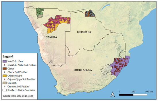
Figure 1.
Areas of interest (AOI) and soil organic carbon in situ data. Own source.

Table 1.
Number of soil profiles and data sources for each region.
Complementary data were sourced from the World Inventory of Soil Emission Potentials (WISE), which offers harmonized point and grid-based soil databases compiled between 1991 and 2016. The WISE dataset includes representative profiles aligned with FAO soil units and enables the estimation of various soil properties such as organic carbon, nitrogen, pH, cation exchange capacity, and texture fractions. These values were then linked to spatial data from the FAO Soil Map of the World to bridge gaps left by other systems such as SOTER [34].
The Soil and Terrain Database (SOTER), developed through collaboration between FAO, UNEP, and ISRIC, provided additional spatial soil information. Although a global SOTER database was never fully completed, regional versions have been compiled for specific countries and continents, offering detailed pedological and topographic data [35].
At a more local scale, important data were extracted from Namibia’s efforts under the Land Degradation Neutrality (LDN) program. As a pilot country, Namibia developed SOC baselines for the Otjozondjupa and Omusati regions, collecting more than 300 field samples according to digital soil mapping methodologies, using a directed stratified sampling design (Table 1). Each location contained four subplots, one central plot, and three peripheral subplots equally distributed along the perimeter of a 5 to 6 m radius circle [36]. Then, soil samples were extracted from the first 20–30 cm using a soil auger. Soil samples were analyzed for dry mass and SOC using the Walkley–Black method [36]. These data not only served to assess SOC stocks but also to establish indicators related to land cover changes and bush encroachment trends [36].
Additional soil observations were made using the National Cooperative Soil Survey (NCSS) of the United States, a long-standing federal initiative focused on soil classification, inventory, and mapping. While primarily focused on the US, the methodological consistency and extensive metadata of NCSS samples offered a valuable comparative input for our modeling framework. However, due to the large area covered by these countries and the large number of protected or inaccessible areas, many areas are not represented by sampling, which will lead to uncertainty in the models for these areas.
Finally, region-specific data from the SteamBioAfrica project played a central role in refining the model calibration for the Otjozondjupa region. During this project, systematic field campaigns and laboratory analyses were conducted in Namibia, Botswana, and South Africa (Figure 1), supporting both the accuracy of our predictions and the alignment of the study with current land-use challenges in southern African savannas (SteamBioAfrica, GA: 101036401). Similar to the studies carried out in Otjozondjupa and Omusati, different replicates were carried out to improve the representativeness of each point sampled in the first 30 cm of soil. The Walkley–Black method was used as the laboratory method to estimate the SOC.
2.2. Study Areas
The regions selected for this study are located across southern Africa, specifically in Namibia, Botswana, and South Africa. The identification of these areas of interest was guided by three key considerations that directly influence the reliability and applicability of digital soil mapping (DSM) efforts.
First, the availability and distribution of field data were a primary factor. High-quality digital soil modeling is contingent upon the accessibility of georeferenced, well-distributed sampling data that capture the natural variability of the parameter under study. By focusing on areas with adequate sampling density, the models would be better equipped to learn from the input data, producing more accurate and spatially robust outputs.
Second, environmental characteristics played a central role in guiding the selection. Much of southern Africa is typified by arid and semi-arid climates, where soils tend to exhibit low organic carbon levels. Despite this general trend, specific regions within these climatic zones display marked variability in soil composition and carbon content, driven by microclimatic, geomorphological, and land-use differences. Targeting such zones allows for a more nuanced understanding of carbon dynamics and improves the capacity of DSM tools to model these patterns under varying environmental conditions.
Finally, practical sampling experience gathered through the SteamBioAfrica project was essential in delineating the study areas. Field campaigns conducted primarily in Otjozondjupa, Namibia, provided critical in situ information that informed both the selection of modelling zones and the calibration of input variables (Figure 2). These efforts facilitated a ground-truth framework for model validation and supported the development of regionally relevant SOC distribution maps, contributing to the broader understanding of carbon sequestration potential across savanna landscapes.
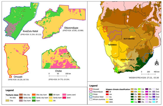
Figure 2.
Areas of interest. Soil texture and Köppen climate classifications. Af—equatorial rainforest; Am—monsoon; Aw—tropical savanna; BWk—cold desert; BWh—hot desert; BSk—cold semi-arid; BSh—hot semi-arid; Cfa—humid subtropical (no dry season, hot summer); Cfb—oceanic (no dry season, warm summer); Cfc—subpolar oceanic; Csa—Mediterranean (dry, hot summer); Csb—Mediterranean (dry, warm summer); Csc—Mediterranean (dry, cold summer); Cwa—subtropical (dry winter, hot summer); Cwb—subtropical (dry winter, warm summer); Cwc—subtropical highland (dry winter, cold summer); Dfa—continental (no dry season, hot summer); Dfb—continental (no dry season, warm summer); Dfc—subarctic (no dry season, cold summer); Dfd—extremely cold subarctic; Dsa—continental (dry summer, hot); Dsb—continental (dry summer, warm); Dsc—continental (dry summer, cold); Dsd—continental (dry summer, extremely cold); Dwa, Dwb, Dwc, Dwd—continental (dry winter variants); EF—ice cap; ET—tundra. Own source.
The study regions encompass a range of climatic zones and soil types that reflect the environmental heterogeneity of southern Africa (Figure 2). These differences play a crucial role in shaping the spatial distribution of soil organic carbon and offer an excellent testbed for evaluating the performance of digital soil mapping approaches across varying biophysical conditions.
In Namibia, the Otjozondjupa and Omusati regions exhibit distinct environmental characteristics. Otjozondjupa lies in a semi-arid to arid zone (BWh-BSh), with average annual rainfall ranging between 300 and 500 mm, highly variable and concentrated during the austral summer months. Soils in this region are often classified as Arenosols and Cambisols (Table 2) [37], typically sandy in texture, with low clay content and limited organic matter (Figure 1). The landscape includes extensive areas of shrubland and degraded savannas, where bush encroachment is a dominant land-use concern [38]. These conditions present both a challenge and an opportunity for mapping soil carbon, as spatial variability is strongly linked to microtopography and localized vegetation patterns.
Table 2.
Summary of case studies—environmental information.
Omusati, situated further northwest, is characterized by even more hot arid conditions (BSh), receiving less than 300 mm of rainfall per year in some areas. The soils are predominantly Regosols and Leptosols [37], often shallow and highly susceptible to erosion. However, floodplains and ephemeral river systems create zones of more fertile soils—such as Fluvisols—where subsistence agriculture is practiced. The heterogeneity within this dryland environment demands high-resolution spatial modeling to capture carbon gradients effectively (Table 2).
The Chobe region in northern Botswana is influenced by a subtropical climate (BSh influenced by Cwb), with higher precipitation compared to Namibia, up to 800 mm annually in some zones. This area includes a mix of Kalahari sands, Ferralsols, and Acrisols [37], particularly in the forested areas near the Chobe River (Table 2). Soil development here is strongly influenced by parent material and seasonal waterlogging, which can enhance organic matter accumulation in specific lowland pockets. The coexistence of dry upland soils and wetter riparian zones adds complexity to SOC modeling.
KwaZulu-Natal in eastern South Africa represents the most mesic environment in the study, with a subtropical to temperate climate (Figure 1; Cfb, Cfa, Cwb, and Cwa) and annual rainfall often exceeding 1000 mm in mountainous areas. The region is known for its fertile soils—such as Nitisols, Luvisols, and Ferralsols [37]—developed under higher rainfall and vegetative productivity (Table 2). These conditions favor higher SOC content and more stable soil structure. However, the variation in topography, from coastal plains to highlands, introduces substantial spatial heterogeneity. This complexity, combined with intensive land use (e.g., forestry, sugarcane, and subsistence agriculture), makes KwaZulu-Natal a critical region for testing the scalability and transferability of machine learning-based SOC prediction models.
These climatic and edaphic contrasts among the selected study areas reinforce the necessity of incorporating diverse environmental variables into the modeling framework and validate the need for region-specific calibration strategies in digital soil mapping.
2.3. Input Variables
To model the spatial distribution of soil organic carbon (SOC), three distinct categories of predictor variables were selected, each closely associated with topsoil characteristics and environmental drivers known to influence carbon dynamics [2,39,40]. These variable groups (topographical, spectral, and climatic) were strategically combined to build and compare model configurations. The first group included topographical variables derived from digital elevation models, namely, elevation, slope, aspect, and the Topographic Wetness Index (TWI). These parameters capture terrain-driven influences on soil formation and moisture redistribution, which are closely linked to organic matter accumulation and decomposition rates [17]
The second group comprised spectral indices derived from Sentinel-2 multispectral imagery. This included vegetation-related indices such as NDVI and GNDVI; brightness and water-related indices; and specific bands known for their relevance to soil surface conditions, notably B11 (shortwave infrared) and B8 (near-infrared). These inputs help quantify vegetation cover, surface reflectance, and moisture content—factors indirectly related to SOC [15,17].
Lastly, the third group incorporates climatic and biophysical variables. These include land surface temperature, annual precipitation, relative humidity, and surface radiance, which reflect local climatic conditions influencing organic matter turnover. Additionally, productivity-related metrics like net primary production (NPP) provide an integrative view of vegetation–soil interactions, essential for assessing the carbon inputs to the soil system [17,40].
These variables were grouped in blocks because different model configurations were defined depending on the combination of variable groups used (Figure 3). Three main configurations were tested: Model A integrated climatic, topographical, and spectral variables; Model B combined topographical and spectral data; and Model C relied solely on spectral indices. This structured approach allowed us to assess the individual and combined contributions of each variable group to SOC prediction accuracy.
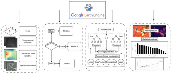
Figure 3.
Schematic diagram of methodology. Using Google Earth Engine, all variables were extracted except for the training dataset. Three Random Forest model configurations were defined, along with their corresponding parameterisation. This process ultimately yielded two main outputs: the raster map of standard deviation and the spatial distribution of soil organic carbon. Own source.
2.3.1. Topographical Variables
Topographic features (Table 3) were derived primarily from the digital elevation model of the NASA Shuttle Radar Topography Mission (SRTM) at a resolution of 30 m. The SRTM V3 product (also known as SRTM Plus), provided by the NASA Jet Propulsion Laboratory, offers near-global coverage and was preprocessed to fill voids using open access datasets such as ASTER GDEM2, GMTED2010, and NED [41]. This dataset serves as the foundation for calculating several terrain-related variables critical to understanding spatial patterns in soil organic carbon (SOC).
Table 3.
Summary table of the topographical variables used to test the model.
From the SRTM DEM, three key derivatives were computed: elevation, slope, and aspect. These were generated using a publicly available processing module within the Google Earth Engine environment, which includes the necessary mathematical expressions to derive such metrics. Elevation is a primary descriptor of landscape position, while slope and aspect influence soil moisture retention, erosion processes, and solar exposure—all of which are indirectly linked to carbon cycling in soils.
Additionally, the Topographic Wetness Index (TWI) was calculated, which integrates local upslope contributing area and slope to identify potential zones of water accumulation or sustained soil moisture. The TWI is particularly useful in semi-arid environments where water redistribution plays a significant role in controlling vegetation patterns and soil organic matter dynamics. Its computation relied on both the slope and flow accumulation layers derived from the DEM, allowing us to represent spatial hydrological processes relevant to SOC modeling.
2.3.2. Climate Variables and Others
To complement the topographic and spectral predictors, a set of climatic and productivity-related variables was incorporated into the modeling framework to account for environmental factors that influence SOC accumulation and distribution (Table 4). These variables, derived from remote sensing products and climate models, were processed through a standard statistics function to extract summary metrics over a predefined temporal range. This temporal aggregation ensured that the predictors captured stable patterns rather than short-term variability, which is critical for improving the robustness of spatial models.
Table 4.
Summary table with the climate data used to test the model.
Among the climate variables tested, land surface temperature (LST) was included due to its strong relationship with SOC dynamics, especially in arid and semi-arid environments. Two datasets were evaluated, namely, the WorldClim climatology and the MOD11A2.061 Terra MODIS LST product, which provides 8-day composites at 1 km resolution. The latter was selected for final modeling, as it has shown better correlations with SOC in previous studies [2,42].
Precipitation data were obtained from the Climate Hazards Group InfraRed Precipitation with Stations (CHIRPS) dataset, which offers over 30 years of quasi-global rainfall estimates at 0.05° resolution. The CHIRPS integrates satellite observations with ground-based meteorological data, producing temporally consistent rainfall time series that are particularly suitable for drought monitoring and long-term trend analysis [43]. Relative humidity (RH) data were sourced from the Global Forecast System (GFS) 384 h predicted atmospheric fields, specifically the “relative_humidity_2m_above_ground (RH)” variable. While initially included in preliminary model testing, RH was excluded from the final configurations due to its coarse spatial resolution, which limited its usefulness for fine-scale SOC prediction.
Downward surface radiance, expressed as downward shortwave radiation (DSR), was included from the MODIS MCD18A1 V6.1 product, which delivers daily estimates at 1 km resolution. DSR reflects the amount of incoming solar radiation across the shortwave spectrum (300–4000 nm), a key input for photosynthetic activity and soil temperature regulation [44].
To account for vegetation productivity and associated organic inputs to the soil, the MOD17A3HGF V6.1 product was tested. This dataset provides annual net primary production (NPP) at 500 m resolution. NPP is computed from 8-day net photosynthesis (PSN) values and represents the net carbon fixed by vegetation after maintenance respiration. Although highly informative, NPP was ultimately replaced by the actual evapotranspiration and interception (ETIa) variable from FAO’s WaPOR platform, which offered finer spatial resolution (250 m) and similar ecological meaning. ETIa combines evaporation, transpiration, and interception losses and is considered a reliable indicator of ecosystem functioning and vegetation–water interactions in dryland contexts.
2.3.3. Spectral Indexes
All spectral information used for SOC modeling was extracted from the Sentinel-2 surface reflectance product (COPERNICUS/S2_SR) for the period 2019 to 2022, applying a cloud cover threshold of 10%. This temporal range allowed for the identification of consistent surface reflectance patterns and seasonal spectral trends across the study areas. The resulting dataset, composed of between 1000 and 5000 image tiles depending on the region, represents a significant volume of data, especially for large and environmentally diverse areas such as Otjozondjupa and KwaZulu-Natal.
Sentinel-2 is a high-resolution, wide-swath, multispectral satellite mission developed under the European Copernicus Program. It provides regular and detailed observations of Earth’s surface, including vegetation, soil, water bodies, and coastal zones. The system acquires data in up to 13 spectral bands (B1 to B12), which serve as the basis for calculating a wide variety of spectral indices relevant to land monitoring applications (Table 5).
Table 5.
Summary table of spectral information used to test the model.
For SOC prediction, a series of spectral indices were derived and categorized into three functional groups based on their ecological relevance and common uses in the remote sensing field. Vegetation-related indices—such as the Normalized Difference Vegetation Index (NDVI), the Enhanced Vegetation Index (EVI), and the Green Normalized Difference Vegetation Index (GNDVI)—were used to quantify vegetation density, chlorophyll activity, and overall plant productivity, which are key contributors to organic matter input to the soil.
Moisture-sensitive indices, including the Moisture Stress Index (MSI) and the Normalized Difference Moisture Index (NDMI), were included to capture the influence of soil and canopy water content. These variables are important for understanding microbial activity and organic matter decomposition, both of which directly affect SOC levels.
Brightness-related indices such as the Brightness Index (BI) and the Soil Organic Carbon Index (SOCI) were incorporated to assess variations in surface reflectance, especially in sparsely vegetated or bare areas. These indices have shown potential for estimating SOC directly from soil surface properties under low vegetation cover.
This set of spectral variables (Table 3) was carefully chosen according to the intrinsic relationship of the variable itself to the ecological meaning of carbon sequestration and storage. In addition, the selection was also based on models and results from other studies [15,40,42].
2.4. Model Configuration
Digital soil mapping requires robust predictive frameworks capable of modeling complex, non-linear relationships among environmental variables while also ensuring generalizability across diverse landscapes. In this study, the random forest (RF) algorithm was selected as the core machine learning model due to its strong performance in ecological and environmental modeling contexts, its capacity to manage high-dimensional datasets, and its resilience to overfitting.
Random forest is an ensemble learning method that operates by constructing a multitude of decision trees during training and outputting the average prediction of individual trees in the case of regression tasks [45,46]. Each tree is trained on a bootstrap sample of the data, and at each node, a random subset of predictors is used to determine the best split (Figure 4). This combination of bagging and feature randomness enhances prediction accuracy and controls model variance. Importantly, RF makes no assumptions about data distributions, making it particularly suitable for heterogeneous and noisy datasets such as those derived from remote sensing and field-based soil observations.
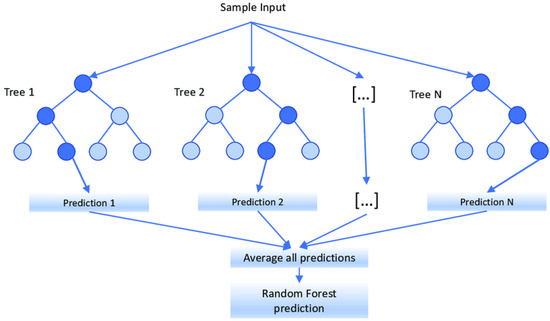
Figure 4.
Random forest scheme [47].
Compared to other machine learning models commonly used in digital soil mapping—such as support vector machines (SVMs), artificial neural networks (ANNs), gradient boosted trees (e.g., XGBoosts), and quantile regression forests (QRFs)—RF provides a favorable balance between accuracy, computational efficiency, and interpretability [48,49,50]. While SVMs and ANNs can yield high predictive performance, they often require extensive parameter tuning and are sensitive to data scaling, and their interpretability is limited. RF, on the other hand, offers variable importance measures that help identify which environmental factors most influence SOC distribution, adding ecological meaning to the results [48,49,50].
To explore how different types of environmental predictors influenced the estimation of soil organic carbon (SOC), three alternative model configurations were developed and tested. Each configuration drew on a distinct combination of variable groups—namely, topographic, spectral, and climatic—allowing us to assess the relative contribution of each to model performance.
The most comprehensive configuration, referred to as Model A, integrated the full set of available predictors, including climate variables (such as temperature and precipitation), topographic parameters (elevation, slope, aspect, and TWI), and spectral indices derived from Sentinel-2 imagery. This model served as a benchmark for evaluating the highest predictive performance attainable when leveraging all environmental data sources.
Model B simplified the predictor set by excluding climate variables, relying instead on topographic and spectral information. This intermediate configuration tested the capacity of landscape structure and surface reflectance data to explain SOC variability without the influence of dynamic climatic factors.
Finally, Model C adopted a more minimalist approach, using only spectral indices derived from Sentinel-2 data. By relying exclusively on Earth observation imagery, this model presented the lowest-data scenario, offering insights into the feasibility of predicting SOC in data-scarce regions using freely available remote sensing products alone.
To ensure that the predictive models were not compromised by multicollinearity, a correlation matrix was computed to examine the degree of linear association between predictor variables (Figure 5). This step was essential for identifying and eliminating redundant information that could distort the estimation of variable importance and reduce the interpretability of the models. Variables exhibiting high pairwise correlations (greater than 0.80/−0.80) were systematically removed to avoid overlapping information content and to reduce the risk of overfitting. By retaining only the most informative and independent predictors, the modeling framework aimed to remain both parsimonious and robust, better suited for extrapolation and spatial prediction of SOC across heterogeneous landscapes. As a reference for this variable selection process, the dataset from Otjozondjupa (the region with the highest number of SOC sampling points) was used to define a consistent and optimized predictor set applicable across all study regions.
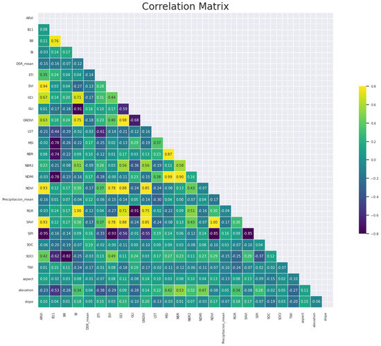
Figure 5.
Correlation matrix used to identify redundancy among predictor variables. Own source.
All models were trained using a random 70/30 split of the SOC dataset into training and validation sets. Between 240 and 580 decision trees were applied for each model, with a minimum leaf population of 5 and several variables per split equal to the square root of the total number of predictors. Trees were grown to full depth (i.e., without maximum node limits) to allow for comprehensive feature space exploration [46]. An out-of-bag (OOB) error analysis was conducted to determine the optimal number of trees (Figure 6). The results indicated that model performance stabilized within the range of 200 to 580 trees across regions. Based on this analysis, a final configuration of ntrees = 500 (default) was selected, as it consistently minimized prediction error. In addition, the bagFraction parameter varied between 0.5 and 1.0 to reduce RMSE and MAE while preventing overfitting. A bagFraction value of 0.8 was ultimately chosen, providing an optimal balance between accuracy and generalizability. The models were evaluated using standard regression performance metrics: coefficient of determination (R2), standard deviation (STD), root mean square error (RMSE), and mean absolute error (MAE).
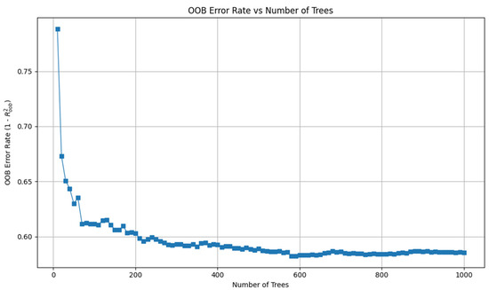
Figure 6.
OOB error analysis to determine the most optimized ntree parameter for the Otjozondjupa region. Own source.
The standard deviation served as a key indicator of the spatial variability and reliability of model predictions. High standard deviation values reflected greater heterogeneity in predicted SOC values across the landscape, whereas low values indicated more consistent and spatially homogeneous predictions. This helped assess the robustness of model outputs and their suitability for spatial planning and management applications. The coefficient of determination (R2) was used to measure the proportion of the variance in observed SOC that was explained by the model predictions. As a measure of goodness of fit, it provided insight into the overall explanatory power of each model configuration. RMSE (root mean square error) was calculated to quantify the average magnitude of prediction error, giving more weight to larger errors. It was computed as the square root of the mean of squared differences between predicted and observed values, serving as a measure of error dispersion. Finally, MAE (mean absolute error), on the other hand, provided a more interpretable metric by averaging the absolute differences between predicted and observed SOC values, regardless of direction. This index is particularly useful when a straightforward understanding of the model’s average error is needed.
The entire modeling process was conducted within the Google Earth Engine (GEE) platform using JavaScript. GEE is a cloud-based geospatial processing environment optimized for large-scale environmental data handling. Its integration with planetary-scale datasets such as Sentinel-2, MODIS, and CHIRPS allowed us to manage, preprocess, and analyze massive multi-temporal datasets efficiently. The use of cloud computing was essential given the high volume of image tiles (ranging from 1000 to over 5000 per region), which would be difficult to process with conventional desktop systems. JavaScript scripting in GEE facilitated rapid implementation of the random forest algorithm, with distributed computation allowing model training over large and data-rich regions such as Otjozondjupa and KwaZulu-Natal.
3. Results
3.1. Statistical Analysis of SOC
The descriptive analysis of soil organic carbon (SOC) across the study regions revealed notable differences in both mean values and variability (Table 6). In the Otjozondjupa region, the mean SOC was 4.16 g/kg, with a standard deviation (STD) of 2.64 and a coefficient of variation (CV) of 0.634, indicating moderate variability and a relatively consistent SOC distribution. The Chobe region displayed a higher mean SOC of 4.47 g/kg, with a wider range (1 to 38 g/kg), and greater variability (STD: 4.06, CV: 0.908), suggesting a more heterogeneous distribution of organic carbon values.
Table 6.
Descriptive statistical analysis of the soil organic carbon. AOI—area of interest; N—samples; S.D.—standard deviation; CV—coefficient of variation. The table presents a descriptive statistical analysis of soil organic carbon (SOC) data across four areas of interest (AOI): Otjozondjupa, Chobe, Omusati, and KwaZulu-Natal. The parameters include the number of samples (N), minimum and maximum SOC values, mean, coefficient of variation (CV), and standard deviation (STD).
In contrast, Omusati recorded the lowest mean SOC value (2.54 g/kg), with an STD of 1.73 and a CV of 0.682, reflecting moderate variability and generally lower carbon content. The KwaZulu-Natal region exhibited the highest SOC mean at 9.58 g/kg, and the broadest range of values (1 to 42 g/kg), accompanied by high variability (STD: 8.41, CV: 0.878), consistent with significant spatial heterogeneity.
Aggregated across all study sites, the overall mean SOC value was 4.91 g/kg, with a high CV of 1.016 and a STD of 4.99, highlighting pronounced variability among regions. These results illustrate the spatial heterogeneity of SOC in southern Africa and indicate the influence of regional conditions on SOC distribution patterns.
3.2. Spatial Model Performance
As previously indicated, lines of code were specified throughout that reflected different model performance indicators, which are detailed by model and region in the Table 7 and Figure 7
Table 7.
Results of model performance indicators in the different regions.
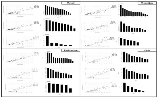
Figure 7.
Scatter plots and variable importance histograms per model configuration and region.
The model reliability indicator values showed highly disparate results among regions as well as models (Table 7). It was observed that Model A exhibited the best performance, accounting for 78% (R2 of 0.78) of the spatial variation in SOC in the Otjozondjupa region. Generally, a higher number of predictors contributes to better model performance. Model A incorporated 14 predictive variables, including multispectral remote sensing, topographic, and climatic variables. Model B, focusing on topographic and spectral information, resulted in a maximum R2 of 0.77 and an RMSE of 1.18 g/kg SOC in Otjozondjupa. Conversely, Model C, solely relying on multispectral remote sensing-derived variables, also resulted in an R2 of 0.73 and an RMSE of 1.36 g/kg in Otjozondjupa.
Omusati was the second region where the model performance indicators yielded the best results, with a maximum R2 of 0.74 for Model A and an RMSE of 1.31 g/kg. Model B produced the lowest RMSE (1.2) and MAE (0.79), despite having a lower R2 than Model A (Table 7, indicating that Model B provided more accurate predictions in terms of absolute error. In KwaZulu-Natal, RMSE values reached up to 6.72 g/kg, indicating considerable error primarily due to the broad range of SOC values in the region. High MAE values were also recorded, up to 5.43 for Model C (Table 7).
Similar findings were observed in the Chobe region, where the lowest R2 value among the models was recorded—0.62 for Model B, with an RMSE of 2.93 and an MAE of 1.69—resulting in the least optimal performance for SOC prediction (Table 5). In this region, the sampling point distribution was limited and inadequate for digital soil mapping purposes. Although many points existed, their poor spatial distribution left many areas without coverage. Moreover, the quality of the data was questionable; they were seemingly inaccurate and derived from somewhat old databases, which diminished their reliability. As previously described, Otjozondjupa benefited from a well-structured soil sampling design, which aligned effectively with digital soil mapping using machine learning algorithms. These findings confirmed that Otjozondjupa had the most favorable data conditions for SOC prediction in the context of this study.
The soil organic carbon (SOC) predictions in KwaZulu-Natal (Figure 8) showed similar behavior across the three model configurations. Models B and C were very similar, displaying higher SOC values compared to Model A. The west-central area had the lowest SOC, corresponding with a lower standard deviation, which indicates higher prediction reliability in that region. The highest SOC values were concentrated in the wooded and mountainous areas bordering Lesotho, as well as throughout the southern part of the region. The lowest reliability values were found along the entire eastern coast of the region, especially for Model A. The results obtained for this region were consistent with those of other models previously conducted in the area [40,50], particularly in areas with the lowest carbon predictions, where bush encroachment is more likely due to climatic conditions.
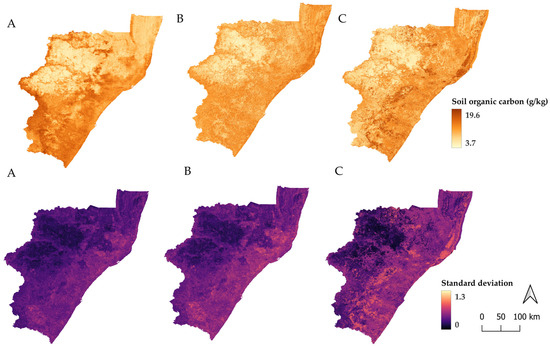
Figure 8.
Predicted soil organic carbon (SOC) distribution (0–20 cm) and associated standard deviation in KwaZulu-Natal using three model configurations. At the top, the mean SOC predictions (g/kg) generated by Model A (full predictor set), Model B (excluding climate variables), and Model C (spectral indices only) are illustrated. At the bottom, the corresponding prediction uncertainty expressed as the standard deviation of the random forest ensemble is shown.
The SOC predictions for the Otjozondjupa region showed certain differences among the three models (Figure 9). The most notable difference was that Models B and C again overestimated the SOC value compared to Model A. In areas such as the extreme east, the predictions of Models B and C were higher than those of Model A. In the northwest areas of the region, this same pattern was evident. When comparing our results with other known sources such as SoilsGrid [51], ISDAsoil [40], or even the model developed after the planned sampling in the area [36], it was observed that Model A showed the most similarities and achieved the best statistical results among all the models, but Models B and C also yielded very similar results.
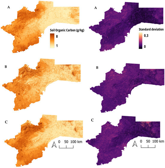
Figure 9.
Predicted soil organic carbon (SOC) distribution (0–20 cm) and associated standard deviation in Otjozondjupa using three model configurations. On the left side, the mean SOC predictions (g/kg) generated by Model A (full predictor set), Model B (excluding climate variables), and Model C (spectral indices only) are illustrated. On the right side, the corresponding prediction uncertainty expressed as the standard deviation of the random forest ensemble is shown.
This region, like Otjozondjupa, had data points well distributed spatially, which explains why it was the second region with the best mapping and SOC prediction results (Figure 10). In this region, the opposite was observed as in the previous ones; in this case, Model A presented an SOC prediction with higher values than Models B and C. In the northwest and south, in particular, the predictions were the highest in the region. The SD values were higher in Model A than in Models B and C in these areas. On the other hand, Model A yielded better SD results in the north and southwest of Omusati. The outputs were very similar to other prediction maps [40,50].
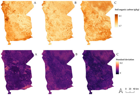
Figure 10.
Predicted soil organic carbon (SOC) distribution (0–20 cm) and associated standard deviation in Omusati using three model configurations. At the top, the mean SOC predictions (g/kg) generated by Model A (full predictor set), Model B (excluding climate variables), and Model C (spectral indices only) are illustrated. At the bottom, the corresponding prediction uncertainty expressed as the standard deviation of the random forest ensemble is shown.
Finally, for Chobe, we obtained quite similar results among the different models (Figure 11). The areas with higher carbon values were the same in all models, although Model A showed slightly higher values than Models B and C. Additionally, in the central part of Chobe, Model A highlighted areas of higher carbon that were not captured by Models B and C. However, these areas were reflected with considerable uncertainty in the standard deviation maps, with Models B and C showing less uncertainty in much of the central region of Chobe. Compared to other models mentioned, these results were very similar to other soil variable prediction models [40,50].
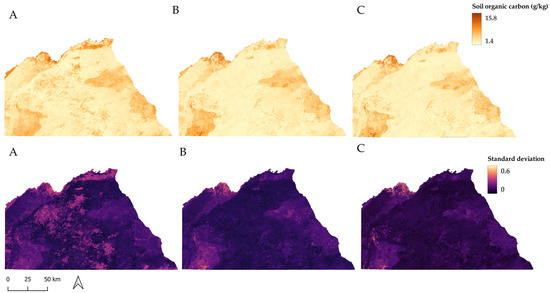
Figure 11.
Predicted soil organic carbon (SOC) distribution (0–20 cm) and associated standard deviation in Chobe using three model configurations. At the top, the mean SOC predictions (g/kg) generated by Model A (full predictor set), Model B (excluding climate variables), and Model C (spectral indices only) are illustrated. At the bottom, the corresponding prediction uncertainty expressed as the standard deviation of the random forest ensemble is shown.
4. Discussion
The regional differences observed in SOC values and their associated variability highlight the complex interplay between environmental, topographic, and management-related factors in shaping soil carbon dynamics across southern Africa. In the Otjozondjupa region, a moderate mean SOC value (4.16 g/kg) and low coefficient of variation (CV = 0.634) suggested a relatively homogeneous landscape and a well-structured soil sampling strategy. These characteristics likely contributed to the consistency and reliability of the SOC predictions in this area. In contrast, the Chobe region exhibited a higher mean SOC (4.47 g/kg) but also greater variability (CV = 0.908), with values ranging from 1 to 38 g/kg. This heterogeneity may reflect the coexistence of diverse land uses, soil types, and vegetation structures, which complicate the spatial distribution of SOC.
Omusati, located in a more arid environment, presented the lowest mean SOC value (2.54 g/kg) and moderate variability (CV = 0.682). These results are consistent with the region’s limited vegetation cover, low precipitation levels, and soil types less conducive to carbon accumulation. By contrast, KwaZulu-Natal had the highest mean SOC (9.58 g/kg), with values ranging from 1 to 42 g/kg. The high standard deviation (8.41) and coefficient of variation (0.878) reflect the pronounced heterogeneity of this region, which is characterized by complex topography, diverse vegetation types, and intensive land use. These findings reinforce the need for region-specific analyses and management practices, especially in ecologically diverse or climatically extreme zones.
When considering all regions collectively, the mean SOC value (4.91 g/kg), standard deviation (4.99), and high overall CV (1.016) highlight the substantial heterogeneity of SOC distribution across the study area. This variability emphasizes the need for high-resolution spatial data and localized monitoring efforts to better understand soil functioning and guide sustainable land management.
The key predictors identified across model configurations were in line with previous findings. Surface temperature was negatively associated with SOC content, with higher carbon levels found in cooler areas [50,51]. Elevation was another critical predictor, showing positive correlations with SOC values, particularly in arid regions with elevations between 481 and 3035 m [52,53]. This is consistent with the literature, where topographic variables such as slope, aspect, and elevation have been frequently used as reliable proxies for soil formation processes and organic matter accumulation [54,55,56].
Spectral information also played a crucial role. Sentinel-2 bands B11 (SWIR) and B8 (NIR), along with indices such as BI, GNDVI, and NDMI, were strongly correlated with SOC content. These indices capture vegetation vigor and moisture conditions, both essential for understanding soil organic matter inputs and decomposition rates [15,41]. In Model A, which included climatic, topographic, and spectral variables, the most influential predictors were surface temperature, precipitation, elevation, surface radiance, and B11 reflectance. This combination highlights the need to integrate multisource environmental data to optimize model performance. In Models B and C, where climatic data were excluded, variables such as elevation and vegetation indices remained highly relevant, confirming their predictive power even under data-scarce scenarios.
However, despite the strong predictive capacity of RF, the model’s effectiveness is contingent upon the quality and representativeness of the input data. Notably, regions with better sampling design, such as Otjozondjupa and Omusati, showed more reliable predictions. In contrast, Chobe and KwaZulu-Natal, despite having many data points, suffered from uneven geographic distribution and inconsistencies in sampling methodology. These deficiencies likely contributed to the lower performance metrics and increased prediction uncertainty in those areas. A significant challenge remains the limited availability of harmonized and spatially distributed soil data, particularly in the southern areas of Omusati and parts of Chobe and KwaZulu-Natal. The lack of high-quality training data, combined with the inherent variability of SOC even within short distances, complicates model calibration and validation. Furthermore, differences in sampling depth, laboratory procedures, and geolocation accuracy can introduce additional uncertainty. These factors reinforce the need to expand soil monitoring efforts with standardized protocols and consistent metadata across regions [57].
Finally, in the context of model optimization, we paid particular attention to striking a balance between model complexity and generalizability. While random forests are known for handling high-dimensional data effectively, we acknowledged that incorporating too many predictors—especially in data-scarce regions—could increase the risk of overfitting. To address this, we implemented a variable decorrelation analysis and excluded redundant or low-informative variables from the model. This approach, aligned with recommendations from previous studies [10], aimed to enhance both the stability and interpretability of the predictive models.
In conclusion, this discussion confirms the utility of DSM approaches and RF models for SOC mapping in complex landscapes while also highlighting critical limitations related to data quality and spatial coverage. Future efforts should focus on improving the consistency of soil data, expanding field campaigns in under-represented areas, and leveraging synergies between remote sensing, environmental monitoring, and machine learning to produce more accurate and actionable soil information. Moreover, based on our findings, we recommend a set of predictor variables that balance model accuracy and ecological interpretability. The optimal combination included topographic variables such as elevation and the Topographic Wetness Index (TWI); spectral indices from Sentinel-2—particularly B11 (SWIR), B8 (NIR), GNDVI (a vegetation index), NDMI (a moisture index), and BI (a brightness index); and climatic variables like land surface temperature (LST) and annual precipitation. These variables consistently ranked highest in importance across model configurations and are supported by previous studies for their strong associations with soil formation processes, organic matter dynamics, and vegetation productivity.
5. Conclusions
This study presented significant advances in the spatial modeling of soil organic carbon (SOC) in selected areas of Botswana, Namibia, and South Africa. By merging open-access data with harmonized field observations from project collaborators and applying RF algorithms within the GEE platform, precise and spatially explicit SOC predictions were generated for a variety of semi-arid ecosystems. The approach employed high-resolution remotely sensed data and environmental covariates to construct robust models suitable for large-scale DSM applications. The resulting spatial products provided valuable tools for environmental managers and policymakers, particularly in the context of carbon management strategy planning, biomass utilization, and sustainable land use. Information on the spatial heterogeneity of SOC was shown to be essential for enhancing ecosystem services such as water regulation, carbon sequestration, and soil fertility in vulnerable dryland regions.
One of the key outputs of this research is an open access, reproducible RF model framework run in GEE with supporting coded documentation and explanatory annotation. The facility allows for additional applied analysis and replication elsewhere and promotes transparency and scientific reproducibility of DSM work. The study also highlights the crucial importance of soil data quality: regions such as Otjozondjupa and Omusati, which have had consistent and recent sampling campaigns, had superior SOC estimates. Conversely, regions with sparse and irregular sampling records had higher uncertainty, affirming the necessity of supplementary and harmonized soil surveys in data-scarce regions.
Furthermore, SOC content was also found to vary substantially with land-use change, as afforestation or reforestation boosted SOC stocks, but degradation or land clearing resulted in substantial loss. These observations reinforce the importance of SOC monitoring as it relates to climate change mitigation and land restoration processes. The approach employed in the SteamBioAfrica project provides a reproducible and scalable framework for future activities in SOC mapping for Africa and other semi-arid regions, thus furthering evidence-based decision-making for the use of sustainable biomass, land reclamation, and climate policy development. Unlike previous DSM initiatives such as SoilGrids [41], which primarily rely on static global covariates and legacy data, our approach capitalizes on real-time Sentinel-2 imagery within the GEE environment. This enables dynamic, high-resolution modeling and regionally calibrated predictions, achieving finer spatial detail than many existing global SOC mapping products. Moreover, by publishing the source code and providing clear documentation, we ensure that researchers or practitioners with basic technical knowledge can replicate or adapt the model in any region of interest, provided that relevant SOC field data are available.
To further enhance SOC predictions, especially in poorly sampled areas, future research could explore the integration of Sentinel-1 radar data, Sentinel-3 biophysical products, or regional downscaled climate models. Additionally, upcoming Earth observation missions from the European Space Agency, such as BIOMASS (focused on forest carbon stocks) and FLEX (targeting vegetation fluorescence and photosynthetic activity), may offer valuable inputs to improve the spatial and temporal accuracy of SOC estimates.
Author Contributions
Conceptualization, J.B.-G. and F.J.B.-V.; methodology, J.B.-G.; software, J.B.-G.; validation, J.B.-G., M.A.-R., J.M.C.-N. and F.J.B.-V.; formal analysis, J.M.C.-N.; investigation, J.B.-G.; resources, J.B.-G.; data curation, J.B.-G.; writing—original draft preparation, J.B.-G.; writing—review and editing, M.A.-R. and J.M.C.-N.; visualization, J.B.-G.; supervision, J.M.C.-N., F.J.B.-V. and M.A.-R.; project administration, M.A.-R. All authors have read and agreed to the published version of the manuscript.
Funding
This research was funded by the European Commission through the SteamBioAfrica project, under grant number 101036401.
Data Availability Statement
The data is full available under request through the author mail.
Acknowledgments
We want to thank all the STEAMBIOAFRICA team for their support in writing ideas and project development (STEAMBIOAFRICA project, supported by the European Commission’s Horizon 2020 Program, Grant Agreement ID: 101036401).
Conflicts of Interest
Author Mr. Javier Bravo-Garcia, Dr. Francisco José Blanco-Velázquez and Dr. Maria Anaya-Romero are employed by the company Evenor-Tech (Spain). The remaining authors declare that the research was conducted in the absence of any commercial or financial relationships that could be construed as a potential conflict of interest.
Abbreviations
The following abbreviations are used in this manuscript:
| SOC | Soil organic carbon |
| RF | Random forest |
| DSM | Digital soil mapping |
| GEE | Google Earth Engine |
| CV | Coefficient of variation |
| STD | Standard deviation |
| NDMI | Normalized Difference Moisture Index |
| GNDVI | Green Normalized Difference Vegetation Index |
| BI | Brightness Index |
| SOCI | Soil Organic Carbon Index |
| NBR | Normalized Burn Ratio |
| MSI | Moisture Stress Index |
| SIPI | Structure Insensitive Pigment Index |
| DEM | Digital elevation model |
| QRF | Quantile regression forest |
| ANN | Artificial neural network |
| SVM | Support vector machine |
| RMSE | Root mean square error |
| MAE | Mean absolute error |
References
- Lehmann, J.; Bossio, D.A.; Kögel-Knabner, I.; Rillig, M.C. The concept and future prospects of soil health. Nat. Rev. Earth Environ. 2020, 1, 544–553. [Google Scholar] [CrossRef] [PubMed]
- Aji, M.B.W.; Ghozali, A. Environmental carrying capacity based on ecosystem services of Penajam Paser Utara Regency. IOP Conf. Ser. Earth Environ. Sci. 2020, 447, 012062. [Google Scholar] [CrossRef]
- Lal, R. Soil carbon sequestration to mitigate climate change. Geoderma 2004, 123, 1–22. [Google Scholar] [CrossRef]
- Villat, J.; Nicholas, K.A. Quantifying soil carbon sequestration from regenerative agricultural practices in crops and vineyards. Front. Sustain. Food Syst. 2024, 7, 1234108. [Google Scholar] [CrossRef]
- Smith, P.; Soussana, J.; Angers, D.; Schipper, L.; Chenu, C.; Rasse, D.P.; Batjes, N.H.; Van Egmond, F.; McNeill, S.; Kuhnert, M.; et al. How to measure, report and verify soil carbon change to realize the potential of soil carbon sequestration for atmospheric greenhouse gas removal. Glob. Change Biol. 2016, 26, 219–241. [Google Scholar] [CrossRef]
- IPBES. Thematic Assessment Report on the Underlying Causes of Biodiversity Loss and the Determinants of Transformative Change and Options for Achieving the 2050 Vision for Biodiversity of the Intergovernmental Science-Policy Platform on Biodiversity and Ecosystem Services; O’Brien, K., Garibaldi, L., Agrawal, A., Eds.; IPBES Secretariat: Bonn, Germany, 2024. [Google Scholar] [CrossRef]
- Awala, S.K.; Hove, K.; Wanga, M.A.; Valombola, J.S.; Mwandemele, O.D. Rainfall Trend and Variability in Semi-Arid Northern Namibia: Implications for Smallholder Agricultural Production. Welwitschai Int. J. Agric. Sci. 2019, 1, 1–25. [Google Scholar]
- Shikangalah, R. The 2019 drought in Namibia: An overview. J. Namib. Stud. 2020, 27, 37–58. [Google Scholar]
- Keja-Kaereho, C.; Tjizu, B.R. Climate Change and Global Warming in Namibia: Environmental Disasters vs. Human Life and the Economy. Manag. Econ. Res. J. 2019, 5, 11. [Google Scholar] [CrossRef]
- Meyer, R.; Wright, C.; Rother, H. Assessment of SADC Countries & rsquo; National Adaptation Planning Health Impacts Inclusion: A Thorough Review. Ann. Glob. Health 2024, 90, 57. [Google Scholar] [CrossRef]
- Mendelsohn, J.; Jarvis, A.; Robertson, T.; Mendelsohn, M. Atlas of Namibia-Its Land, Water and Life; Namibia Nature Foundation: Windhoek, Namibia, 2022. [Google Scholar]
- Jones, A.; Breuning-Madsen, H.; Brossard, M.; Dampha, A.; Dewitte, O.; Hallett, S.; Jones, R.; Kilasara, M.; Le Roux, P.; Micheli, E.; et al. Soil Atlas of Africa, EUR 25534 EN; Publications Office of the European Union: Luxembourg, 2013. [Google Scholar]
- Adeniyi, O.D.; Bature, H.; Mearker, M. A Systematic Review on Digital Soil Mapping Approaches in Lowland Areas. Land 2024, 13, 379. [Google Scholar] [CrossRef]
- Velázquez, F.J.B.; Shahabi, M.; Rezaei, H.; González-Peñaloza, F.; Shahbazi, F.; Anaya-Romero, M. The possibility of spatial mapping of SOC content in olive groves under integrated production using easy-to-obtain ancillary data in a Mediterranean area. Open Res. Eur. 2024, 2, 110. [Google Scholar] [CrossRef]
- Gholizadeh, A.; Žižala, D.; Saberioon, M.; Borůvka, L. Soil organic carbon and texture retrieving and mapping using proximal, airborne and Sentinel-2 spectral imaging. Remote Sens. Environ. 2018, 218, 89–103. [Google Scholar] [CrossRef]
- Zomer, R.J.; Bossio, D.A.; Sommer, R.; Verchot, L.V. Global sequestration potential of increased organic carbon in cropland soils. Sci. Rep. 2017, 7, 15554. [Google Scholar] [CrossRef]
- Mitran, T.; Suresh, J.; Sujatha, G.; Sreenivas, K.; Karak, S.; Kumar, R.; Chauhan, P.; Meena, R.S. Digital Soil Mapping: A Tool for Sustainable Soil Management. In Climate Change and Soil-Water-Plant Nexus; Rahman, M.M., Biswas, J.C., Meena, R.S., Eds.; Springer: Singapore, 2024. [Google Scholar] [CrossRef]
- Lima, A.A.J.; Lopes, J.C.; Lopes, R.P.; De Figueiredo, T.; Vidal-Vázquez, E.; Hernández, Z. Soil Organic Carbon Assessment Using Remote-Sensing Data and Machine Learning: A Systematic Literature review. Remote Sens. 2025, 17, 882. [Google Scholar] [CrossRef]
- Shanmugapriya, P.; Rathika, S.; Ramesh, T.; Janaki, P. Applications of Remote Sensing in Agriculture—A Review. Int. J. Curr. Microbiol. Appl. Sci. 2019, 8, 2270–2283. [Google Scholar] [CrossRef]
- Castaldi, F.; Hueni, A.; Chabrillat, S.; Ward, K.; Buttafuoco, G.; Bomans, B.; Vreys, K.; Brell, M.; Van Wesemael, B. Evaluating the capability of the Sentinel 2 data for soil organic carbon prediction in croplands. ISPRS J. Photogramm. Remote Sens. 2018, 147, 267–282. [Google Scholar] [CrossRef]
- Castaldi, F.; Casa, R.; Castrignanò, A.; Pascucci, S.; Palombo, A.; Pignatti, S. Estimation of soil properties at the field scale from satellite data: A comparison between spatial and non-spatial techniques. Eur. J. Soil Sci. 2014, 65, 842–851. [Google Scholar] [CrossRef]
- Li, S.; Rossel Ra, V.; Webster, R. The cost-effectiveness of reflectance spectroscopy for estimating soil organic carbon. Eur. J. Soil Sci. 2021, 73, e13202. [Google Scholar] [CrossRef]
- Grunwald, S.; Thompson, J.A.; Boettinger, J.L. Digital soil mapping and modeling at continental scales: Finding solutions for global issues. Soil Sci. Soc. Am. J. 2011, 75, 1201–1213. [Google Scholar] [CrossRef]
- Nenkam, A.M.; Wadoux, A.M.; Minasny, B.; Silatsa, F.B.; Yemefack, M.; Ugbaje, S.U.; Akpa, S.; Van Zijl, G.; Bouasria, A.; Bouslihim, Y.; et al. Applications and challenges of digital soil mapping in Africa. Geoderma 2024, 449, 117007. [Google Scholar] [CrossRef]
- Pouladi, N.; Gholizadeh, A.; Khosravi, V.; Borůvka, L. Digital mapping of soil organic carbon using remote sensing data: A systematic review. Catena 2023, 232, 107409. [Google Scholar] [CrossRef]
- Cord, A.F.; Brauman, K.A.; Chaplin-Kramer, R.; Huth, A.; Ziv, G.; Seppelt, R. Priorities to advance monitoring of ecosystem services using Earth observation. Trends Ecol. Evol. 2017, 32, 416–428. [Google Scholar] [PubMed]
- Ramirez-Reyes, C.; Brauman, K.A.; Chaplin-Kramer, R.; Galford, G.L.; Adamo, S.B.; Anderson, C.B.; Anderson, C.; Allington, G.R.; Bagstad, K.J.; Coe, M.T.; et al. Reimagining the potential of Earth observations for ecosystem service assessments. Sci. Total Environ. 2019, 665, 1053–1063. [Google Scholar] [CrossRef]
- Radočaj, D.; Gašparović, M.; Jurišić, M. Open Remote Sensing Data in Digital Soil Organic Carbon Mapping: A Review. Agriculture 2024, 14, 1005. [Google Scholar] [CrossRef]
- Venter, Z.S.; Hawkins, H.; Cramer, M.D.; Mills, A.J. Mapping soil organic carbon stocks and trends with satellite-driven high-resolution maps over South Africa. Sci. Total Environ. 2021, 771, 145384. [Google Scholar] [CrossRef]
- Yuzugullu, O.; Fajraoui, N.; Don, A.; Liebisch, F. Satellite-based soil organic carbon mapping on European soils using available datasets and support sampling. Sci. Remote Sens. 2024, 9, 100118. [Google Scholar] [CrossRef]
- Abbasi, R.; Martinez, P.; Ahmad, R. The digitization of agricultural industry—A systematic literature review on agriculture 4.0. Smart Agric. Technol. 2022, 2, 100042. [Google Scholar] [CrossRef]
- Batjes, N.H.; Ribeiro, E.; van Oostrum, A.; Leenaars, J.G.B.; Hengl, T.; de Jesus, J.M. WoSIS: Providing standardised soil profile data for the world. Earth Syst. Sci. Data 2020, 12, 299–320. [Google Scholar] [CrossRef]
- Leenaars, J.G.B.; Claessens, L.; Heuvelink, G.B.M.; Hengl, T.; Gonzalez, M.R.; van Bussel, L.G.J. Mapping rootable depth and root zone plant-available water holding capacity of the soil of sub-Saharan Africa. Geoderma 2014, 324, 18–33. [Google Scholar] [CrossRef]
- Batjes, N.H. Harmonized soil property values for broad-scale modelling (WISE30sec) with estimates of global soil carbon stocks. Geoderma 2016, 269, 61–68. [Google Scholar] [CrossRef]
- Van Engelen, V.W.P.; Dijkshoorn, J.A. Global and National Soils and Terrain Databases (SOTER): Procedures Manual (Versión 2.0); ISRIC—World Soil Information: Wageningen, The Netherlands, 2013; Available online: https://www.isric.org/sites/default/files/isric_report_2013_04.pdf (accessed on 15 June 2025).
- Nijbroek, R.; Piikki, K.; Söderström, M.; Kempen, B.; Turner, K.; Hengari, S.; Mutua, J. Soil Organic Carbon Baselines for Land Degradation Neutrality: Map Accuracy and Cost Tradeoffs with Respect to Complexity in Otjozondjupa, Namibia. Sustainability 2018, 10, 1610. [Google Scholar] [CrossRef]
- IUSS Working Group WRB. World Reference Base for Soil Resources. In International Soil Classification System for Naming Soils and Creating Legends for Soil Maps, 4th ed.; International Union of Soil Sciences (IUSS): Vienna, Austria, 2022. [Google Scholar]
- Bravo-García, J.; Camarillo-Naranjo, J.; Blanco-Velázquez, F.J.; González-Peñaloza, F.; Anaya-Romero, M. Mapping the potential habitat suitability and opportunities of bush encroacher species in Southern Africa: A case study of the SteamBioAfrica project. Front. Biogeogr. 2024, 17, e136222. [Google Scholar] [CrossRef]
- Mitran, T.; Suresh, J.; Sujatha, G.; Kandrika, S.; Karak, S.; Kumar, R.; Chauhan, P.; Meena, R. Digital soil mapping of soil properties using Sentinel-2 and topographic variables. Remote Sens. 2020, 12, 3783. [Google Scholar] [CrossRef]
- Miller, M.A.E.; Shepherd, K.D.; Kisitu, B.; Collinson, J. iSDAsoil: The first continent-scale soil property map at 30 m resolution provides a soil information revolution for Africa. PLoS Biol. 2021, 19, e3001441. [Google Scholar] [CrossRef]
- Duarte, E.; Zagal, E.; Barrera, J.A.; Dube, F.; Casco, F.; Hernández, A.J. Digital mapping of soil organic carbon stocks in the forest lands of Dominican Republic. Eur. J. Remote Sens. 2022, 55, 213–231. [Google Scholar] [CrossRef]
- Farr, T.G.; Hensley, S.; Rodriguez, E.; Martin, J.; Kobrick, M. The Shuttle Radar Topography Mission. Rev. Geophys. 2007, 45, RG2004. [Google Scholar] [CrossRef]
- Poggio, L.; De Sousa, L.M.; Batjes, N.H.; Heuvelink, G.B.M.; Kempen, B.; Ribeiro, E.; Rossiter, D. SoilGrids 2.0: Producing soil information for the globe with quantified spatial uncertainty. Soil 2021, 7, 217–240. [Google Scholar] [CrossRef]
- Funk, C.; Peterson, P.; Landsfeld, M.; Pedreros, D.; Verdin, J.; Shukla, S.; Husak, G.; Rowland, J.; Harrison, L.; Hoell, A.; et al. The climate hazards infrared precipitation with stations—A new environmental record for monitoring extremes. Sci. Data 2015, 2, 150066. [Google Scholar] [CrossRef] [PubMed]
- Wang, S. MODIS Downward Shortwave Radiation: User Guide for MCD18A1 V6.1.; NASA MODIS Land Science Team Documentation. 2022. Available online: https://lpdaac.usgs.gov/documents/1658/MCD18_User_Guide_V62.pdf (accessed on 15 June 2025).
- Breiman, L. Random Forests. Mach. Learn. 2001, 45, 5–32. [Google Scholar] [CrossRef]
- Grimm, R.; Behrens, T.; Märker, M.; Elsenbeer, H. Soil organic carbon concentrations and stocks on Barro Colorado Island—Digital soil mapping using Random Forests analysis. Geoderma 2008, 146, 102–113. [Google Scholar] [CrossRef]
- Alzahrani, A.A. Predicting Market Risk Using Machine Learning: A Comparative Analysis of SVM, Random Forest, and Gradient Boosting Algorithms. Go Far AI. 2022. Available online: https://www.gofar.ai/p/predicting-market-risk-using-machine (accessed on 25 June 2025).
- Wadoux, A.M.; Minasny, B.; McBratney, A.B. Machine learning for digital soil mapping: Applications, challenges and suggested solutions. Earth-Sci. Rev. 2020, 210, 103359. [Google Scholar] [CrossRef]
- Hengl, T.; Heuvelink, G.B.M.; Kempen, B.; Leenaars, J.G.B.; Walsh, M.G.; Shepherd, K.D.; Sila, A.; MacMillan, R.A.; De Jesus, J.M.; Tamene, L.; et al. Mapping Soil Properties of Africa at 250 m Resolution: Random Forests Significantly Improve Current Predictions. PLoS ONE 2015, 10, e0125814. [Google Scholar] [CrossRef]
- Hengl, T.; De Jesus, J.M.; Heuvelink, G.B.M.; Gonzalez, M.R.; Kilibarda, M.; Blagotić, A.; Shangguan, W.; Wright, M.N.; Geng, X.; Bauer-Marschallinger, B.; et al. SoilGrids250m: Global gridded soil information based on machine learning. PLoS ONE 2017, 12, e0169748. [Google Scholar] [CrossRef]
- Beucher, A.; Møller, A.; Greve, M. Artificial neural networks and decision tree classification for predicting soil drainage classes in Denmark. Geoderma 2017, 352, 351–359. [Google Scholar] [CrossRef]
- Wang, H.; Yin, Y.; Cai, T.; Tian, X.; Chen, Z.; He, K.; Wang, Z.; Gong, H.; Miao, Q.; Wang, Y.; et al. Global patterns of soil organic carbon dynamics in the 20–100 cm soil profile for different ecosystems: A global meta-analysis. Earth Syst. Sci. Data Discuss. 2024. in review. [Google Scholar] [CrossRef]
- Saeed, S.; Sun, Y.; Beckline, M.; Chen, L.; Lai, Z.; Mannan, A.; Ahmad, A.; Shah, S.; Amir, M.; Ullah, T.; et al. Altitudinal gradients and forest edge effect on soil organic carbon in Chinese fir (Cunninghamia lanceolata): A study from southeastern China. Appl. Ecol. Environ. Res. 2019, 17, 745–757. [Google Scholar] [CrossRef]
- Mosleh, M.K.; Hassan, Q.K.; Chowdhury, E.H. Development of a remote sensing-based rice yield forecasting model. Span. J. Agric. Res. 2016, 14, e0907. [Google Scholar] [CrossRef]
- Padarian, J.; McBratney, A.B.; Minasny, B. Game theory interpretation of digital soil mapping convolutional neural networks. Soil 2020, 6, 389–397. [Google Scholar] [CrossRef]
- Odebiri, O.; Mutanga, O.; Odindi, J.; Slotow, R.; Mafongoya, P.; Lottering, R.; Naicker, R.; Matongera, T.N.; Mngadi, M. Mapping sub-surface distribution of soil organic carbon stocks in South Africa’s arid and semi-arid landscapes: Implications for land management and climate change mitigation. Geoderma Reg. 2024, 37, e00817. [Google Scholar] [CrossRef]
Disclaimer/Publisher’s Note: The statements, opinions and data contained in all publications are solely those of the individual author(s) and contributor(s) and not of MDPI and/or the editor(s). MDPI and/or the editor(s) disclaim responsibility for any injury to people or property resulting from any ideas, methods, instructions or products referred to in the content. |
© 2025 by the authors. Licensee MDPI, Basel, Switzerland. This article is an open access article distributed under the terms and conditions of the Creative Commons Attribution (CC BY) license (https://creativecommons.org/licenses/by/4.0/).