Assessing the Water-Resources Potential of Istanbul by Using a Soil and Water Assessment Tool (SWAT) Hydrological Model


Abstract
1. Introduction
2. Materials and Methods
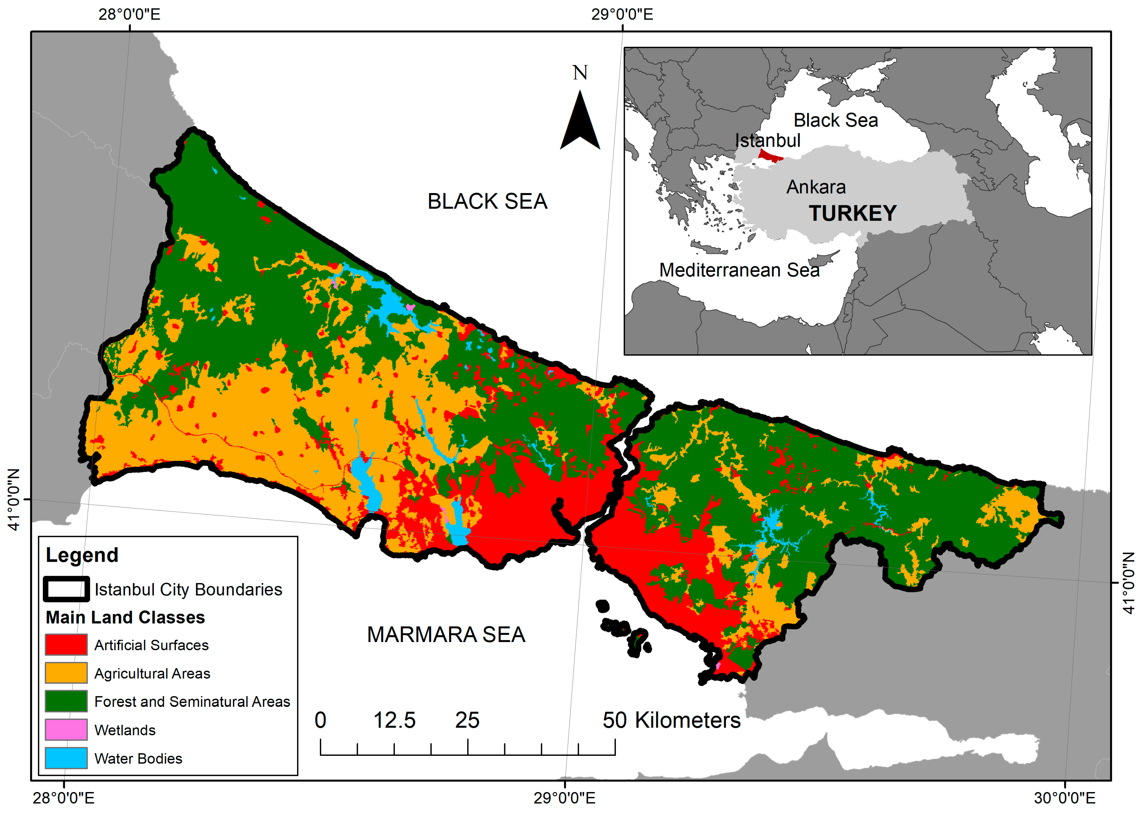
2.1. Study Area
2.2. SWAT Model
2.3. Model Inputs and Setup
3. Results and Discussion
3.1. Calibration and Validation of River Discharges
3.2. Water Availability
4. Conclusions
Acknowledgments
Author Contributions
Conflicts of Interest
References
- IPCC. Climate Change 2013: The Physical Science Basis. Contribution of Working Group I to the Fifth Assessment Report of the Intergovernmental Panel on Climate Change; Stocker, T.F., Qin, D., Plattner, G.-K., Tignor, M., Allen, S.K., Boschung, J., Nauels, A., Xia, Y., Bex, V., Midgley, P.M., Eds.; Cambridge University Press: Cambridge, UK; New York, NY, USA, 2013. [Google Scholar]
- Christensen, J.H.; Kumar, K.K.; Aldria, E.; An, S.-I.; Cavalcanti, I.F.A.; De Castro, M.; Dong, W.; Goswami, P.; Hall, A.; Kanyanga, J.K.; et al. Climate Phenomena and their Relevance for Future Regional Climate Change Supplementary Material. In Climate Change 2013: The physical Science Basis. Contribution of Working Group I to the Fifth Assessment of the Intergovernmental Panel on Climate Change; Cambridge University Press: Cambridge, UK, 2013; pp. 1217–1308. [Google Scholar] [CrossRef]
- Erol, A.; Randhir, T.O. Climatic change impacts on the ecohydrology of Mediterranean watersheds. Clim. Chang. 2012, 114, 319–341. [Google Scholar] [CrossRef]
- World Water Assessment Programme. The United Nations World Water Development Report 3: Water in a Changing World; UNESCO: Paris, France; Earthscan: London, UK, 2009. [Google Scholar]
- Mariotti, A.; Zeng, N.; Yoon, J.-H.; Artale, V.; Navarra, A.; Alpert, P.; Li, L.Z.X. Mediterranean water cycle changes: Transition to drier 21st century conditions in observations and CMIP3 simulations. Environ. Res. Lett. 2008, 3, 44001. [Google Scholar] [CrossRef]
- Biswas, A.K. Water Management for Major Urban Centres. Int. J. Water Resour. Dev. 2006, 22, 183–197. [Google Scholar] [CrossRef]
- Varis, O.; Biswas, A.K.; Tortajada, C.; Lundqvist, J. Megacities and Water Management. Int. J. Water Resour. Dev. 2006, 22, 377–394. [Google Scholar] [CrossRef]
- Falkenmark, M.; Rockström, J. The New Blue and Green Water Paradigm: Breaking New Ground for Water Resources Planning and Management. J. Water Resour. Plan. Manag. 2006, 132, 129–132. [Google Scholar] [CrossRef]
- Schuol, J.; Abbaspour, K.C.; Yang, H.; Srinivasan, R.; Zehnder, A.J.B. Modeling blue and green water availability in Africa. Water Resour. Res. 2008, 44. [Google Scholar] [CrossRef]
- Veettil, A.V.; Mishra, A.K. Water security assessment using blue and green water footprint concepts. J. Hydrol. 2016, 542, 589–602. [Google Scholar] [CrossRef]
- Abbaspour, K.C.; Rouholahnejad, E.; Vaghefi, S.; Srinivasan, R.; Yang, H.; Kløve, B. A continental-scale hydrology and water quality model for Europe: Calibration and uncertainty of a high-resolution large-scale SWAT model. J. Hydrol. 2015, 524, 733–752. [Google Scholar] [CrossRef]
- Rouholahnejad, E.; Abbaspour, K.C.; Srinivasan, R.; Bacu, V.; Lehmann, A. Water resources of the Black Sea Basin at high spatial and temporal resolution. Water Resour. Res. 2014, 50, 5866–5885. [Google Scholar] [CrossRef]
- Rodrigues, D.B.B.; Gupta, H.V.; Mendiondo, E.M. A blue/green water-based accounting framework for assessment of water security. Water Resour. Res. 2014, 50, 7187–7205. [Google Scholar] [CrossRef]
- Zang, C.F.; Liu, J.; Van Der Velde, M.; Kraxner, F. Assessment of spatial and temporal patterns of green and blue water flows under natural conditions in inland river basins in Northwest China. Hydrol. Earth Syst. Sci. 2012, 16, 2859–2870. [Google Scholar] [CrossRef]
- Faramarzi, M.; Abbaspour, K.C.; Schulin, R.; Yang, H. Modelling blue and green water resources availability in Iran. Hydrol. Process. 2009, 23, 486–501. [Google Scholar] [CrossRef]
- TUIK Address-Based Population Registration Database System Turkish Statistical Institute Official Website. Available online: http://www.tuik.gov.tr/UstMenu.do?metod=temelist (accessed on 14 January 2016).
- Van Leeuwen, K.; Sjerps, R. Istanbul: The challenges of integrated water resources management in Europa’s megacity. Environ. Dev. Sustain. 2016, 18, 1–17. [Google Scholar] [CrossRef]
- Istanbul Master Plan Consortium (IMC). Istanbul Water Supply, Sewage and Drainage, Wastewater Treatment, and Disposal Master Plan; Istanbul Master Plan Consortium: Istanbul, Turkey, 1999.
- Akkoyunlu, A.; Yuksel, E.; Erturk, F.; Bayhan, H. Managing of watersheds of Istanbul (Turkey). In Proceedings of the Fifth Water Information Summit: Regional Perspectives on Water Information Management Systems, Ft. Lauderdale, FL, USA, 23–25 October 2002. [Google Scholar]
- Eroglu, V.; Sarikaya, H.Z.; Ozturk, I.; Yuksel, E.; Soyer, E. Water management in Istanbul Metropolitan Area. In Proceedings of the Third International Forum, Integrated Water Management: The key to sustainable water resources, Athens, Greek, 21–22 March 2002. [Google Scholar]
- Yuksel, E.; Eroglu, V.; Sarikaya, H.Z.; Koyuncu, I. Current and Future Strategies for Water and Wastewater Management of Istanbul City. Environ. Manag. 2004, 33, 186–195. [Google Scholar] [CrossRef] [PubMed]
- Altinbilek, D. Water Management in Istanbul. Int. J. Water Resour. Dev. 2006, 22, 241–253. [Google Scholar] [CrossRef]
- Saatci, A.M. Solving Water Problems of a Metropolis. J. Water Resour. Prot. 2013, 5, 7–10. [Google Scholar] [CrossRef]
- Ozturk, I.; Altay, D.A. Water and Wastewater Management in Istanbul. In Proceedings of the UNESCO HQ International Conference on Water, Megacities and Global Change, Paris, France, 1–4 December 2015. [Google Scholar]
- Cuceloglu, G.; Erturk, A. Model Supported Hydrological Analysis of Darlik Creek Watershed, Istanbul Turkey. Fresenius Environ. Bull. 2014, 23, 3110–3116. [Google Scholar]
- Akiner, M.E.; Akkoyunlu, A. Modeling and forecasting river flow rate from the Melen Watershed, Turkey. J. Hydrol. 2012, 456–457, 121–129. [Google Scholar] [CrossRef]
- Kara, F.; Yucel, I. Climate change effects on extreme flows of water supply area in Istanbul: Utility of regional climate models and downscaling method. Environ. Monit. Assess. 2015, 187. [Google Scholar] [CrossRef] [PubMed]
- Istanbul Water and Sewerage Administrationon (ISKI). Climate Change Impacts on Istanbul and Turkey Water Resources Project Final Report; Istanbul Water and Sewerage Administrationon (ISKI): Istanbul, Turkey, 2010.
- Cuceloglu, G.; Ozturk, I. Development of a Model Framework for Sustainable Water Management Practices: Case Study for the Megacity Istanbul. In Proceedings of the 9th Eastern European Young Water Professionals Conference, The International Water Association, Budapest, Hungary, 24–24 May 2017. [Google Scholar]
- Cuceloglu, G.; Ozturk, I. Assessing the Influence of Climate Datasets for Quantification of Water Balance Components in Black Sea Catchment: Case Study for Melen Watershed in Turkey. In Proceedings of the International SWAT Conference, Warsaw, Poland, 26–30 July 2017. [Google Scholar]
- Ezber, Y.; Sen, O.L.; Kindap, T.; Karaca, M. Climatic effects of urbanization in Istanbul: A statistical and modeling analysis. Int. J. Climatol. 2007, 27, 667–679. [Google Scholar] [CrossRef]
- MGM Turkish State of Meteorological Service. Available online: https://www.mgm.gov.tr/veridegerlendirme/il-ve-ilceler-istatistik.aspx?k=undefined&m=ISTANBUL (accessed on 12 January 2017).
- Ozturk, I.; Erturk, A.; Ekdal, A.; Gurel, M.; Cokgor, E.; Insel, G.; Pehlivanoglu-Mantas, E.; Ozabali, A.; Tanik, A. Integrated watershed management efforts: Case study from Melen Watershed experiencing interbasin water transfer. Water Sci. Technol. Water Supply 2013, 13, 1272–1280. [Google Scholar] [CrossRef]
- Arnold, J.G.; Srinivasan, R.; Muttiah, R.S.; Williams, J.R. Large Area Hydrologic Modeling and Assessment Part I: Model Development. J. Am. Water Resour. Assoc. 1998, 34, 73–89. [Google Scholar] [CrossRef]
- Douglas-Mankin, K.R.; Srinivasan, R.; Arnold, J.G. Soil and Water Assessment Tool (SWAT) Model: Current Developments and Applications. Trans. ASABE 2010, 53, 1423–1431. [Google Scholar] [CrossRef]
- Arnold, J.G.; Moriasi, D.N.; Gassman, P.W.; Abbaspour, K.C.; White, M.J.; Srinivasan, R.; Santhi, C.; Harmel, R.D.; Van Griensven, A.; VanLiew, M.W.; et al. SWAT: Model Use, Calibration, and Validation. Asabe 2012, 55, 1491–1508. [Google Scholar] [CrossRef]
- Neitsch, S.L.; Arnold, J.G.; Kiniry, J.R.; Williams, J.R. Soil and Water Assessment Tool Theoretical Documentation Version 2009; Texas Water Resources Institute Technical Report No. 406; Texas A&M University System: College Station, TX, USA, 2011. [Google Scholar]
- Gassman, P.P.W.; Reyes, M.M.R.; Green, C.C.H.; Arnold, J.J.G. The Soil and Water Assessment Tool: Historical development, applications, and future research directions. Trans. ASAE 2007, 50, 1211–1250. [Google Scholar] [CrossRef]
- Food and Agricultural Organization (FAO). The Digital Soil Map of the World and Derived Soil Properties; CD-ROM, Version 3.5; Food and Agriculture Organization of the United Nations, Land and Water Development Division: Rome, Italy, 2003. [Google Scholar]
- Hargreaves, G.L.; Hargreaves, G.H.; Riley, J.P. Agricultural Benefits for Senegal River Basin. J. Irrig. Drain. Eng. 1985, 111, 113–124. [Google Scholar] [CrossRef]
- Ritchie, J.T. Model for predicting evaporation from a row crop with incomplete cover. Water Resour. Res. 1972, 8, 1204–1213. [Google Scholar] [CrossRef]
- USDA. Soil Conservation Service SCS National Engineering Handbook. Section 4, Hydrology. In National Engineering Handbook; USDA: Washington, DC, USA, 1972. [Google Scholar]
- Abbaspour, K.C.; Johnson, C.A.; van Genuchten, M.T. Estimating Uncertain Flow and Transport Parameters Using a Sequential Uncertainty Fitting Procedure. Vadose Zone J. 2004, 3, 1340–1352. [Google Scholar] [CrossRef]
- Abbaspour, K.C.; Yang, J.; Maximov, I.; Siber, R.; Bogner, K.; Mieleitner, J.; Zobrist, J.; Srinivasan, R. Modelling hydrology and water quality in the pre-alpine/alpine Thur watershed using SWAT. J. Hydrol. 2007, 333, 413–430. [Google Scholar] [CrossRef]
- Nash, J.E.; Sutcliffe, J.V. River flow forecasting through conceptual models Part I—A discussion of principles. J. Hydrol. 1970, 10, 282–290. [Google Scholar] [CrossRef]
- Gupta, H.V.; Sorooshian, S.; Yapo, P.O. Status of Automatic Calibration for Hydrologic Models: Comparison with Multilevel Expert Calibration. J. Hydrol. Eng. 1999, 4, 135–143. [Google Scholar] [CrossRef]
- Rouholahnejad, E.; Abbaspour, K.C.; Vejdani, M.; Srinivasan, R.; Schulin, R.; Lehmann, A. A parallelization framework for calibration of hydrological models. Environ. Model. Softw. 2012, 31, 28–36. [Google Scholar] [CrossRef]
- Kamali, B.; Abbaspour, C.K.; Yang, H. Assessing the Uncertainty of Multiple Input Datasets in the Prediction of Water Resource Components. Water 2017, 9. [Google Scholar] [CrossRef]
- Aronica, G.T.; Candela, A. Derivation of flood frequency curves in poorly gauged Mediterranean catchments using a simple stochastic hydrological rainfall-runoff model. J. Hydrol. 2007, 347, 132–142. [Google Scholar] [CrossRef]
- Morlando, F.; Cimorelli, L.; Cozzolino, L.; Mancini, G.; Pianese, D.; Garofalo, F. Shot noise modeling of daily streamflows: A hybrid spectral- and time-domain calibration approach. Water Resour. Res. 2016, 52, 4730–4744. [Google Scholar] [CrossRef]
- Moriasi, D.N.; Arnold, J.G.; Van Liew, M.W.; Bingner, R.L.; Harmel, R.D.; Veith, T.L. Model Evaluation Guidelines for Systematic Quantification of Accuracy in Watershed Simulations. Trans. ASABE 2007, 50, 885–900. [Google Scholar] [CrossRef]
- Covelli, C.; Cozzolino, L.; Cimorelli, L.; Della, M.R.; Pianese, D. A model to simulate leakage through joints in water distribution systems. Water Sci. Technol. Water Supply 2015, 15, 852–863. [Google Scholar] [CrossRef]
- Covelli, C.; Cozzolino, L.; Cimorelli, L.; Della Morte, R.; Pianese, D. Optimal Location and Setting of PRVs in WDS for Leakage Minimization. Water Resour. Manag. 2016, 30, 1803–1817. [Google Scholar] [CrossRef]
- Covelli, C.; Cimorelli, L.; Cozzolino, L.; Della, M.R.; Pianese, D. Reduction in water losses in water distribution systems using pressure reduction valves. Water Sci. Technol. Water Supply 2016, 16, 1033–1045. [Google Scholar] [CrossRef]


| Water Resources | Population | Annual Water Potential (Million m3/Year) |
|---|---|---|
| Asian side * | 5,250,000 | 1909 (77%) |
| European side | 9,750,000 | 568 (23%) |
| Grand annual total | 15,000,000 | 2477 |
| Data Type | Source | Data Resolution |
|---|---|---|
| Digital elevation map (DEM) | Shuttle Radar Topography Mission (SRTM) http://srtm.csi.cgiar.org/ | 90 m |
| Land use | European Environment Agency CORINE Land Cover (year 2000) http://www.eea.europa.eu/data-and-maps/data/corine-land-cover-2000-raster-3 | 100 m |
| Soil | FAO-UNESCO global soil map http://www.fao.org/nr/land/soils/digital-soil-map-of-the-world/en/ | 5 km |
| Climate data | Climate Research Unit http://www.cru.uea.ac.uk | 0.5° |
| Climate Forecast System Reanalysis (CFSR) http://cfs.ncep.noaa.gov/cfsr/ | 0.25° | |
| Turkish State of Meteorological Service http://www.mgm.gov.tr/ | 17 Stations | |
| River discharge | Turkish State of Hydraulics http://en.dsi.gov.tr/ | 25 Stations Monthly |
| Population and water consumption rates | Turkish Statistical Institute http://www.turkstat.gov.tr/Start.do | Yearly |
| Istanbul Water and Sewage Administration www.iski.gov.tr/ |
| SWAT Parameter | Definition | Initial Range | Final Range | t Value | p Value |
|---|---|---|---|---|---|
| r__CN2.mgt | SCS runoff curve number for moisture condition II | −0.5 to 0.5 | −0.20 to 0.39 | −9.742 | 6.73 × 10⁻²¹ |
| r__SOL_AWC().sol | Soil available water storage capacity (mm H2O/mm soil) | −0.5 to 0.5 | −0.06 to 0.80 | 0.390 | 0.696 |
| r__ESCO.hru | Soil evaporation compensation factor | −0.2 to 0.2 | −0.21 to 0.06 | −0.572 | 0.567 |
| r__GW_REVAP.gw | Groundwater revap. coefficient | −0.5 to 0.5 | −0.13 to 0.60 | 0.033 | 0.973 |
| r__GWQMN.gw | Threshold depth of water in shallow aquifer for return flow (mm) | −0.5 to 0.5 | −0.52 to 0.15 | −1.615 | 0.106 |
| r__REVAPMN.gw | Threshold depth of water in the shallow aquifer for ‘‘revap’’ (mm) | −0.5 to 0.5 | −0.50 to 0.16 | 1.695 | 0.090 |
| r__ALPHA_BF.gw | Base flow alpha factor (days) | −0.5 to 0.5 | 0.00 to 0.97 | 4.497 | 8.28 × 10⁻⁶ |
| r__SOL_K().sol | Soil conductivity (mm h−1) | −0.5 to 0.5 | −0.09 to 0.72 | 1.851 | 0.064 |
| r__SOL_BD().sol | Soil bulk density (g cm−3) | −0.5 to 0.5 | −0.03 to 0.89 | 0.011 | 0.990 |
| Gauge Station No. | Calibration | Validation | ||||||||
|---|---|---|---|---|---|---|---|---|---|---|
| P Factor | R Factor | R2 | NSE | PBIAS | P Factor | R Factor | R2 | NSE | PBIAS | |
| 5 | 0.71 | 1.24 | 0.39 | 0.31 | −26.8 | 0.67 | 0.80 | 0.53 | 0.50 | 8.3 |
| 50 | 0.75 | 1.04 | 0.66 | 0.65 | 1.4 | 0.75 | 1.14 | 0.41 | 0.35 | 6.2 |
| 108 | 0.90 | 1.32 | 0.78 | 0.73 | 14.2 | 0.72 | 1.20 | 0.50 | 0.33 | 21.9 |
| 171 | 0.83 | 1.03 | 0.86 | 0.84 | −1.2 | 0.78 | 1.37 | 0.58 | 0.43 | −5.5 |
| 243 | 0.82 | 1.53 | 0.61 | 0.48 | −23.1 | 0.81 | 1.10 | 0.78 | 0.78 | 1.8 |
| 252 | 0.62 | 0.83 | 0.82 | 0.81 | 3.8 | 0.49 | 0.86 | 0.68 | 0.67 | 4.4 |
| 293 | 0.62 | 0.72 | 0.80 | 0.79 | 15.8 | 0.51 | 1.06 | 0.57 | 0.46 | −25.0 |
| 341 | 0.74 | 1.49 | 0.78 | 0.69 | −5.2 | 0.81 | 1.21 | 0.69 | 0.68 | 9.3 |
| 526 | 0.69 | 1.10 | 0.67 | 0.64 | −6.8 | 0.60 | 1.08 | 0.65 | 0.64 | −5.5 |
| 541 | 0.80 | 1.00 | 0.52 | 0.50 | 16.6 | 0.81 | 0.93 | 0.80 | 0.79 | 9.2 |
| 542 | 0.77 | 1.03 | 0.55 | 0.53 | 14.2 | 0.83 | 0.98 | 0.77 | 0.77 | 5.1 |
| 571 | 0.69 | 0.97 | 0.68 | 0.68 | −0.1 | 0.70 | 0.89 | 0.72 | 0.72 | −7.2 |
| 577 | 0.72 | 0.97 | 0.79 | 0.77 | −8.3 | 0.54 | 0.77 | 0.48 | 0.48 | 8.9 |
| 656 | 0.64 | 1.46 | 0.78 | 0.37 | −56.6 | 0.57 | 1.32 | 0.81 | 0.55 | −64.5 |
| 670 | 0.83 | 1.28 | 0.79 | 0.68 | −12.3 | 0.67 | 1.63 | 0.80 | 0.41 | −49.9 |
| 672 | 0.84 | 1.10 | 0.81 | 0.77 | 15.6 | 0.89 | 1.10 | 0.85 | 0.81 | 15.6 |
| 764 | 0.74 | 1.01 | 0.55 | 0.53 | 8.1 | 0.73 | 1.00 | 0.69 | 0.67 | 7.1 |
| 768 | 0.82 | 1.05 | 0.74 | 0.74 | 2.5 | 0.70 | 1.57 | 0.64 | 0.31 | −39.1 |
| 835 | 0.77 | 1.23 | 0.68 | 0.61 | −4.2 | 0.84 | 1.15 | 0.82 | 0.81 | 4.4 |
| 1016 | 0.72 | 1.37 | 0.69 | 0.50 | −33.9 | 0.65 | 1.17 | 0.79 | 0.78 | −13.1 |
| 1028 | 0.73 | 0.70 | 0.64 | 0.59 | 18.3 | 0.74 | 0.89 | 0.69 | 0.61 | 25.3 |
| 1047 | 0.65 | 0.75 | 0.66 | 0.53 | 32.1 | 0.69 | 0.78 | 0.74 | 0.65 | 28.9 |
| 1190 | 0.43 | 0.71 | 0.68 | 0.60 | 3.5 | 0.31 | 1.21 | 0.71 | 0.65 | −31.3 |
| 1230 | 0.78 | 1.20 | 0.74 | 0.72 | −10.3 | 0.76 | 1.18 | 0.74 | 0.74 | −2.0 |
| 1322 | 0.32 | 0.68 | 0.62 | 0.59 | −14.0 | 0.25 | 0.57 | 0.57 | 0.52 | −6.2 |
© 2017 by the authors. Licensee MDPI, Basel, Switzerland. This article is an open access article distributed under the terms and conditions of the Creative Commons Attribution (CC BY) license (http://creativecommons.org/licenses/by/4.0/).
Share and Cite
Cuceloglu, G.; Abbaspour, K.C.; Ozturk, I. Assessing the Water-Resources Potential of Istanbul by Using a Soil and Water Assessment Tool (SWAT) Hydrological Model. Water 2017, 9, 814. https://doi.org/10.3390/w9100814
Cuceloglu G, Abbaspour KC, Ozturk I. Assessing the Water-Resources Potential of Istanbul by Using a Soil and Water Assessment Tool (SWAT) Hydrological Model. Water. 2017; 9(10):814. https://doi.org/10.3390/w9100814
Chicago/Turabian StyleCuceloglu, Gokhan, Karim C. Abbaspour, and Izzet Ozturk. 2017. "Assessing the Water-Resources Potential of Istanbul by Using a Soil and Water Assessment Tool (SWAT) Hydrological Model" Water 9, no. 10: 814. https://doi.org/10.3390/w9100814
APA StyleCuceloglu, G., Abbaspour, K. C., & Ozturk, I. (2017). Assessing the Water-Resources Potential of Istanbul by Using a Soil and Water Assessment Tool (SWAT) Hydrological Model. Water, 9(10), 814. https://doi.org/10.3390/w9100814