Article

Simulating Climate Change Induced Thermal Stress in Coldwater Fish Habitat Using SWAT Model

Department of Geosciences, University of Rhode Island, Kingston, RI 02881, USA
*
Author to whom correspondence should be addressed.
Water 2017, 9(10), 732; https://doi.org/10.3390/w9100732
Submission received: 30 June 2017 / Revised: 31 August 2017 / Accepted: 15 September 2017 / Published: 25 September 2017

Abstract

:
Climate studies have suggested that inland stream temperatures and average streamflows will increase over the next century in New England, thereby putting aquatic species sustained by coldwater habitats at risk. This study uses the Soil and Water Assessment Tool (SWAT) to simulate historical streamflow and stream temperatures within three forested, baseflow-driven watersheds in Rhode Island, USA followed by simulations of future climate scenarios for comparison. Low greenhouse gas emission scenarios are based on the 2007 International Panel on Climate Change Special Report on Emissions Scenarios (SRES) B1 scenario and the high emissions are based on the SRES A1fi scenario. The output data are analyzed to identify daily occurrences where brook trout (Salvelinus fontinalis) are exposed to stressful events, defined herein as any day where Q25 or Q75 flows occur simultaneously with stream temperatures exceeding 21 °C. Results indicate that under both high- and low-emission greenhouse gas scenarios, coldwater fish species such as brook trout will be increasingly exposed to stressful events. The percent chance of stressful event occurrence increased by an average of 6.5% under low-emission scenarios and by 14.2% under high-emission scenarios relative to the historical simulations.

1. Introduction

Concerns have arisen regarding the impact of warming stream temperatures on brook trout (Salvelinus fontinalis) habitat due to climate change. Over the next century, freshwater ecosystems in the New England region of the United States are expected to experience a continued increase in mean daily stream temperatures and an increase in the frequency and magnitude of extreme high flow events due to warmer, wetter winters, earlier spring snowmelt, and drier summers [1,2,3,4,5,6,7,8,9]. As the spatial and temporal variability of stream temperatures play a primary role in distributions, interactions, behavior, and persistence of coldwater fish species [7,10,11,12,13,14,15,16], it has become increasingly important to understand what challenges freshwater fisheries managers will face because of climate change. Analytical models such as the Soil and Water Assessment Tool (SWAT) [17] can be used to estimate the effects of climate change on stream temperatures and aquatic species [5,18,19,20,21,22,23,24]. Several studies have used global climatic model output or temperature and precipitation variations to drive hydrologic and stream temperature models for the United States [25] and worldwide [8]. This study uses both SWAT and global climate data downscaled for New England [3,4,26,27,28] to simulate the effects of increasing air temperatures and changes to regional rainfall patterns on coldwater fish habitats in southern New England watersheds.
The SWAT model was used to generate historical and future stream temperature and streamflow data, followed by an assessment of the frequency of “stressful events” affecting the Rhode Island native brook trout. Brook trout, a coldwater salmonid, is a species indicative of high water quality and is also of interest due to recent habitat and population restoration efforts by local environmental groups and government agencies [29,30]. This fish typically spawns in the fall and lays eggs in redds (nests) deposited in gravel substrate. Eggs develop over the winter months and hatch from late winter to early spring [11,12,31]. The life cycle of brook trout, however, is heavily influenced by the degree and timing of temperature changes. High stream temperatures cause physical stress including slowed metabolism and decreased growth rate, adverse effects on critical life-cycle stages such as spawning or migration triggers, and in extreme cases, mortality [7,10,32,33,34,35]. Distribution is also affected as coldwater fish actively avoid water temperatures that exceed their preferred temperature by 2–5 °C [36,37]. Studies have shown that optimal brook trout water temperatures are below 20 °C, symptoms of physiological stress develop at approximately 21 °C [33] and temperatures above 24 °C have been known to cause mortality in this species [12].
Flow regime is another critical factor in maintaining the continuity of aquatic habitats throughout a stream network [35,38,39,40,41,42,43]. While temperature is often cited as the limiting factor for brook trout, the flow regime has equal importance [44]. Alteration of the flow regime can result in changes in the geomorphology of the stream and the distribution of food-producing areas as riffles and pools shift. Changes in the distribution of riffles and pools can cause a decrease in food-producing areas, reduced macroinvertebrate abundance and more limited access to spawning sites or thermal refugia [12,31,45,46]. Reductions in flow have a negative effect on the physical condition of both adult brook trout and young-of-year. Nuhfer et al. found a significant decline in spring-to-fall growth of brook trout when 75% flow reductions occurred [45]. The consequences of lower body mass are not always immediately apparent. Adults may suffer higher mortality during the winter months following the further depletion of body mass due to the rigors of spawning. Poor fitness of spawning adults may result in lower quality or abundance of eggs and a decline in hatching during the late winter to early spring [31]. Velocity of water through the stream reach can affect sediment and scouring of the stream bed and banks, reducing the availability of nest sites or, in the event of low flows, cause water temperatures to rise.
To address the importance of both stream temperature and flow regime, “stressful events” are defined herein as days where either high or low flow occurs simultaneously with stream temperatures exceeding 21 °C. For the purpose of this study, high and low flows will be considered as the values exceeding the 25-percent and 75-percent percentiles (Q25, Q75) for both historical and future simulated SWAT model output. Two Wood-Pawcatuck River headwater subbasins, the Queen River and the Beaver River, were selected as study sites due to their pristine, undisturbed aquatic habitat. A third pristine watershed, Cork Brook, was chosen as a study site because of its association with the Scituate Reservoir, which supplies drinking water to the city of Providence, Rhode Island. This study incorporated two climate change scenarios for future stream conditions at the three project sites. Low greenhouse gas emission scenarios are based on the 2007 International Panel on Climate Change Special Report on Emissions Scenarios (SRES) B1 scenario and the high-emission scenarios are based on the SRES A1fi scenario. Model output was analyzed over four time periods: historical (1980–2009), short term (2010–2039), medium term (2040–2067) and long term (2070–2099) to understand how coldwater habitat in these watersheds will react to climate change over the next century. Results provide a site-specific approach for watershed managers trying to determine the types and distribution of future habitat risk to coldwater species. As the demands for water quality and quantity increase for wildlife and human consumption over the next century, new evaluation techniques will help anticipate and solve unprecedented challenges. In the Wood-Pawcatuck and Cork Brook watersheds, the anticipated challenges may include an increase in stressful conditions.

2. Materials and Methods

2.1. Study Sites

Three watersheds were selected to achieve the objective: Queen River, Beaver River and Cork Brook. The Queen and Beaver watersheds lie adjacent to each other within the Wood-Pawcatuck watershed in southern Rhode Island (Figure 1). In its entirety, the 800 km2 watershed is comprised of seven drainage basins and two major rivers. The upper reaches of the Wood-Pawcatuck watershed trend towards undisturbed rural environments. The watershed becomes increasingly urban and impaired towards the downstream reaches before emptying into Little Narragansett Bay. This watershed supports native brook trout populations, high-quality wildlife habitat and a species diversity that is unique for a watershed of this scale in southern New England [30,47,48,49,50,51,52,53,54,55,56]. The effect of climate change on stream water quality is a serious concern in Wood-Pawcatuck watershed and many non-profit organizations, recreational fishing groups and government agencies have taken interest in the long-term survival of local brook trout.
The Beaver River and the Queen River watersheds cover areas of approximately 23 and 52 km2, respectively. Many similarities exist between the two subbasins. Land use is primarily forest although wetlands and agriculture make up a small portion of each watershed. Both are HUC 12 river headwaters to the larger Pawcatuck river and each watershed hosts nature preserves owned and managed by The Nature Conservancy [54,57]. Continuous and permanent United States Geological Survey (USGS) gauges have been recording flow data for several decades within each river [58]. The Beaver River USGS gauge (number 01117468) is located near Usquepaug, RI where it intersects State Highway 138, or approximately 5.8 km upstream from its confluence with the Pawcatuck River. The gauge has been in continual operation since 1974. Mean daily discharges at the Beaver River gauge are typically lowest in September (0.02 m3/s) and highest in April (1.04 m3/s), with annual mean daily discharge of 0.59 m3/s. USGS gauge station (number 01117370) is located on the intersection between the Queen River and Liberty Road, and data has been recording since 1998. Discharges at the Queen River gauge are higher, historically lowest in August (0.039 m3/s) and highest in March (2.08 m3/s) with mean daily discharges of approximately 1.06 m3/s. A separate analysis of groundwater contributions to stream discharge was conducted using an automated method for estimating baseflow [59]. A noteworthy difference between the two watersheds is the baseflow contributions to each river, 93% within the Beaver River and 78% for the Queen River.
The third study site is Cork Brook in Scituate, Rhode Island. This small forested watershed is a tributary to the Scituate Reservoir, which is part of the larger Pawtuxet River basin beginning in north-central Rhode Island and eventually flowing into Narragansett Bay. The Scituate Reservoir is the largest open body of water in the state and is the main drinking water source to the city of Providence. Cork Brook is approximately four km long and covers an area of approximately seven km2. Human disturbance within the watershed is minimal and most of the land use within the watershed is undeveloped forest and brushland, although a portion (14%) of land use within the watershed is classified as medium density residential. USGS station number 01115280 is located on Rockland Road near Clayville, RI, which has been continuously recording streamflow at the site since 2008 [58]. A primary difference between the Cork Brook and Wood-Pawcatuck watersheds is size and the stream discharge amounts. The mean daily discharges at the gauge are historically lowest in September (0.025 m3/s), highest in March (0.27 m3/s) and annually average approximately 0.11 m3/s. Average daily stream temperature is estimated at 7.8 °C since 2001. An important similarity to the Beaver and Queen watersheds is groundwater contribution; baseflow contributes the majority (60%) of stream discharges.

2.2. Model Setup

This study uses the hydrologic and water quality model SWAT for simulating streamflow and stream temperature. SWAT is a well-established, physically-based, semi-distributed hydrologic model created by the United States Department of Agriculture (USDA) in 1998 [17,60,61,62]. Surface water runoff and infiltration volumes are estimated using the modified soil conservation service (SCS) 1984 curve number method, and potential evapotranspiration is estimated using the Penman–Monteith method [63,64]. Stream temperature is estimated from air temperature based on a linear regression method developed by Stefan and Prued’homme [17,65]:
T w ( t ) = 5.0 + 0.75 T a i r ( t δ )
where ( T W ) represents average daily water temperature (°C), ( T a i r ) represents and average daily air temperatures (°C). Time (t) and lag (δ) are in days. Water temperatures follow air temperatures closely, the time lag for a shallow stream is expected to be on the order of a few hours due to the thermal inertia of the water [65]. The average relationship indicates that when the daily air temperature is close to 0 °C then the water will be approximately 5 °C warmer. When the daily air temperature is below 20 °C the water temperature is likely to be greater than the air temperature [65]. The Rhode Island Geographic Information System (RIGIS) database is the main source for the spatial data used as model inputs [66]. RIGIS is a public database managed by both the RI government and private organizations. Typical SWAT model inputs in ArcSWAT [67] include topography, soil characteristics, land cover or land use and meteorological data. Information collected for this study includes the following: 2011 Land use/land cover data derived from statewide 10-m resolution National Land Cover Data imagery [68]; soil characteristics collected from a geo-referenced digital soil map from Natural Resource Conservation Service (NRCS) Soil Survey Geographic database (SSURGO) [69]; and topography information extracted from USGS 7.5-min digital elevation models (DEMs) with a 10-m resolution. Regional meteorological data from 1979 to 2014 including long term precipitation and temperature statistics were downloaded from Texas A&M University’s global weather data site [70,71].
Based on the spatial data provided, SWAT delineated the watersheds into HRU units, which are represented as a percentage of the subbasin area. The user sets a soil, land and slope threshold based on the level of heterogeneity within a watershed and when a parcel of land meets or exceed all thresholds a HRU is created. The Beaver River basin is generally homogenous and was delineated into five subbasins and 12 HRUs using land, soil and slope thresholds of 20%. The Queen River has more variability in the type and distribution of land use throughout the watershed. This watershed was delineated into eight subbasins and 17 HRUs using land, soil and slope thresholds of 25%, 20% and 20%. Cork Brook was delineated in SWAT to create four subbasins and 27 HRUs using land, soil and slope thresholds of 20%, 10% and 5%. The soil types and elevation changes are variable throughout the Cork Brook watershed and as such these thresholds were reduced to capture basin heterogeneity.

2.3. Model Calibration & Validation

The SWAT Calibration and Uncertainty Program (SWAT-CUP), Sequential Uncertainty Fitting Version 2 (SUFI-2) [72,73], was used to conduct sensitivity analysis, calibration and model validation on daily stream discharge from the output hydrograph. Performance was measured using coefficient of determination and Nash-Sutcliffe Efficiency (NSE) and percent bias (PBIAS). Coefficient of determination (R2) identifies the degree of collinearity between simulated and measured data and NSE was used as an indicator of acceptable model performance. R2 values range from 0 to 1 with a larger R2 value indicating less error variance. NSE is a normalized statistic that determines the relative magnitude of the residual variance compared to the measured data variance [74]. NSE ranges from −∞ to 1; a value at or above 0.50 generally indicates satisfactory model performance [60,75,76,77]. This evaluation statistic is a commonly used objective function for reflecting the overall fit of a hydrograph. Percent bias is the relative percentage difference between the averaged modeled and measured data time series over (n) time steps with the objective being to minimize the value [78]. The model was validated by using calibrated parameters and performance checked using NSE, R2 and percent bias.
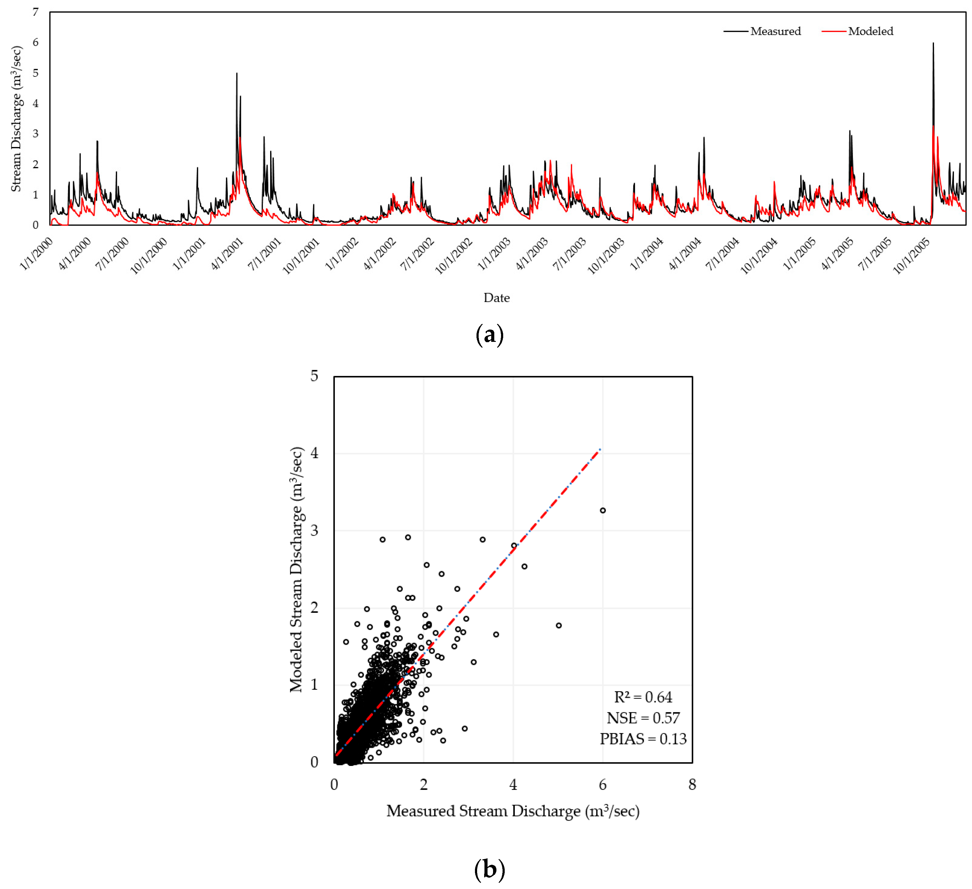
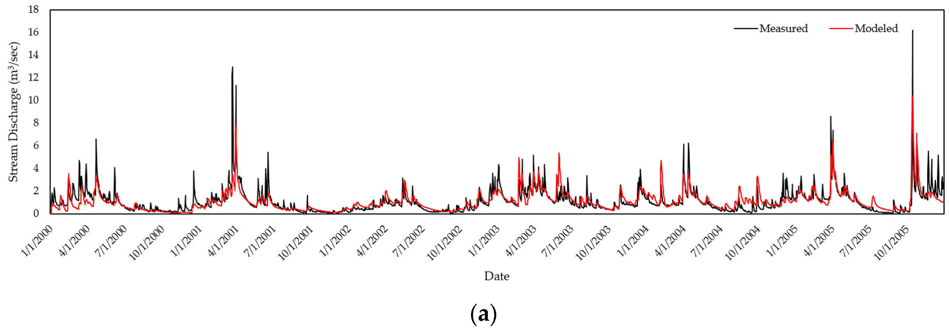
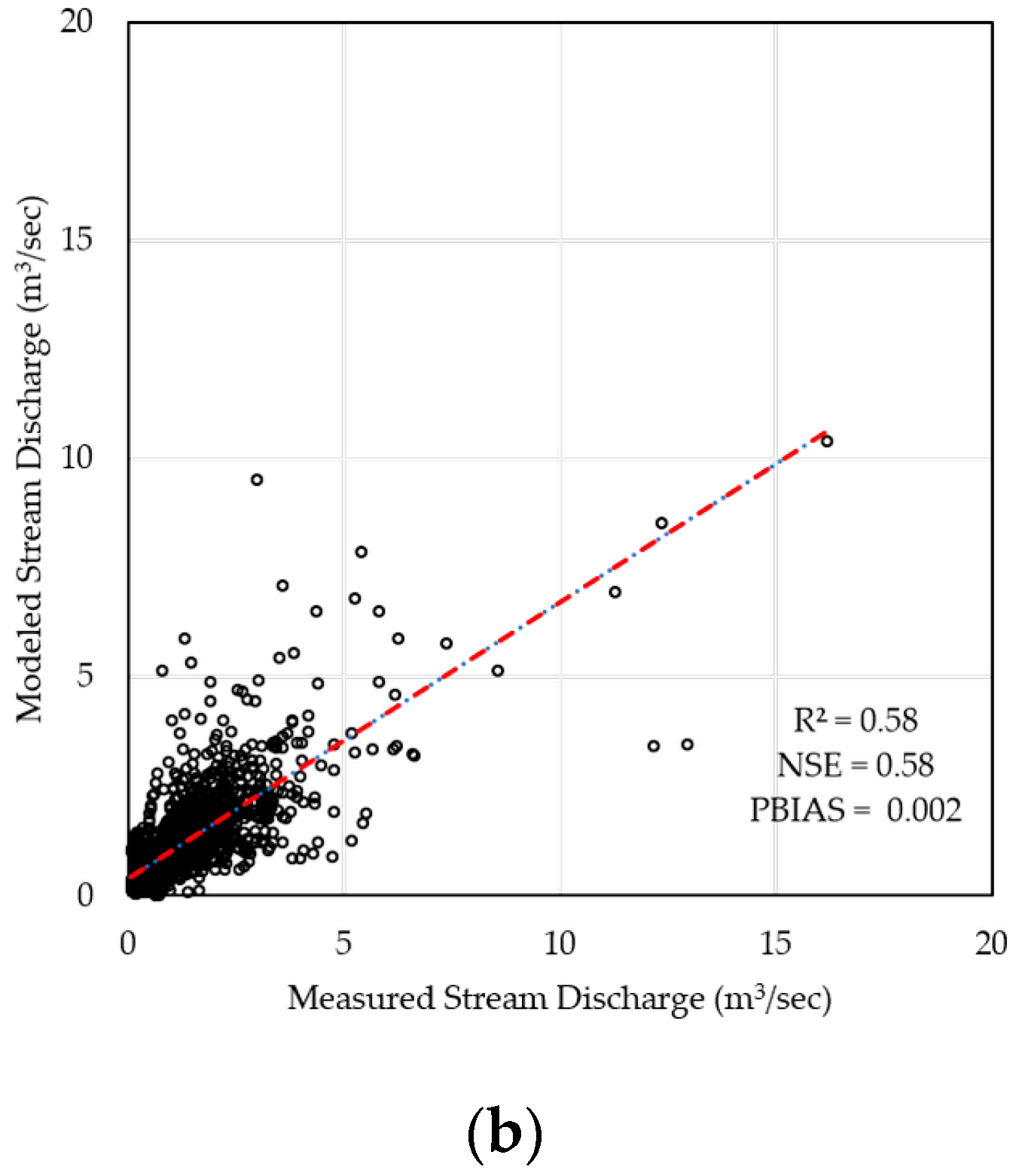
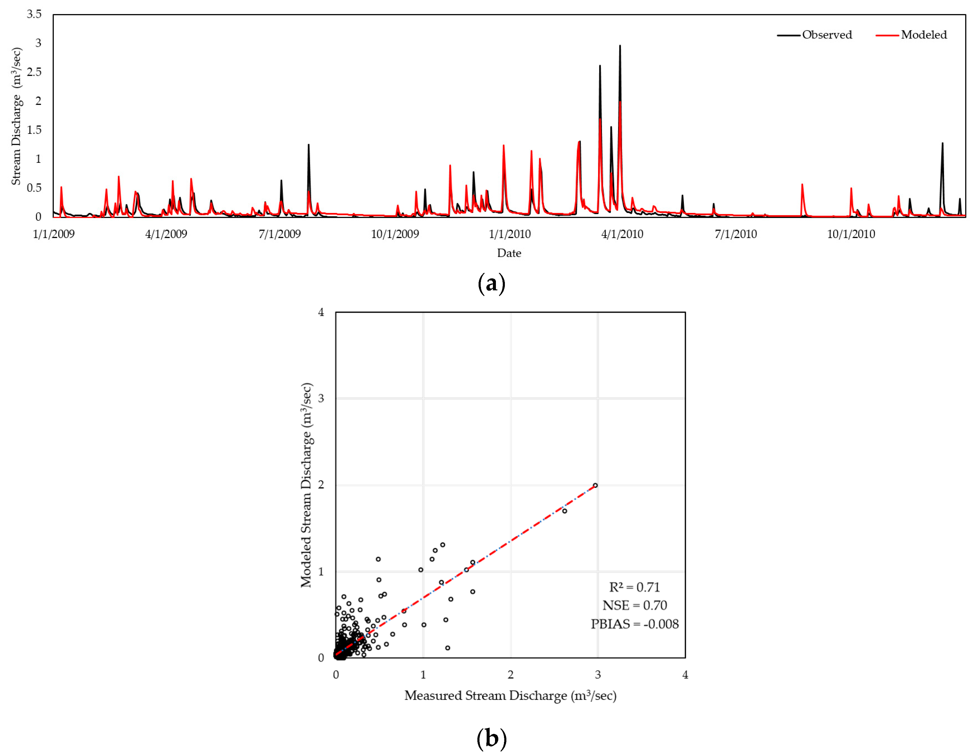
Each model was run for the entire period of precipitation and rainfall data availability (1979–2014) and then calibrated for daily streamflow in SWAT-CUP via SUFI-2 using a portion of the existing observed data at each associated USGS gauge. The Beaver River and Queen River watersheds were calibrated over the same five-year time span from 2000 to 2005 due to data availability and avoidance of natural streamflow anomalies in 2010 and 2006. Validation occurred from 2007 to 2008 in both the Beaver and Queen River watersheds. Meanwhile, the Cork Brook model was calibrated for streamflow over a shorter two-year time-span from 2009 to 2010 due to a limited availability in observed discharge data (2008–present). The Cork Brook model was validated for the year 2012 because the 2011 data showed evidence of discharge anomalies and 2013 weather data were incomplete. The modeled hydrographs versus the observed hydrographs are shown in Figure 2, Figure 3 and Figure 4 and the statistical results of calibration and validation are shown in Table 1 and Table 2.
The most sensitive parameters in daily streamflow calibration are summarized in Table 3 and were primarily related to groundwater and soil characteristics. The alpha-BF (baseflow) recession value was one of the most effective parameters for all three models and the values were all very small. The alpha baseflow factor is a recession coefficient derived from the properties of the aquifer contributing to baseflow; large alpha factors signify steep recession indicative of rapid drainage and minimal storage whereas low alpha values suggest a slow response to drainage [59,79]. Alpha-bnk (bankflow) was another sensitive parameter, which is simulated with a recession curve like that used for groundwater. For this parameter, a high value at all three sites indicates a flat recession curve, which is similar to the alpha-bf value that specifies a slow response to drainage. The threshold depth of groundwater in the shallow aquifer (GWQMN) is small and very similar between all three models, less than a meter within each. This is the threshold water level in the shallow aquifer for groundwater contribution to the main channel to occur. Since groundwater accounts for the majority of stream discharge at all sites the sensitivity of soil and groundwater parameters was expected.

2.4. Climate Change Variables

The anticipated change in average air temperature and precipitation over short term (2010–2039), medium term (2040–2069) and long term (2070–2099) time-spans for low and high greenhouse gas (GHG) scenarios were incorporated and compared to the historical period (1980–2009). Low greenhouse gas emission scenarios are based on the 2007 International Panel on Climate Change SRES B1 scenario and the high emissions are based on the SRES A1fi scenario. The B1 scenario is a situation where economic growth incorporates clean, ecologically friendly technology and GHG emissions levels return to pre-industrial concentrations, estimated at CO2 levels of 300 parts per million (ppm). The high-emission scenario (A1fi) is a scenario based on fossil fuel intensive technologies for worldwide economic growth resulting in CO2 levels reaching 940 ppm.
Climate variables in the calibrated SWAT subbasin input files (.sub) were edited to simulate the future scenarios. The default carbon dioxide (CO2) concentration, relative rainfall adjustment and temperature increases (°C) are 330 parts per million (ppm), zero and zero respectively. The default values within all .sub files for each model were replaced with climate change variables. The variables used in this study are based on values published by Wake et al. at the University of New Hampshire [26,27,28], which were generated from four global climatic models downscaled to the New England region. Two of the published climate grids for Rhode Island were adopted and modified for this study and four different CO2 levels were used. SWAT output for all low-emission scenarios is based on 330 ppm (the lower limit in the SWAT program code) and the RI climate grid change factors in Table 4a,c. For the high-emission alternatives, the short, medium and long-term SWAT climate change simulations were run with CO2 levels at 540, 740 and 940 ppm, respectively, in addition to the RI climate grid change factors in Table 4b,d.

2.5. Stressful Event Identification

Upon model calibration, validation and incorporation of climate change variables, output data for both model versions were processed to predict the occurrence of stressful conditions in all three watersheds from 1980 to 2099. As previously discussed, a stressful event for this study is defined as any day where both temperature and flow extremes occur. This study used the Q25 and Q75 flow exceedance percentiles as indicators because of their common use [80,81,82] and ecohydrological importance to brook trout. The most critical period for the species is typically the lowest flows of late summer to winter and a base flow of <25% is considered poor for maintaining quality trout habitat [12,44]. A Q25 exceedance characterizes the highest 25% of all daily flow rates and Q75 represents the lowest 25% of all daily flow rates [82]. For the stressful event analysis, the exceedance probability and average daily stream temperature for each date were identified. If the day fell into the Q25 or Q75 percentile, and if the stream temperature was greater than 21 °C, then the day was tagged as being a thermally stressful event.

3. Results and Discussion

3.1. Historical Conditions

The modeled average daily stream temperature was nearly the same at all three sites. The average daily discharge, however, was different at all three sites and corresponded to watershed area, with the highest discharge within the Queen River (largest watershed) and the lowest discharge within Cork Brook (smallest watershed) (Table 5). This is in agreement with the observed data, the Queen River had the highest discharge followed by the Beaver River and Cork Brook. The calibrated model for each watershed was first run over the entire 30-year period (1980–2009) (Table 5) to understand the percent chance that a stressful event will occur on a given day. Of the three study sites, the Queen River had the highest percent chance that a stressful event would occur on any given day and the Beaver River had the lowest percent chance (Table 6).
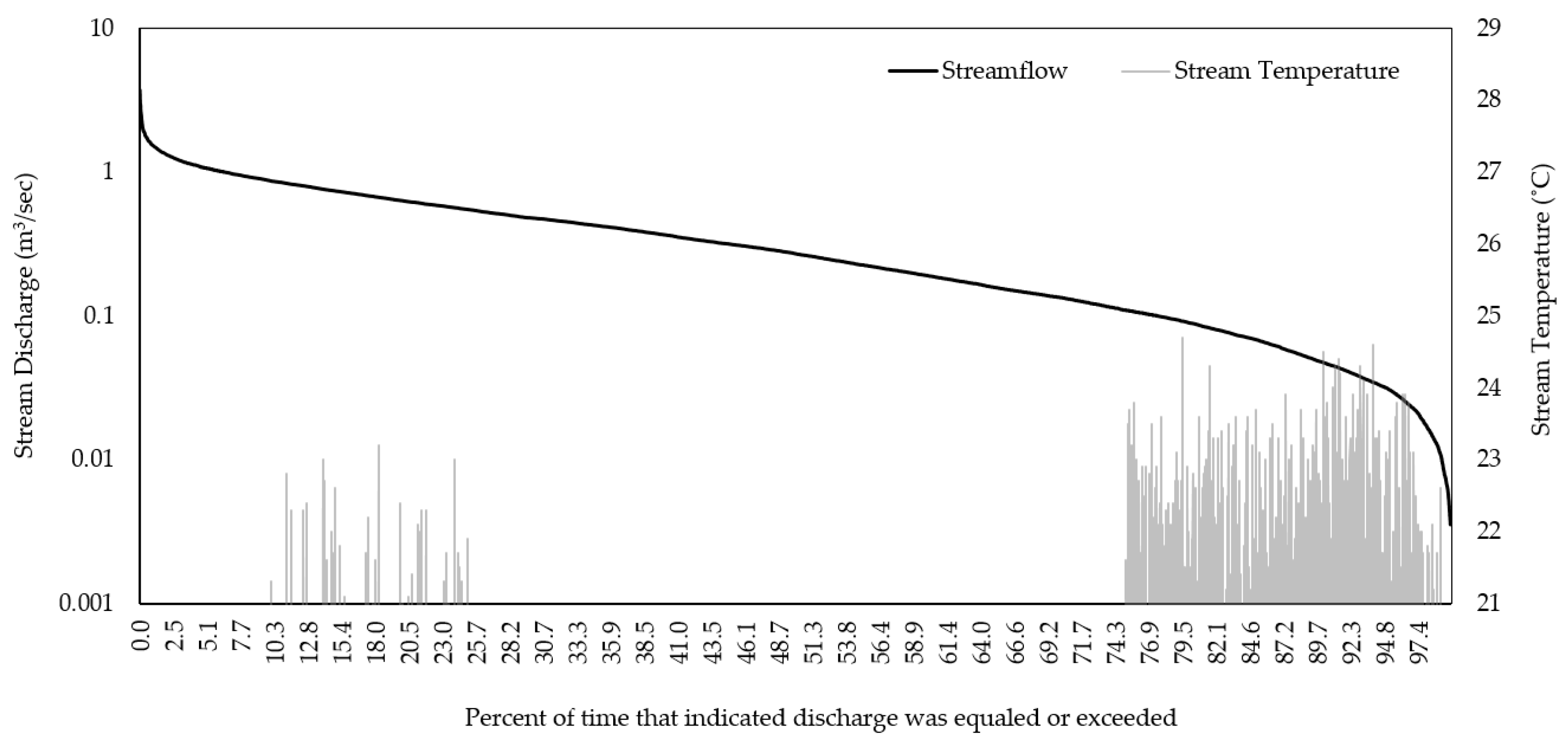
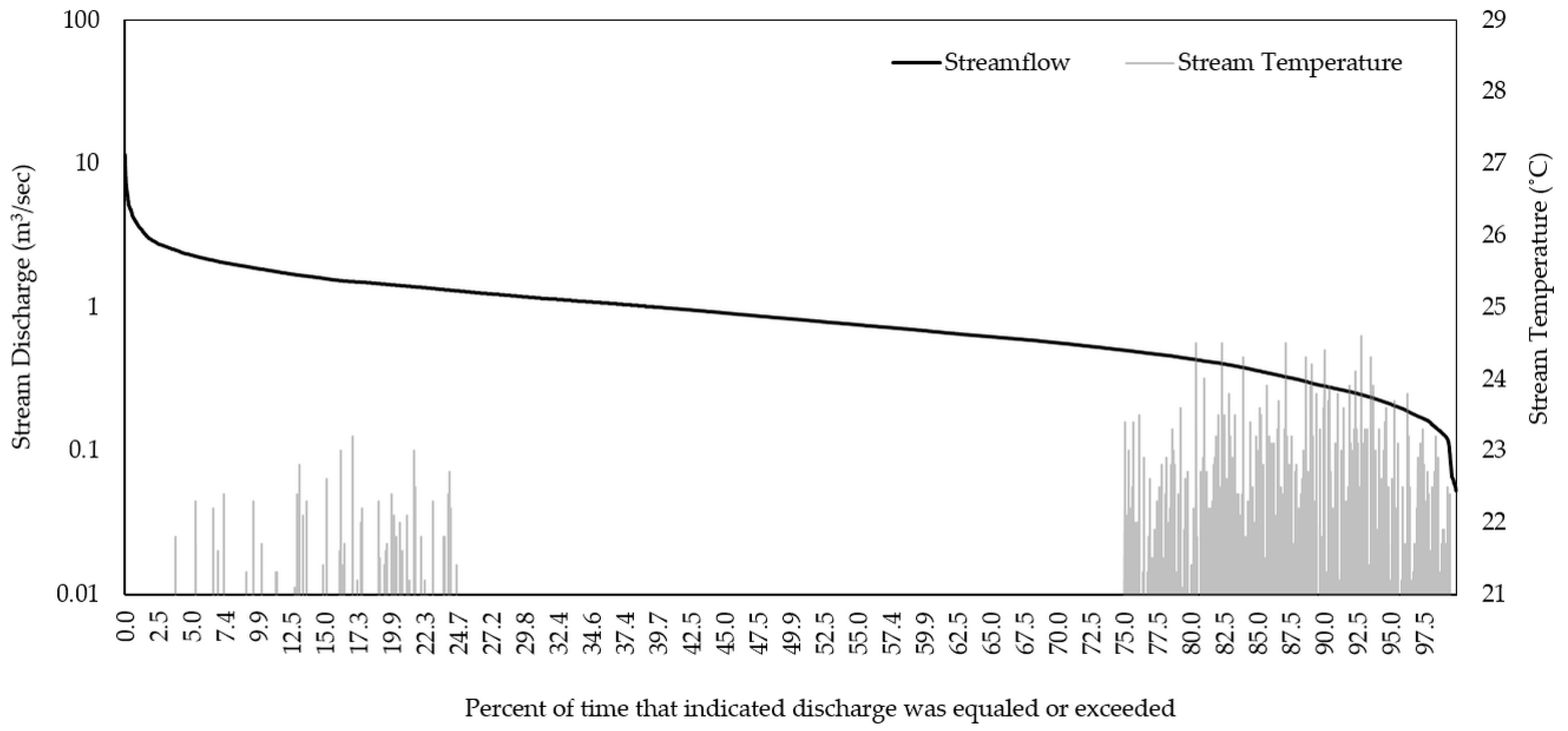
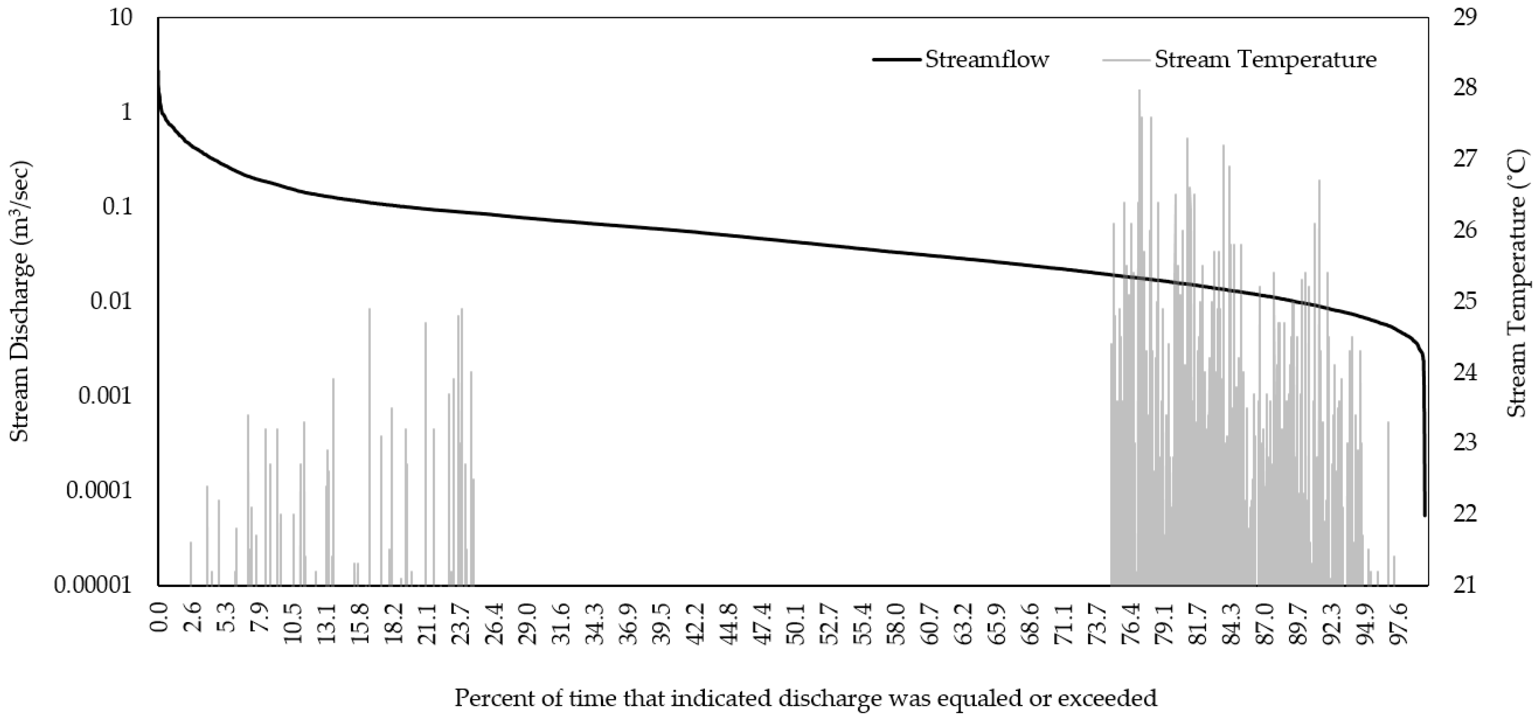
The frequency of stress events in the three watersheds are similar (Table 6). The chances of any type of stress occurring within the watersheds vary by just 1.1%. One difference between Cork Brook and the Pawcatuck watersheds is the number of days with stream temperatures greater than 21 °C. The Beaver River and the Queen River have the same number of days with temperature stress because the air temperature for each model was collected from the same weather station. The number of days with stream temperature greater than 21 °C at Cork Brook is 46% higher than the Pawcatuck watersheds. This may be attributed to the low discharge levels at Cork Brook (0.081 m3/s) because lower, slower flows are exposed to air longer causing them to increase or decrease in temperature more readily. This interpretation is illustrated in Figure 5, Figure 6 and Figure 7, which show the distribution of high stream temperatures within the Q25 and Q75 percentiles for each watershed. For all watersheds, a greater number of stressful events occurred during periods of low flow rather than periods of high flow.
Lastly, it is interesting to note the occurrences of stressful events within each watershed. Even though the Queen River has the same number of temperature stress days as the Beaver River, a difference of only 90 flow stress days increased the percent chance of stressful event occurrences from 4.7% in the Beaver River to 5.5% chance in the Queen River. This shows that a combination of flow and temperature should be taken into consideration when making management decisions or evaluating the quality of aquatic habitat. Such details can have important implications for aquatic species. Brook trout have been observed to tolerate higher stream temperatures provided their physical habitat remains stable [45]. If the co-occurrence of temperature and flow stresses increases, then physiological stresses to individual trout may become more apparent. The data simulated from 1980 to 2009 provide a baseline for comparing future projections, and will help determine if the resilience of local brook trout populations may become strained under future climate change conditions by combining two important indicators for survival.

3.2. Future Projections

New England is predicted to experience a warmer and wetter climate due to global warming [3]. Since 1970, Rhode Island specifically has had the average maximum and minimum air temperatures increase by 1.2 °C annually and by 2020–2099 it is expected that there will be hotter summers with 12–44 more days above 50 °C [26]. Also since 1970, the frequency and magnitude of extreme precipitation events has increased and annual precipitation has increased 6–11%. By 2020–2099, annual precipitation averages will increase by 18–20% and a two-fold increase in extreme precipitation events is expected to occur. A decrease in snow cover is anticipated and Rhode Island may have 20–32 fewer snow covered days [26].

3.2.1. Stream Discharge and Stream Temperature

Within the Beaver and Queen Rivers the simulated stream discharge change was much greater for high CO2 emission scenarios 2010–2099 than for low CO2 emission scenarios, a change of 3.4 °C as opposed to 1.6 °C, respectively. Discharges between the two Wood-Pawcatuck subbasins were different and a greater change was observed in the Beaver River subbasin. In the Beaver River, under the low-emission scenario 2010–2099 the discharges increased by 23% related to historical discharges and under the high-emission scenario increased by 71%. In the Queen River, under the low-emission scenario 2010–2099 the discharges increased by 19% of historical discharge levels and under the high-emission scenario increased by 49%. This is interesting because groundwater inputs are greater in the Beaver River (93%) than in the Queen River (78%). In the New England region, baseflow contributions have shown an upward trend likely linked to increasing precipitation [83] and climate change may be impacting storage by increasing the volume of water held in groundwater or as soil moisture within the basin. When storage is exceeded, the upper streamflow quantiles may be affected [84]. Brook trout can benefit from increased baseflow. Groundwater inflow can cool stream water [85], especially when flows are lower in the summer months [86]. Brook trout rely on groundwater seeps as refugia from increased stream temperatures and to keep developing embryos submerged in cool water [12].
An increase in stream temperature and streamflow was also seen in Cork Brook. Stream temperature increased by 1.6 °C between 2010 and 2099 under the low-emission scenario and 3.5 °C under the high-emission scenario, very similar to the degree changes in the Pawcatuck watersheds. Between 2010 and 2099, discharges increased by 20% under the low-emission scenario and 60% under the high-emission scenario. While not exact, the changes in discharge at Cork Brook for the low-emission scenario are more similar to the changes within the Queen River based on percent increase although under the high-emission scenario Cork Brook is the median between the Beaver River and Queen River. Overall, the SWAT streamflow projections in the three watersheds align well with climate change predictions for New England under the low-emission simulations and exceed predictions under the high-emission simulations [26]. The modeled average daily stream temperature and average daily stream discharge increased at all sites for both low and high CO2 emission scenarios (Table 7).

3.2.2. Flow Regime

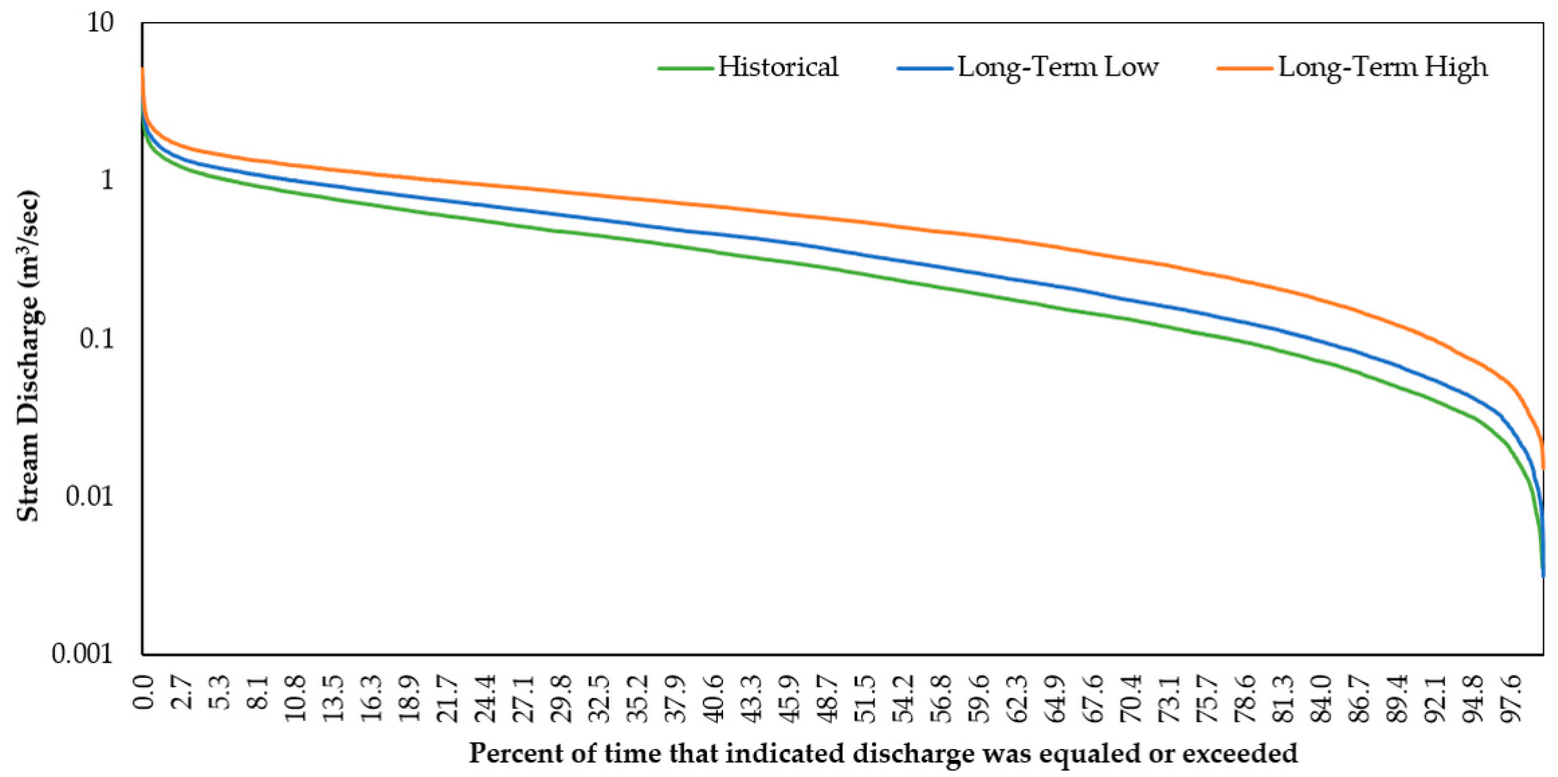
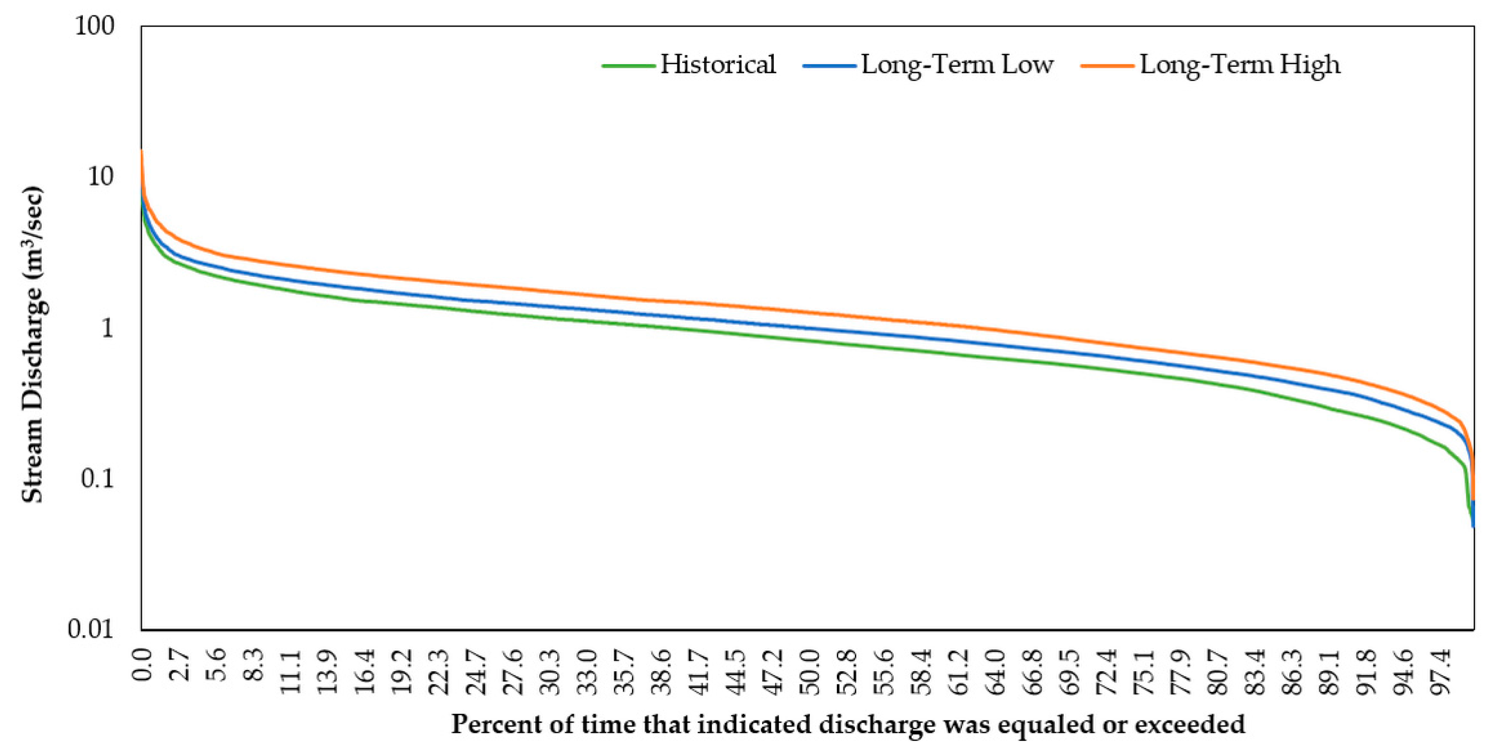
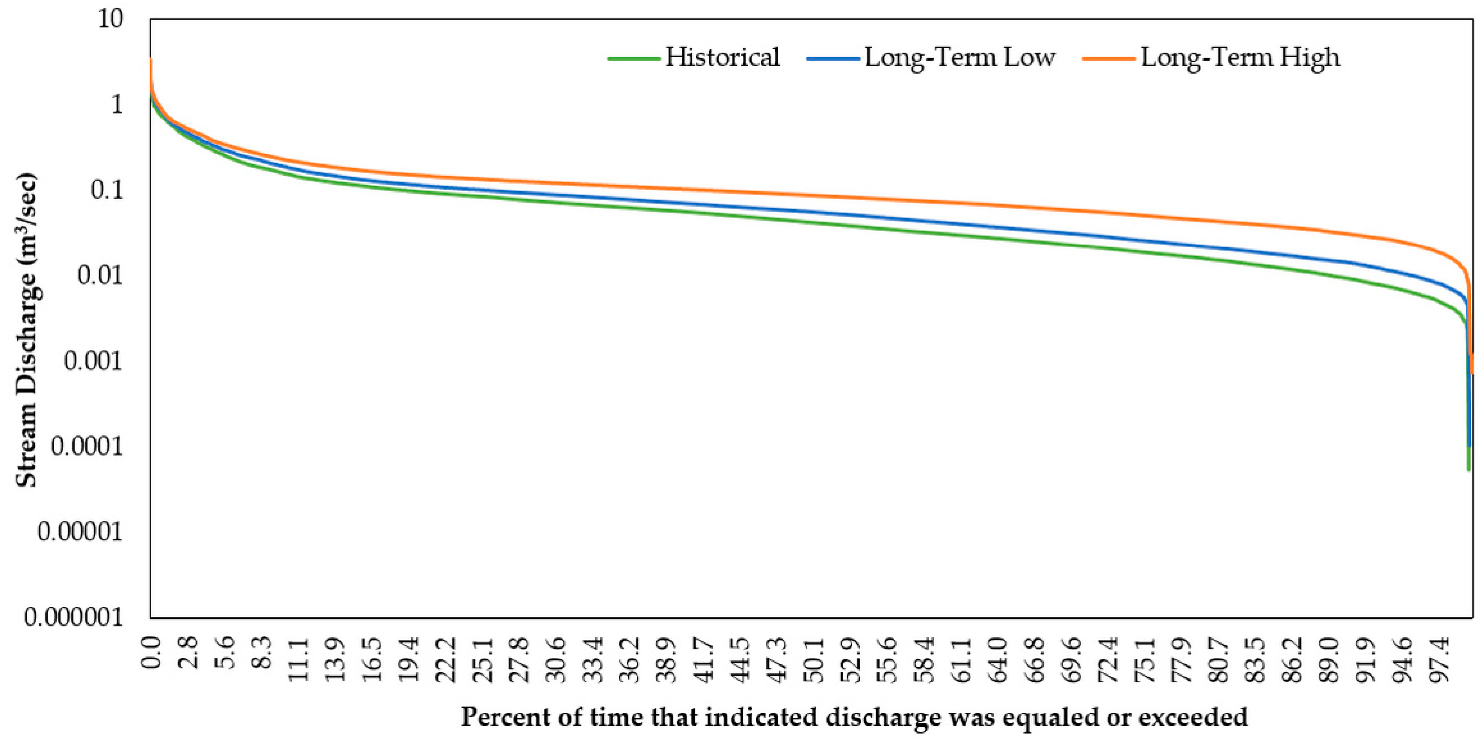
The flow duration curves for each watershed were compared to historical streamflow (1980–2009) and future long term (2070–0299) scenarios to assess the flow conditions at the end of the century (Figure 8, Figure 9 and Figure 10). The curve for each watershed under the low emission scenarios changed very little in shape even though the stream discharges were increased. Under the high-emissions scenario the magnitude of discharges also increases but in the Beaver River and Cork Brook, the shape of the rating curve became flatter in the Q50–Q75 percentiles. A flat curve generally indicates that flows are sustained throughout the year and can be caused by factors such as groundwater contributions to the stream reach.
As water temperatures increase due to global warming, brook trout may benefit from sustained flows that will prevent stream temperatures from rising further and help ensure that downstream habitat remains connected to headwaters. From this perspective, the Beaver River and Cork Brook may provide better future trout habitat in comparison to the Queen River, which saw little change to the shape of the rating curve. On the other hand, a sustained increase in flow magnitude can change the geomorphology and may not be beneficial for aquatic species during the spawning season when flows are historically lower [41]. An increase in stream discharges during the low flow season may put redds (nests) at risk of destruction from sedimentation or sheer velocity. Changes in streamflow magnitude may also increase turbidity or redistribute riffle and pool habitat throughout the stream reach. This may decrease the availability of suitable habitat as brook trout prefer stream reaches with an approximate 1:1 pool-riffle [12]). Pool and riffle redistribution can also affect the type and quantity of local macroinvertebrate populations. Since warming temperatures will have an impact on trout body condition as fish enter the winter months, the available food supply can become an even more critical factor as the climate changes.

3.2.3. Timing of Stream Temperatures

The model predicted that between 1980 and 2099 stream temperatures in all watersheds will increase by 1.6 °C under the low-emission scenario or 3.4 °C under the high-emission scenarios (Table 7). Further analysis was conducted to assess if the temporal distribution of stream temperatures has changed throughout the year. In the Beaver and Queen River watersheds no change to the timing of high stream temperatures was observed and high temperatures continued to occur primarily in July–September (Figure 11a). In the Cork Brook watershed, however, the model predicted that the occurrence of high stream temperatures will increase and will occur as early as April by the end of the century under both high- and low-emission scenarios (Figure 11b). In all watersheds, the number of days with stressful temperatures during the low-emission scenario increased only slightly compared to historical observations. The number of occurrences per month increased under the high-emission scenario for all watersheds compared to historical simulations.
Stream temperatures reaching the stressful threshold sooner in the year will have implications for those coldwater species in Cork Brook. A shift in the timing of high stream temperatures can influence the development of both young-of-year and adult individuals. Embryos develop over winter and the length of incubation is temperature dependent; 45 days for development at 10 °C, 165 days at 2.8 °C and 28 days at 14.8 °C [12]. Higher temperatures earlier in the spring will mean that fish experience physiological stress sooner and may not be able to survive until the spawning period in late fall when stress will be relieved by cooler temperatures. Additionally, because brook trout avoid warmer water and are rarely found in streams with 60 days mean temperatures above 20 °C [7,33], changes to the temporal distribution of stream temperatures will likely have an effect on the spatial distribution of trout [7,10,11,12,13,14,15,16].

3.2.4. Stressful Event Analysis

The results of the stressful event analysis are summarized in Table 8 over 30-year increments. There are few notable differences between the three watersheds when the data were assessed over these 30-year increments. An analysis in 10-year increments, however, yielded greatly different results (Appendix A). Of the three sites between 1980 and 2099, the Queen River watershed had the greatest (i.e. maximum) number of stressful days and percent chance of an event occurring under both low CO2 emissions (7 of 12 decades) and high CO2 emissions (8 of 12 decades). Under low-emission scenarios, the Beaver River had the maximum count just once and under the high-emission scenario the Cork Brook watershed had the maximum count once. Under the low-emission scenario, the difference in percent chance of a stressful event occurring from 1980–1989 compared to 2090–2099 was calculated as 4.6% in the Beaver River, 6.7% in the Queen River and 8.4% in Cork Brook. Under the high-emission scenario, the difference in percent chance of a stressful event occurring from 1980–1989 compared to 2090–2099 is 13.4% in the Beaver River, 14.8% in the Queen River and 14.3% in Cork Brook
The Beaver River has a lower change in stressful event chance than the other watersheds for both low-emission and high-emission climate change scenarios. This may be because it has the greatest percent of groundwater contributions and streams that are groundwater fed receive inputs that are less exposed to ambient air temperatures. The benefits of groundwater inputs are greater under the low-emission scenario and less effective under the high-emission scenarios. For instance, the watershed with the least amount of baseflow (Cork Brook) has a change in percent chance that is more than double that of the watershed with the highest baseflow (Beaver River). Under the high-emission scenario, however, the change in percent chance is less distributed and the Beaver River and Cork Brook differ by just 1%. Groundwater temperatures are expected to follow projected increases in mean annual air temperature from climate warming [86]. Under the high-emission scenario, this effect may be more prominent allowing for less dampening of in-stream temperatures by baseflow.
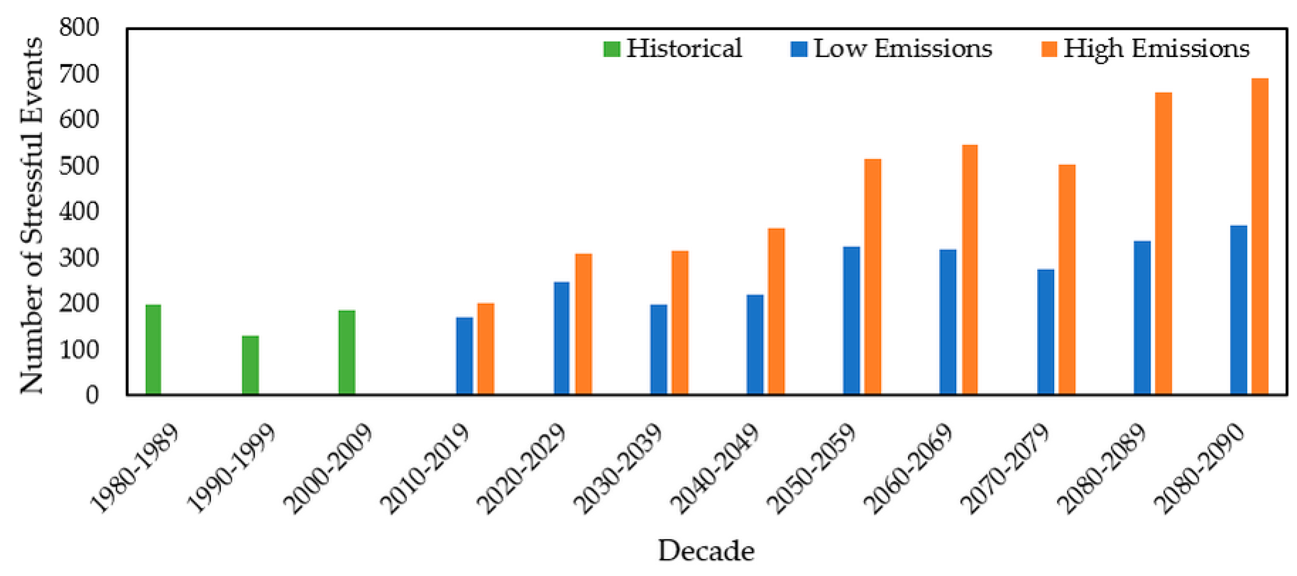
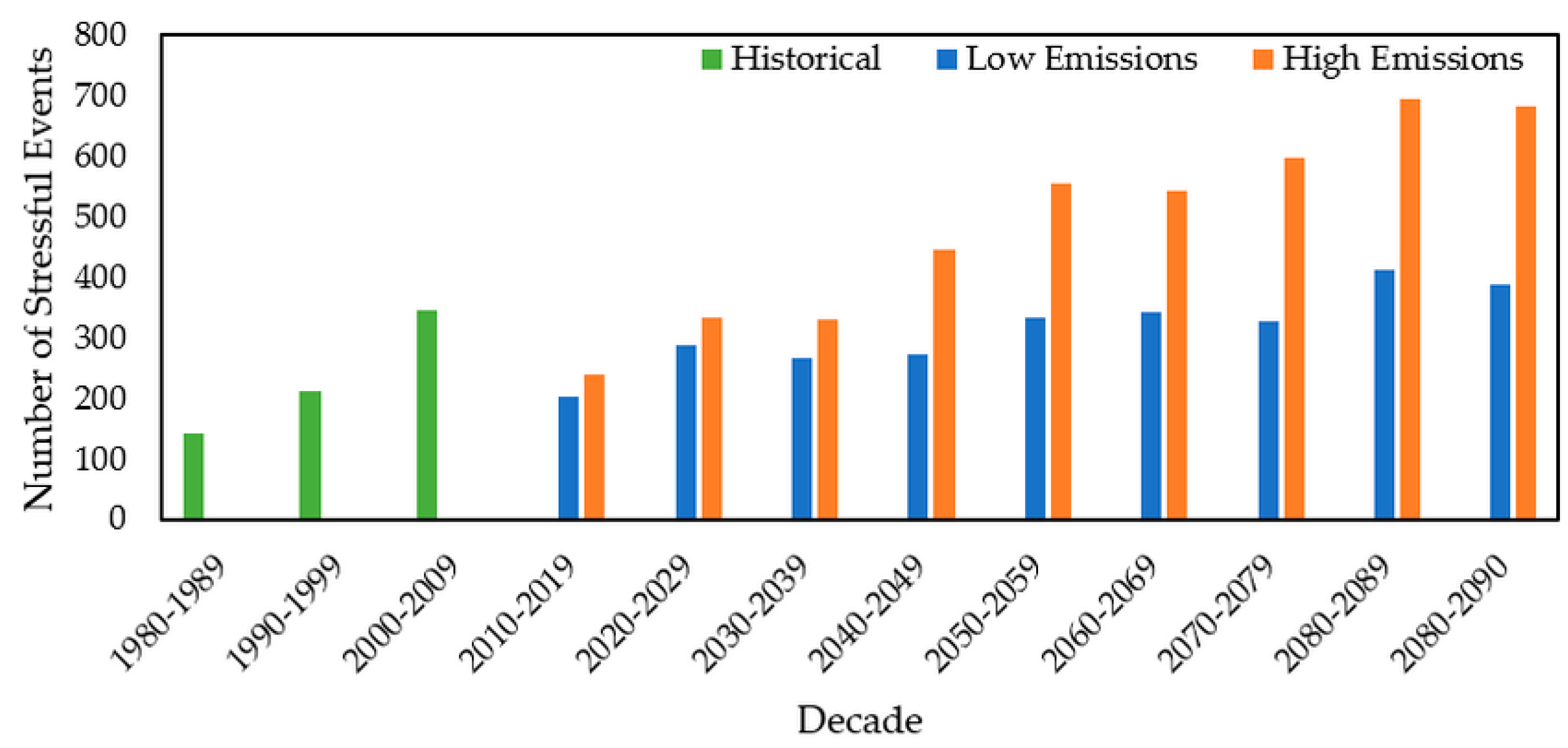
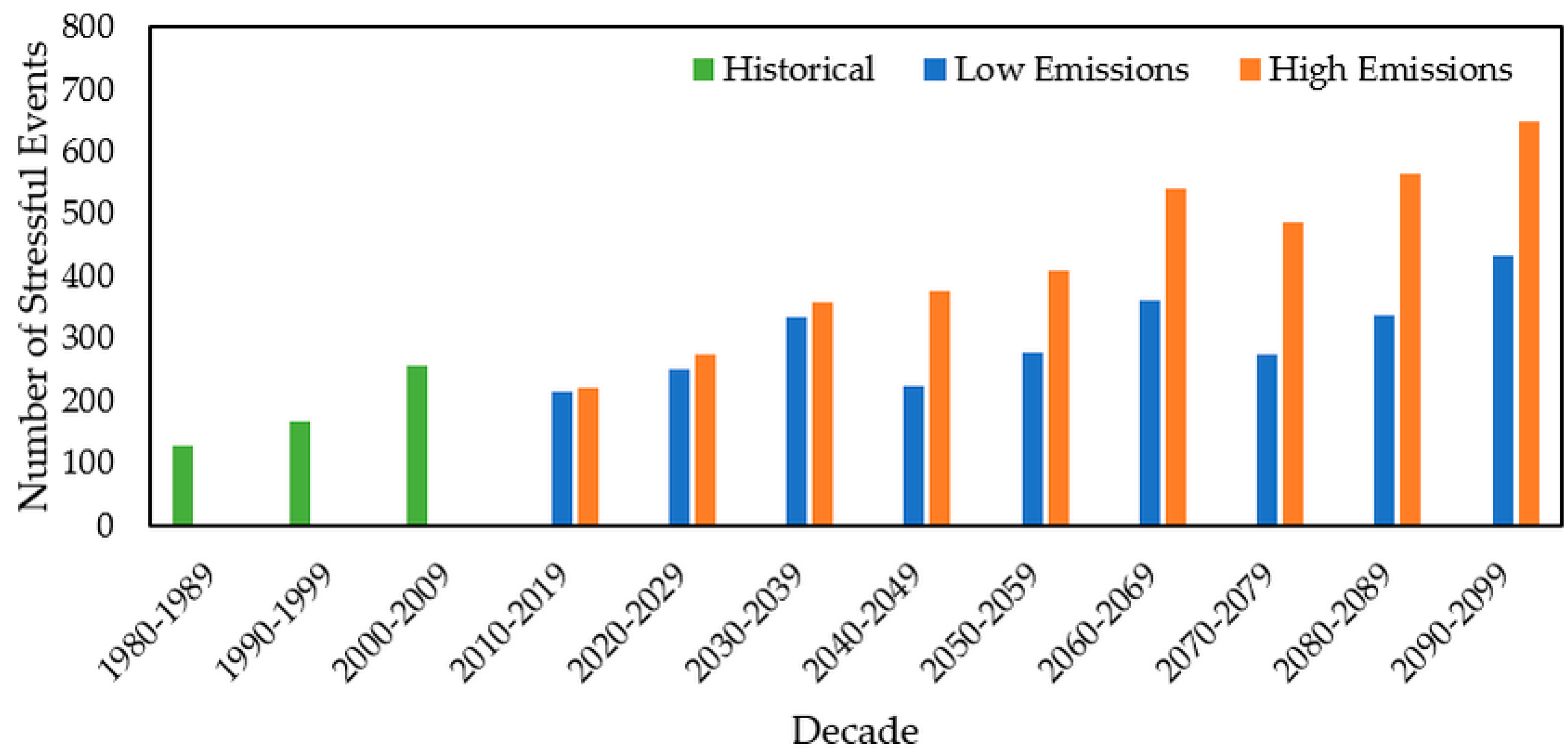
The number of stressful events under the high-emission scenario is greater than the number of events under the low-emission scenario for every decade since 2010, in every watershed (Figure 12, Figure 13 and Figure 14). The graphs also show that for future simulations the number of events in any given decade is higher than the previous decade except for 2060–2069 in the Queen River and 2070–2079 in the Beaver River and Cork Brook. Additionally, it should be noted that there is a minor disconnect between the historical trend and the short-term future simulations; In the Queen River and in Cork Brook Cork there is a higher occurrence between 2000–2009 than there is 2010–2019. The timing of the decrease is likely a result of shifting the model from the regular SWAT code to SWAT with added climate variables, rather than the simulation itself.
Of the three watersheds, the Beaver River and Cork Brook are most likely to provide resilient habitat for brook trout as the local water conditions change due to global warming. Under low-emission scenarios, the Beaver River more frequently displayed the lower percent chance of a stressful event occurring and under the high-emission scenario Cork Brook more frequently had the lowest percent chance by the end of the century. Under both the high- and low-emission scenarios, the chance of stressful events occurring was consistently predicted to be greater in the Queen River. Possible causes of this difference are the larger size of the Queen River watershed and the two tributaries located upstream of the watershed outlet. Fisherville Brook and Queen’s Fort Brook are two waterways that discharge into the Queen River (Figure 1). The Queen’s Fort Brook flows along the eastern side of the watershed through the agricultural area and Fisherville Brook is located along the western side of the watershed where the slope is steeper. Additionally, the main stem of the Queen River itself flows through a large golf course in the middle of the watershed. The tributaries and the main stem come into closer contact with the heterogeneous areas of the basin and may be able to capture additional effects of climate change not seen in the other watersheds. This is not to say that coldwater habitat restoration is not worthwhile in the Queen River, rather that more effort will be needed to restore or maintain brook trout populations in this watershed.
Stream temperatures in all three watersheds were simulated to increase under both low CO2 and high CO2 emission scenarios. It is challenging to discern from this study if stream temperatures in the Beaver River or the Queen River differ significantly because the UGSG gauges at the basin outlet do not record stream temperature and the weather station data used in SWAT simulations was the same for both watersheds. Simulated results do show, however, that stream temperatures will increase through the end of the century by either 1.6 °C under low emissions or 3.4 °C under high emissions in these two watersheds. One-way resource managers can buffer this effect is by preserving existing canopy cover along the riparian corridor. Forest harvesting can increase solar radiation in the riparian zone as well as wind speed and exposure to air advected from clearings, typically causing increases in stream water temperature regimes [87,88]. Additionally, managers may also advocate for preserving groundwater resources that discharge to the streams because baseflow will help regulate stream temperatures, especially if the global low CO2 emission scenario is achieved.

4. Conclusions and Future Work

To help managers identify which areas within a watershed are in the greatest need of protection, a subbasin analysis could be conducted. For instance, both Wood-Pawcatuck basins are home to small preserves managed by The Nature Conservancy. Setting up the model so that a subbasin outlet (as opposed to the watershed outlet) is located within each preserve will allow for assessing site specific conditions when it is not practical to create a model on a small scale. If model output shows that historically these preserves have changed very little, and that future simulations predict minimal change, then managers can put efforts and financial resources towards other preserves that are in greater need.
Another consideration for future work is to limit the stressful event analysis to the spring and summer months when brook trout are more sensitive to warmer stream temperatures. Also, a study could be conducted to see if stressful events occur sequentially. This study took a wider approach by examining how stream temperatures and streamflow vary throughout the entire year. This timeframe was chosen for several reasons. First, since this is the only study of its kind within these watersheds we did not have enough information to say with certainty that no changes to stream temperature or streamflow would occur during the fall and winter. In fact, some scientists predict that by the end of the century Rhode Island will have a climate similar to that of South Carolina and Georgia [26], in which case stream temperatures would almost certainly increase during the winter months. Second, while stream temperatures and streamflow during the winter months are not as critical for brook trout compared to the summer, winter conditions do effect embryo development. For instance, the length of embryo incubation during the winter ranges from 28 to 45 days depending on the temperature of the stream water [12]. Lastly, while this study focused on brook trout, our hope is that the methodology can be applied to other types of aquatic species that may be sensitive to stream conditions during other seasons.
Finally, since all three of these watersheds are baseflow driven, using a model approach that considers the influence of groundwater discharges on stream temperatures would be valuable. A study conducted by Ficklin et al. developed a hydroclimatological SWAT component that incorporates the effects of both air temperatures and hydrological inputs, such as groundwater, on stream temperatures. Previous studies have shown that the hydroclimatological component can be used in small watersheds [89] and in New England [90]. Since the hydroclimatological model component takes the groundwater temperature into consideration, the stream reach will receive inputs that are less exposed to ambient air and therefore cooler during the summer and slightly warmer than the air during the winter. Using a SWAT model with this component may produce more accurate stream temperature results in streams that are baseflow driven.
The purpose of this study was to gain a better understanding of the effects of climate change on coldwater habitat using SWAT. We successfully showed that SWAT can be used to simulate both historical and future climate scenarios in forested, baseflow-driven watersheds in Rhode Island. Moreover, thermally stressful event identification can be a functional approach to analyzing model output. The results indicate that climate change will have a negative effect on coldwater fish species in these types of ecosystems, and that the resiliency of local populations will be tested as stream conditions will likely become increasingly stressful.

Acknowledgments

A thank you to Thomas Boving of the University of Rhode Island and Jameson Chace of Salve Regina University for their insight and review of this Master’s thesis project. We would also like to thank Khurshid Jahan for her help organizing the stream temperature data and creating a template for data processing. We would also like to thank S-1063 Multistate Hatch Grant for supporting this research.

Author Contributions

B.M.C. and S.M.P. conceived and designed the experiments; B.M.C. performed the experiments; B.M.C., S.M.P. and A.J.G. analyzed the data; B.M.C. wrote the paper.

Conflicts of Interest

The authors declare no conflict of interest.

Appendix A

Table A1. Stressful event results for each watershed by decade. High and low CO2 emission scenarios projected for short (2010–2039), medium (2040–2069) and long-term (2070–2099). Unchanged historical results included for reference.
DateEmission ScenarioUnitBeaverQueenCork
1980–1989LowDays200141127
% Chance5.5%3.9%3.5%
HighDays200141127
% Chance5.5%3.9%3.5%
1990–1999LowDays130213168
% Chance3.6%5.8%4.6%
HighDays130213168
% Chance3.6%5.8%4.6%
2000–2009LowDays185346256
% Chance5.1%9.5%7.0%
HighDays185346256
% Chance5.1%9.5%7.0%
2010–2019LowDays172141216
% Chance4.7%3.9%5.9%
HighDays203238221
% Chance5.6%6.5%6.0%
2020–2029LowDays249213252
% Chance6.8%5.8%6.9%
HighDays308334276
% Chance8.4%9.1%7.6%
2030–2039LowDays200346335
% Chance5.5%9.5%9.2%
HighDays317330358
% Chance8.7%9.0%9.8%
2040–2049LowDays221273223
% Chance6.0%7.5%6.1%
HighDays364445375
% Chance10.0%12.2%10.0%
2050–2059LowDays325334278
% Chance8.9%9.1%7.6%
HighDays516555410
% Chance14.1%15.2%11.0%
2060–2069LowDays320343363
% Chance8.8%9.4%9.9%
HighDays547543540
% Chance15.0%14.9%14.8%
2070–2079LowDays276326276
% Chance7.6%8.9%7.6%
HighDays502597487
% Chance13.7%16.3%13.3%
2080–2089LowDays337412338
% Chance9.2%11.3%9.3%
HighDays662694566
% Chance18.1%19.0%15.5%
2090–2099LowDays370389433
% Chance10.1%10.6%11.9%
HighDays692682649
% Chance18.9%18.7%17.8%

References

  1. Hodgkins, G.A.; Dudley, R.W.; Huntington, T.G. Changes in the timing of high river flows in New England over the 20th Century. J. Hydrol. 2003, 278, 244–252. [Google Scholar] [CrossRef]
  2. Eaton, J.G.; Scheller, R.M. Effects of climate warming on fish thermal habitat in streams of the United States. Limnol. Oceanogr. 1996, 41, 1109–1115. [Google Scholar] [CrossRef]
  3. Hayhoe, K.; Wake, C.; Anderson, B.; Liang, X.-Z.; Maurer, E.; Zhu, J.; Bradbury, J.; DeGaetano, A.; Stoner, A.M.; Wuebbles, D. Regional climate change projections for the Northeast USA. Mitig. Adapt. Strateg. Glob. Chang. 2008, 13, 425–436. [Google Scholar] [CrossRef]
  4. Hayhoe, K.; Wake, C.P.; Huntington, T.G.; Luo, L.; Schwartz, M.D.; Sheffield, J.; Wood, E.; Anderson, B.; Bradbury, J.; DeGaetano, A.; et al. Past and future changes in climate and hydrological indicators in the US Northeast. Clim. Dyn. 2007, 28, 381–407. [Google Scholar] [CrossRef]
  5. Mohseni, O.; Erickson, T.R.; Stefan, H.G. Sensitivity of stream temperatures in the United States to air temperatures projected under a global warming scenario. Water Resour. Res. 1999, 35, 3723–3733. [Google Scholar] [CrossRef]
  6. Woodward, G.; Perkins, D.M.; Brown, L.E. Climate change and freshwater ecosystems: Impacts across multiple levels of organization. Philos. Trans. R. Soc. B Biol. Sci. 2010, 365, 2093–2106. [Google Scholar] [CrossRef] [PubMed]
  7. Whitney, J.E.; Al-Chokhachy, R.; Bunnell, D.B.; Caldwell, C.A.; Cooke, S.J.; Eliason, E.J.; Rogers, M.; Lynch, A.J.; Paukert, C.P. Physiological basis of climate change impacts on North American Inland Fishes. Fisheries 2016, 41, 332–345. [Google Scholar] [CrossRef]
  8. Van Vliet, M.T.H.; Franssen, W.H.P.; Yearsley, J.R.; Ludwig, F.; Haddeland, I.; Lettenmaier, D.P.; Kabat, P. Global river discharge and water temperature under climate change. Glob. Environ. Chang. 2013, 23, 450–464. [Google Scholar] [CrossRef]
  9. Jiménez Cisneros, B.E.; Oki, T.; Arnell, N.W.; Benito, G.; Cogley, J.G.; Doll, P.; Jiang, T.; Mwakalila, S.S. 2014: Freshwater resources. In Climate Change 2014: Impacts, Adaptation and Vulnerability. Part A: Global and Sectoral Aspects. Contribution of Working Group II to the Fifth Assessment Report of the Intergovernmental Panel on Climate Change; Kundzewicz, Z., Ed.; Cambridge University Press: Cambridge, UK; New York, NY, USA, 2014; Volume 40. [Google Scholar]
  10. Brett, J.R. Some principles in the thermal requirements of fishes. Q. Rev. Biol. 1956, 31, 75–87. [Google Scholar] [CrossRef]
  11. Fry, F.E.J. The effect of environmental factors on the physiology of fish. In Fish Physiology; Hoar, W.S., Randall, D.J., Eds.; Academic Press: Cambridge, MA, USA, 1971; pp. 1–98. [Google Scholar]
  12. Raleigh, R.F. Habitat Suitability Index Models: Brook trout. In FWS/OBS; United States Fish and Wildlife Service: Washington, DC, USA, 1982. [Google Scholar]
  13. Hokanson, K.E.F.; McCormick, J.H.; Jones, B.R.; Tucker, J.H. Thermal requirements for maturation, spawning, and embryo survival of the brook trout, salvelinus fontinalis. J. Fish. Res. Board Can. 1973, 30, 975–984. [Google Scholar] [CrossRef]
  14. Milner, N.J.; Elliott, J.M.; Armstrong, J.D.; Gardiner, R.; Welton, J.S.; Ladle, M. The natural control of salmon and trout populations in streams. Fish. Res. 2003, 62, 111–125. [Google Scholar] [CrossRef]
  15. Peterson, J.T.; Kwak, T.J. Modeling the effects of land use and climate change on riverine smallmouth bass. Ecol. Appl. 1999, 9, 1391–1404. [Google Scholar] [CrossRef]
  16. Goniea, T.M.; Keefer, M.L.; Bjornn, T.C.; Peery, C.A.; Bennett, D.H.; Stuehrenberg, L.C. Behavioral thermoregulation and slowed migration by adult fall chinook salmon in response to high columbia river water temperatures. Trans. Am. Fish. Soc. 2006, 135, 408–419. [Google Scholar] [CrossRef]
  17. Arnold, J.G.; Srinivasan, R.; Muttiah, R.S.; Williams, J.R. Large area hydrologic modeling and assessment part I: Model development 1. JAWRA J. Am. Water Resour. Assoc. 1998, 34, 73–89. [Google Scholar] [CrossRef]
  18. Isaak, D.J.; Wollrab, S.; Horan, D.; Chandler, G. Climate change effects on stream and river temperatures across the northwest U.S. from 1980–2009 and implications for salmonid fishes. Clim. Chang. 2012, 113, 499–524. [Google Scholar] [CrossRef]
  19. Luo, Y.; Ficklin, D.L.; Liu, X.; Zhang, M. Assessment of climate change impacts on hydrology and water quality with a watershed modeling approach. Sci. Total Environ. 2013, 450, 72–82. [Google Scholar] [CrossRef] [PubMed]
  20. Mohseni, O.; Stefan, H.G. Stream temperature/air temperature relationship: A physical interpretation. J. Hydrol. 1999, 218, 128–141. [Google Scholar] [CrossRef]
  21. Null, S.; Viers, J.; Deas, M.; Tanaka, S.; Mount, J. Stream temperature sensitivity to climate warming in California’s Sierra Nevada. In AGU Fall Meeting Abstracts; Utah State University: Logan, UT, USA, 2010. [Google Scholar]
  22. Preud’homme, E.B.; Stefan, H.G. Relationship between Water Temperatures and Air Temperatures for Central US Streams; St. Anthony Falls Hydraulic Lab, Minnesota University: Minneapolis, MN, USA, 1992; 146p. [Google Scholar]
  23. Anandhi, A.; Frei, A.; Pierson, D.C.; Schneiderman, E.M.; Zion, M.S.; Lounsbury, D.; Matonse, A.H. Examination of change factor methodologies for climate change impact assessment. Water Resour. Res. 2011, 47, 1–10. [Google Scholar] [CrossRef]
  24. Saila, S.; Cheeseman, M.; Poyer, D. Maximum Stream Temperature Estimation from Air Temperature Data and Its Relationship to Brook Trout (Salvelinus Fontinalis) Habitat Requirements in Rhode Island; Wood-Pawcatuck Watershed Association: Hope Valley, RI, USA, 2004. [Google Scholar]
  25. Mohseni, O.; Stefan, H.G.; Eaton, J.G. Global warming and potential changes in fish habitat in U.S. Streams. Clim. Chang. 2003, 59, 389–409. [Google Scholar] [CrossRef]
  26. Climate Solutions New England. Rhode Island’s Climate Past and Future Changes; Sustainability Institute at the University of New Hampshire: Durham, NH, USA, 2016; Available online: http://clim-map.csrcdev.com/files/Rhode%20Island%20(Total)%20Fact%20Sheet.pdf (accessed on 1 March 2017).
  27. Wake, C.; Large, S. Climate Grids for Rhode Island; Sustainability Institute at the University of New Hampshire: Durham, NH, USA, 2014; Available online: clim-map.csrcdev.com/files/Rhode%20Island%20(Total)%20Climate%20Grids.pdf (accessed on 1 March 2017).
  28. Wake, C.P.; Keeley, C.; Burakowski, E.; Wilkinson, P.; Hayhoe, K.; Stoner, A.; LaBrance, J. Climate Change in Northern New Hampshire: Past, Present and Future; Sustainability Institute at the University of New Hampshire: Durham, NH, USA, 2014; Available online: http://scholars.unh.edu/sustainability (accessed on 1 March 2017).
  29. Erkan, D.E. Strategic Plan for the Restoration of Anadromous Fishes to Rhode Island Coastal Streams; Rhode Island Department of Environmental Management, Division of Fish and Wildlife: Wakefield, RI, USA, 2002. [Google Scholar]
  30. WPWA; Saila, S.; Cheeseman, M.; Poyer, D. Assessing Habitat Requirements for Brook Trout (Salvelinus fontinalis) in Low Order Streams; Wood-Pawcatuck Watershed Association: Hope Valley, RI, USA, 2004. [Google Scholar]
  31. Hakala, J.P.; Hartman, K.J. Drought effect on stream morphology and brook trout (Salvelinus fontinalis) populations in forested headwater streams. Hydrobiologia 2004, 515, 203–213. [Google Scholar] [CrossRef]
  32. Bjornn, T.; Reiser, D. Habitat requirements of salmonids in streams. Am. Fish. Soc. Spec. Publ. 1991, 19, 138. [Google Scholar]
  33. Chadwick, J.J.G.; Nislow, K.H.; McCormick, S.D. Thermal onset of cellular and endocrine stress responses correspond to ecological limits in brook trout, an iconic cold-water fish. Conserv. Physiol. 2015, 3, cov017. [Google Scholar] [CrossRef] [PubMed]
  34. Lee, R.M.; Rinne, J.N. Critical thermal maxima of five trout species in the southwestern United States. Trans. Am. Fish. Soc. 1980, 109, 632–635. [Google Scholar] [CrossRef]
  35. Letcher, B.H.; Nislow, K.H.; Coombs, J.A.; O’Donnell, M.J.; Dubreuil, T.L. Population response to habitat fragmentation in a stream-dwelling brook trout population. PLoS ONE 2007, 2, e1139. [Google Scholar] [CrossRef] [PubMed]
  36. Kling, G.W.; Hayhoe, K.; Johnson, L.B.; Magnuson, J.J.; Polasky, S.; Robinson, S.K.; Shuter, B.J.; Wander, M.M.; Wuebbles, D.J.; Zak, D.R. Confronting Climate Change in the Great Lakes Region: Impacts on Our Communities and Ecosystems; Union of Concerned Scientists: Cambridge, MA, USA; Ecological Society of America: Washington, DC, USA, 2003; p. 92. [Google Scholar]
  37. Magnuson, J.J.; Crowder, L.B.; Medvick, P.A. Temperature as an ecological resource. Am. Zool. 1979, 19, 331–343. [Google Scholar] [CrossRef]
  38. Vannote, R.L.; Minshall, G.W.; Cummins, K.W.; Sedell, J.R.; Cushing, C.E. The river continuum concept. Can. J. Fish. Aquat. Sci. 1980, 37, 130–137. [Google Scholar] [CrossRef]
  39. Bunn, S.E.; Arthington, A.H. Basic principles and ecological consequences of altered flow regimes for aquatic biodiversity. Environ. Manag. 2002, 30, 492–507. [Google Scholar] [CrossRef]
  40. Freeman, M.C.; Pringle, C.M.; Jackson, C.R. Hydrologic connectivity and the contribution of stream headwaters to ecological integrity at regional scales1. JAWRA J. Am. Water Resour. Assoc. 2007, 43, 5–14. [Google Scholar] [CrossRef]
  41. Poff, N.L.; Allan, J.D. Functional organization of stream fish assemblages in relation to hydrological variability. Ecology 1995, 76, 606–627. [Google Scholar] [CrossRef]
  42. Poff, N.L.; Allan, J.D.; Bain, M.B.; Karr, J.R.; Prestegaard, K.L.; Richter, B.D.; Sparks, R.E.; Stromberg, J.C. The natural flow regime. Bioscience 1997, 47, 769–784. [Google Scholar] [CrossRef]
  43. Bassar, R.D.; Letcher, B.H.; Nislow, K.H.; Whiteley, A.R. Changes in seasonal climate outpace compensatory density-dependence in eastern brook trout. Glob. Chang. Biol. 2016, 22, 577–593. [Google Scholar] [CrossRef] [PubMed]
  44. DePhilip, M.; Moberg, T. Ecosystem Flow Recommendations for the Susquehanna River Basin; The Nature Conservancy: Harrisburg, PA, USA, 2010. [Google Scholar]
  45. Nuhfer, A.J.; Zorn, T.G.; Wills, T.C. Effects of reduced summer flows on the brook trout population and temperatures of a groundwater-influenced stream. Ecol. Freshw. Fish 2017, 26, 108–119. [Google Scholar] [CrossRef]
  46. Walters, A.W.; Post, D.M. An experimental disturbance alters fish size structure but not food chain length in streams. Ecology 2008, 89, 3261–3267. [Google Scholar] [CrossRef] [PubMed]
  47. Saila, S.; Burgess, D.; Cheeseman, M.; Fisher, K.; Clark, B. Interspecific Association, Diversity, and Population Analysis of Fish Species in the Wood-Pawcatuck Watershed; Wood-Pawcatuck Watershed Association: Hope Valley, RI, USA, 2003. [Google Scholar]
  48. Fulweiler, R.W.; Nixon, S.W. Export of nitrogen, phosphorus, and suspended solids from a southern New England watershed to little Narragansett bay. Biogeochemistry 2005, 76, 567–593. [Google Scholar] [CrossRef]
  49. Poyer, D.; Hetu, M. Study of Maximum Daily Stream Temperature of Select Streams in the Pawcatuck Watershed Summer 2005; Wood-Pawcatuck Watershed Association: Hope Valley, RI, USA, 2005. [Google Scholar]
  50. Dickerman, D.C.; Ozbilgin, M.M. Hydrogeology, water quality, and ground-water development alternatives in the Beaver-Pasquiset ground-water reservoir, Rhode Island. In Water-Resources Investigations Report; US Geological Survey: Reston, VA, USA, 1985. [Google Scholar]
  51. Kliever, J.D. Hydrologic data for the Usquepaug-Queen river basin, Rhode Island. In Open-File Report; US Geological Survey: Reston, VA, USA, 1995. [Google Scholar]
  52. Liu, T.; Merrill, N.H.; Gold, A.J.; Kellogg, D.Q.; Uchida, E. Modeling the production of multiple ecosystem services from agricultural and forest landscapes in Rhode Island. Agric. Resour. Econ. Rev. 2013, 42, 251–274. [Google Scholar] [CrossRef]
  53. Poyer, D.; Hetu, M. Maximum Daily Stream Temperature in the Queen River Watershed and Mastuxet Brook Summer 2006; Wood-Pawcatuck Watershed Association: Hope Valley, RI, USA, 2006. [Google Scholar]
  54. The Nature Conservancy (TNC). Beaver River Preserve. Places We Protect 2017; The Nature Conservancy Is a Nonprofit, Charitable Organization under Section 501(c)(3). Available online: https://www.nature.org/ourinitiatives/regions/northamerica/unitedstates/rhodeisland/placesweprotect/beaver-river-preserve.xml (accessed on 1 May 2017).
  55. Armstrong, D.S.; Parker, G.W. Assessment of Habitat and Streamflow Requirements for Habitat Protection, Usquepaug-Queen River, Rhode Island, 1999–2000; USGS, Ed.; DTIC Document; DTIC: Denver, CO, USA, 2003.
  56. Tefft, E. Factors affecting the distribution of brook trout (salvelinus fontinalis) in the wood-pawcatuck watershed of Rhode Island. In Department of Natural Resources; University of Rhode Island: Kingston, RI, USA, 2013. [Google Scholar]
  57. The Nature Conservancy (TNC). Queen’s River Preserve. Places We Protect 2017; The Nature Conservancy Is a Nonprofit, Charitable Organization under Section 501(c)(3). Available online: https://www.nature.org/ourinitiatives/regions/northamerica/unitedstates/rhodeisland/placesweprotect/queens-river-preserve.xml (accessed on 1 May 2017).
  58. US Geological Survey (USGS). National Water Information System Web Interface; US Geological Survey: Reston, VA, USA, 2017.
  59. Arnold, J.G.; Allen, P.M. Automated methods for estimating baseflow and ground water recharge from streamflow records. JAWRA J. Am. Water Resour. Assoc. 1999, 35, 411–424. [Google Scholar] [CrossRef]
  60. Douglas-Mankin, K.R.; Srinivasan, R.; Arnold, J.G. Soil and Water Assessment Tool (SWAT) Model: Current developments and applications. Trans. ASABE 2010, 53, 1423–1431. [Google Scholar] [CrossRef]
  61. Gassman, P.W.; Reyes, M.R.; Green, C.H.; Arnold, J.G. The soil and water assessment tool: Historical development, applications, and future research directions. Trans. ASABE 2007, 50, 1211–1250. [Google Scholar] [CrossRef]
  62. Neitsch, S.L.; Arnold, J.G.; Kiniry, J.R.; Williams, J.R. Soil and Water Assessment Tool Theoretical Documentation Version 2009; Texas Water Resources Institute: College Station, TX, USA, 2011. [Google Scholar]
  63. Penman, H.L. Estimating evaporation. EOS Trans. Am. Geophys. Union 1956, 37, 43–50. [Google Scholar] [CrossRef]
  64. Monteith, J.L. Evaporation and environment. Symp. Soc. Exp. Biol. 1965, 19, 4. [Google Scholar]
  65. Stefan, H.G.; Preud’homme, E.B. Stream Temperature estimation from air temperature. JAWRA J. Am. Water Resour. Assoc. 1993, 29, 27–45. [Google Scholar] [CrossRef]
  66. RIGIS. Rhode Island Geographic Information System; University of Rhode Island: Kingston, RI, USA, 2016. [Google Scholar]
  67. Texas A&M University. Arcswat Software; Texas A&M University: College Station, TX, USA, 2012; Available online: http://swat.tamu.edu/ (accessed on 19 Octorber 2012).
  68. Homer, C.G.; Dewitz, J.A.; Yang, L.; Jin, S.; Danielson, P.; Xian, G.; Coulston, J.; Herold, N.D.; Wickham, J.; Megown, K. Completion of the 2011 National Land Cover Database for the conterminous United States-Representing a decade of land cover change information. Photogramm. Eng. Remote Sens. 2015, 81, 345–354. [Google Scholar]
  69. Rhode Island Geographic Information System (RIGIS) Data Distribution System SOIL_Soils. Available online: http://www.rigis.org/geodata/soil/Soils16.zip (accessed on 5 September 2016).
  70. Saha, S.; Moorthi, S.; Wu, X.; Wang, J.; Nadiga, S.; Tripp, P.; Behringer, D.; Hou, Y.-T.; Chuang, H.-Y.; Iredell, M.; et al. The NCEP climate forecast system version 2. J. Clim. 2014, 27, 2185–2208. [Google Scholar] [CrossRef]
  71. Texas A&M, U. NCEP Global Weather Data for Swat. Available online: https://globalweather.tamu.edu (accessed on 3 January 2016).
  72. Abbaspour, K.C. SWAT-CUP 2012; SWAT Calibration and Uncertainty Program—A User Manual; Swiss Federal Institute of Aquatic Science and Technology Eawag: Duebendorf, Switzerland, 2013. [Google Scholar]
  73. Abbaspour, K. User Manual for SWAT-CUP, SWAT Calibration and Uncertainty Analysis Programs; Swiss Federal Institute of Aquatic Science and Technology Eawag: Duebendorf, Switzerland, 2007. [Google Scholar]
  74. Nash, J.E.; Sutcliffe, J.V. River flow forecasting through conceptual models part I—A discussion of principles. J. Hydrol. 1970, 10, 282–290. [Google Scholar] [CrossRef]
  75. Moriasi, D.N.; Arnold, J.G.; Liew, M.W.V.; Bingner, R.L.; Harmel, R.D.; Veith, T.L. Model evaluation guidelines for systematic quantification of accuracy in watershed simulations. Trans. ASABE 2007, 50, 885–900. [Google Scholar] [CrossRef]
  76. Pradhanang, S.M.; Mukundan, R.; Schneiderman, E.M.; Zion, M.S.; Anandhi, A.; Pierson, D.C.; Frei, A.; Easton, Z.M.; Fuka, D.; Steenhuis, T.S. Streamflow responses to climate change: Analysis of hydrologic indicators in a New York City water supply watershed. J. Am. Water Resour. Assoc. 2013, 49, 1308–1326. [Google Scholar] [CrossRef]
  77. Liew, M.W.V.; Veith, T.L.; Bosch, D.D.; Arnold, J.G. Suitability of SWAT for the conservation effects assessment project: Comparison on USDA agricultural research service watersheds. J. Hydrol. Eng. 2007, 12, 173–189. [Google Scholar] [CrossRef]
  78. Arnold, J.G.; Allen, P.M.; Muttiah, R.; Bernhardt, G. Automated base flow separation and recession analysis techniques. Ground Water 1995, 33, 1010–1018. [Google Scholar] [CrossRef]
  79. Singh, J.; Knapp, H.V.; Arnold, J.G.; Demissie, M. Hydrological modeling of the Iroquois river watershed using HSPF and SWAT. JAWRA J. Am. Water Resour. Assoc. 2005, 41, 343–360. [Google Scholar] [CrossRef]
  80. Pyrce, R. Hydrological Low Flow Indices and Their Uses; Watershed Science Centre (WSC) Report; Watershed Science Center, Trent University: Peterborough, ON, Canada, 2004. [Google Scholar]
  81. Smakhtin, V.U. Low flow hydrology: A review. J. Hydrol. 2001, 240, 147–186. [Google Scholar] [CrossRef]
  82. Ahearn, E.A. Flow Durations, Low-Flow Frequencies, and Monthly Median Flows for Selected Streams in Connecticut through 2005; US Department of the Interior, US Geological Survey: Reston, VA, USA, 2008. [Google Scholar]
  83. Demaria, E.M.C.; Palmer, R.N.; Roundy, J.K. Regional climate change projections of streamflow characteristics in the Northeast and Midwest U.S. J. Hydrol. Reg. Stud. 2016, 5, 309–323. [Google Scholar] [CrossRef]
  84. Douglas, E.M.; Vogel, R.M.; Kroll, C.N. Trends in floods and low flows in the United States: Impact of spatial correlation. J. Hydrol. 2000, 240, 90–105. [Google Scholar] [CrossRef]
  85. Ficklin, D.L. SWAT Stream Temperature Executable Code; Indiana State University: Terre Haute, IN, USA, 2012. [Google Scholar]
  86. Meisner, J.D.; Rosenfeld, J.S.; Regier, H.A. The role of groundwater in the impact of climate warming on stream salmonines. Fisheries 1988, 13, 2–8. [Google Scholar] [CrossRef]
  87. Moore, R.D.; Spittlehouse, D.L.; Story, A. Riparian microclimate and stream temperature response to forest harvesting: A Review. J. Am. Water Resour. Assoc. 2005, 41, 813–834. [Google Scholar] [CrossRef]
  88. Rishel, G.B.; Lynch, J.A.; Corbett, E.S. Seasonal stream temperature changes following forest harvesting. J. Environ. Qual. 1982, 11, 112–116. [Google Scholar] [CrossRef]
  89. Ficklin, D.L.; Luo, Y.; Stewart, I.T.; Maurer, E.P. Development and application of a hydroclimatological stream temperature model within the Soil and Water Assessment Tool. Water Resour. Res. 2012, 48. [Google Scholar] [CrossRef]
  90. Brennan, L. Stream Temperature Modeling: A modeling comparison for resource managers and climate change analysis. In Environmental and Water Resources Engineering; University of Massachusetts: Amherst, MA, USA, 2015. [Google Scholar]
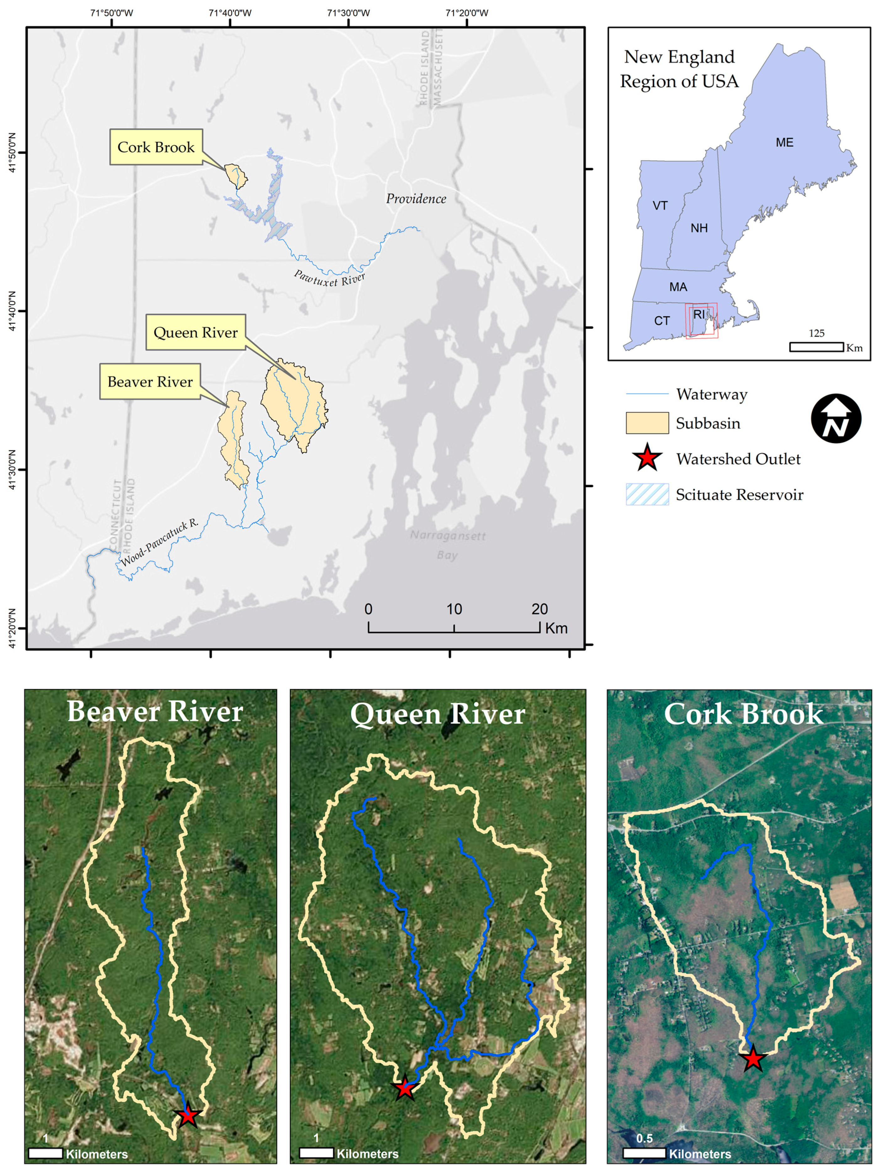
Figure 1. The study sites include the Beaver River, Queen River and Cork Brook watersheds in Rhode Island, USA.
Water 09 00732 g001
Figure 2. (a) Hydrograph and (b) scatterplot of observed versus SWAT modeled streamflow at Beaver River USGS gauge 01117468 during calibration years 2000–2005.
Water 09 00732 g002
Figure 3. (a) Hydrograph and (b) scatterplot of observed versus SWAT modeled streamflow at Queen River USGS gauge 01117370 during calibration years 2000–2005.
Water 09 00732 g003aWater 09 00732 g003b
Figure 4. (a) Hydrograph and (b) scatterplot of observed versus SWAT modeled streamflow at Cork Brook USGS gauge 01115280 during calibration years 2009–2010.
Water 09 00732 g004
Figure 5. Beaver River simulated historical flow duration curve and stream temperatures. The secondary y-axis begins at 21 °C and any temperatures that are not above the stressful threshold are not shown in the figure. The stream temperatures in the Q25–Q75 range are omitted from the figure.
Water 09 00732 g005
Figure 6. Queen River simulated historical flow duration curve and stream temperatures. The secondary y-axis begins at 21 °C and any temperatures that are not above the stressful threshold are not shown in the figure. The stream temperatures in the Q25–Q75 range are omitted from the figure.
Water 09 00732 g006
Figure 7. Cork Brook simulated historical flow duration curve and stream temperatures. The secondary y-axis begins at 21 °C and any temperatures that are not above the stressful threshold are not shown in the figure. The stream temperatures in the Q25–Q75 range are omitted from the figure.
Water 09 00732 g007
Figure 8. Beaver River flow duration curves simulated for high and low CO2 emission scenarios by the end of the long-term (2070–2099). Unchanged historical results included for reference.
Water 09 00732 g008
Figure 9. Queen River flow duration curves simulated for high and low CO2 emission scenarios by the end of the long-term (2070–2099). Unchanged historical results included for reference.
Water 09 00732 g009
Figure 10. Cork Brook flow duration curves simulated for high and low CO2 emission scenarios by the end of the long-term (2070–2099). Unchanged historical results included for reference.
Water 09 00732 g010
Figure 11. The number of days per month that stream temperatures exceeded the stress threshold in 1980, 2099 under low CO2 emissions and 2099 under high CO2 emissions in (a) the Beaver and Queen Rivers which had the same weather station and (b) Cork Brook.
Water 09 00732 g011
Figure 12. Number of stressful events predicted in the Beaver River watershed between 1980 and 2099 under historical conditions, low CO2 emissions and high CO2 emission scenarios.
Water 09 00732 g012
Figure 13. Number of stressful events predicted in the Queen River watershed between 1980 and 2099 under historical conditions, low CO2 emissions and high CO2 emission scenarios.
Water 09 00732 g013
Figure 14. Number of stressful events predicted in the Cork Brook watershed between 1980 and 2099 under historical conditions, low CO2 emissions and high CO2 emission scenarios.
Water 09 00732 g014
Table 1. Statistical results of daily streamflow calibration produced by SWAT-CUP.
WatershedR2NSEPBIAS
Beaver River0.640.570.13
Queen River0.580.580.002
Cork Brook0.700.71−0.01
Table 2. Statistical results of daily streamflow validation produced by SWAT-CUP.
StreamflowR2NSEPBIAS
Beaver River0.660.600.13
Queen River0.600.590.003
Cork Brook0.540.500.03
Table 3. Range of values for ten most sensitive parameters during daily streamflow calibration using SWAT-CUP for (a) Beaver River, (b) Queen River and (c) Cork Brook. Parameters are listed by name and SWAT input file type, definition and the range of values that were selected for the model.
ParameterDefinitionValue RangeUnits
(a) Beaver River parameters for daily streamflow calibration.
CN2.mgtSCS runoff curve number−60–75-
ALPHA_BF.gwBaseflow alpha factor0.0–0.101/Days
GW_DELAY.gwGroundwater delay0.0–10Days
TIMP.bsnSnowpack temperature lag factor−1.5–2.0-
ALPHA_BNK.rteBaseflow alpha factor for bank storage0.50–1.0Days
OV_N.hruManning’s (n) value for overland flow1.0–30-
SLSUBBSN.hruAverage slope length10–50m
(b) Queen River parameters for daily streamflow calibration.
CN2.mgtSCS runoff curve number60–75-
ALPHA_BF.gwBaseflow alpha factor0.0–0.101/Days
GW_REVAP.gwGroundwater revap coefficient0.02–0.15Days
GW_DELAY.gwGroundwater delay0.0–10.0Days
GWQMN.gwDepth of water in shallow aquifer for return flow150–1000mm
TIMP.bsnSnowpack temperature lag factor0.0–1.0-
ALPHA_BNKBaseflow alpha factor for bank storage0.5–1.0Days
(c) Cork Brook parameters for daily streamflow calibration.
CN2.mgtSCS runoff curve number−60–75-
ALPHA_BF.gwBaseflow alpha factor0.0–0.101/Days
GW_DELAY.gwGroundwater delay0.0–7.0Days
GWQMN.gwDepth of water in shallow aquifer for return flow200–1000mm
SMTMP.bsnSnowmelt base temperature−0.5–2.0°C
ESCO.hruSoil evaporation compensation factor0.15–0.65-
EPCO.hruPlant uptake compensation factor0.15–0.65-
SLSOIL.hruSlope length for lateral subsurface flow0.0–150.0m
Table 4. Climate change variables adopted and modified from Wake et al., 2014 [27] for (a,b) Kingston, RI (Beaver River and Queen River) and (c,d) North Foster, RI (Cork Brook). Low emissions (a,c) based on SRES A1fi scenario and high emissions (b,c) based on SRES B1 scenario. Temperatures (Temp.) listed as degree (°C) increase, averaged from the published minimum and maximum temperatures. Precipitation (Precip.) values listed as a relative change computed based on the published values.
IndicatorJanuaryFebruaryMarchAprilMayJuneJulyAugustSeptemberOctoberNovemberDecember
(a) Low Emissions–Kingston, RI
Short-term Temp. 0.970.971.421.421.420.830.830.830.360.360.360.97
Med-term Temp. 1.501.502.472.472.471.581.581.580.560.560.561.50
Long-term Temp. 2.172.173.253.253.251.971.971.970.830.830.832.17
Short-term Precip. 8.768.769.809.809.8017.917.917.95.595.595.598.76
Med-term Precip. 14.314.310.310.310.317.917.917.96.906.906.9014.3
Long-term Precip. 14.914.916.316.316.318.618.618.610.610.610.614.9
(b) High Emissions–Kingston, RI
Short-term Temp. 0.970.970.830.830.831.111.111.111.001.001.000.97
Med-term Temp. 2.222.222.362.362.363.063.063.063.003.003.002.22
Long-term Temp. 3.833.834.284.284.285.225.225.224.924.924.923.83
Short-term Precip. 8.098.0914.214.214.212.512.512.54.934.934.938.09
Med-term Precip. 10.010.015.815.815.812.512.512.56.26.26.210.0
Long-term Precip. 22.322.322.022.022.010.210.210.28.168.168.1622.3
(c) Low Emissions–North Foster, RI
Short-term Temp. 1.001.001.421.421.420.970.970.970.390.390.391.00
Med-term Temp. 1.581.582.532.532.531.811.811.810.580.580.582.22
Long-term Temp. 2.222.223.333.333.332.252.252.250.810.810.812.22
Short-term Precip. 10.610.611.311.311.316.916.916.96.626.626.6210.6
Med-term Precip.12.912.911.911.911.917.417.417.410.110.110.112.9
Long-term Precip. 16.216.215.615.615.617.417.417.411.811.811.816.2
(d) High Emissions–North Foster, RI
Short-term Temp. 0.970.970.890.890.891.221.221.220.890.890.890.97
Med-term Temp. 2.222.222.502.502.503.283.283.282.782.782.782.22
Long-term Temp. 3.863.864.474.474.475.505.505.504.644.644.643.86
Short-term Precip. 6.296.2910.810.810.815.715.715.72.082.082.086.29
Med-term Precip. 8.848.8411.311.311.318.018.018.02.762.762.768.84
Long-term Precip. 17.717.720.020.020.017.417.417.45.375.375.3717.7
Table 5. The average stream temperature simulated by SWAT 1980–2009.
WatershedAverage Daily Stream Temp. (°C)Average Daily Discharge (m3/s)
Beaver River13.00.38
Queen River13.01.0
Cork Brook12.50.081
Table 6. Stressful event analysis of SWAT simulation for the three study sites.
DateWatershedIndicatorAny Type of StressStream Temp. > 21 °CQ25 or Q75 FlowStressful Event
1980–2009Beaver RiverDays64169595457511
% Chance58.6%8.8%49.8%4.7%
Queen RiverDays65069595547700
% Chance59.4%8.8%50.6%5.5%
Cork BrookDays687514095466551
% Chance62.7%12.9%49.9%4.4%
Table 7. Average stream temperature and streamflow simulated with climate change variables for (a) Beaver River, (b) Queen River and (c) Cork Brook. High and low CO2 emission scenarios projected for short (2010–2039), medium (2040–2069) and long-term (2070–2099). Unchanged historical results included for reference.
ScenarioDateAverage Daily Stream Temp. (°C)Average Daily Discharge (m3/s)
(a)
Beaver River Historical1980–200913.00.38
Beaver River Low Emissions2010–203913.60.44
2040–206914.20.45
2070–209914.60.47
Beaver River High Emissions2010–203913.70.49
2040–206915.00.53
2070–209916.40.65
(b)
Queen River Historical1980–200913.01.0
Queen River Low Emissions2010–203913.61.14
2040–206914.21.16
2070–209914.61.19
Queen River High Emissions2010–203913.71.20
2040–206915.01.27
2070–209916.41.49
(c)
Cork Brook Historical1980–200912.50.081
Cork Brook Low Emissions2010–203913.20.09
2040–206913.250.10
2070–209914.110.10
Cork Brook High Emissions2010–203913.250.10
2040–206914.520.10
2070–209915.970.13
Table 8. Percent chance of a stressful event occurring under future climate scenarios. Results for each watershed by 30-year increments. High and low CO2 emission scenarios projected for short (2010–2039), medium (2040–2069) and long-term (2070–2099). Unchanged historical results included for reference.
DateEmission ScenarioUnitBeaverQueenCork
1980–2009Historical% Chance4.75.54.4
Historical4.75.54.4
2010–2039Low% Chance6.26.96.5
High7.27.97.2
2040–2069Low% Chance7.98.57.1
High12.413.111.3
2079–2099Low% Chance9.09.88.6
High16.116.815.2