Abstract
Spatial surface soil moisture can be an important indicator of crop conditions on farmland, but its continuous estimation remains challenging due to coarse spatial and temporal resolution of existing remotely-sensed products. Furthermore, while preceding research on soil moisture using remote sensing (surface energy balance, weather parameters, and vegetation indices) has demonstrated a relationship between these factors and soil moisture, practical continuous spatial quantification of the latter is still unavailable for use in water and agricultural management. In this study, a methodology is presented to estimate volumetric surface soil moisture by statistical selection from potential predictors that include vegetation indices and energy balance products derived from satellite (Landsat) imagery and weather data as identified in scientific literature. This methodology employs a statistical learning machine called a Relevance Vector Machine (RVM) to identify and relate the potential predictors to soil moisture by means of stratified cross-validation and forward variable selection. Surface soil moisture measurements from irrigated agricultural fields in Central Utah in the 2012 irrigation season were used, along with weather data, Landsat vegetation indices, and energy balance products. The methodology, data collection, processing, and estimation accuracy are presented and discussed.
1. Introduction
The future of agriculture and food security depends, in large measure, on overcoming current and future limitations on development of new irrigation systems, which must become more productive and efficient in order to feed an increasing population [1]. The use of remote sensing techniques to monitor agricultural variables (water, yield, nutrients, etc.) represents an existing information source that can significantly enhance agriculture and water management [1,2,3,4,5]. Soil moisture (or soil water content) is an important variable because, along with evapotranspiration estimates, soil moisture can support estimation of current and future irrigation water needs using water balance techniques [1,6,7,8].
Despite their utility, soil moisture estimations for agricultural applications have proven to be challenging to implement at an operational level because of complex feedback processes that involve factors, such as atmospheric conditions (weather, time of the year), vegetation (actual evapotranspiration, crop canopy structure, irrigation frequency, etc.), and soil characteristics (cover, organic matter, texture, structure, heterogeneity, and root density) [7,9,10]. Another challenge is the spatial and temporal resolution of soil moisture measurements and estimations. Ground sensor measurements (points) can continuously measure soil moisture but are limited in spatial coverage. Available soil moisture measurements based on optical, thermal, and radar satellites provide spatial coverage, but the coarse spatial resolution (pixel size) or untimely information during the irrigation season limit their use for crop field operations [11,12]. Finally, existing land surface models developed for estimation of soil moisture are not necessarily spatial in nature, or they require information not generally available for their calibration [13]. Thus, despite the plethora of available procedures for estimating soil moisture, continuous production of spatially distributed soil water content information for agriculture at adequate spatial and temporal resolutions is not yet possible.
To address the complex nature of soil moisture, statistical learning theory tools such as Artificial Neural Networks (ANNs), Support Vector Machines (SVMs), and Relevance Vector Machines (RVMs), have been tested in recent years for their ability to spatially estimate distributed soil moisture at the single-farm level. A key characteristic of these learning machine algorithms is their use of the underlying statistical characteristics of available information (predictors and predictands) without prior assumptions of their relationship. Examples of learning machine algorithms in spatial applications used in water resources and soil moisture applications can be found in [6,8,14,15,16,17,18,19,20,21], among others. The RVM, a Bayesian regression algorithm, was applied in several of these studies. As a sparse model with high accuracy, RVM has been used in hydrology, water resources, and other fields.
The objective of this study was to develop a methodology for estimating surface soil moisture at adequate spatial and temporal resolution to support management of irrigated fields (Landsat image resolution) by integrating previously identified remote sensing and local information related to soil moisture, such as vegetation indices, energy balance products, and weather data. The RVM learning machine algorithm was used as the modelling tool. An existing surface energy balance model called METRIC™ was used to produce energy balance products. Spatial and ground information collected from an irrigation system in Central Utah for the 2012 irrigation season was used for this study. To the best knowledge of the authors, the current research is the first effort to estimate surface soil moisture at a spatial and temporal resolution by combining different datasets (in situ measurements and remote-sensing products) and suitable modeling techniques based on Landsat vegetation indices, surface energy balance products, and a Bayesian machine learning approach (RVM).
2. Literature Review
2.1. Soil Moisture Measurement and Estimation
Soil moisture plays a key role in a number of water and energy processes that affect weather, vegetation, and global chemical cycles [22]. Additionally, spatial distribution of soil moisture is required for determining hydrological processes, including land–atmospheric interactions, rainfall-runoff response, and erosion processes [23]. In agriculture, estimation of soil moisture content is important for irrigation scheduling, water management, crop growth, yield forecast modeling, forest dynamics, partitioning of sensible, and latent heat fluxes (i.e., Bowen Ratio), and surface-atmospheric interactions, among others [7]. Soil moisture is especially important in precision farming because soil moisture content information for any location within or across fields can provide a clear understanding of current soil water condition; thus, producers/irrigators can more effectively direct their sub-field or zonal water management efforts.
The study of soil moisture in agriculture divides the soil profile into two zones: the surface zone, which covers the first five centimeters (two inches) of soil, and the root zone soil moisture (held in the upper 200 cm of soil) [7,9]. This differentiation is based on the influence of external factors to each zone. The surface zone becomes a physical interface between the atmosphere and the soil water content, which regulates the rate of soil water evaporation. The root zone is strongly influenced by the initial water content and water fluxes from the phreatic water underneath. Surface soil moisture is physically related to the root zone through diffusion processes [7].
In general, soil moisture measurements can be described as point measurements, which can be acquired using gravimetric, nuclear, electromagnetic, tensiometric, and hygrometric techniques or embedded sensors, such as time- and frequency-domain reflectometry (TDRs and FDRs) [7]. These measurements are the most accurate, given the close contact of the sensor to the water-holding medium (soil), and are considered ground truth. Nevertheless, these measurements are restricted in spatial coverage to a small distance from where the sensor is placed. Therefore, installation of a large or dense sensor network would be necessary to monitor large field areas, with the associated inconveniences of operation and maintenance costs, especially in intensively mechanized fields.
Over the past decades, remote sensing technology has shown encouraging results for spatial estimation of soil moisture. Methods applicable on vegetation-covered surfaces have been limited to two basic wavelength bands: thermal infrared and microwave. The use of each band has its special advantages and disadvantages, which often allow the two bands to complement one another.
Microwave techniques, which rely on the large effect of water content on the soil dielectric constant, have the advantage of a wide dynamic range in signal between wet and dry soils. Remote sensing measurements in the microwave region can give useful information about soil moisture, due to the strong contrast between the dielectric constant of dry soil and water (four and 80, respectively) and its effect on microwave emission [24,25,26]. The Soil Moisture Active Passive Satellite Program (SMAP) launched in 2015 was designed to provide direct estimation of surface soil moisture (Product Level 4 Surface and Root Soil Moisture L4_SM) at a resolution of 9 km/pixel by merging active radar information from SMAP with a land surface model [27,28]. Nevertheless, due to its spatial resolution, SMAP and other microwave satellites do not provide information at adequate scales (farm, subfield, ~30m/pixel), thus limiting their application to subbasin and larger scales.
Thermal infrared observation of soil moisture has the advantage of requiring a significantly more modest sensing system. A study of irrigated wheat [29] concluded that useful qualitative soil moisture information could be obtained from vegetation canopy temperature measurements where the soil was completely obscured. In addition, [30] showed that soil moisture can be most accurately estimated by thermal infrared information in dry or marginal agricultural areas where drought is a frequent threat.
In addition to infrared thermal and microwave sensing, other documented research efforts have estimated surface and root soil moisture using optical remote sensing imagery. [31,32,33] present a relationship between root zone soil moisture conditions and the evaporative fraction (crop coefficient) as a product of the Surface Energy Balance Algorithm for Land (SEBAL), using Landsat and MODIS as sources of remotely-sensed data, as long as soil texture is adequately mapped. [6,20,21] found relationships between surface soil moisture and remote sensing indices and products (such as NDVI; SAVI; LAI), surface temperature, meteorological parameters (precipitation, air temperature), and soil water holding capacity. [34,35] found that Landsat reflectance band ratios and cap-tasseled transformations were non-linearly related to surface soil moisture. Vegetation and soil water content have been found to be related to Landsat Normalized Burn Ratio (NBR) [36], as well as surface albedo [37] and energy balance components [38].
Finally, physically-based models for soil moisture estimation, also called land surface models [25,39], relate soil water content and surface fluxes. [20] lists some of these land surface models, which include the Soil-Plant-Atmosphere-Water model [40,41], US Department of Agriculture Hydrograph Laboratory [42,43], Sacramento Soil Moisture Accounting Model [44], and soil vegetation atmosphere transfer schemes [45]. However, the difficulty associated with measuring physical parameters required by these models serves as an impediment for their intensive use in agricultural management [20]. Research on land surface models has confirmed that soil moisture varies both in space and time because of spatial and temporal variations in precipitation, weather patterns, soil, topographic features, and vegetation characteristics [39,46]. Additionally, there is an inherent feedback process between atmosphere and surface soil moisture [9]. Near-surface atmospheric conditions (for example, humidity and temperature) affect the magnitude and direction of surface fluxes as soil moisture, while surface energy and hydrological fluxes affect atmospheric conditions at the surface. Land surface models have identified wind speed, roughness, and biomass as the three more important parameters that have a uniformly large effect on all of the potential signatures and would, therefore, need to be taken into account in any selected soil moisture algorithm [30]. For issues of soil moisture scaling, the confounding effects of atmospheric stability, soil properties, vegetation, and topography also need to be considered. Results from these land surface models suggest that it may be possible to combine some simple parameters relating root zone soil moisture, surface runoff, groundwater discharge, the surface energy budget equation, and the effective evaporation efficiency control to describe the equilibrium state of a land surface scheme [9]. However, issues related to interactions among multiple processes, nonlinearities, and feedbacks across land surfaces, along with relationships among single-sensor measurement, statistical averages, and the definition of spatial heterogeneity within pixels, are yet to be solved.
2.2. The Mapping Evapotranspiration at High Resolution with Internalized Calibration Model (METRIC) Model
The Mapping EvapoTranspiration at high Resolution with Internalized Calibration (METRIC) model is an algorithm developed by [47] to estimate actual evapotranspiration (ET) for agricultural lands using aerial or satellite imagery that includes a thermal band. METRIC has been validated extensively using the Landsat satellite platform [3], and continued research and development of applications demonstrate its validity. One main characteristic of METRIC is its specific design for arid, desert areas, such as the Western US and coastal locations in the world where water availability is restricted and improved water management is necessary. METRIC is based on the Surface Energy Balance (SEB) equation [48,49], the formulation of which is as follows Equation (1):
where Rn is net radiation at the surface; G is the soil heat flux; H is the sensible heat flux to the air; and LE is the latent heat flux (or actual evapotranspiration: the energy used to evaporate water). Every component of the SEB equation is expressed in Watts/m2. ET models such as METRIC, SEBAL, and others, make use of the SEB equation to estimate actual evapotranspiration (LE) by solving for the other three components of Equation (1) [3]. The METRIC model solves for each of the parameters of the SEB equation with the following procedure:
Rn Equation (2) is computed for each pixel using albedo (α) and transmittances computed from short wavebands (Landsat first to fifth and seventh reflectance bands, or ρ1:ρ5 and ρ7), using broadband emissivity (ε0) computed from the thermal band (Landsat sixth band).
where Rs↓, RL↑, and RL↓ are the incoming shortwave, emitted outgoing longwave, and the incoming longwave radiation, respectively (W/m2) [48,50].
Soil heat flux (G, Equation (3)) is predicted using leaf area index (LAI) and surface temperature (Ts), along with the Rn estimates [51]:
Sensible heat (H, Equation (4)) is calculated from several factors: a single wind speed measurement at the ground, air density (ρair), air specific heat (cp), estimated aerodynamic resistance to heat transport (rah), and surface-to-air temperature differences (dT) predicted from thermal infrared radiances.
All computations are made specific to each pixel in the image. Iterative predictions of H are improved using atmospheric stability corrections based on Monin-Obukhov similarity [51]. Endpoints for H within a satellite image are bounded by known evaporative conditions at key reference (anchor) points [50]. These reference points include pixels having little or no evaporation (the “hot pixel”) and maximum evapotranspiration (the “cold pixel”). Evapotranspiration is calculated from LE by dividing by the latent heat of vaporization. Further details of the METRIC algorithm are presented in [3,47,50].
2.3. The Relevance Vector Machine
The relevance vector machine (RVM) is a Bayesian learning approach for supervised learning regression and classification tasks developed by [52] and posteriorly enhanced by [53]. The RVM is a nonlinear model based on a Bayesian probabilistic treatment to determine a descriptive function based on existing information. The RVM has been extensively used in hydrological, water resources, and Earth image processing [6,15,18,19,54,55], with excellent results.
The development of an RVM model for regression tasks is based on a training set of input vectors with corresponding targets . For this training subset, the RVM develops a model of dependency of targets t on the inputs x, thus achieving accurate predictions of t for previously unseen values of x [52]. The general form of the RVM function is presented in Equations (5) and (6):
where w is the model “weights” and Φ(x) is a basis function where Φ=[φ1… φM] is the N * M “design” matrix whose columns comprise the complete set of M “basic vectors”, y or yn is the RVM predictand, and εn is the difference or residual [53]. The main feature of the RVM is the target function y Equation (5), which attempts to minimize the difference ε with respect to t Equation (6).
Two main assumptions are made to implement the Bayesian probabilistic approach in the RVM: the distribution probability of t, p(tn|xn) is Gaussian distributed, N(tn|yn,σ2), as is the difference ε, N(0,σ2). Using these two assumptions, the likelihood of the set {x, t} can be written as:
To avoid overfitting issues when solving for w and σ, usually by maximum likelihood methods [56], a common approach is to impose on them constraints based on an assumed “prior” Gaussian probability distribution Equation (8):
with α being a vector of Q hyperparameters, individually related to each weight value. From Bayes’ rule, the “posterior” probability over all unknown parameters over the set is:
The first part of Equation (9) can be expressed as p(w|t, α,σ2) ∼ N(m, Σ), where the mean m and the covariance Σ are given by:
and A = diag(α). Solving for m and Σ involves finding the hyperparameters (α and σ2) that maximize the second term in Equation (9):
Assuming uniform hyperpriors (thus ignoring p(α) and p(σ2)), it is possible to maximize the evidence or likelihood function (the first term in Equation (12)):
Replacing Equations (7) and (8) while solving the integrand gives:
where:
A fast marginal likelihood optimization algorithm is used to obtain the optimal set of hyperparameters αopt and σopt2 (which affects the estimation of m and Σ). This optimization algorithm uses an efficient sequential addition and deletion of candidate basis functions described by [53]. Thus, the basis functions from the training set that are associated with non-zero weights (not deleted during optimization) are called “relevance vectors”.
Given a previously unseen input vector x′, the predictive distribution for the corresponding target t and the prediction confidence σ2(x′) can be computed as:
Therefore, the estimate for t (y) for an unseen input data x′ is:
and the confidence in the prediction y is determined by the variance of this distribution σ2(x′) given by:
This predictive variance is the sum of variances associated with both the noise of the data and the uncertainty (error bar) in the prediction of the weight parameters. The theory behind RVM, its mathematical formulation, likelihood maximization, and optimization procedure are discussed in detail in [52,53,56,57,58].
3. Material and Methods
3.1. Area of Study
The area of study (Canal B) is located in Central Utah, as shown in Figure 1. The agricultural land consists of approximately 33,000 irrigated hectares and 5882 agricultural fields organized within an on-demand irrigation system managed by three different canal companies. Canal B is part of a large irrigation command area called the Lower Sevier River Basin, not shown in Figure 1. The Lower Sevier River Basin and Canal B are served by the DMAD Reservoir through a main diversion called Canal A. Crops in the area of study are alfalfa hay (main crop), corn, and small grains for silage.
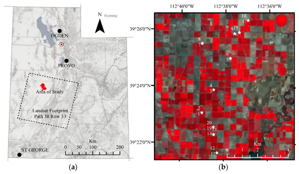
Figure 1.
(a): Landsat Path 38 Row 33 scene footprint (dashed lines) and area of study (black). (b): gap-filled Landsat 7 ETM+ false view (29 May 2012) of the area of study and soil moisture sampling sites (stars) in Central Utah.
3.2. Weather Information
A meteorological station located in the Lower Sevier River Basin (Delta, Utah) provided the weather data for this study. The station is a part of the Community Environmental Monitoring Program (CEMP) in the Desert Research Institute (DRI) network of 29 monitoring stations located in the Western States. The station, located at 39°21’11” N, 112°34’42” W, and 1415 m asl, records hourly solar radiation, air temperature, wind speed, precipitation, and relative humidity. These data are available on the CEMP website [59]. This study included 2012 weather data from January to June.
3.3. Remote Sensing Data
Landsat 7 ETM+ satellite images with a 16-day revisit time were used in this study. These images were already terrain and geometrically processed by the Level 1 Product Generation System at the USGS Center for Earth Resources Observation and Science, EROS [60]. Four cloud-free images, listed in Table 1, were acquired for a period of two months in 2012 covering different crop growth stages for the area of study. The Landsat 7 ETM+ sensor has six bands with 30 m spatial resolution in the shortwave, near-infrared, and mid-infrared portions of the electromagnetic spectrum, while the thermal band has an original spatial resolution of 120 m downscaled to 30m. Due to the 2003 sensor failure in Landsat ETM+ [60], the images for the four Landsat scenes were completed by running a natural neighbor interpolation through the individual bands, as suggested in [61].

Table 1.
Landsat 7 ETM+ images used for this study.
3.4. Surface Soil Moisture Data Collection
During the Landsat overpass dates (Table 1), surface soil moisture measurements were taken at twenty sampling sites within the area of study (indicated by stars in Figure 1). These sites were chosen based on locations in a previous soil moisture network. Soil moisture measurements were made using a Decagon GS3 sensor [62], which measures soil volumetric water content (θ) using a generic calibration that has an accuracy of ±0.03 m3/m3 (±3% θ) [63,64]. A laboratory validation of the GS3 sensor [6] in Central Utah agricultural lands (near the area of study) determined that custom sensor calibration was not required. To account for the spatial footprint of the individual Landsat pixel (30 m by 30 m), several soil moisture measurements were made for each sampling site and posteriorly averaged within the pixel footprint. Table 2 presents details of the crops at each sampling site. The crop types tend to fully cover the surface after the initial development and until the harvest stage. The irrigation method used in the area of study is level basin, in which water covers the entire field during an irrigation event, with no drainage. This type of irrigation is possible because of the laser leveling practice continuously used in the Lower Sevier River Basin.
Table 2.
Installed crops in soil moisture sampling sites.
The measured surface soil moisture ranged from 0.06 to 0.65 m3/m3 (dry soil to water layer) for the four dates. Similar soil moisture ranges for similar crop types in Central Utah are reported by [6] at up to 0.55 m3/m3. Higher soil moisture values represent the basin water in the field due to an irrigation event [62,63]. No distinctive pattern of soil moisture ranges can be identified among crop types or sampling sites (Table 2), due to dissimilar farm management, including irrigation scheduling (on-demand water distribution).
3.5. Potential Surface Soil Moisture Predictors
Surface soil moisture predictors used in this study were selected based on the scientific literature and were included based on the information available for the area of study. The potential soil moisture predictors were then organized in groups by their complexity in estimation/acquisition. Three potential predictor groups were defined: (a) atmospheric variables; (b) Landsat reflectance and vegetation indices; and (c) spatial energy balance (fluxes).
- a)
- Atmospheric Variables: These potential predictors are weather parameters obtained from a typical agricultural weather station and are presented in Table 3. Since precipitation records for the area of study have been historically scarce, rainfall was omitted as a potential predictor.
Table 3. Potential atmospheric predictors considered in this study.
- b)
- Landsat Indices: The Landsat individual surface reflectance, band ratios, vegetation indices, and cap-tasseled images that were calculated for each of the four dates are summarized in Table 4.
Table 4. Potential landsat indices calculated for this study.
- c)
- Evapotranspiration and Energy Balance Components
The METRIC algorithm by [47] was implemented in ERDAS software to process the four Landsat images and obtain spatial estimation of Surface Energy Balance components, actual evapotranspiration (ET24), crop coefficient (ETrF), and water evaporation (Table 5).
Table 5.
METRIC energy balance products used in this study.
3.6. Relevance Vector Machine Calibration
- a)
- The Relevance Vector Machine (RVM)
A 2009 version of the RVM algorithm implemented in Matlab and developed by [65] was used in this study. The kernel functions tested in this study were Gauss, Cauchy, TPS (thin-plate spline), Laplace, Spline, R, Cubic, and Bubble. The RVM algorithm required two parameters to be calibrated: the kernel function type and kernel width. The kernel functions are mathematical equations for likeness comparison of basis functions that originate from predictors themselves [52]. For the second RVM parameter, kernel width (λ), each kernel function requires a single parameter called “width” for adjustment of the kernel amplitude. The kernel width can take any real positive non-zero value. For each tested kernel function, a kernel width range from 0.00001 to 1000 was considered (approximately 700 values).
- b)
- Stratified Cross-Validation
Due to the number of potential soil moisture predictors described in Table 3, Table 4 and Table 5 (47 in total) and the parameters to calibrate the RVM (2 in total), a custom procedure to calibrate the RVM surface soil moisture model was necessary. In addition, because of the limited number of soil moisture ground samples (80 in total) available for this study, it was evident that commonly used hold-out calibration, also known as training and testing subsets [18,66], was not applicable. In similar reported cases, a cross-validation technique (CV) with randomized K-folds (5, 10, 20) has been applied [67]. Nevertheless, traditional randomized K-folds would introduce a bias component in the RVM or any other model. In this study, a modified CV technique is implemented that defines the number of datasets for each K-fold as the number of Landsat scenes used. Thus, the soil moisture samples and potential predictors for a given Landsat date belong to a specific kth-fold. For this study, the number of folds, K, equals four (e.g., May 13 fold#1, May 29 fold #2, etc.); therefore, the CV technique is “stratified” by the collection dates, per se, which avoids bias or randomness effects on the model-performance statistics and ensures repeatability of results.
- c)
- Soil Moisture Predictors Identification
Not all of the 47 potential predictors included in this study were expected to be of equal importance for soil moisture estimation. In addition, it was expected that no prior predictor filtering would be necessary because the forward predictor selection (FPS) procedure [68] implemented in this study would allow the proposed RVM calibration to automatically purge less important predictors. The FPS allows for fast identification of synergistic predictor subsets based on the model performance statistics using the modeling algorithm itself (in this case, the RVM).
All Landsat-derived potential predictors were expected to be correlated to each other to a certain degree at spectral (correlation between predictors) and spatial (neighboring pixels within a predictor) levels because they were derived from the same Landsat reflectance and temperature bands (spectral correlation) and were affected by the optical sensor design (neighboring pixel correlation). While using these predictors would raise issues in customary statistics (e.g., linear regression), Bayesian learning machines, such as the RVM prioritize the synergy effect of predictors and predictor statistical pattern over their statistical or spatial relationships. Nevertheless, Landsat Tasseled Cap products (Brightness, Haze, Greenness, and Wetness) are not expected to be statistically correlated [69]. The inclusion of Tasseled Cap products in this study provided an initial point to assess whether uncorrelated predictors were of higher importance for RVM soil moisture modeling.
The performance statistics obtained from the RVM using the stratified CV and FPS procedure allowed predictor subset candidates (along with kernel function type and width) to be determined. Two statistical parameters, in order of importance, were used in this study: the Root Mean Square Error (RMSE, m3/m3) and the Coefficient of Efficiency or Nash–Sutcliffe Coefficient (η, no units) [70]. These two parameters have been used extensively in hydrological and earth science applications [71]. In addition, because of the number of potential predictors incorporated into the RVM calibration with stratified CV and FPS, there can be cases where two or more different predictor subsets have similar predictive power (similar statistical results). Occam Razor philosophy indicates that, ceteris paribus, simpler models/parameters must have priority over more complex ones. Thus, simpler predictor subsets took priority. This implied that the predictors listed in Table 3 took precedence over those named in Table 4, which in turn took precedence over the ones identified in Table 5.
It is important to mention that the stratified CV was used, along with FPS, solely for identification of suitable predictor subsets along the RVM calibration parameters. The final RVM model selection required an additional step using all collected soil moisture data.
- d)
- Surface Soil Moisture Model Selection
The final surface soil moisture model was selected by comparing the statistical performance of different RVM models generated for potential predictor subset and using the 80 sampling values, called in this document “all (Data)”, as training and testing sets. Again, the performance statistics are RMSE and η. Due to the stratified CV and FPS procedure implemented in this study, model-overfitting issues were minimized. The selected RVM model was then applied to the area of study (Canal B) for the four Landsat dates.
4. Results and Discussion
4.1. Potential Predictors
A sample of the surface soil moisture potential predictors (Atmospheric, Landsat Indices, and Energy Balance Products) used in this study is presented in Table 6 and Figure 2. Figure 3 shows the spatial distribution of the crop coefficient or fractional evapotranspiration (ETrF) for the four Landsat dates. In addition, Figure 4 shows a scatterplot comparison of measured surface soil moisture against ETrF, surface temperature and NDVI.
Table 6.
Daily Weather Information for Landsat overpass dates.
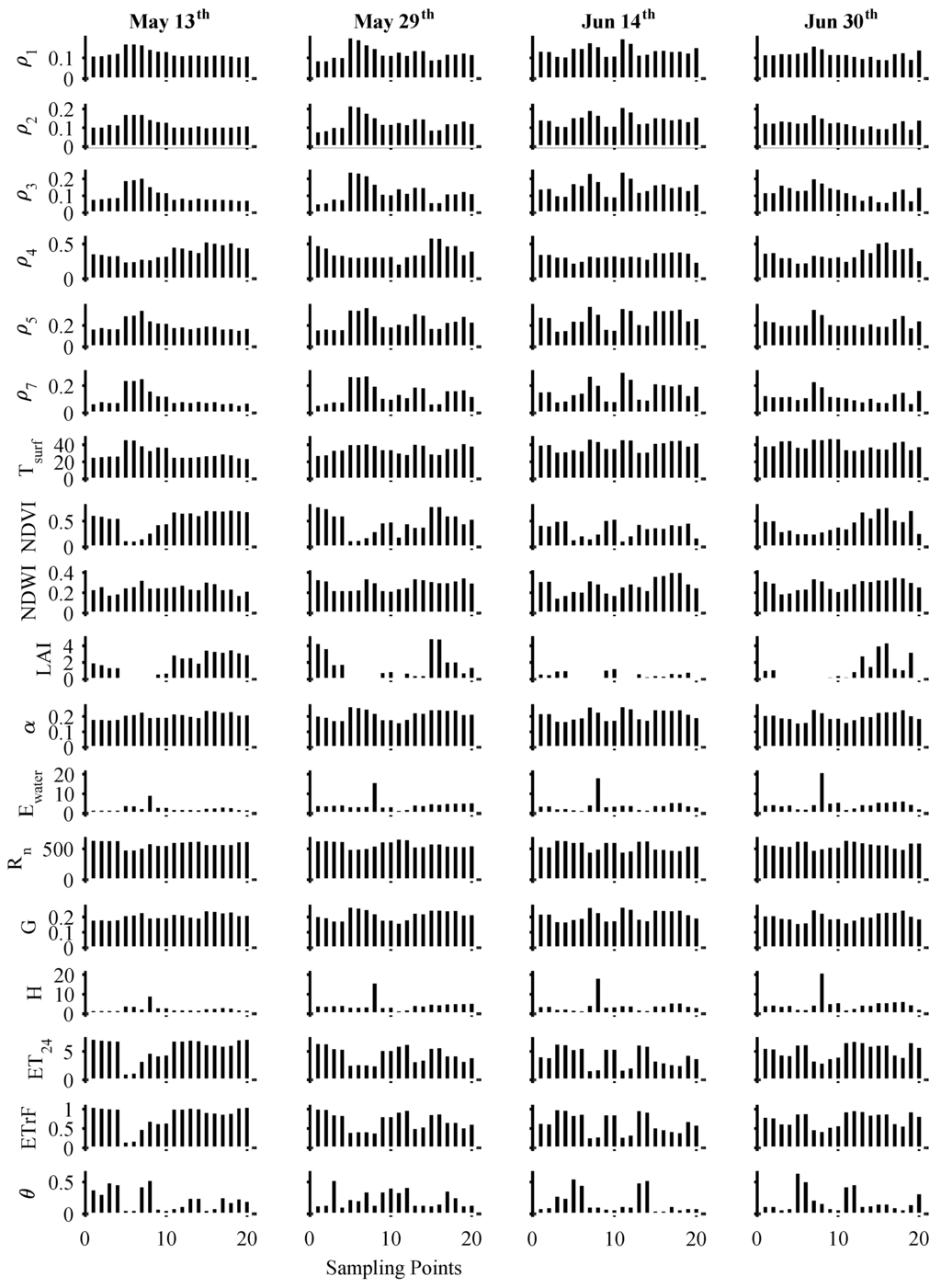
Figure 2.
Measured surface soil moisture (bottom row) and corresponding Landsat indices and metric energy balance products (upper rows) for the four Landsat overpass dates considered in the study.
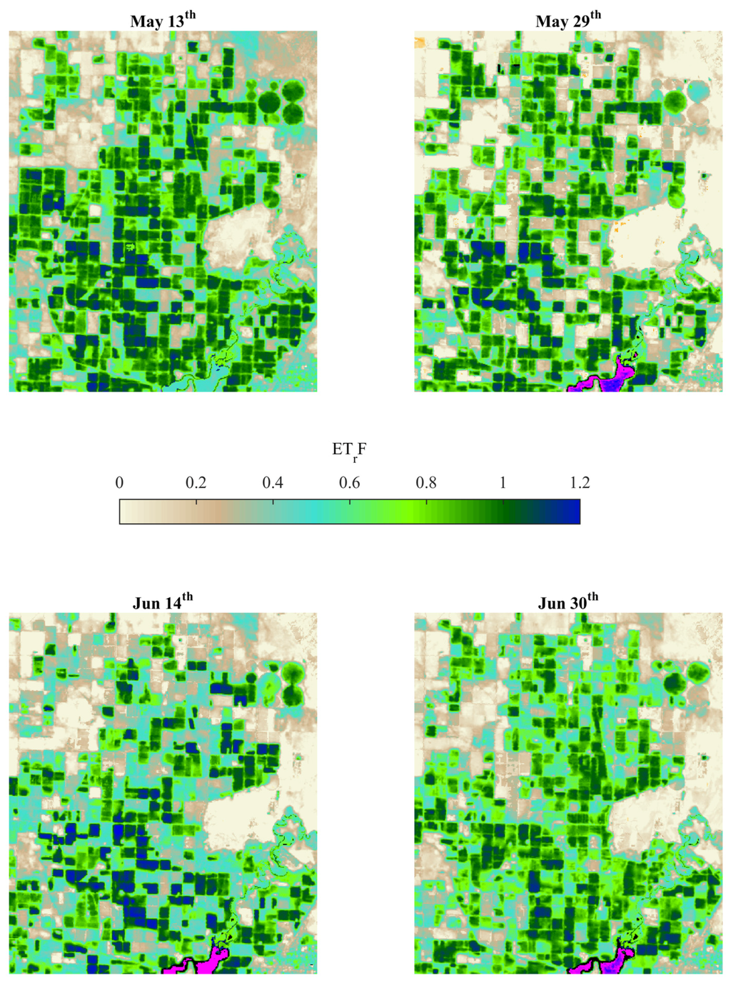
Figure 3.
ETrF maps using METRIC model and Landsat 7 ETM+ images for the area of study. Note the absence of gaps in the maps due to the use of the natural neighboring interpolation technique on the original DN bands.
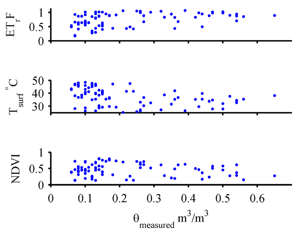
Figure 4.
Measured surface soil moisture comparison with METRIC fractional evapotranspiration (top), Landsat surface temperature (mid), and NDVI (bottom) values for the four dates considered in this study.
The information presented in Figure 2, Figure 4, and Table 6 indicate that measured surface soil moisture did not have a linear relationship with any of the potential predictors included in this study. Figure 4 also indicates that there is no identifiable trend between Landsat fractional evapotranspiration (ETrF), surface temperature, nor NDVI with measured surface soil moisture values.
4.2. Model Development
The stratified CV along with FPS used in this study was implemented at the High Performance Computing facility at Utah State University. Due to the large number of computational runs for each individual kernel type, only a selection of the best performance runs is shown in Table 7. Figure 5 presents a detailed view of the statistical performance during FPS using the “Bubble” kernel and all available samples (all (Data)).
Table 7.
RVM statistics for best soil moisture models using each kernel type.
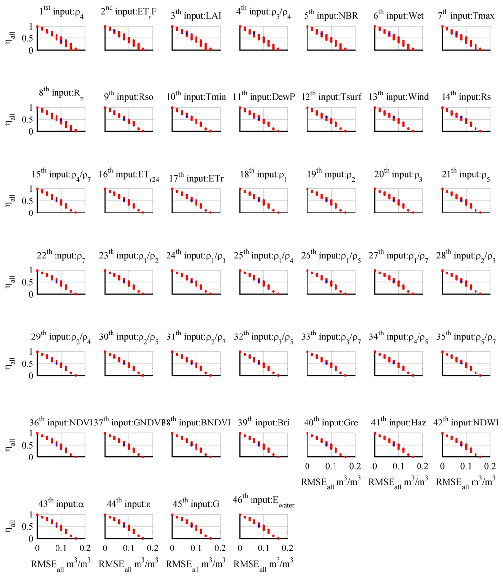
Figure 5.
Example of RMSE and η values for fourty-six FPS iterations using RVM with a bubble kernel function. Subplot title indicated variable selected for the i-th FPS iteration. Red dots are statistical result values for considered kernel width values using all (Data). Blue dots are all (Data) statistical results of selected stratified CV inputs for each iteration.
Due to the stratified CV, differences among results for all (Data) vs. CV statistics are small (Table 7). Nevertheless, when comparing models using CV and all (Data) results, statistics from the CV should be considered as true descriptors of the RVM model performance.
Table 7 also indicates that, from among the kernel types tested, the RVM model using the “Bubble” kernel best identifies a relationship between four potential predictors (NIR band, ρ4; fractional evapotranspiration, ETrF; leaf area index, LAI; and the band ratio Red/NIR, ρ3/ρ4) and surface soil moisture. The results from the other RVM models, with different kernel types, showed different selections of predictors using the forward predictor selection procedure but with poorer statistical performance.
Figure 5 provides a detailed description of the RVM model performance with the bubble kernel when using the same information for training and testing purposes (all (Data) statistical results). Due to the evaluated kernel width range, some statistical results (red dots) will have a perfect score or overfitting conditions (RSME ≈ 0 m3/m3, η ≈ 1), which have a poor statistical performance on the CV results. In the same figure, for each forward predictor selection iteration, the best RVM models based on stratified CV results (blue dots) do not suffer from these overfitting conditions.
The selection of the best RVM model for each kernel type (presented in Table 7) was performed by assessment of the statistical performance in the stratified crossvalidation and all (Data) runs (same as Table 7), statistical plots (same as Figure 6), and spatial mapping of the results (e.g., Figure 7) for each of the forty-six iterations. Thus, an RVM model with the bubble kernel and two inputs (ρ4 and ETrF) was rejected as the best model despite having all (Data) statistics of RMSE = 0.02 and η = 0.8, as shown in Figure 5 because the spatial soil moisture map developed for this specific model exhibited overfitting characteristics (constant soil moisture values) across the maps.
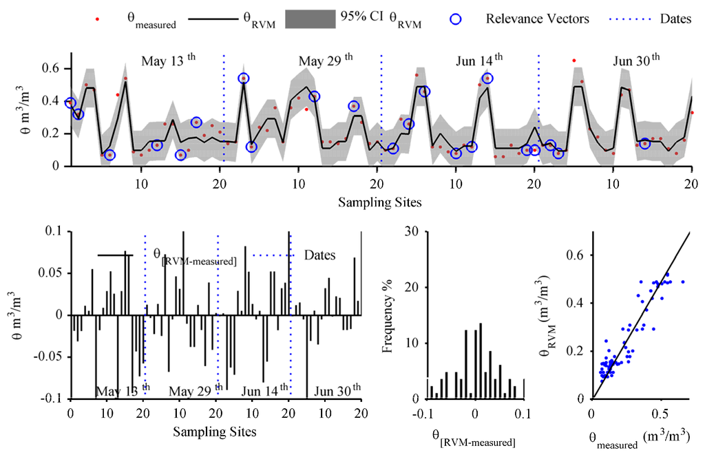
Figure 6.
Performance of the soil moisture RVM model, including the 95% confidence interval (CI) using the bubble kernel using all available data: (top) measured vs. RVM soil moisture values, (lower left) residual distribution, (lower center), residual histogram and (lower right) 1:1 measured vs. RVM surface soil moisture plot.
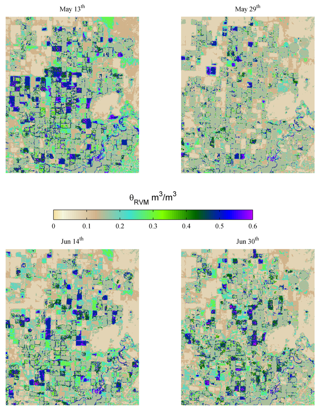
Figure 7.
Spatial Estimation of Surface Soil Moisture for the four Landsat 7 ETM+ dates using the RVM model with the bubble kernelkernel. Note: Soil moisture values higher than 0.5 m3/m3 indicate fields under irrigation.
The predictor subset selected by the RVM model with the bubble kernelkernel (Table 7) indicated the synergy and need of these predictors to estimate surface soil moisture. The NIR band is a relative indicator of vegetation variability; ETrF indicates the water consumption ratio from the root zone; the red/NIR band ratio, also known as the simple ratio or Ratio Vegetation Index [72], allows for relative estimation of soil moisture from dry to moist conditions; and finally, LAI is a direct indicator of crop biomass per pixel. These four predictors contain the necessary spatial pattern for the RVM algorithm to estimate surface soil moisture for the crop types and status present in Central Utah (full cover crops). In addition, the inclusion of more than one predictor in the RVM also indicates that the spatial pattern of the surface soil moisture does not follow the spatial pattern of a single predictor (e.g., ETrF or NDVI).
Figure 6 and Figure 7 show the statistical and spatial behavior of the selected RVM model (Bubble Kernel, four predictors). In Figure 6, the adequate correlation of the RVM model to the measured surface soil moisture is evident: 1:1 relationship between measured and estimated values, normal (or Gaussian) distribution of the model residuals, and random pattern in the occurrence of residuals. In Figure 7 the resulting spatial soil moisture on the surface can be seen for the four Landsat dates used in this study. In general terms, the soil moisture values within each field tend to be alike because of the irrigation type (gravity flooding of laser-leveled fields) employed by all farmers in the area of study. Thus, high soil moisture values will occurs in fields recently irrigated and low values in fields where the last irrigation event was not recent. Within fields, the RVM model seems to be able to recognize small differences at the pixel level, which can be an indication of soil characteristics (texture, structure, type), although these differences can fall within the accuracy of the RVM model (CV RMSE = 0.10 m3/m3). Outside agricultural fields, it seems that the RVM is able to infer surface soil moisture in fallow or non-cultivated areas, although no ground information is available to confirm this. The developed RVM model does not recognize open water surfaces, given that no information about these locations (in the southern portion of the area of study) was provided during the calibration process. Finally, the RVM seems to have limited performance in locations with mixed pixel information (fields with canals or houses), which creates an identifiable perimeter for most fields. This is because Landsat 30-m/pixel resolution does not allow for a direct discrimination of non-agricultural pixels. A spatial filter based on the National Land Cover Database NLCD [73] and used by the METRIC ET algorithm can help to discriminate these mixed pixels in Landsat images and the soil moisture maps of this study.
As with any proposed methodology, uncertainty sources and identified limitations in this study must be identified. The uncertainty sources in this study were the various error sources that affect collected soil moisture and weather data as explained by [74]. For Landsat, major uncertainty sources are the occurrence of transparent cirrus clouds/haze, radiometric calibration, and optical distortion on pixel reflectance as described by [75,76]. Additionally, Landsat’s camera quality degradation can also affect the remotely sensed information [77,78]. In addition, Landsat ETM+ images presented gaps, which were filled for this study. METRIC algorithm, despite its extensive use in research, may require validation to determine its actual local accuracy [79]. Finally, in the presented study, the selected RVM model is not expected to perform adequately on non-agricultural or mixed pixel areas such as roads, urban areas, wetlands, and open water. These uncertainty sources must be taken into account when using the presented methodology.
5. Conclusions
This study presented a methodology to estimate surface soil moisture from atmospheric variables, Landsat vegetation indices, and energy balance products. A relevance vector machine, RVM, along with stratified crossvalidation and forward predictor selection, was used to build the surface soil moisture model for the irrigated lands located in the Central Utah area of study. The methodology presented here allowed a fast discrimination from 47 potential predictors cited in scientific literature with a calibration process that required statistical and visual (spatial) validation to determine the best predictor subset that strongly relates to surface soil moisture.
The results of this study indicate that a single spatial parameter (e.g., ETrF or NDVI) cannot describe the surface soil moisture behavior in temporal nor spatial scales. From 47 selected predictors included in this study, the proposed methodology for estimation of surface soil moisture identified four: (1) spatial vegetation variability (NIR band); (2) evapotranspiration rates (ETrF); (3) relative soil moisture variation (Red/NIR ratio); and (4) biomass estimation (LAI). These predictors provided the best spatial estimation of surface soil moisture in the agricultural lands at the Central Utah site, from dry soil to irrigated conditions, regardless of the canopy development (from bare soil to full development).
The methodology presented here can be used to derive surface soil moisture for any other agricultural site that has measured soil moisture information, regardless of the crops that are grown. For different crop distributions and irrigation practices than those employed in Central Utah (full cover crops, alfalfa, corn, small grains, and basin irrigation, respectively), the proposed methodology may select additional, or even different, predictors than the ones selected by this study. This characteristic of the proposed methodology can be very useful for specialty crops (orchards, high value crops, herbs, etc.), where different satellite or aerial platforms than Landsat are available (e.g., manned aircraft, commercial satellites). In addition, the presented methodology may have application for natural environments, if measured soil moisture information is available, as can be inferred from the RVM results of the soil moisture model for fallow areas in the area of study. Therefore, this methodology can improve understanding of soil-moisture-related processes in other places with different land and crop types.
This study relied on standard procedures for Landsat vegetation indices and surface energy balance products as proposed in scientific literature, with their related accuracies and uncertainties. Nevertheless, embedded uncertainty in the spatial information is not expected to translate into the proposed soil moisture model using the RVM algorithm due to the nature of the RVM statistical modeling (as opposed to physical modeling). Nevertheless, it is advisable to apply quality control procedures for the validation of spatial information (Landsat for this study), especially for gap-filling, spatial evapotranspiration, and energy balance component products.
In remote sensing applications, autocorrelation in the spatial data (among bands and neighboring pixels) is expected. This is due to optics design, selected spectral bands, and smoothing and downsampling applications (e.g., NASA standard cubic convolution filter applied to all Landsat records, especially on the thermal band), among others. In physical-based models (e.g., land surface models) this autocorrelation characteristic could have a high impact on modeled results, but in the RVM learning machine model used in this study, the statistical behavior for each of the potential predictors is the modeled characteristic related to measured surface soil moisture. Nevertheless, within the potential predictors included in this study, four Landsat uncorrelated inputs were evaluated (Brightness, Haze, Greenness, and Wetness) to initially determine if these predictors were of higher importance for soil moisture modeling. The obtained results (predictors selected by the RVM algorithm) indicated that they were not.
Future work could include estimating soil moisture at deeper levels and soil water content (on which this study can play an important role), along with forecasting spatial ET and soil water content for integration in irrigation water balance operational schemes at field and command areas using Landsat and MODIS Terra satellite platforms. In addition, procedures to quantify and minimize the impact of data and model uncertainty sources in results need to be developed, such as initial USGS efforts for standard Landsat surface level reflectance and temperature products.
Acknowledgments
This project was supported by the Utah Water Research Laboratory at Utah State University (Mineral Lease Funds WR-2188). Historical and real-time hourly weather data for the Lower Sevier River Basin were graciously provided by the Community Environmental Monitoring Program (Nevada). The authors also thank Roger Hansen at the Provo, Utah, office of the U.S. Bureau of Reclamation; James Walker, the Lower Sevier Basin Commissioner; and the Sevier River Water Users Association for their continued assistance and support in this research.Appreciation goes to Carri Richards for her timely help in editing the paper. Landsat data are distributed by the Land Processes Distributed Active Archive Center (LP DAAC), located at USGS/EROS, Sioux Falls, SD. http://lpdaac.usgs.gov. Computer, storage, and other resources from the High Performance Computing—Division of Research Computing in the Office of Research and Graduate Studies at Utah State University are gratefully acknowledged.
Author Contributions
Mac McKee, Roula Bachour, and Alfonso Torres-Rua conceived and designed the study; Andres M. Ticlavilca and Roula Bachour performed the data collection; Roula Bachour and Alfonso Torres-Rua analyzed the data; Andres Ticlavilca, Mac McKee, and Roula Bachour performed the draft manuscript review; Alfonso Torres-Rua wrote the present manuscript.
Conflicts of Interest
The authors declare no conflict of interest.
References
- Walker, W.R. Lessons for the Last Half Century of Irrigation Engineering Research—Where to Now? In IV Congreso Nacional y III Congreso Iberoamericano de Riego y Drenaje; La Molina National Agrarian University: Lima, Peru, 2011. [Google Scholar]
- Anderson, M.C.; Allen, R.G.; Morse, A.; Kustas, W.P. Use of Landsat thermal imagery in monitoring evapotranspiration and managing water resources. Remote Sens. Environ. 2012, 122, 50–65. [Google Scholar] [CrossRef]
- Allen, R.; Irmak, A.; Trezza, R.; Hendrickx, J.M.H.; Bastiaanssen, W.; Kjaersgaard, J. Satellite-based ET estimation in agriculture using SEBAL and METRIC. Hydrol. Process. 2011, 25, 4011–4027. [Google Scholar] [CrossRef]
- Kogan, F.N.F. Operational space technology for global vegetation assessment. Bull. Am. Meteorol. Soc. 2001, 82, 1949–1964. [Google Scholar] [CrossRef]
- National Geospatial Advisory Committee (NGAC). The Value Proposition for Ten Landsat Applications; NGAC: Washington, DC, USA, 2012; pp. 1–6. [Google Scholar]
- Hassan-Esfahani, L.; Torres-Rua, A.F.; Ticlavilca, A.M.; Jensen, A.; McKee, M. Topsoil moisture estimation for precision agriculture using unmmaned aerial vehicle multispectral imagery. In Proceedings of the 2014 IEEE Geoscience and Remote Sensing Symposium, Quebec, QC, Canada, 13–18 July 2014; pp. 3263–3266.
- Petropoulos, G. Remote Sensing of Energy Fluxes and Soil Moisture Content; CRC Press: Boca Raton, FL, USA, 2013. [Google Scholar]
- Hassan-Esfahani, L.; Torres-Rua, A.; McKee, M. Assessment of optimal irrigation water allocation for pressurized irrigation system using water balance approach, learning machines, and remotely sensed data. Agric. Water Manag. 2015, 153, 42–50. [Google Scholar] [CrossRef]
- Islam, S.; Engman, T.; Kivelson, M.; Islam, S.; Engman, T. Why bother for 0.0001% of Earth's water: Challenges for soil moisture research. Eos Trans. Am. Geophys. Union 1996, 77, 420. [Google Scholar] [CrossRef]
- Small, E.; Kurc, S. The Influence of Soil Moisture on the Surface Energy Balance in Semiarid Environments; Water Resources Research Institute: Las Cruces, NM, USA, 2001. [Google Scholar]
- Liu, Y.Y.; Parinussa, R.M.; Dorigo, W.A.; de Jeu, R.A.M.; Wagner, W.; van Dijk, A.I.J.M.; McCabe, M.F.; Evans, J.P. Developing an improved soil moisture dataset by blending passive and active microwave satellite-based retrievals. Hydrol. Earth Syst. Sci. 2011, 15, 425–436. [Google Scholar] [CrossRef]
- Yin, J.; Zhan, X.; Zheng, Y.; Liu, J.; Fang, L.; Hain, C.R. Enhancing Model Skill by Assimilating SMOPS Blended Soil Moisture Product into Noah Land Surface Model. J. Hydrometeorol. 2015, 16, 917–931. [Google Scholar] [CrossRef]
- Gassman, P.; Williams, J.; Benson, V.; Izaurralde, R.C.; Hauck, L.M.; Jones, C.A.; Atwood, J.D.; Kiniry, J.R.; Flowers, J.D. Historical Development and Applications of the EPIC and APEX Models; Center for Agricultural and Rural Development, Iowa State University: Ames, IA, USA, 2005. [Google Scholar]
- Andris, C.; Cowen, D.; Wittenbach, J. Support Vector Machine for Spatial Variation. Trans. GIS 2013, 17, 41–61. [Google Scholar] [CrossRef]
- Bachour, R.; Walker, W.R.; Ticlavilca, A.M.; McKee, M.; Maslova, I. Estimation of Spatially Distributed Evapotranspiration Using Remote Sensing and a Relevance Vector Machine. J. Irrig. Drain. Eng. 2014, 140, 04014029. [Google Scholar] [CrossRef]
- Batt, H.A.; Stevens, D.K. How to Utilize Relevance Vectors to Collect Required Data for Modeling Water Quality Constituents and Fine Sediment in Natural Systems: Case Study on Mud Lake, Idaho. J. Environ. Eng. 2014, 140, 06014003. [Google Scholar] [CrossRef]
- Kaheil, Y.H.; Gill, M.K.; McKee, M.; Bastidas, L.A.; Rosero, E. Downscaling and Assimilation of Surface Soil Moisture Using Ground Truth Measurements. IEEE Trans. Geosci. Remote Sens. 2008, 46, 1375–1384. [Google Scholar] [CrossRef]
- Gill, M.K.; Kemblowski, M.W.; McKee, M.; Gill, M.K.; Kemblowski, M.W.; McKee, M. Soil Moisture Data Assimilation Using Support Vector Machines and Ensemble Kalman Filter. J. Am. Water Resour. Assoc. 2007, 43, 1004–1015. [Google Scholar] [CrossRef]
- Khader, A.I.; McKee, M. Use of a relevance vector machine for groundwater quality monitoring network design under uncertainty. Environ. Model. Softw. 2014, 57, 115–126. [Google Scholar] [CrossRef]
- Zaman, B.; McKee, M. Spatio-temporal Prediction of Root Zone Soil Moisture Using Multivariate Relevance Vector Machines. Open J. Mod. Hydrol. 2014, 4, 80–90. [Google Scholar] [CrossRef]
- Zaman, B.; McKee, M.; Neale, C.M.U. Fusion of remotely sensed data for soil moisture estimation using relevance vector and support vector machines. Int. J. Remote Sens. 2012, 33, 6516–6552. [Google Scholar] [CrossRef]
- Margulis, S.A.; McLaughlin, D.; Entekhabi, D.; Dunne, S. Land data assimilation and estimation of soil moisture using measurements from the Southern Great Plains 1997 Field Experiment. Water Resour. Res. 2002, 38, 35:1–35:18. [Google Scholar] [CrossRef]
- Sànchez-Marrè, M.; Béjar, J.; Comas, J.; Brocca, L.; Melone, F.; Moramarco, T. Soil Moisture Monitoring at Different Scales for Rainfall-Runoff Modelling. In Proceedings of International Congress on Environmental Modelling and Software (iEMSs 2008), Barcelona, Spain, 7–10 July 2008; Volume 1, pp. 407–414.
- Njoku, E.G.; Wilson, W.J.; Yueh, S.H.; Dinardo, S.J.; Li, F.K.; Jackson, T.J.; Lakshmi, V.; Bolten, J. Observations of soil moisture using a passive and active low-frequency microwave airborne sensor during SGP99. IEEE Trans. Geosci. Remote Sens. 2002, 40, 2659–2673. [Google Scholar] [CrossRef]
- Sabater, J.M.; Jarlan, L.; Calvet, J.-C.; Bouyssel, F.; De Rosnay, P. From Near-Surface to Root-Zone Soil Moisture Using Different Assimilation Techniques. J. Hydrometeorol. 2007, 8, 194–206. [Google Scholar] [CrossRef]
- Moran, M.S.; Peters-Lidard, C.D.; Watts, J.M.; McElroy, S. Estimating soil moisture at the watershed scale with satellite-based radar and land surface models. Can. J. Remote Sens. 2004, 30, 805–826. [Google Scholar] [CrossRef]
- Entekhabi, D.; Njoku, E.G.; O’Neill, P.E.; Kellogg, K.H.; Crow, W.T.; Edelstein, W.N.; Entin, J.K.; Goodman, S.D.; Jackson, T.J.; Johnson, J.; et al. The soil moisture active passive (SMAP) mission. Proc. IEEE 2010, 98, 704–716. [Google Scholar] [CrossRef]
- Piles, M.; Entekhabi, D.; Camps, A. A Change Detection Algorithm for Retrieving High-Resolution Soil Moisture From SMAP Radar and Radiometer Observations. IEEE Trans. Geosci. Remote Sens. 2009, 47, 4125–4131. [Google Scholar] [CrossRef]
- Jackson, R.D.; Idso, S.B.; Reginato, R.J.; Pinter, P.J. Canopy temperature as a crop water stress indicator. Water Resour. Res. 1981, 17, 1133–1138. [Google Scholar] [CrossRef]
- Wetzel, P.; Atlas, D.; Woodward, R.; Werzel, P.; Atlas, D.; Woodward, R. Determining soil moisture from geosynchronous satellite infrared data. J. Climatol. Appl. Meteorol. 1984, 23, 375–391. [Google Scholar] [CrossRef]
- Ahmad, M.-D.; Bastiaanssen, W.G.M. Retrieving Soil Moisture Storage in the Unsaturated Zone Using Satellite Imagery and Bi-Annual Phreatic Surface Fluctuations. Irrig. Drain. Syst. 2003, 17, 141–161. [Google Scholar] [CrossRef]
- Hendrickx, J.M.H.; Hong, S.; Friesen, J.; Compaore, H.; van de Giesen, N.C.; Rodgers, C.; Vlek, P.L.G. Mapping Energy Balance Fluxes and Root Zone Soil Moisture in the White Volta Basin using Optical Imagery. Proc. SPIE 2006, 6239, 62390Q:1–62390Q:12. [Google Scholar]
- Scott, C.A.; Bastiaanssen, W.G.M.; Ahmad, M.-D. Mapping Root Zone Soil Moisture Using Remotely Sensed Optical Imagery. J. Irrig. Drain. Eng. 2003, 129, 326–335. [Google Scholar] [CrossRef]
- Levitt, D.G.; Simpson, J.R.; Huete, A.R. Estimates of surface soil water content using linear combinations of spectral wavebands. Theor. Appl. Climatol. 1990, 42, 245–252. [Google Scholar] [CrossRef]
- Musick, H.B.; Pelletier, R.E. Response of some Thematic Mapper band ratios to variation in soil water content. Photogramm. Eng. Remote Sens. 1986, 52, 1661–1668. [Google Scholar]
- Miller, J.D.; Yool, S.R. Mapping forest post-fire canopy consumption in several overstory types using multi-temporal Landsat TM and ETM data. Remote Sens. Environ. 2002, 82, 481–496. [Google Scholar] [CrossRef]
- Idso, S.B.; Jackson, R.D.; Reginato, R.J.; Kimball, B.A.; Nakayama, F.S. The Dependence of Bare Soil Albedo on Soil Water Content. J. Appl. Meteorol. 1975, 14, 109–113. [Google Scholar] [CrossRef]
- Carlson, T.N.; Dodd, J.K.; Benjamin, S.G.; Cooper, J.N. Satellite Estimation of the Surface Energy Balance, Moisture Availability and Thermal Inertia. J. Appl. Meteorol. 1981, 20, 67–87. [Google Scholar] [CrossRef]
- Li, J.; Islam, S. Estimation of root zone soil moisture and surface fluxes partitioning using near surface soil moisture measurements. J. Hydrol. 2002, 259, 1–14. [Google Scholar] [CrossRef]
- Saxton, K.E.; Johnson, H.P.; Shaw, R.H. Modeling evapotranspiration and soil moisture. Trans. ASAE 1974, 17, 673–677. [Google Scholar] [CrossRef]
- Saxton, K.; Willey, P. The SPAW Model for Agricultural Field and Pond Hydrologic Simulation. In Watershed Models, 1st ed.; CRC Press: Boca Raton, FL, USA, 2005; pp. 400–435. [Google Scholar]
- Holtan, H.N.; Lopez, N.C. USDAHL-70 Model of Watershed Hydrology; Agricultural Research Service, U.S. Department of Agriculture: Washington, DC, USA, 1971. [Google Scholar]
- Holtan, H.N. USDAHL-74 Revised Model of Watershed Hydrology a United States Contribution to the International Hydrological Decade; Agricultural Research Service, U.S. Department of Agriculture: Washington, DC, USA, 1975. [Google Scholar]
- Peck, E.L. Catchment Modeling with the United States National Weather Service River Forecast System; NOAA: Washington, DC, USA, 1976. [Google Scholar]
- Shuttleworth, W.J. Terrestrial Hydrometeorology, 1st ed.; John Wiley & Sons, Ltd.: Chichester, UK, 2012. [Google Scholar]
- Das, N.N.; Mohanty, B.P. Root Zone Soil Moisture Assessment Using Remote Sensing and Vadose Zone Modeling. Vadose Zo. J. 2006, 5, 296. [Google Scholar] [CrossRef]
- Allen, R.G.; Tasumi, M.; Morse, A.; Trezza, R.; Wright, J.L.; Bastiaanssen, W.; Kramber, W.; Lorite, I.; Robison, C.W. Satellite-Based Energy Balance for Mapping Evapotranspiration with Internalized Calibration (METRIC)—Model. J. Irrig. Drain. Eng. 2007, 133, 395–406. [Google Scholar] [CrossRef]
- Liang, S. Quantitative Remote Sensing of Land Surfaces; Wiley-Interscience: Hoboken, NJ, USA, 2004. [Google Scholar]
- Allen, R.G.; Pereira, L.S.; Raes, D.; Smith, M. Crop Evapotranspiration: Guidelines for Computing Crop Requirements; FAO Irrigation and Drainage Paper 56; Food and Agriculture Organization of the United Nations (FAO): Rome, Italy, 1998. [Google Scholar]
- Allen, R.G.; Tasumi, M.; Morse, A.; Trezza, R.; Wright, J.L.; Bastiaanssen, W.; Kramber, W.; Lorite, I.; Robison, C.W. Satellite-Based Energy Balance for Mapping Evapotranspiration with Internalized Calibration (METRIC)—Applications. J. Irrig. Drain. Eng. 2007, 133, 395–406. [Google Scholar] [CrossRef]
- Tasumi, M. Progress in Operational Estimation of Regional Evapotranspiration Using Satellite Imagery; University of Idaho: Moscow, ID, USA, 2003. [Google Scholar]
- Tipping, M.E. The Relevance Vector Machine. Adv. Neural Inf. Process. Syst. 2000, 12, 652–658. [Google Scholar]
- Tipping, M.E.; Faul, A. Fast marginal likelihood maximisation for sparse Bayesian models. In Ninth International Workshop on Artificial Intelligence and Statistics; AISTATSS: Key West, FL, USA, 2003. [Google Scholar]
- Al-Arab, M.; Torres-Rua, A.; Ticlavilca, A.; Jensen, A.; McKee, M. Use of high-resolution multispectral imagery from an unmanned aerial vehicle in precision agriculture. In 2013 IEEE International Geoscience and Remote Sensing Symposium—IGARSS, Melbourne, VIC, Australia, 21–26 July 2013; pp. 2852–2855.
- Elarab, M.; Ticlavilca, A.M.; Torres-Rua, A.F.; Maslova, I.; McKee, M. Estimating chlorophyll with thermal and broadband multispectral high resolution imagery from an unmanned aerial system using relevance vector machines for precision agriculture. Int. J. Appl. Earth Obs. Geoinf. 2015, 43, 32–42. [Google Scholar] [CrossRef]
- Tipping, M.E. Sparse Bayesian Learning and the Relevance Vector Machine. J. Mach. Learn. Res. 2000, 1, 211–244. [Google Scholar]
- Fletcher, T. Relevance Vector Machines Explained; University College London: London, UK, 2010. [Google Scholar]
- Tipping, M.E.; Faul, A. Analysis of sparse Bayesian learning. Adv. Neural Inf. Process. Syst. 2002, 14, 383–389. [Google Scholar]
- DRI. Community Environmental Monitoring Program|CEMP—DOE. 2014. Available online: cemp.dri.edu (accessed on 1 January 2012).
- LPSO. Landsat Project Science Office—Landsat 7 Science Data Users Handbook; NASA: Greenbelt, MD, USA, 2008. [Google Scholar]
- Allen, R.; Trezza, A.R.; Tasumi, M.; Kjaersgaard, J. Metric Application Manual for Landsat Satellite Imagery; University of Idaho: Kimberly, ID, USA, 2012. [Google Scholar]
- Decagon Devices Inc. GS3 Operator’s Manual; Decagon Devices Inc.: Pullman, WA, USA, 2014. [Google Scholar]
- Decagon Devices Inc. GS3 User Manual; Decagon Devices Inc.: Pullman, WA, USA, 2012. [Google Scholar]
- Cobos, D.R.; Chambers, C.; Clarke, T.R.; Chambers, C. Calibrating ECH2O Soil Moisture Sensors; Decagon Devices Inc.: Pullman, WA, USA, 2010. [Google Scholar]
- Vector Anomaly Ltd. Vector Anomaly: Sparsebayes Software. 2009. Available online: http://www.vectoranomaly.com/downloads/downloads.htm (accessed on 20 November 2011).
- Arlot, S.; Celisse, A. A survey of cross-validation procedures for model selection. Stat. Surv. 2010, 4, 40–79. [Google Scholar] [CrossRef]
- Ruß, G. From Spatial Data Mining in Precision Agriculture to Environmental Data Mining. In Computational Intelligence in Intelligent Data Analysis; Springer Berlin Heidelberg: Berlin, Germany, 2013; pp. 263–273. [Google Scholar]
- Guyon, I.; Elisseeff, A. An introduction to variable and feature selection. J. Mach. Learn. Res. 2003, 3, 1157–1182. [Google Scholar]
- Crist, E.P.; Cicone, R.C. A Physically-Based Transformation of Thematic Mapper Data—The TM Tasseled Cap. IEEE Trans. Geosci. Remote Sens. 1984, 3, 256–263. [Google Scholar] [CrossRef]
- Nash, J.; Sutcliffe, J. River flow forecasting through conceptual models part I—A discussion of principles. J. Hydrol. 1970, 10, 282–290. [Google Scholar] [CrossRef]
- Moriasi, D.; Arnold, J.; van Liew, M. Model evaluation guidelines for systematic quantification of accuracy in watershed simulations. Trans. ASABE 2007, 50, 885–900. [Google Scholar] [CrossRef]
- Tucker, C.J. Red and photographic infrared linear combinations for monitoring vegetation. Remote Sens. Environ. 1979, 8, 127–150. [Google Scholar] [CrossRef]
- Homer, C.; Huang, C.; Yang, L.; Wylie, B.; Coan, M. Development of a 2001 national land-cover database for the United States. Photogramm. Eng. Remote Sens. 2004, 70, 829–840. [Google Scholar] [CrossRef]
- Torres-Rua, A.F.; Ticlavilca, A.M.; Walker, W.R.; McKee, M. Machine Learning Approaches for Error Correction of Hydraulic Simulation Models for Canal Flow Schemes. J. Irrig. Drain. Eng. 2012, 138, 999–1010. [Google Scholar] [CrossRef]
- Huang, C.; Townshend, J.R.G.; Liang, S.; Kalluri, S.N.V.; DeFries, R.S. Impact of sensor’s point spread function on land cover characterization: Assessment and deconvolution. Remote Sens. Environ. 2002, 80, 203–212. [Google Scholar] [CrossRef]
- Wenny, B.; Helder, D.; Hong, J.; Leigh, L.; Thome, K.; Reuter, D. Pre- and Post-Launch Spatial Quality of the Landsat 8 Thermal Infrared Sensor. Remote Sens. 2015, 7, 1962–1980. [Google Scholar] [CrossRef]
- Markham, B.L.; Storey, J.C.; Williams, D.L.; Irons, J.R. Landsat sensor performance: history and current status. IEEE Trans. Geosci. Remote Sens. 2004, 42, 2691–2694. [Google Scholar] [CrossRef]
- Tasumi, M.; Trezza, R.; Allen, R.G.; Wright, J.L. Operational aspects of satellite-based energy balance models for irrigated crops in the semi-arid U.S. Irrig. Drain. Syst. 2005, 19, 355–376. [Google Scholar] [CrossRef]
- Morton, C.G.; Huntington, J.L.; Pohll, G.M.; Allen, R.G.; McGwire, K.C.; Bassett, S.D. Assessing Calibration Uncertainty and Automation for Estimating Evapotranspiration from Agricultural Areas Using METRIC. J. Am. Water Resour. Assoc. 2013, 49, 549–562. [Google Scholar] [CrossRef]
© 2016 by the authors; licensee MDPI, Basel, Switzerland. This article is an open access article distributed under the terms and conditions of the Creative Commons Attribution (CC-BY) license (http://creativecommons.org/licenses/by/4.0/).