Simulation of Summer Hourly Stream Flow by Applying TOPMODEL and Two Routing Algorithms to the Sparsely Gauged Lhasa River Basin in China

Abstract

This paper develops a new routing algorithm for improving simulation capacity of physically-based hydrological models applied to sparsely-gauged river basins. The study area is the Lhasa River basin, a large plateau basin with an area of 26,225 km² in southwest China. In the basin, observations from three hydrological stations are available, and the observed hourly rainfall and summer stream flow data (12 June to 30 September) for the period of 1998–2000 obtained from the three stations were used. TOPMODEL, with its original routing algorithm, which is a distance-related delay function, was applied to the Lhasa River basin. To improve the routing algorithm using a unit hydrograph function and a linear reservoir method, this study proposed a new algorithm; the results revealed that the new algorithm improved the simulation of the variation of hourly stream flow. In addition, to evaluate the influence of rainfall spatial variation on runoff generation, observed rainfall series from the three gauges were used to simulate runoff individually, and it was found that there are significant differences among the three simulated hourly stream flow series.

1. Introduction

TOPographic Model (TOPMODEL) is a rainfall-runoff model developed using the simple theory of hydrological similarity, with the topographic index designed to represent hydrological similarity [1,2,3,4,5]. The original routing algorithm for TOPMODEL simulates the stream flow by transferring the runoff to the basin outlet using a time-delay function. Table 1 presents some example applications of TOPMODEL to different river basins around the world. These applications generally indicate that TOPMODEL has mostly been applied to small river basins or data-rich river basins. In regards to sparsely-gauged large river basins, the exploration of the available routing algorithms for stream flow simulation is particularly lacking. To address this issue, the present study analyses the simulation capacity of TOPMODEL in a sparsely-gauged river basin. The Lhasa River basin in southwestern China is considered as the study area, and summer hourly stream flow in the basin is simulated. A new routing algorithm for TOPMODEL is proposed, and the results from the original and the new routing algorithms in simulating summer hourly stream flow are compared.

Table 1. Some applications of TOPMODEL to different basins.

Basin	Country	Area (km2)	Elevation (m)	Annual Precipitation (mm/year)	Number of Rain Gauges	Number of Stream Station	Reference
Bukmoon	South Korea	0.15	120–341	1487	1	1	[6]
Can Vila	Spain	0.56	--	925	2	1	[7]
Slapton Wood	UK	0.94	--	1050	--	--	[8]
Hafren	UK	3.5	--	2400	1	1	[9]
Peacheater Creek	USA	64	248.1–432.5	--	--	--	[10]
Lossie	UK	216	--	830	1	1	[11]
Yasu River	Japan	387	--	--	4	1	[12]
Ardeche at Sauze St Martin	France	2240	571	1430	--	--	[13]
G1 ROOF	Sweden	6300	123–143	1020	--	--	[14]

Table 1. Some applications of TOPMODEL to different basins.

Basin	Country	Area (km2)	Elevation (m)	Annual Precipitation (mm/year)	Number of Rain Gauges	Number of Stream Station	Reference
Bukmoon	South Korea	0.15	120–341	1487	1	1	[6]
Can Vila	Spain	0.56	--	925	2	1	[7]
Slapton Wood	UK	0.94	--	1050	--	--	[8]
Hafren	UK	3.5	--	2400	1	1	[9]
Peacheater Creek	USA	64	248.1–432.5	--	--	--	[10]
Lossie	UK	216	--	830	1	1	[11]
Yasu River	Japan	387	--	--	4	1	[12]
Ardeche at Sauze St Martin	France	2240	571	1430	--	--	[13]
G1 ROOF	Sweden	6300	123–143	1020	--	--	[14]

2. Study Area and Related Literature

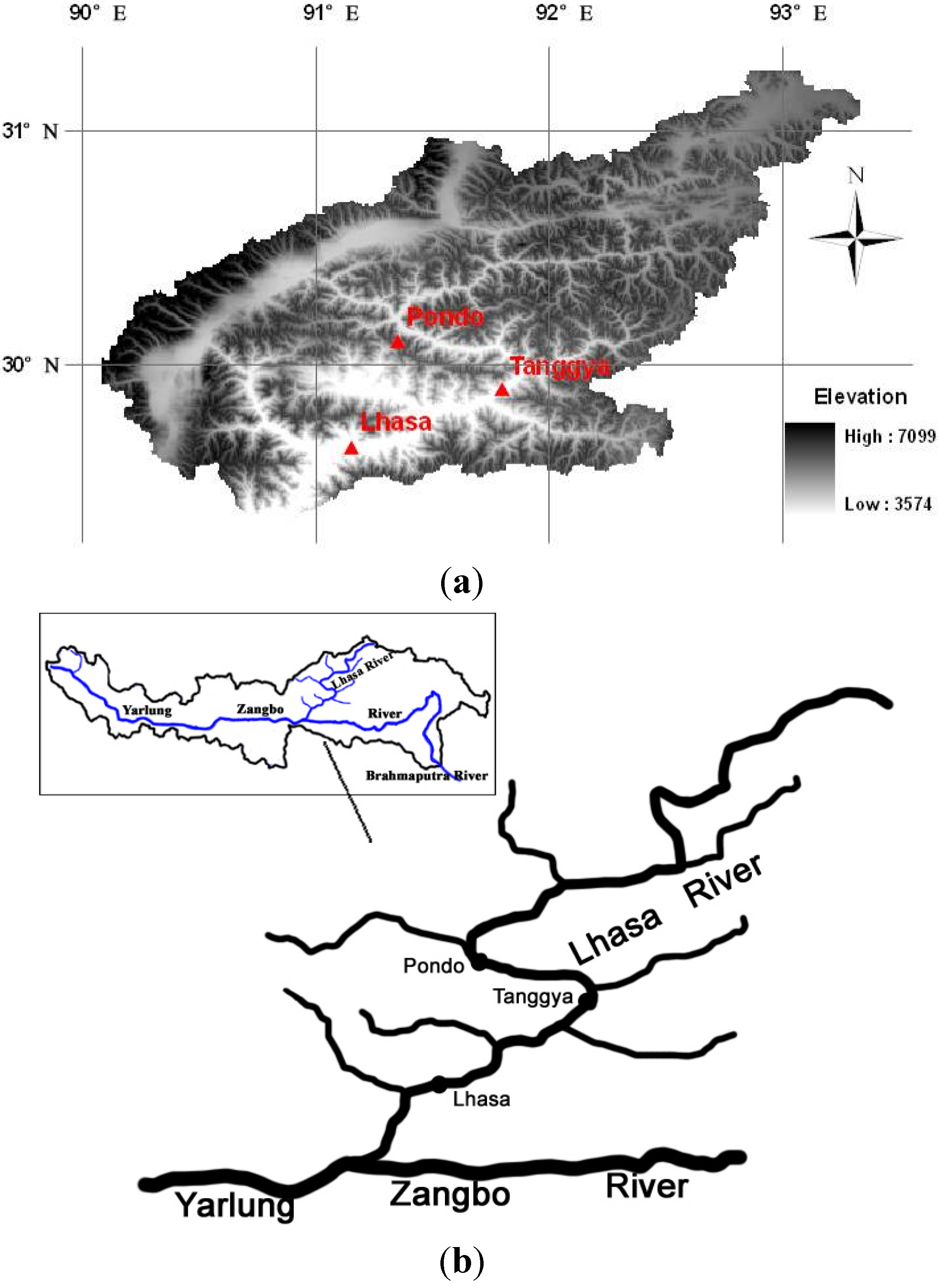
Located in southwestern China, the Lhasa River (Figure 1) is the longest tributary of the Yarlung Zangbo River, with a mainstream length of approximately 551 km. The river originates at Nyangqentanglha Mountain on the Qinghai-Tibet Plateau [15]. The Lhasa River basin has an area of 26,225 km², and its elevation ranges from 3580 to 7000 m, with an average gradient of 2.9%. In the Lhasa River basin, stream flow, and weather data are recorded at three hydrological stations located at Pondo, Tanggya, and Lhasa (see Figure 1 and Table 2). The Lhasa station is located near the river outlet. At this station, the average annual precipitation is 427 mm/year, the average annual temperature is 7.7 °C, and the recorded highest and lowest temperatures are 29.5 °C and −18.0 °C, respectively. Rainfall variability during any year is significant, and its distribution is also uneven, with much of the rainfall concentrating during the summer period of June–September. In this basin, snowmelt mainly occurs during April and May [16,17].

Figure 1. (a) Topographic map; (b) the river network of the Lhasa River basin.

Figure 1. (a) Topographic map; (b) the river network of the Lhasa River basin.

Table 2. Information of hydrological stations in the Lhasa River basin.

Hydrological Station	Location	Elevation (m)	Watershed Area (km2)	Mean Annual Precipitation (mm)
Pondo	30°06′ N, 91°21′ E	4050	16,370	530
Tanggya	29°54′ N, 91°48′ E	3850	20,367	520
Lhasa	29°39′ N, 91°09′ E	3670	26,225	447

Table 2. Information of hydrological stations in the Lhasa River basin.

Hydrological Station	Location	Elevation (m)	Watershed Area (km2)	Mean Annual Precipitation (mm)
Pondo	30°06′ N, 91°21′ E	4050	16,370	530
Tanggya	29°54′ N, 91°48′ E	3850	20,367	520
Lhasa	29°39′ N, 91°09′ E	3670	26,225	447

Several studies have been conducted to investigate the hydrological processes and water resources of the Qinghai-Tibet Plateau region. Wu et al. [18] applied three methods (the artificial neural network model, the staging calm auto-regressive model and the seasonal auto-regressive model) to a 41-year (1956 to 1968 and 1973 to 2000) average of monthly stream flow data in the Lhasa River and found the artificial neural network model to perform the best at simulating stream flow. In the Niyang River (one of the major tributaries of the Yarlung Zangbo River), a flood forecasting model was developed based on the black-box method using a mixed linear regression model [19]. The model was calibrated using the hydrological data of 1997–2002 during the flood season, and verified using the hydrological data observed in 2003. The results showed that the model could be used for flood forecasting. Furthermore, Zhang et al. [20] used CC (cascade correlation) and BP (back propagation) models to forecast the monthly stream flow in the Lhasa River. Such studies have mainly focused on statistical analysis of hydrological and meteorological time series, and there is a general lack of application of physically-based hydrological models to the Yarlung Zangbo River basin, especially the Lhasa River basin.

3. Data and Methodology

3.1. Research Data

In the Lhasa River basin, hydrological data measurements are very limited. There are only three hydrological stations, namely Pondo, Tanggya, and Lhasa (see Figure 1 and Table 2). In this study, hourly precipitation and stream flow and daily pan evaporation data observed during the summer (June–September) for the period of 1998–2000 are considered. To investigate the skill of the model in forecasting flood flows in the Lhasa River, this study focuses on the simulation of summer stream flow from 12 June to 30 September, which is the river flood season. Similar to the study of Chen and Kumar [21], digital elevation model (DEM) data with a resolution of 1 km in the Lhasa River basin are extracted from a global DEM dataset (Global Land One-kilometre Base Elevation, National Geophysical Data Center, NOAA), and then the topographic index for TOPMODEL is derived.

It should be noted that the TOPMODEL version used in this study does not include a snowmelt module because the study period is summer (i.e., from 12 June to 30 September), as snow melt occurs only during April and May in this region. To evaluate the influence of snow melt in runoff generation, we investigate the variation of the snow coverage in the study area in the summer. Similar to Chen and Sun [22], the available MODIS (moderate resolution imaging spectroradiometer) snow cover data (approximately 160 remote sensing images obtained from ftp://n4ftl01u.ecs.nasa.gov) from June to September during the period of 2000–2010 are analyzed. It is worth noting that the MODIS data became available in 2000. From the analysis of the MODIS data, we find that the average snow cover is approximately 6% of the study area from June to September during the period of 2000–2010, and the inter-annual variation of the percentage of snow cover is small. Therefore, it can be deduced that rainfall in summer is a dominant factor in generating summer stream flow in the Lhasa River basin, and for simplicity, only rainfall data are used to simulate stream flow.

3.2. TOPographic Model (TOPMODEL)

TOPographic Model (TOPMODEL) adopts a topographic index to represent a dynamic saturated area of a basin [1,3,4]. For a grid cell of DEM data, i, its topographic index, TI_i, is calculated as follows:

$$T{I}_i=\ln \frac{a_i}{\tan {\text{β}}_i}$$

(1)

where a_i is the area of the hillslope per unit contour length, and tanβ_i is the local surface slope at grid cell i.

In TOPMODEL, the surface runoff at grid i at time t is calculated as follows [2,23]:

$$q_{is}(t)=S_{uz}(t)-S{D}_i(t)$$

(2)

where $S_{uz}$ is the storage in the unsaturated zone and $SD$ is the local storage deficit.

$$S{D}_i\left(t\right)=Sbar\left(t\right)-S_{zm}\cdot \left[T{I}_i-{\text{λ}}^{*}\right]$$

(3)

In the above equation, $Sbar$ is the average storage deficit over the whole basin, $S_{zm}$ is the maximum moisture deficit in the unsaturated zone, ${\text{λ}}^{*}=\frac{1}{A}{\displaystyle \underset{A}{\int }T{I}_{i}dA}$ is an average of the topographic indices in the basin, and $A$ is the basin area. Using the topographic index and other TOPMODEL parameters, the base flow, q_b, can be calculated as follows [2,23]:

$$q_b\left(t\right)=q_0{e}^{-Sbar\left(t\right)/S_{zm}}$$

(4)

where q₀ is equal to $A{T}_0{e}^{-{\text{λ}}^{*}}$and $T_0$ is the lateral transmissivity when the soil column is saturated.

3.3. Original Routing Algorithm

The original routing algorithm for TOPMODEL [1] consists of two parts. The first part is to compute the travel time of runoff from any grid cell to a sub-basin outlet, and the second part is to compute the travel time of runoff in channels from upstream to downstream. For the first part, a flow delay function is normally represented by using a distance-related method. The time taken for runoff to reach a sub-basin outlet from any grid cell is calculated by the equation given below [23]:

$$t_j={\displaystyle \sum _{i=1}^M\frac{x_i}{\text{ν}\tan {\text{β}}_i}}$$

(5)

where $t_j$ is the time delay (in units of hours; noted as h hereafter) for runoff from the grid cell $j$, $x_i$ is the flow path length (m), $\text{ν}$ is the flow velocity (m/h), and M is the number of the segments between the grid cell $j$ and the sub-basin outlet. For the second part (i.e., the channel routing component), a simple nonlinear algorithm is normally used to compute $c_t$, an average kinematic wave velocity for a river channel:

$$c_t=CHA\cdot Q_t^{CHB}$$

(6)

where $Q_t$ is the discharge at time $t$, and $CHA$ and $CHB$ are coefficients, which can be calibrated. The travel time of runoff in a channel from an upstream gauge to a downstream gauge can be calculated using the length of the channel and $c_t$. This approach is an explicit approximation to a kinematic wave channel routing algorithm [23]. Most applications of this original routing algorithm have been based on a simple constant wave speed routing algorithm.

3.4. New Routing Algorithm

For a sparsely-gauged river basin, a sub-basin for computing the first part of runoff travel time using Equation (5) is usually larger, and the assumption of a constant flow velocity v is not reliable; in addition, the channel length from an upstream gauge to a downstream gauge is rather long, and the assumption of a constant wave speed for routing algorithms is not rational. To relax these two assumptions for sparsely-gauged river basins, this paper adopts the UH method to route the overland flow [24]:

$$Q_s(t)={\displaystyle \sum _{k=1}^m{q}_s(t-k+1)UH(k)}$$

(7)

where $UH(k)$ is a unit hydrograph, k is the interval index, and m is the number of intervals with non-zero effective rainfall. There is a relationship between UH and Nash’s instantaneous unit hydrograph [24], given by

$$IUH(k)=\frac{3.6\Delta t}{A}UH(k)$$

(8)

where $IUH(k)$ is Nash’s instantaneous unit hydrograph, and $\Delta t$ is the time interval. The mathematical form for Nash’s instantaneous unit hydrograph is equivalent to the gamma distribution [25]:

$$IUH(k)=\frac{1}{w\Gamma (N)}{(\frac{k}{w})}^{N-1}{e}^{-\frac{k}{w}}$$

(9)

where $N$ is the number of linear reservoirs in a series, w is the storage coefficient, and $\Gamma (N)$ is the gamma function ($\Gamma (N)=(N-1)!$ for integer value of $N$). According to Nash’s instantaneous unit hydrograph and Equation (8), a UH can be obtained, and then the overland flow can be computed by substituting UH into Equation (7).

Furthermore, the linear reservoir method is used to route the base flow, q_b, which is computed by Equation (4), and the routed base flow, Q_g, is calculated as follows:

$$Q_g(t)=K_g{Q}_g(t-1)+(1-K_g)q_b(t)$$

(10)

where $K_g$ is the groundwater recession coefficient. Then, the total routed runoff can be computed by the equation below:

$$Q(t)=Q_s(t)+Q_g(t)$$

(11)

To use the new routing algorithm, the parameters of $N$, w and $K_g$ require calibration.

3.5. Criteria for Evaluating Model Performance

The first criterion used in this study to evaluate the model performance is the Nash-Sutcliffe efficiency index [26], which is defined as follows:

$$NE=1-\frac{{\displaystyle \sum _t{(Q_t^o-Q_t^s)}^2}}{{\displaystyle \sum _t{(Q_t^o-{\overline{Q}}_o)}^2}}$$

(12)

where $Q_t^o$ is the observed stream flow, $Q_t^s$ is the simulated stream flow, and ${\overline{Q}}_o$ is the mean value of the observed stream flow. The value of NE is equal to unity if the simulation matches the observation perfectly.

The second efficiency criterion used is the relative error of the volumetric fitness between the observed and simulated stream flow series and is defined by:

$$R_E=\frac{{\displaystyle \sum _t{Q}_t^s}-{\displaystyle \sum _t{Q}_t^o}}{{\displaystyle \sum _t{Q}_t^o}}\times 100\%$$

(13)

The value of $R_E$ is zero if the total volume of the simulated stream flow is equal to that of the observed ones.

The third criterion is the correlation coefficient, r, to evaluate the match of variations between observations and simulations. The equation for computing r is given as

$$r=\frac{{\displaystyle \sum _t\left(Q_t^o-{\overline{Q}}_o\right)\left(Q_t^s-{\overline{Q}}_s\right)}}{\sqrt{{\displaystyle \sum _t{\left(Q_t^o-{\overline{Q}}_o\right)}^2}{\displaystyle \sum _t{\left(Q_t^s-{\overline{Q}}_s\right)}^2}}}$$

(14)

where ${\overline{Q}}_s$ is the mean value of the simulated stream flow. For model calibration in this study, the Simplex algorithm [27] is used.

Because the simulation is conducted from 12 June to 30 September for the period of data considered (1998–2000), rainfall serves as the driving force for floods, as snowmelt only occurs during April and May. In addition, in the study area, because the flood in the summer of 1998 was the largest flood during the study period, the observed stream flows in 1998 are chosen for verification purposes to better assess the skill of the model in stream flow simulation, especially regarding the flood flows. The floods that occurred during the summer of 1999–2000 are used for calibration. It should be noted that the time interval used in this study is one hour.

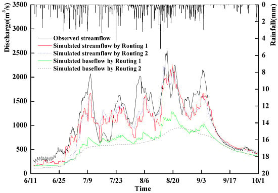
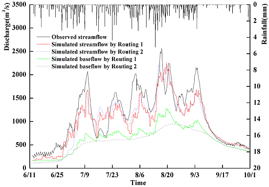
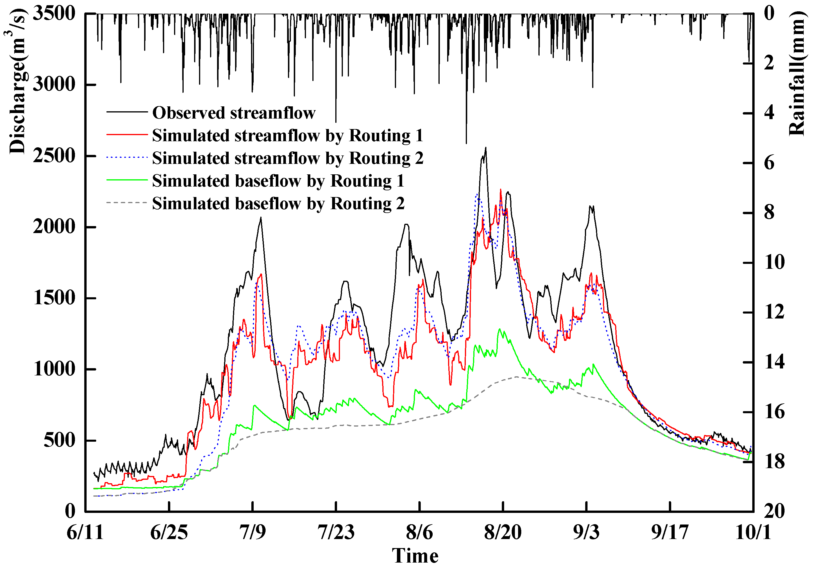
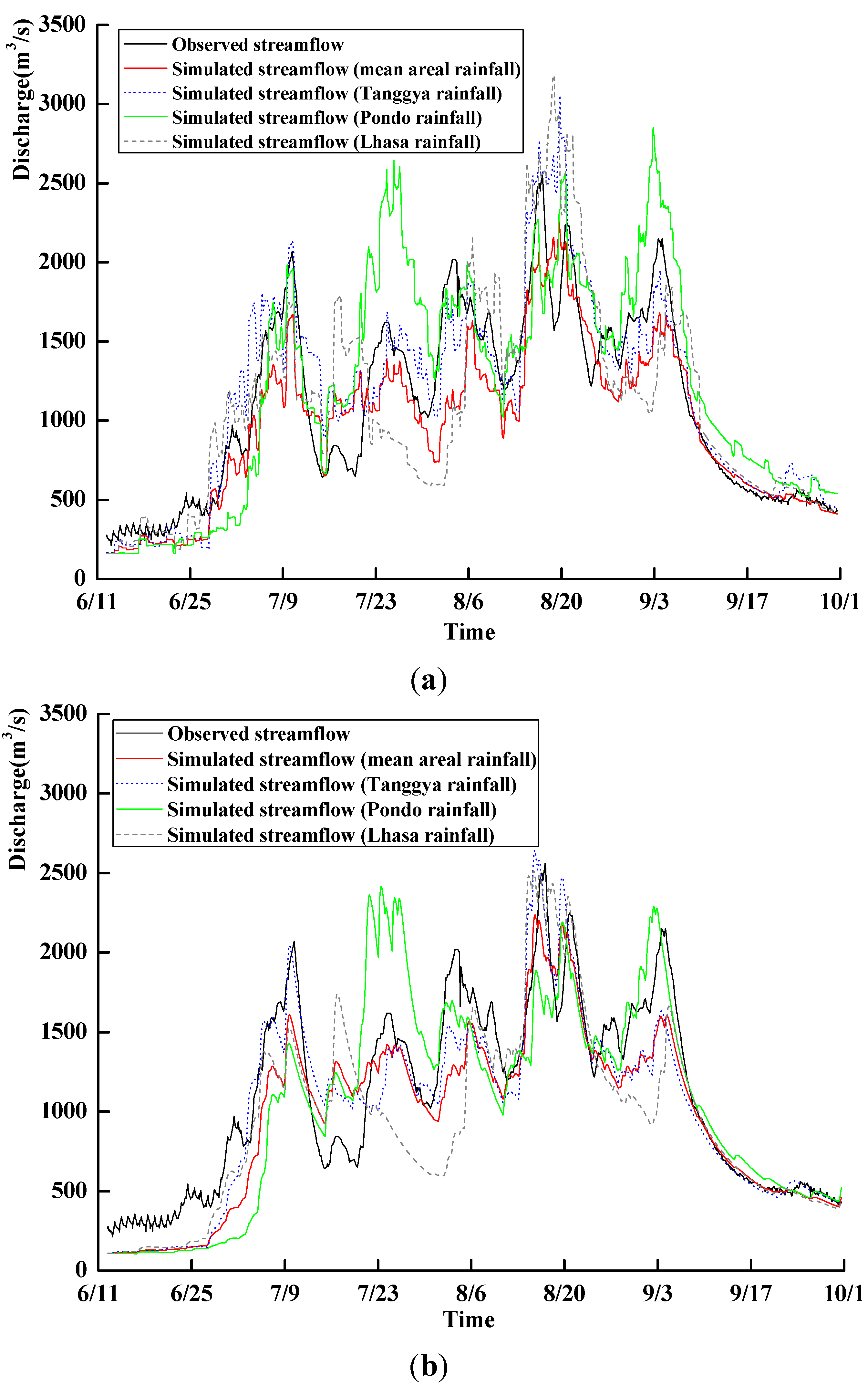
4. Results and Discussion

Because there are only three hydrological stations available in the Lhasa River basin (i.e., the Pondo, Tanggya and Lhasa stations) despite its large area, the basin is separated into three parts in association with these stations. Accordingly, the topography indices for these three sub-basins are calculated. In the new routing algorithm, the values of new three parameters (N, w and K_g) are 16, 3.3 and 0.00033, respectively.

Table 3 lists the stream flow simulation results obtained for the Lhasa station using TOPMODEL and the two routing algorithms mentioned above. Here, Routing 1 and Routing 2 refer to the original and new routing algorithms, respectively. And the average hourly precipitation data at three hydrological stations (namely Pondo, Tanggya, and Lhasa) was used in the simulations. Table 3 shows that the Nash-Sutcliffe efficiencies, NE, obtained using both the routing algorithms are between 0.70 and 0.78, the relative errors of the volumetric fitness, $R_E$, are between −12% and 9%, and the correlation coefficients, r, are between 0.85 and 0.91. Comparison of NE, R_E and r reveals that the performances of TOPMODEL with the original and new routing algorithms are similar.

Table 3. Simulation results by using TOPMODEL and the original and new routing algorithms.

Period	Year	Routing 1			Routing 2
		NE	RE (%)	r	NE	RE (%)	r
Calibration	1999	0.76	5	0.89	0.73	9	0.87
	2000	0.70	−6	0.85	0.77	−5	0.90
Verification	1998	0.77	−12	0.91	0.78	−12	0.91

Note: Routings 1 and 2 refer to the original and new routing algorithms for TOPMODEL, respectively.

Table 3. Simulation results by using TOPMODEL and the original and new routing algorithms.

Period	Year	Routing 1			Routing 2
		NE	RE (%)	r	NE	RE (%)	r
Calibration	1999	0.76	5	0.89	0.73	9	0.87
	2000	0.70	−6	0.85	0.77	−5	0.90
Verification	1998	0.77	−12	0.91	0.78	−12	0.91

Note: Routings 1 and 2 refer to the original and new routing algorithms for TOPMODEL, respectively.

Table 4 lists the observation and simulation results of several flood peaks that occurred at the Lhasa station from June to September in the study period. The relative errors between the observed and simulated flood peaks are mostly in the range of −22% to 19%, and the performances of both methods are also similar.

Table 4. Simulation results for major flood peaks at Lhasa station.

Period	Year	Observed Peak Flow		Simulated Peak Flow by Routing 1			Simulated Peak Flow by Routing 2
		Time (MM-DD h)	Discharge (m3/s)	Time (MM-DD h)	Discharge (m3/s)	Relative Error (%)	Time (MM-DD h)	Discharge (m3/s)	Relative Error (%)
Verification	1998	07-10 10:00	2070	07-10 11:00	1671	−19	07-09 17:00	1608	−22
	1998	08-17 02:00	2560	08-19 15:00	2267	−11	08-15 14:00	2236	−13
Calibration	1999	06-30 20:00	1190	07-02 19:00	1140	−4	07-03 08:00	1014	−15
	1999	09-02 00:00	1590	08-31 16:00	1659	4	08-31 16:00	1715	8
	2000	08-03 10:00	1610	08-03 15:00	1915	19	08-03 10:00	1774	10
	2000	08-24 00:00	1930	08-22 22:00	1836	−5	08-22 17:00	1828	−5

Table 4. Simulation results for major flood peaks at Lhasa station.

Period	Year	Observed Peak Flow		Simulated Peak Flow by Routing 1			Simulated Peak Flow by Routing 2
		Time (MM-DD h)	Discharge (m3/s)	Time (MM-DD h)	Discharge (m3/s)	Relative Error (%)	Time (MM-DD h)	Discharge (m3/s)	Relative Error (%)
Verification	1998	07-10 10:00	2070	07-10 11:00	1671	−19	07-09 17:00	1608	−22
	1998	08-17 02:00	2560	08-19 15:00	2267	−11	08-15 14:00	2236	−13
Calibration	1999	06-30 20:00	1190	07-02 19:00	1140	−4	07-03 08:00	1014	−15
	1999	09-02 00:00	1590	08-31 16:00	1659	4	08-31 16:00	1715	8
	2000	08-03 10:00	1610	08-03 15:00	1915	19	08-03 10:00	1774	10
	2000	08-24 00:00	1930	08-22 22:00	1836	−5	08-22 17:00	1828	−5

Figure 2 shows the observed hourly stream flow and simulated hourly base flows and stream flows for the Lhasa station in the year 1998. Both the original and new routing algorithms can simulate the rising and recessing limbs of the stream flows reasonably well in comparison to the observed flood hydrograph. The new algorithm is insensitive to input, therefore the simulated base flow using the new routing algorithm is smoother than that using the original routing algorithm. Due to sparse data currently in the basin, it is not easy to determine quantity and proportion of base flow in the stream flow. For the further research, isotop experiments [28,29] could be tested in the stream flow, and the actual amount of base flow would remain clear.

The correlation coefficient results obtained for stream flows from 12 June to 30 September for the study period (see Table 3) do not offer a strong indication as to the better routing algorithm (i.e., the new routing algorithm or the original one). However, the use of correlation coefficients can be better presented by examining the stable or rapid variations of stream flow simulated by the two routing algorithms. Table 5 lists the correlation coefficients for flood events in each year, for a total of 11 events over the three-year study period (1998–2000). The results show that the correlation coefficients of simulated stream flow from the new routing algorithm are mostly larger than those from the original routing algorithm; specifically, for a flood hydrograph that occurred during 15–17 August 1998, values of 0.59 and 0.71 were found for the original and new algorithms, respectively. Therefore, intuitively, the linear reservoir and the UH method used in the new routing algorithm are more reliable for the Lhasa River basin when compared to the original routing algorithm.

Figure 2. Observed and simulated hourly stream flow and base flow at Lhasa in 1998.

Figure 2. Observed and simulated hourly stream flow and base flow at Lhasa in 1998.

Table 5. Correlation coefficients for flood events occurred at Lhasa station from 1998 to 2000.

Time	Correlation Coefficient
	Routing 1	Routing 2
5 July 1998 04:00 to 12 July 1998 16:00	0.81	0.83
21 July 1998 10:00 to 28 July 1998 18:00	0.62	0.73
31 July 1998 13:00 to 10 August 1998 00:00	0.60	0.72
15 August 1998 20:00 to 17 August 1998 18:00	0.59	0.71
24 August 1998 20:00 to 7 September 1998 17:00	0.69	0.89
22 August 1999 05:00 to 26 August 1999 15:00	0.63	0.70
28 August 1999 02:00 to 7 September 1999 04:00	0.84	0.84
12 September 1999 11:00 to 20 September 1999 01:00	0.65	0.68
1 August 2000 10:00 to 9 August 2000 00:00	0.82	0.83
19 August 2000 00:00 to 31 August 2000 06:00	0.86	0.88
12 September 2000 11:00 to 20 September 2000 01:00	0.72	0.75

Table 5. Correlation coefficients for flood events occurred at Lhasa station from 1998 to 2000.

Time	Correlation Coefficient
	Routing 1	Routing 2
5 July 1998 04:00 to 12 July 1998 16:00	0.81	0.83
21 July 1998 10:00 to 28 July 1998 18:00	0.62	0.73
31 July 1998 13:00 to 10 August 1998 00:00	0.60	0.72
15 August 1998 20:00 to 17 August 1998 18:00	0.59	0.71
24 August 1998 20:00 to 7 September 1998 17:00	0.69	0.89
22 August 1999 05:00 to 26 August 1999 15:00	0.63	0.70
28 August 1999 02:00 to 7 September 1999 04:00	0.84	0.84
12 September 1999 11:00 to 20 September 1999 01:00	0.65	0.68
1 August 2000 10:00 to 9 August 2000 00:00	0.82	0.83
19 August 2000 00:00 to 31 August 2000 06:00	0.86	0.88
12 September 2000 11:00 to 20 September 2000 01:00	0.72	0.75

Because the observed rainfall at the three hydrological stations (Pondo, Tanggya, and Lhasa) can not sufficiently represent the spatial variation of precipitation over the Lhasa River basin, a sensitivity analysis of the influence of rainfall spatial variation on hourly stream flow simulation is also performed. To this end, four rainfall time series, corresponding to the rainfall recorded at Pondo, Tanggya, Lhasa and their average, are used to represent the rainfall of the whole study area. Figure 3 shows the simulation results of the 1998 summer stream flow at the Lhasa station obtained by using these four rainfall series. The results obtained using the original routing algorithm (Figure 3a) show that a significant difference exists between the observed and the simulated hourly stream flow at the Lhasa station from June to September, 1998. Additionally, the simulated stream flow using the rainfall recorded at the Pondo station significantly overestimates most flood peaks, such as the floods that occurred on 26 July and 7 September. The results further indicate that, among the four rainfall time series considered, the average rainfall of the three stations provide the best stream flow simulation. Figure 3b presents the stream flow simulated results obtained using the new routing algorithm. Compared with the simulations presented in Figure 3a, the simulated stream flows in Figure 3b are more stable. These results are similar to those presented in Figure 2 and Table 5.

Figure 3. Observed and simulated hourly stream flow at Lhasa in 1998 by using (a) Routing 1; and (b) Routing 2 based on the different rainfall scenarios.

Figure 3. Observed and simulated hourly stream flow at Lhasa in 1998 by using (a) Routing 1; and (b) Routing 2 based on the different rainfall scenarios.

Figure 3b shows that the simulated stream flows at the outlet of the basin using the rainfall recorded at the Tanggya station based on TOPMODEL are mostly comparable to the observed stream flows. In fact, because the stream flow at the Lhasa station is more closely related to that of the Tanggya station, the Tibetan Bureau of Hydrology (TBH) [30] has developed a correlation diagram method for the Lhasa River on the basis of experience. This diagram has also been used to predict the water level at the Lhasa station, according to the water level relationship between the Lhasa station and the Tanggya station. The simulation results in Figure 3b confirm such a relationship developed by TBH.

5. Conclusions

Although TOPMODEL has been widely applied to different river basins around the world, such applications have mostly been focused on small basins and data-rich large basins, and there is a lack of application to sparsely-gauged large river basins. In this study, a new routing algorithm was developed for routing the runoff for a relatively longer channel from the upstream station to the downstream one, and both the original and new routing algorithms were used in TOPMODEL in its application to the Lhasa River basin, a sparsely-gauged large basin. Hourly summer stream flow from June to September was simulated. The results for major summer flood peaks at the Lhasa station for the period from 1998 to 2000 were analyzed. In addition, the influence of rainfall spatial variations on stream flow simulation was investigated. The major conclusions drawn from this study are as follows:

1. Application of the original and new routing algorithms to the sparsely gauged Lhasa River basin reveals that the new routing algorithm is suitable for the study area. Furthermore, comparison of the simulated base flows obtained from the original and new routing algorithms showed that the new algorithm can provide a smoother hourly base flow than the original routing algorithm.

2. The simulated stream flows from both the original and new routing algorithms indicate that the three stations available (Pondo, Tanggya, and Lhasa) are not sufficient to represent the rainfall spatial variation in the study area. To evaluate the influence of the spatial variation of rainfall, the mean areal rainfall time series was also used to calibrate the model parameters and the corresponding simulated stream flow from the model were considered as a reference. The rainfall recorded at Pondo, Tanggya, and Lhasa hydrological stations were used as inputs to the model with the mean areal rainfall model parameters, respectively. The simulated stream flow was compared with mean areal rainfall. The results reveal that the hourly stream flow at the outlet of the basin simulated by only using the rainfall recorded at Tanggya station are mostly comparable to the observed stream flow in the same location.

3. In this study, only rainfall data were used to drive TOPMODEL and its related routing algorithms. For a large plateau basin, such as the Lhasa River basin, the snow cover is mostly present throughout the year, and thus, snowmelt can contribute to runoff generation. To investigate the snow cover influence using the available MODIS snow cover data, we found that the average snow cover accounts for approximately 6% of the Lhasa River basin from June to September, and the inter-annual variation of snow cover in the summer is small. Therefore, we assumed that rainfall is a dominant force in generating summer stream flows and that snowmelt is not a particularly important factor. Nevertheless, it would be interesting to study the influence of snowmelt on stream flow simulation throughout the entire year. We will investigate this aspect in our future research.

References

1. Beven, K.J.; Kirkby, M.J. A physically based variable contributing area model of basin hydrology. Hydrol. Sci. Bull. 1979, 24, 43–69. [Google Scholar] [CrossRef]
2. Beven, K.J.; Lamb, R.; Quinn, P.F.; Romanowicz, R.; Freer, J. TOPMODEL. In Computer Models of Watershed Hydrology; Singh, V.P., Ed.; Water Resources Publications: Highlands Ranch, CO, USA, 1995; pp. 627–668. [Google Scholar]
3. Murphy, J.C.; Knight, R.R.; Wolfe, W.J.; Gain, W.S. Predicting ecological flow regime at ungaged sites: A comparison of methods. River Res. Appl. 2013, 29, 660–669. [Google Scholar] [CrossRef]
4. Zhu, D.; Peng, D.Z.; Cluckie, I.D. Statistical analysis of error propagation from radar rainfall to hydrological models. Hydrol. Earth Syst. Sci. 2013, 17, 1445–1453. [Google Scholar] [CrossRef]
5. Peng, D.Z.; Xu, Z.X.; Qiu, L.H.; Zhao, W.M. Distributed rainfall-runoff simulation for an unclosed river basin with complex river system: A case study of lower reach of the Wei River, China. J. Flood Risk Manag. 2014, 2014. [Google Scholar] [CrossRef]
6. Choi, H.T.; Beven, K.J. Multi-Period and multi-criteria model conditioning to reduce prediction uncertainty in an application of TOPMODEL within the GLUE framework. J. Hydrol. 2007, 332, 316–336. [Google Scholar] [CrossRef]
7. Gallart, F.; Latron, J.; Llorens, P.; Beven, K.J. Using internal catchment information to reduce the uncertainty of discharge and baseflow predictions. Adv. Water Resour. 2007, 30, 808–823. [Google Scholar] [CrossRef]
8. Beven, K.J.; Freer, J. A dynamic TOPMODEL. Hydrol. Process. 2001, 15, 1993–2011. [Google Scholar] [CrossRef]
9. Page, T.; Beven, K.J.; Freer, J.; Neal, C. Modelling the chloride signal at Plynlimon, Wales, using a modified dynamic TOPMODEL incorporating conservative chemical mixing (with uncertainty). Hydrol. Process. 2007, 21, 292–307. [Google Scholar] [CrossRef]
10. Wu, S.; Li, J.; Huang, G.H. Modeling the effects of elevation data resolution on the performance of topography-based watershed runoff simulation. Environ. Model. Softw. 2007, 22, 1250–1260. [Google Scholar] [CrossRef]
11. Cameron, D. An application of the UKCIP02 climate change scenarios to flood estimation by continuous simulation for a gauged catchment in the northeast of Scotland, UK (with uncertainty). J. Hydrol. 2006, 328, 212–226. [Google Scholar] [CrossRef]
12. Chiang, S.; Tachikawa, Y.; Takara, K. Hydrological model performance comparison through uncertainty recognition and quantification. Hydrol. Process. 2007, 21, 1179–1195. [Google Scholar] [CrossRef]
13. Clark, D.B.; Gedney, N. Representing the effects of subgrid variability of soil moisture on runoff generation in a land surface model. J. Geophys. Res. 2008, 113. [Google Scholar] [CrossRef] [Green Version]
14. Seibert, J.; Bishop, K.H.; Nyberg, L. A test of TOPMODEL’s ability to predict spatially distributed groundwater levels. Hydrol. Process. 1997, 11, 1131–1144. [Google Scholar] [CrossRef]
15. Huang, X.; Sillanpaa, M.; Gjessing, E.T.; Peraniemi, S.; Vogt, R.D. Water quality in the southern Tibetan Plateau: Chemical evaluation of the Yarlung Tsangpo (Brahmaputra). River Res. Appl. 2011, 27, 113–121. [Google Scholar] [CrossRef]
16. Peng, D.Z.; Du, Y. Comparative analysis of several Lhasa River basin flood forecast models in Yarlung Zangbo River. In Proceedings of the 4th International Conference on Bioinformatics and Biomedical Engineering (iCBBE), Chengdu, China, 18–20 June 2010.
17. Qiu, L.H.; You, J.J.; Qiao, F.; Peng, D.Z. Simulation of snowmelt runoff in the ungauged basin based on MODIS: A case study in Lhasa River basin. Stoch. Environ. Res. Risk Assess. 2014, 28, 1577–1585. [Google Scholar] [CrossRef]
18. Wu, T.; Yuan, P.; Dai, L.; Ding, Y.; Xie, S. Research on the stream flow forecast methods of Tibet Lhasa River. Water Conserv. Sci. Technol. Econ. 2005, 11, 77–79. (In Chinese) [Google Scholar]
19. Zhang, X.Y.; Dong, Z.C.; Wang, J.Q.; Zhao, J.X. Method of flood forecasting for Niyang River Basin of Yarlung Zangbo River. J. Hohai Univ. (Nat. Sci.) 2005, 33, 530–533. (In Chinese) [Google Scholar]
20. Zhang, Z.G.; Xu, Z.X.; Gong, T.L. Cascade-correlation algorithm and its application in monthly stream flow forecasting. Adv. Water Sci. 2007, 18, 114–117. (In Chinese) [Google Scholar]
21. Chen, J.; Kumar, P. Topographic influence on the seasonal and inter-annual variation of water and energy balance of basins in North America. J. Clim. 2001, 14, 1989–2014. [Google Scholar] [CrossRef]
22. Chen, J.; Sun, L. Using MODIS EVI to detect vegetation damage caused by the 2008 ice and snow storms in south China. J. Geophys. Res.-Biogeosci. 2010, 115. [Google Scholar] [CrossRef] [Green Version]
23. Beven, K.J. Rainfall-Runoff Modelling; John Wiley & Sons Ltd.: Chichester, UK, 2001. [Google Scholar]
24. Chow, V.T.; Maidment, D.R.; Mays, L.W. Applied Hydrology; McGraw-Hill Inc.: New York, NY, USA, 1988; pp. 211–213. [Google Scholar]
25. Nash, J.E. The form of the instantaneous unit hydrograph. Int. Assoc. Sci. Hydrol. 1957, 45, 114–121. [Google Scholar]
26. Nash, J.E.; Sutcliffe, J.V. River flow forecasting through conceptual models part I—A discussion of principles. J. Hydrol. 1970, 10, 282–290. [Google Scholar] [CrossRef]
27. Murty, K.G. Linear Programming; John Wiley & Sons Inc.: New York, NY, USA, 1983. [Google Scholar]
28. McDonnell, J.J. A rationale for old water discharge through macropores in a steep, humid catchment. Water Resour. Res. 1990, 26, 2821–2832. [Google Scholar] [CrossRef]
29. Kendall, C.; McDonnell, J.J. Isotope Tracers in Catchment Hydrology; Elsevier Science B.V.: Amsterdam, The Netherlands, 1998. [Google Scholar]
30. Tibetan Bureau of Hydrology. Handbook of Hydrological Forecasting; Tibet Water Resources Department: Lhasa, China, 2000. (In Chinese) [Google Scholar]