Data Assimilation and Modeling Frontiers in Soil–Water Systems

Abstract

Sustainable soil–water management under climate and socio-economic pressures requires predictive capability that is both mechanistic and continuously corrected by observations. Data assimilation (DA) provides the formal machinery to merge models with heterogeneous measurements—from satellite evapotranspiration and soil moisture to cosmic-ray neutron sensing, proximal geophysics, lysimeters, and groundwater hydrographs—while propagating uncertainty. This review (based on 90 references) synthesizes frontiers in DA and modeling for soil–water systems across scales, emphasizing (i) multi-source observation operators and scaling; (ii) coupled crop–vadose–groundwater modeling frameworks and their structural hypotheses; (iii) modern DA methods (ensemble, variational, particle-based, and hybrid physics–ML) for joint estimation of states, parameters, and biases; and (iv) emerging digital twins that enable predict-then-verify management loops for irrigation, recharge enhancement, and drought risk reduction. We highlight how tracer-aided and isotope-informed components can improve evapotranspiration partitioning and recharge threshold detection, and how agent-based or socio-hydrological coupling can represent human decision feedback. Finally, we outline research gaps in uncertainty quantification, benchmarking, reproducibility, and governance needed to operationalize trustworthy soil–water digital twins for resilient food and water systems.

1. Introduction

Global soil and water resources are under unprecedented pressure from population growth, agricultural intensification, and climate change. Water scarcity now affects billions of people worldwide and is recognized as a major threat to socio-economic stability [1,2]. Agriculture is the largest consumer of freshwater and heavily reliant on soil moisture (“green water”), making sustainable soil–water management critical for food security [2,3]. Climate warming exacerbates water shortages: for example, a 3 °C warmer world could expose an additional 150 million hectares of rain-fed cropland to water scarcity [3]. To adapt, strategies that retain more moisture in soils and reduce evaporation could safeguard food production for hundreds of millions of people. These challenges underscore the need for advanced tools that predict water system responses and inform better management.

Integrative modeling and data assimilation (DA) have emerged as powerful approaches for sustainable soil–water management. Process-based models can represent the coupled dynamics of crops, soil moisture, and groundwater, allowing exploration of scenarios for climate adaptation and resource use. However, model predictions carry uncertainties due to imperfect process understanding and variable parameters [4]. DA techniques address this by fusing models with real-world observations (e.g., from satellites and sensors), continually updating model states to improve accuracy [5,6]. Such model–data fusion is increasingly feasible thanks to expanded monitoring networks and computational advances. It enables the creation of digital twins of agro-hydrological systems—virtual replicas of soil–water processes that evolve with observations—that decision-makers can use to test policies in silico before implementation [7].

The importance of these integrated approaches is recognized in the recent literature. For instance, Montanari and Koutsoyiannis [4] argue that embracing uncertainty is unavoidable in hydrology and call for converting deterministic models into stochastic predictors by characterizing model errors [4,8]. Similarly, Clark et al. [5,6] promote modular modeling frameworks that allow multiple process hypotheses to be tested, helping reduce prediction uncertainty through systematic model comparisons. In parallel, the emerging field of socio-hydrology emphasizes modeling human–water interactions, acknowledging that farmer behavior and institutions feed back into hydrological outcomes [9]. This comprehensive review synthesizes advances in observation systems, modeling frameworks, assimilation techniques, and interdisciplinary methods (tracers, socio-hydrologic models, digital twins) for soil–water systems. We highlight case studies across climates—from Chinese farmlands to U.S. irrigated plains and the Indo-Gangetic basin—illustrating real-world applications. We also discuss uncertainty quantification and model validation as foundations for robust risk-based decision making. Finally, we identify research gaps and future directions, including opportunities for new sensors, scalable assimilation, artificial intelligence integration, and ensuring equity and policy relevance in modeling efforts.

In sum, DA and modeling offer a path forward for sustainable soil–water systems by marrying the predictive power of simulation with the grounding of observations. The sections that follow provide a detailed account of the state-of-the-art and best practices in this rapidly evolving field.

2. Advances in Observation Systems

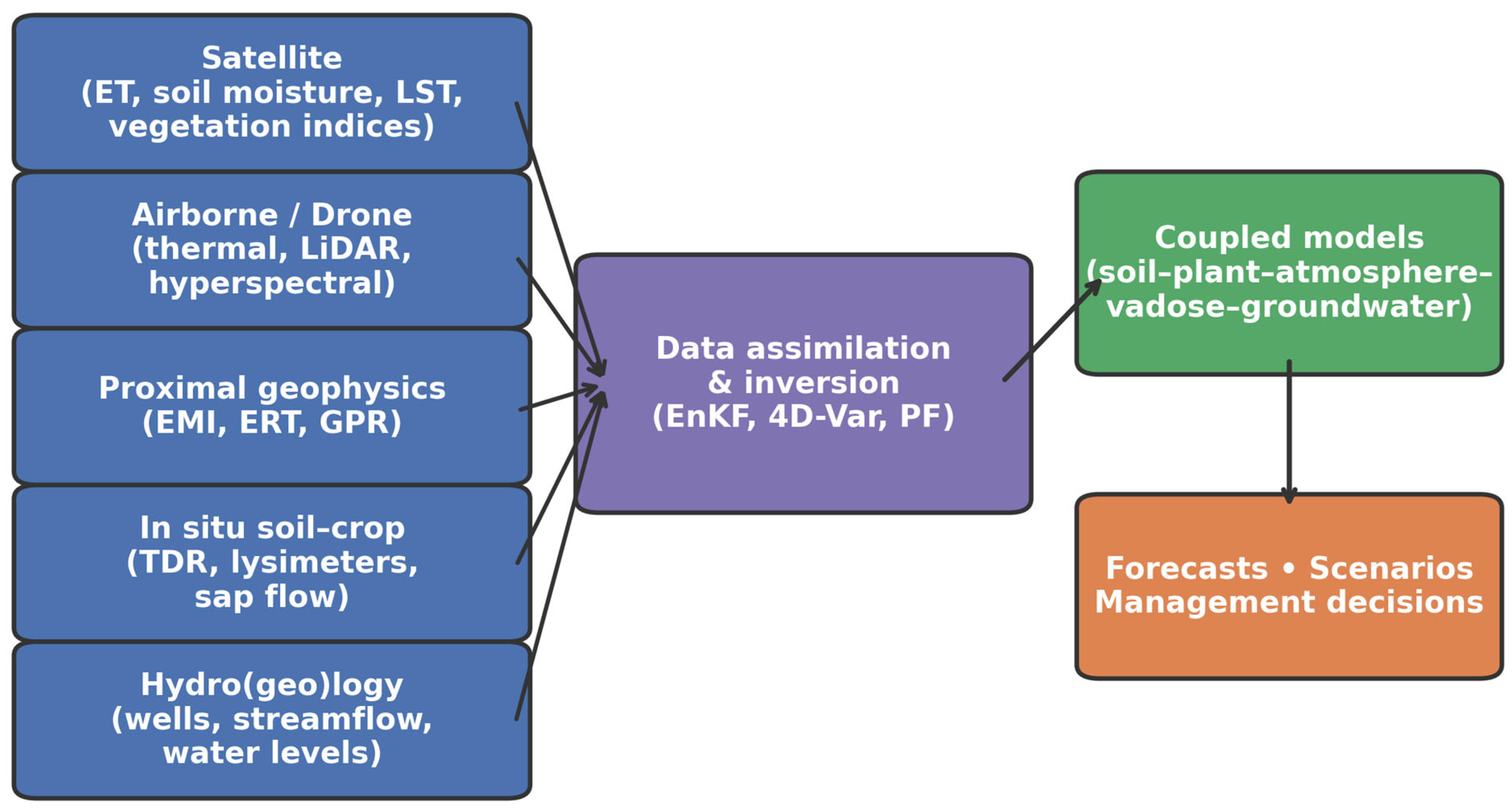
Effective DA requires high-quality observations of the soil–water system. In the past decade, observation technologies have advanced markedly, providing multi-scale data on key variables such as soil moisture, evapotranspiration (ET), and groundwater levels. This section reviews several observation systems—ranging from satellites to in-situ sensors—that have enhanced our ability to monitor soil–water processes for model integration (Figure 1).

Table 1. Observation streams for soil–water DA and typical assimilation strategies.

Observation Stream	Primary Information	Assimilated Target(s)	Common Pitfalls	Suggested DA Strategy
Satellite soil moisture (e.g., SMAP)	Surface wetness (top cm)	Surface & root-zone soil moisture	Depth mismatch; radio-frequency interference; vegetation effects	Bias correction + EnKF with localization; multi-layer update
Satellite ET	Water/energy flux constraint	ET components; root-zone stress	Algorithm uncertainty; cloud gaps; scale mismatch	State augmentation for ET-related parameters; smoothing over windows
Cosmic-ray neutron sensing (CRNS)	Hectare-scale soil moisture	Area-average soil moisture	Calibration to local hydrogen pools; footprint variability	Assimilate as integrated observation with footprint operator
Proximal geophysics (EMI/GPR)	Soil texture/salinity structure proxies	Hydraulic conductivity/texture maps	Non-uniqueness; time-varying salinity	Joint inversion + DA for structural parameters
Lysimeters/flux towers	High-quality water balance and fluxes	ET partitioning; deep percolation	Representativeness; management disturbances	Use for calibration and benchmarking; constrain model bias
Well hydrographs/streamflow	Integrated catchment response	Groundwater storage; baseflow	Human pumping confounding; routing errors	Coupled surface–groundwater DA; multi-objective updates

Note: Data Source: Compiled by the authors based on cited literature. ET = evapotranspiration; SMAP = soil moisture active passive; DA = data assimilation; EMI = electromagnetic induction; GPR = ground-penetrating radar; CRNS = cosmic-ray neutron sensing; EnKF = ensemble Kalman filter.

provides a practical checklist of observation types, their primary information content, and recommended DA strategies across scales.

2.1. Satellite-Based Evapotranspiration and Soil Moisture

Satellite remote sensing now offers near-real-time coverage of land surface water fluxes. Multiple global ET datasets are available, derived from thermal and optical sensors (e.g., MODIS, Landsat) and process algorithms [10]. These products provide daily or weekly estimates of ET at resolutions of tens of kilometers down to sub-kilometer scales [7]. For instance, NASA’s ECOsystem Spaceborne Thermal Radiometer Experiment on Space Station (ECOSTRESS) and the MOD16 ET product together enable monitoring of crop water use and drought stress [7,11]. Such satellite ET data are crucial for agriculture and water management, allowing drought forecasting and irrigation planning on regional to global scales [7,11]. Meanwhile, dedicated satellite missions measure soil moisture directly. The NASA SMAP mission (Soil Moisture Active Passive) has provided global soil moisture maps at ~10 km resolution since 2015. SMAP observes microwave emissions sensitive to the top ~5 cm of soil, capturing surface moisture dynamics [12]. Its data, when assimilated into models, significantly improve soil moisture estimates and hydrologic forecast skill. For example, assimilating SMAP observations into a land surface model reduced soil moisture root-mean-square error and improved the timing of simulated streamflow peaks [12]. Other satellite sensors (ASCAT scatterometer, Sentinel-1 radar) complement SMAP by providing soil moisture at different depths or finer spatial scales. The integration of these satellite products has effectively created a quasi-global soil moisture observing system, filling the gaps of sparse ground networks.

2.2. Cosmic-Ray Neutron Sensing (CRNS)

At intermediate scales (hectares), cosmic-ray neutron sensors have emerged as an innovative tool for soil moisture monitoring. CRNS devices measure fast neutrons above the land surface, which are inversely related to hydrogen content (hence soil water) in the top ~0.3–0.5 m of soil [13]. A single CRNS station can continuously monitor area-average soil moisture over a footprint of up to 200–300 m radius, bridging the scale between point sensors and satellite pixels [13]. The method is non-invasive and low-maintenance, making it attractive for agricultural fields and remote sites. Over the last decade, national networks (e.g., COSMOS in the US, COSMOS-UK, and others) have deployed hundreds of CRNS probes. These networks provide real-time soil moisture data that can be assimilated into hydrological models and used to validate satellite retrievals. Recent technical improvements, such as helium-3-free neutron detectors and standardized calibration under the Soils Moisture Metrology (SoMMet) consortium, are enhancing CRNS reliability and scalability [14]. CRNS data have been successfully used in applications like irrigation scheduling and drought assessment. Still, challenges remain (e.g., correcting for biomass and soil chemistry effects), especially in heterogeneous or irrigated landscapes where the CRNS footprint may encompass mixed conditions.

2.3. Electromagnetic Induction (EMI) and Geophysical Sensors

Geophysical techniques like EMI are increasingly used for mapping soil moisture and subsurface properties. EMI sensors induce electromagnetic fields in the ground and measure the response, which is sensitive to soil electrical conductivity and thus moisture content. They can be deployed on sleds or drones to survey fields and infer the spatial variation of soil moisture to depths of a few meters. EMI surveys provide high-resolution horizontal patterns of wetness, useful for identifying zones of preferential flow, salinity, or variable soil texture that impact infiltration. Additionally, ground-penetrating radar (GPR) and electrical resistivity tomography (ERT) have become practical tools to image moisture in the vadose zone. These tools are collectively known as hydrogeophysics, and their application has expanded to improve understanding of subsurface processes across scales [15]. For example, time-lapse ERT can monitor wetting fronts and drainage in the root zone, offering insight into percolation and recharge events. The integration of hydrogeophysical data with hydrologic models (via coupled inversion or assimilation) is a promising frontier for constraining soil hydraulic parameters and heterogeneity [15].

2.4. Lysimeters and Field Flux Measurements

While remote sensing and proximal sensors cover large areas, lysimeters remain irreplaceable for precise water balance measurements at point to plot scale. Weighing lysimeters directly measure ET by tracking the mass change of an isolated soil–plant monolith, providing high-accuracy ET data for model calibration [16]. Modern lysimeter facilities automate data collection and can quantify daily or even hourly ET, allowing partitioning of evaporation vs. transpiration under controlled conditions. Combined with eddy covariance flux towers (which measure actual ET and energy fluxes over landscapes), lysimeter observations help validate remote sensing ET algorithms and land surface model outputs [11]. They also serve as ground truth for new sensor technologies (e.g., validating CRNS soil moisture against deep lysimeter percolation). Furthermore, well hydrographs (continuous groundwater level records) are a key observation for the soil–water system, linking vadose zone processes to aquifer responses. Dense monitoring of well levels, often available via government databases, permits tracking of groundwater trends, recharge events, and irrigation pumping impacts. Assimilation of well observations into coupled vadose–groundwater models can greatly improve simulation of water table dynamics and inform sustainable yield estimates [17].

In summary, an array of complementary observation systems is now available for soil–water monitoring. Satellites provide broad coverage of surface fluxes and moisture, ground sensors like CRNS and EMI offer intermediate-scale detail, and in-situ instruments yield high-fidelity point data. These multi-scale observations set the stage for advanced modeling frameworks that can ingest data at various scales. The Section 3 discusses such frameworks for integrating processes from crop root zones to aquifers.

3. Modeling Frameworks

Developing sustainable solutions for soil and water management requires models that capture the coupled processes across the soil–plant–atmosphere continuum and into the groundwater. Over the years, a variety of modeling frameworks have been created to simulate components of this system—from crop growth and vadose zone soil water to catchment hydrology and aquifer dynamics. Increasingly, these models are being linked or unified to enable crop–vadose–groundwater coupling, reflecting the interconnected nature of water in agriculture. This section reviews popular modeling tools and frameworks, highlighting their features and evolution (

Table 2. Representative modeling frameworks for soil–water systems and their relevance for data assimilation (DA).

Framework/Model	Typical Domain	Key Strengths for Soil–Water Systems	Common Limitations	DA-Ready State/Parameter Targets
APSIM	Field–farm (crop systems)	Crop growth + soil water balance; management scenarios; strong agronomic modules	Limited explicit groundwater coupling; parameter transferability issues	Soil moisture, phenology, ET; management parameters
SWAT	Catchment–basin	Watershed-scale water quality and management; long-term scenarios	Coarse representation of vadose zone; equifinality; simplified irrigation	Streamflow, soil moisture proxies, nutrient loads
HYDRUS (1D/2D/3D)	Profile–plot	Rich vadose-zone physics (Richards equation, solute/heat); inverse modeling	Computational cost at large scales; boundary condition uncertainty	Hydraulic parameters, root uptake, solute transport
MIKE SHE/SHE-family	Catchment (integrated)	Fully coupled surface–unsat–sat flow; flexible boundary conditions	Data intensive; calibration burden; heavy computation	Water table, baseflow, distributed soil moisture
Modular/multiscale frameworks (e.g., SUMMA)	From hillslope to continental	Component-based hypotheses; extensibility; supports ensembles and UQ	Model structural choices increase dimensionality; needs strong data pipelines	States, parameters, and structural weights; multi-source assimilation

Note: Data Source: Compiled by the authors based on cited literature. ET = evapotranspiratio; APSIM = Agricultural Production Systems Simulator; SWAT = Soil and Water Assessment Tool; SUMMA = Structure for Unifying Multiple Modeling Alternatives.

).

3.1. APSIM (Agricultural Production Systems Simulator)

APSIM is a widely used modular modeling framework for crop and farming systems. Initially developed in the 1990s, APSIM has evolved over two decades into a flexible platform incorporating numerous sub-models (soil water, nutrients, crop growth, climate) [18]. Holzworth et al. [18] detail APSIM’s progression to a “next generation” framework with improved capabilities and broader domain coverage. APSIM can simulate processes from gene expression in crops to whole-farm management, making it valuable for exploring climate adaptation, food security strategies, and carbon farming. The framework allows coupling of crop growth with soil moisture and even simple groundwater modules. For example, APSIM’s soil module computes water balance (infiltration, runoff, drainage) for multiple layers, which can feed into crop water uptake calculations and deep percolation estimates. APSIM’s strengths include its strong agronomic calibration (extensive crop libraries and management options) and a large user community that continually extends the model. However, APSIM traditionally had limited explicit groundwater modeling—drainage beyond the root zone was often treated as lost. Recent versions and user adaptations have begun to link APSIM with groundwater models or add capillary rise from shallow water tables to simulate fully coupled scenarios [19]. APSIM exemplifies a model focusing on field-scale soil–plant processes, now being extended to integrate with broader hydrology.

3.2. SWAT (Soil and Water Assessment Tool)

SWAT is a river basin–scale model that integrates hydrology, soil erosion, crop growth, and water quality. Over the last few decades, SWAT has become one of the most globally used watershed models for examining land management impacts on water resources [20]. It divides a watershed into sub-basins and further into hydrologic response units (HRUs) characterized by unique soil–land use combinations. Within each HRU, SWAT simulates the water balance (rainfall, ET, infiltration, percolation, runoff) and plant growth (including crop yield) on a daily time step. The model’s popularity stems from its flexibility and open-source code, which users can adapt to specific conditions. SWAT’s structure allows coupling agricultural management (irrigation scheduling, fertilizer application) with hydrological outcomes (streamflow, aquifer recharge). For instance, irrigation can be simulated either automatically (triggered by soil moisture deficits) or via specified schedules, affecting both crop yield and water fluxes. SWAT is particularly strong in simulating long-term impacts of scenarios like climate change or land use change on water availability. The broad international adoption of SWAT is facilitated by extensive training workshops, a large literature base, and comprehensive documentation. Thousands of applications have demonstrated SWAT’s capability to simulate hydrologic processes across diverse climates and scales. That said, SWAT uses a semi-distributed approach (lumped HRUs), and its groundwater component is a relatively simple bucket model. Thus, for detailed groundwater–surface water interactions, SWAT is sometimes coupled externally with a more sophisticated groundwater model. Nonetheless, it remains a cornerstone for linking soil–water processes with basin-scale water management and policy analysis.

3.3. HYDRUS (1D/2D/3D)

The HYDRUS family of models (Šimůnek et al.) is specialized for simulating water, heat, and solute transport in variably saturated soils [21]. HYDRUS is recognized for its rigorous physics of the vadose zone—solving Richards’ equation for unsaturated flow and advection-dispersion for solute transport, with flexibility in dimensionality. It is widely used for research on infiltration, evaporation, root water uptake, and leaching at plot to field scales [10,21]. Since 2008, numerous enhancements have been added to HYDRUS, including specialized modules for processes like preferential flow (macropores), freeze–thaw cycles, plant growth, and coupling with geophysical data [21]. A notable extension is the Hydrus package for MODFLOW, which couples the unsaturated zone model with the MODFLOW groundwater model, enabling two-way exchange between soil moisture and groundwater levels [21]. This allows, for example, simulation of upward capillary rise from a shallow water table to support crop transpiration—a key process in many irrigated or wetland areas. HYDRUS’s graphical user interface and extensive library of soil hydraulic functions (e.g., van Genuchten–Mualem parameters and ROSETTA pedotransfer tools) make it user-friendly for detailed site modeling. The model is often employed in field experiment interpretation, such as evaluating irrigation methods or estimating groundwater recharge from field measurements [21]. While extremely powerful for local-scale analysis, HYDRUS can be computationally intensive for larger domains, especially in 3D mode. Thus, for catchment-scale applications, it may be integrated into hybrid frameworks or used to derive effective parameters for simpler large-scale models. Overall, HYDRUS provides the critical vadose zone detail required to understand soil moisture dynamics and constitutes an essential building block in integrated soil–water models.

3.4. MIKE SHE

MIKE SHE is a comprehensive, physically based hydrological modeling system that is known for fully integrating surface water and groundwater processes in three dimensions. It originated from the Système Hydrologique Européen (SHE) model developed in the 1980s and has since been refined by the DHI Group [22]. MIKE SHE can simulate the entire land phase of the hydrologic cycle, including precipitation, ET, overland flow, unsaturated zone flow, groundwater flow, and channel flow (when coupled with MIKE 11 for rivers). A key strength of MIKE SHE is its ability to explicitly represent spatial heterogeneity with gridded or distributed parameters, thus “clearly describing complete integrated surface-subsurface hydrological processes on a physical basis”. For example, different land cover or soil types can be assigned unique properties, and the model will solve the Richards equation in each grid column for soil moisture, while simultaneously solving groundwater flow in the saturated zone and routing surface runoff. MIKE SHE has been extensively used for ecohydrological studies where understanding feedback between vegetation and water is important. Ma et al. [23] note that MIKE SHE is among the most extensively used distributed models for interpreting ecohydrological responses, but they also caution that its complexity demands significant expertise to apply correctly. Setting up a MIKE SHE model requires detailed data (topography, soil hydraulic properties, aquifer parameters, etc.) and careful calibration. The advantage is a very rich representation of processes—e.g., one can analyze how groundwater pumping in one part of a basin affects stream baseflows and soil moisture availability for crops elsewhere. MIKE SHE’s limitations include high computational cost and the need for calibration to avoid parameter uncertainty issues (a common challenge for any complex model). Nonetheless, MIKE SHE represents the state-of-the-art in integrated surface–subsurface modeling and serves as a virtual laboratory for catchment-scale water management scenarios. Its development and application over decades have proven the feasibility and value of fully coupled modeling, though simpler conceptual models (like SWAT) remain useful for certain large-scale or data-sparse applications [23]. As computing power grows, models like MIKE SHE set a paradigm for what water system digital twins might achieve: the ability to simulate all key hydrological components together with high resolution and physical fidelity.

3.5. Modular and Coupled Frameworks

Beyond individual models, recent efforts focus on frameworks that allow multiple model components or alternative process representations to be interchanged. Clark et al. [5,6] introduced the Structure for Unifying Multiple Modeling Alternatives (SUMMA), a modular framework for hydrologic modeling that enables controlled testing of different hypotheses for each process. SUMMA provides a set of core conservation equations and then allows the user to plug in different parameterizations (for snow, ET, soil retention, etc.) and spatial configurations. This approach helps assess model structural uncertainty and identify the most suitable process representations for a given context. Similarly, other frameworks like OMS/CSIP or the OpenFOAM-based HydroCouple aim to facilitate coupling of models (e.g., linking a land surface model with a groundwater model via an interface). The trend is toward interoperability—treating models as components that can talk to each other (often using standard interfaces and coupling libraries) to build integrated modeling solutions. For soil–water systems, this might involve coupling a detailed crop model (like APSIM) with a catchment model (like SWAT or a groundwater flow code) to assess how farm-scale changes propagate to basin-scale outcomes. For example, an integrated model may use APSIM to simulate crop growth and water uptake in HRUs, feed percolation output to a MODFLOW groundwater model to simulate aquifer changes, and then route groundwater discharge to streams, affecting basin outflows. Each sub-component is run with consistency in water balance and possibly a shared calibration process. The OpenMI (Open Modeling Interface) standard has also facilitated linking disparate models by providing a common communication protocol. As these frameworks mature, the vision of end-to-end modeling of soil–water systems—from rainfall to root zone to aquifer to watershed outlet—is becoming reality. This is crucial for evaluating trade-offs (e.g., how pumping groundwater for irrigation affects long-term soil moisture and streamflows) under various management or climate scenarios.

In summary, the modeling toolbox for soil–water systems ranges from field-scale crop and soil models to basin-scale hydrologic models. The choice of model (or model coupling) depends on the questions being asked. Crop models excel in representing plant–water interactions but may simplify hydrology; vadose zone models capture detailed soil physics but typically operate locally; watershed models cover broad spatial scales but often with simplified process detail; and fully integrated models, like MIKE SHE, provide comprehensive coverage with high data demands. Increasingly, researchers are combining these strengths through modular frameworks and coupling efforts, guided by approaches like SUMMA that emphasize flexibility and hypothesis testing. The following sections will delve into how these models are enhanced with data assimilation techniques and other methods (tracers, socio-hydrology) to improve their predictive capability and usefulness for sustainable management.

3.6. DSSAT, AquaCrop, and GIS-Enabled Decision Support Models

Beyond the representative frameworks in Table 2, a large body of operational decision-support modeling in agriculture relies on crop-system models and GIS-enabled workflows. The DSSAT (Decision Support System for Agrotechnology Transfer) family and the FAO AquaCrop model, for example, are widely used to test management, cultivar, and irrigation scenarios, and can serve as a crop-growth “front end” for coupling with vadose-zone or groundwater models in integrated assessments. When paired with remote sensing constraints on canopy development, ET, and soil moisture, these models can support field-to district-scale irrigation scheduling and yield forecasting under climate variability [24,25,26,27].

Geographic information systems (GIS) remain central for spatial data management, parameter regionalization, and visualization of model–data fusion results. GIS toolchains are commonly used to derive topographic indices and drainage networks from digital elevation models, map soils and land use, integrate satellite products, and communicate scenario outcomes to stakeholders. In practice, GIS can act as the “glue” that links heterogeneous observations and model outputs into decision-ready products at the scale of management units (fields, command areas, or irrigation districts) [28,29,30,31].

4. Data Assimilation Techniques

Data assimilation (DA) is the science of merging models with observations to produce estimates of system states that are better than either the model or data alone. In soil–water systems, DA techniques have become invaluable for updating model predictions of soil moisture, ET, groundwater, and crop states using real-time data from sensors and remote sensing. This section provides an overview of major data assimilation methods—including Kalman filtering, ensemble techniques, and variational methods—and discusses their application in the context of soil and water modeling.

Table 3. Common data assimilation (DA) approaches in hydrology and soil–water modeling.

DA Method	Core Idea	Strengths	Challenges in Soil–Water Applications	Typical Use Cases
Ensemble Kalman Filter (EnKF)	Update model states using ensemble covariances	Scalable; handles nonlinearity moderately; easy multi-sensor fusion	Gaussian assumptions; spurious correlations; requires localization	Assimilate soil moisture, ET proxies, groundwater heads
Ensemble Smoother (ES)	Use all observations over a window to update parameters/states	Effective parameter estimation; fewer sequential updates	May struggle with strongly nonlinear processes; window design matters	Calibrate hydraulic parameters with ET/SM and flux data
Variational methods (3D/4D-Var)	Minimize a cost function with gradients/adjoint	Strong for time-window constraints; consistent dynamics	Adjoint development; nonlinearity and non-Gaussianity	Assimilate dense remote sensing time series
Particle Filter (PF)	Represent full posterior with weighted particles	Non-Gaussian, nonlinear; handles thresholds	Weight degeneracy; computationally expensive	Preferential flow, episodic recharge, switching regimes
Hybrid/ML-aided DA	Combine physics models with ML surrogates/emulators	Speed; learns systematic errors; enables real-time twins	Generalization risk; interpretability; data governance	Operational digital twins; bias correction; downscaling

Note: Data Source: Compiled by the authors based on cited literature. ML = machine learning; 4D-Var = four-dimensional variational assimilation; ET = evapotranspiration; SM = soil moisture.

summarizes major DA method families and their typical strengths and limitations for soil–water applications.

4.1. Kalman Filters and Variants

The Kalman filter (KF) is a foundational algorithm for sequential data assimilation. In its basic form (for linear systems with Gaussian errors), it provides an optimal recursive update of the model state whenever new observations are available [29]. Soil–water models, however, are typically nonlinear, so variants like the Extended Kalman Filter (EKF) or the Ensemble Kalman Filter (EnKF) are used. The EKF linearizes the model around the current state to update error covariance, while the EnKF uses a Monte Carlo approach: an ensemble of model simulations is integrated forward, and when data arrive, each ensemble member is corrected based on the observed innovations. The EnKF has seen widespread adoption in land surface and hydrologic data assimilation because it is relatively easy to implement and can handle high-dimensional models. For example, EnKF has been applied to update soil moisture profiles in land surface models using surface moisture observations from satellites like SMAP [12]. By assimilating SMAP, the EnKF can adjust both surface and deeper layer moisture, resulting in improved root-zone soil moisture estimation and better streamflow forecasts. Similarly, ensemble filters have been used to assimilate other data: e.g., assimilating GRACE (Gravity Recovery and Climate Experiment) satellite gravity data to update groundwater storage in a basin model, or assimilating lake/reservoir levels to adjust river flows. The strength of EnKF is that it naturally provides uncertainty estimates (via ensemble spread) and can deal with nonlinear processes by relying on the ensemble to capture system dynamics. A challenge in soil–water applications is the representation of model error and spatial correlation lengths—for instance, determining how an observation at one location influences soil moisture in nearby locations. Techniques like localization (limiting the influence radius of observations) and inflation (inflating ensemble spread to counter under-dispersion) are often necessary.

Nonetheless, the ensemble Kalman filter has been a workhorse for real-time soil moisture assimilation in projects like NASA’s Land Data Assimilation Systems (LDAS), where it helps produce optimal soil moisture fields for weather and drought monitoring.

4.2. Variational Data Assimilation

Variational methods (3D-Var, 4D-Var) formulate assimilation as an optimization problem: find the model state (or trajectory, in 4D-Var) that minimizes a cost function measuring deviation from both the prior (model forecast) and observations [32]. The result is a single analysis that blends model and data, often by adjusting initial conditions or model parameters. 4D-Var, in particular, is powerful as it considers a time window and uses the model’s dynamics to fit observations scattered in time within that window. Land surface and hydrological models have adopted 4D-Var less widely than atmospheric models (due to the complexity of developing adjoint models for the nonlinear processes), but there are notable exceptions. One is soil moisture 4D-Var assimilation: the model is run over a time window, and gradients of the cost function with respect to initial moisture are computed (via adjoint or iterative techniques) to adjust the initial moisture so that the model trajectory fits observed moisture at later times. This can effectively smooth out random errors and enforce temporal consistency, which is useful if observations are infrequent or noisy. Variational approaches have also been used to calibrate model parameters using data assimilation concepts—sometimes called “dual estimation” where states and parameters are estimated together. For instance, variational calibration might adjust soil hydraulic parameters (e.g., porosity, conductivity) so that a model’s soil moisture outputs best agree with multi-temporal remote sensing data. The benefit of variational DA is the ability to handle large systems by optimization, and it can naturally enforce physical constraints via the model. The downside is the need for adjoint coding or approximations, and the result is a single deterministic estimate without direct uncertainty quantification (though uncertainty can be estimated via second-order methods or ensemble-variational hybrids).

4.3. Particle Filters and Nonlinear Approaches

Soil–water systems can exhibit strongly nonlinear processes (e.g., preferential flow, threshold behavior when soil saturation occurs). In such cases, standard Kalman filters may falter due to Gaussian assumptions. Particle filters (PF) offer a fully nonlinear, non-Gaussian alternative by representing the probability distribution of states with a set of particles (samples) and weights. Each particle is a model simulation; when data arrive, weights are updated based on the likelihood of each particle given the observation, and resampling is done to concentrate particles in high-probability regions. PFs have been tested in hydrology for problems like flood forecasting or groundwater head updates, but they require a large number of particles to avoid weight degeneracy (where a single particle carries most weight). Some studies have applied PFs to soil moisture assimilation in very nonlinear circumstances (e.g., binary infiltration events or when accounting for uncertain rainfall intermittency). Hybrid approaches like the Ensemble Kalman Particle Filter or sequential importance resampling with regularization have also been explored to combine the advantages of EnKF (efficiency) and PF (robustness to nonlinearity).

4.4. Application in Soil–Water Systems

Data assimilation has been applied at various scales of soil–water modeling. Land Surface Models (LSMs): In large-scale LSMs that simulate soil moisture and energy fluxes globally, assimilation of satellite soil moisture is now a standard practice. For example, the European Centre and NASA incorporate satellite moisture (SMAP, ASCAT) via ensemble filters to improve reanalysis products [12]. This yields more accurate soil moisture, which benefits weather forecasts, drought early warning, and crop yield prediction. Assimilating terrestrial water storage changes from GRACE into LSMs has also improved representation of deep soil moisture and groundwater anomalies.

Agricultural Irrigation Models: On farm to regional scales, assimilation is used to inform irrigation scheduling and water allocation. For instance, researchers have combined remote sensing ET with crop models in an assimilation framework to estimate irrigation water use and soil moisture deficits [10]. By assimilating ET maps into an agro-hydrological model, one can “back-calculate” how much irrigation must have occurred to produce the observed ET, thereby estimating farmers’ actual water usage [10]. These techniques support water accounting and can guide more efficient irrigation by identifying where over-or under-watering is happening.

Groundwater Models: Data, such as well water levels, piezometric heads, or even geodetic data (land subsidence from groundwater pumping) can be assimilated into groundwater models. Ensemble Kalman filtering has been used in aquifer systems to update hydraulic head fields when new well observations come in, leading to improved groundwater storage estimates. In one example, an EnKF was used to assimilate monthly GRACE satellite-derived groundwater storage changes in the Indo-Gangetic Plain, which helped to track seasonal depletion and the recovery of aquifers more accurately than the model alone [33]. Assimilation can also aid in groundwater model calibration by adjusting parameters like hydraulic conductivity to better fit observed head dynamics over time.

Coupled Surface–Subsurface Models: In integrated models (like MIKE SHE or coupled SWAT-MODFLOW setups), DA techniques must often handle multivariate observations (e.g., streamflow, soil moisture, and groundwater head simultaneously). Recent studies have applied joint assimilation of streamflow and soil moisture to constrain both surface runoff generation and subsurface percolation. Multi-variable assimilation is complex because of the cross-correlations between state variables. Advanced schemes, such as dual EnKF (separate filters for different parts of the system that exchange information) or joint state-parameter augmentation, are used to maintain coherence across variables.

One of the exciting developments is the concept of digital twins for water systems, where assimilation keeps a continuously updated model that mirrors the real system. For instance, a digital twin of an irrigated agricultural region would ingest weather data, satellite moisture, and on-ground sensor data in real-time to forecast soil moisture and crop conditions in each field. Farmers or water managers could then query this digital twin for decision support (e.g., identifying which fields will be water-stressed in the next week and require irrigation). Some pilot projects in precision agriculture are effectively implementing such ideas, combining IoT sensor networks with data-driven models to guide variable-rate irrigation. We will discuss digital twins in more detail in the Section 5.

4.5. Challenges in Data Assimilation

Despite clear benefits, several challenges face data assimilation in soil–water systems. Scale mismatches between model grid, sensor footprint, and satellite pixel can introduce representativeness errors—careful upscaling or downscaling strategies are needed. For example, disaggregating coarse satellite soil moisture to the model scale using high-resolution data, as in SMAP downscaling efforts [34]. Bias correction is another important step: if model and observation climatologies differ, assimilation can be thrown off by persistent biases. Techniques like cumulative distribution function (CDF) matching are often applied to soil moisture data to align percentiles before assimilation. Computational cost can be significant for high-resolution models; ensemble methods multiply the runtime by the ensemble size, so efficient coding and parallel computing are required. Finally, physical constraints: blindly assimilating data can sometimes push models into unrealistic states (e.g., negative soil moisture). Thus, many systems employ constraints or “shock absorbers” (like not allowing soil moisture updates to violate saturation limits, or splitting updates between shallow and deep layers in a physically realistic proportion) [34].

In summary, data assimilation techniques (Kalman filter variants, variational methods, particle filters, etc.) have rapidly advanced the predictive skill of soil–water models by leveraging the abundance of new data. By continuously correcting model trajectories with observations, they maintain an accurate picture of system state, which is essential for short-term forecasts (e.g., soil moisture for crop stress) and long-term analyses (e.g., water resource assessments). The Section 5 will consider the concept of digital twins and predict-then-verify frameworks, which build upon data assimilation to enable robust evaluation of management strategies in a virtual environment.

4.6. Benchmarking, Performance Reporting, and Reproducibility

To move from descriptive case studies to transferable evidence, soil–water data assimilation studies benefit from consistent benchmarking and reporting (

Table 4. Suggested benchmarking metrics and diagnostics for soil–water data assimilation studies.

Benchmarking Aspect	Recommended Metrics/Diagnostics	Notes for Interpretation
State estimation accuracy	RMSE, bias, unbiased RMSE; correlation	Report by depth (surface vs. root zone) and by season; include uncertainty ranges.
Ensemble reliability	Rank histograms; spread–skill; CRPS	Check for under-/over- dispersion; avoid “good RMSE” with overconfident uncertainty.
Process realism	Water-balance closure; ET partitioning; recharge diagnostics	Use independent constraints (e.g., lysimeters, isotopes, groundwater heads) when available.
Decision relevance	Threshold exceedance probability; regret/robustness metrics; value of information	Translate forecast uncertainty into management implications (irrigation, pumping, salinity risk).

Note: Data Source: Compiled by the authors based on cited literature. CRPS = Continuous Ranked Probability Score; ET = evapotranspiration.

). In addition to pointwise error metrics (e.g., RMSE and bias), evaluations should include reliability diagnostics for ensembles, water-balance closure checks, and sensitivity/identifiability analyses that reveal which observations constrain which states and parameters. When decisions are the end goal, performance should also be expressed in decision-relevant terms (e.g., probability of violating groundwater drawdown thresholds, expected yield losses under irrigation limits, or value-of-information from an added sensor) [34,35,36,37]. For probabilistic forecasts, proper scoring rules such as the Continuous Ranked Probability Score (CRPS) are recommended, and single-metric summaries should be complemented by diagnostics of reliability and bias [38,39,40].

Across the hydrologic literature, assimilation of satellite soil moisture, ET, streamflow, and GRACE-type storage observations has repeatedly been shown to improve state estimates and short-term forecasts, but reported gains vary widely with climate regime, model structure, bias correction, and observation error assumptions. Reviews emphasize that reproducibility (open data, open code, and transparent error models) is increasingly important for comparing methods fairly and for translating research prototypes into operational digital twins [34,41,42,43,44].

5. Digital Twins and Predict-Then-Verify Frameworks

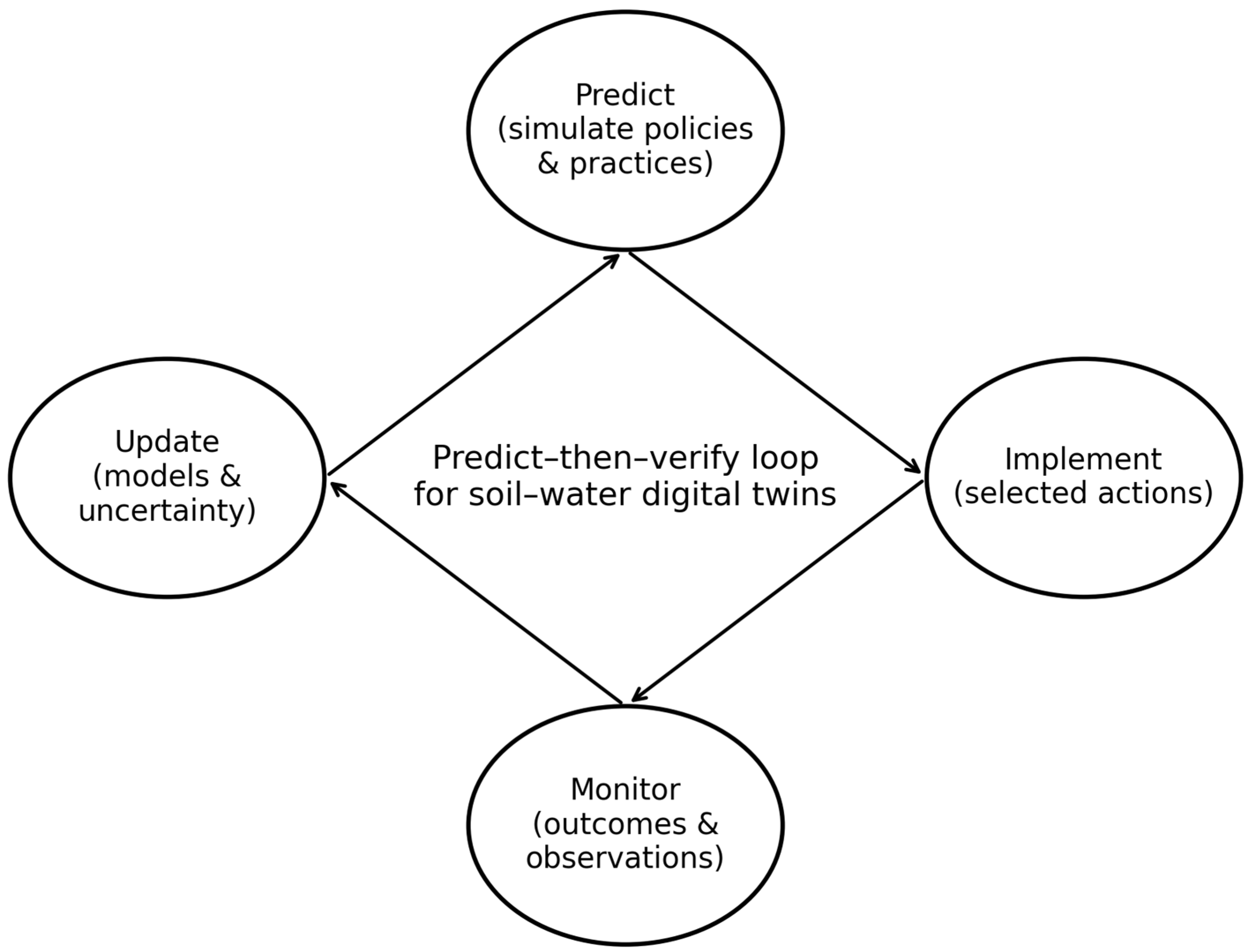
The notion of a “digital twin” has gained traction in water resources as an aspiration to create a live, virtual replica of a physical system [45,46]. For soil–water systems, a digital twin would integrate high-resolution models with real-time data streams (via assimilation, as discussed) to mirror the state of an agricultural landscape or watershed at any given moment [47]. This concept goes hand-in-hand with a predict-then-verify framework: using the digital twin to test or verify the outcomes of proposed interventions (policies, technologies) before implementing them on the ground (Figure 2). In essence, digital twins enable a simulation-based approach to decision-making, where various “what-if” scenarios can be rapidly evaluated with models that are constantly validated against actual conditions.

A digital twin for an agricultural water system would involve several components: Dynamic Modeling Core. A suite of coupled models representing crops, soil moisture, groundwater, and possibly socioeconomic factors (e.g., farmer decisions). The core simulates the water cycle and crop growth continuously, evolving in time.

Data Assimilation Engine. To update the model state, the twin ingests data such as satellite imagery (ET, soil moisture), weather station inputs, IoT soil sensors, and operational data (e.g., irrigation volumes, well pumpage). The assimilation module corrects deviations so that the model remains in sync with reality.

Interface for Scenario Testing. Users (e.g., water managers, policymakers, farmers) can introduce changes in the twin—such as altering an irrigation schedule, implementing a new conservation policy, or simulating an extreme weather event—and the model will predict the system’s response. The outcomes (e.g., crop yield, water table changes, runoff) can be analyzed to verify if the intervention meets objectives.

Uncertainty and Feedback Awareness. The twin would track uncertainties in predictions (via ensemble simulations or statistical methods) and incorporate feedback loops (for instance, economic feedback where water availability might change farmer behavior in the model).

The predict-then-verify concept aligns closely with the scientific method and adaptive management. Rather than deploying a policy broadly and waiting to see results (which can be costly or irreversible if wrong), management can be adaptive: try it in the model, verify if it likely achieves the goals under various conditions, then implement on the ground, and finally use new data to verify outcomes and refine the model. This cycle of prediction and verification is continuous.

Operational and near-operational “twin-like” systems already exist in parts of the soil–water domain, including land data assimilation systems used for drought monitoring and seasonal outlooks, remote-sensing-based ET services that inform irrigation advisory programs, and managed aquifer recharge pilots that combine monitoring networks with scenario modeling. These implementations demonstrate that the digital-twin concept is not purely aspirational, but can be realized incrementally by prioritizing observation operators, uncertainty-aware forecasts, and decision interfaces that match institutional capacity [45,46,47,48,49,50]. Well-established land data assimilation frameworks (e.g., LIS/GLDAS/NLDAS-type systems) illustrate how standardized observation operators and error models can support routine monitoring in regions with sparse ground data [51,52,53].

China’s High-Standard Farmland Construction (HSFC) initiative (a nationwide program to modernize irrigation, land leveling, and soil quality) could benefit from a digital twin approach [36]. A digital twin of a high-standard farmland region might allow planners to verify how proposed infrastructure upgrades would impact soil moisture, yields, and even carbon emissions. The model can be fed with before-and-after data from pilot sites to validate its predictions. The EU and other regions have initiated living labs for digital farming and water management, where test farms are instrumented and modeled in real-time. In California and elsewhere, plans for managed aquifer recharge during wet years (to bank water for droughts) are being evaluated with integrated surface–groundwater models. A digital twin of a groundwater basin, constantly updated with piezometric data and land use changes, can simulate various recharge and pumping patterns to verify if they would stabilize groundwater levels over decades. Only those plans that succeed virtually (with uncertainties accounted for) would be recommended for actual implementation.

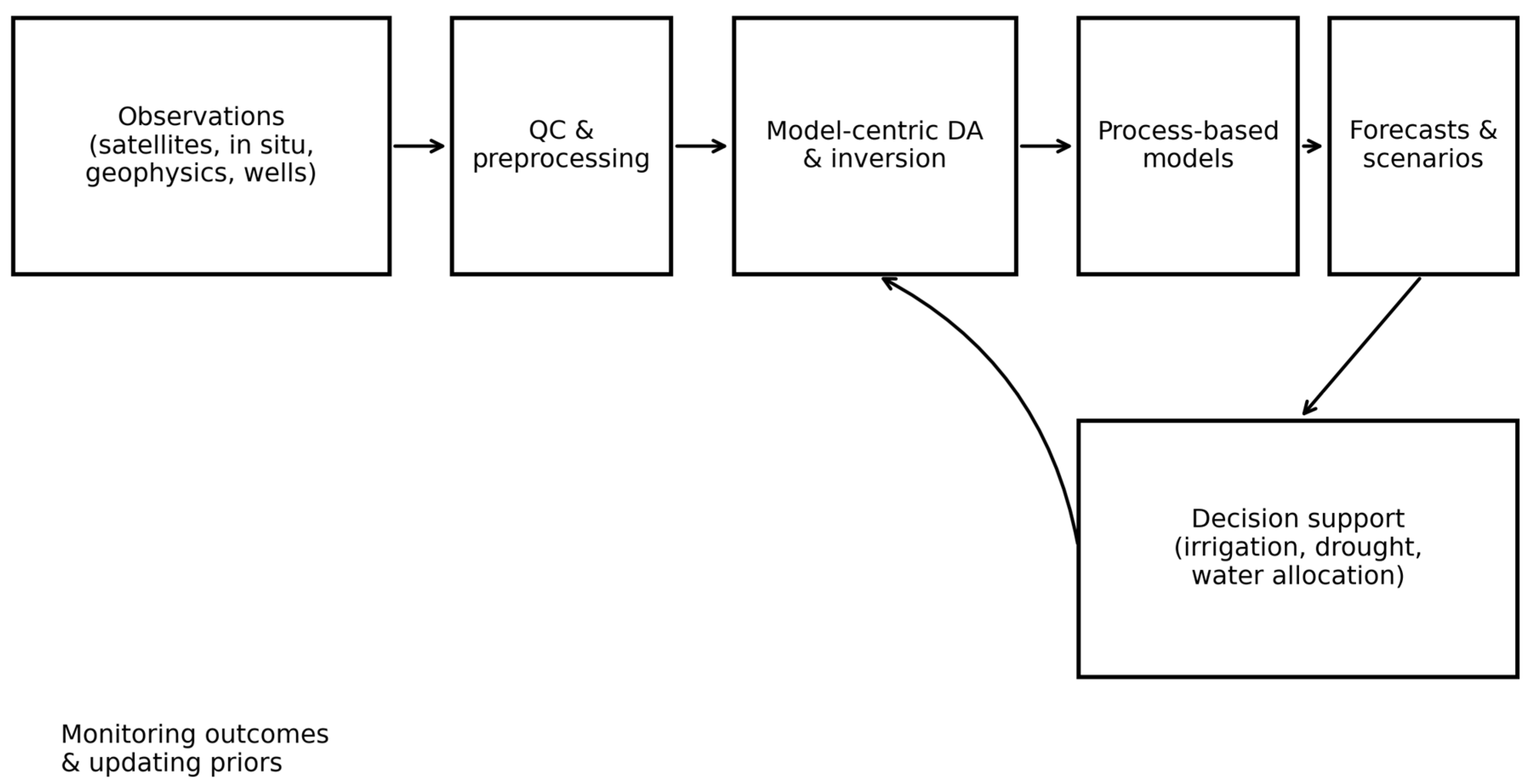
Binley et al. [15] argued for a tighter integration of predictive modeling with field experiments, essentially a closed-loop science wherein models predict outcomes, experiments (or observations) verify them, and discrepancies feed back to improve the models. In the context of soil and water, this is exactly the digital twin paradigm (Figure 3). By continuously reconciling model predictions with multi-scale observations (e.g., using hydrogeophysical surveys to verify model-inferred subsurface moisture patterns [16]), confidence in the model twin grows. Then, when an untested scenario is simulated (such as a future climate or a new irrigation technology), stakeholders can have higher trust in the result.

Advantages: Digital-twin–enabled predict-then-verify management reduces risk by stress-testing policies (e.g., new irrigation scheduling rules) in silico before deployment, revealing unintended impacts such as salinity buildup or yield penalties [47]. Because the twin couples crop–soil–groundwater (and potentially economic) components, it supports holistic evaluation of trade-offs across multiple objectives—water savings, productivity, profitability, and equity of distribution—rather than optimizing a single metric. Scenario visualizations (e.g., maps comparing future groundwater drawdown with and without conservation measures) can strengthen stakeholder engagement and help communicate the rationale for difficult decisions. As new observations arrive (e.g., drought sequences, management changes, or new crop varieties), the twin can be updated and strategies re-verified, enabling adaptive rather than static management [50].

Challenges: Building and maintaining digital twins requires sustained data infrastructure, model-integration expertise, interoperability across heterogeneous data streams, rigorous quality control, and significant computational resources. Because models are inherently imperfect, verification should include independent validation and, for high-stakes interventions, targeted field trials—not reliance on model outputs alone [54]. Scalability is another barrier: a detailed twin may be feasible for a district but prohibitive nationally. A practical solution is multi-scale design—develop high-fidelity twins for representative pilot areas and use reduced-order or AI surrogate models trained on those simulations to extend insights to larger regions.

In conclusion, digital twins represent the convergence of advanced modeling, data assimilation, and adaptive management philosophy. They operationalize the predict-then-verify approach, allowing sustainable soil–water management strategies to be honed and vetted in silico. As data streams (e.g., from remote sensing, IoT sensors) continue to expand and computing capabilities grow, the vision of reliable digital twins for critical water/agriculture regions becomes increasingly attainable [7]. The next sections of this review will explore other cutting-edge methods—tracer and isotope techniques, and agent-based socio-hydrological models—which can enrich models (including digital twins) by providing deeper process insights and representation of human feedback.

6. Tracer-Aided and Isotope Techniques

Water in the soil–plant–atmosphere system is not all the same: it can have different sources, ages, and pathways. Tracer techniques, especially using stable isotopes of hydrogen and oxygen, have become invaluable for disentangling these processes. By “tagging” water molecules, isotopes help partition ET into its components (soil evaporation vs. plant transpiration), identify percolation thresholds in soils, and reveal connectivity between rainfall, soil moisture, and groundwater. Incorporating tracer information into models (so-called tracer-aided modeling) greatly enhances our understanding and predictive capability of soil–water systems.

6.1. Stable Isotopes as Tracers

Oxygen-18 (¹⁸O) and deuterium (²H) are the most commonly used stable isotopes in water. They are ideal tracers because their concentrations in water are modified by phase changes and transport processes in known ways (fractionation). Sprenger et al. [55] note that these isotopes are widely used to track water movement through the soil–plant atmosphere continuum and to separate evaporation from transpiration. How does this work? During evaporation from soil, the lighter isotopes preferentially escape, leaving the remaining soil water enriched in heavy isotopes (¹⁸O and ²H). Transpiration, on the other hand, is often considered not to fractionate isotopes significantly (plants take up water roughly conservatively), though there are nuances. By measuring the isotope ratios in different reservoirs—e.g., soil water at various depths, xylem water in plants, and atmospheric vapor—one can infer what fraction of ET was evaporation vs. transpiration. This is because evaporated water typically has a distinct isotopic signature (often enriched in heavy isotopes and exhibiting lower deuterium-excess) compared to transpired water, which retains the source signature of the soil water. For example, in an experiment, if the surface soil shows isotope enrichment on a hot day while xylem water in plants matches deeper soil water, it indicates that transpiration (from deeper roots) dominates ET, with only a smaller portion coming from evaporation at the surface.

Sprenger et al. [56] conducted tracer studies that revealed evaporation-induced isotopic fractionation can penetrate surprisingly deep into the soil under certain conditions. Their review showed that in arid climates, evaporation signals (enrichment of heavy isotopes) could be found several tens of centimeters down, indicating substantial evaporation flux even from sub-surface layers [55]. This has implications for modeling: a model must allow evaporation not just from the very top layer but possibly from within the profile if dry conditions prevail. Isotope data can thus verify if a model’s evaporation parameterization is realistic. Penna et al. [57] likewise highlighted challenges and opportunities in using stable isotopes for ecohydrology, calling for improved methods to capture spatial and temporal dynamics of isotope signals in soils. They advocated for more continuous in situ monitoring of soil water isotopes (e.g., using new laser spectroscopy techniques and membrane samplers) to move beyond the traditional “snapshot” sampling that misses temporal variability [57]. The development of field-deployable isotopic monitors (vapor probes, continuous analyzers) is now allowing tracer data to be collected at high frequency, which can be fed into models or used to validate their internal flux calculations.

6.2. Partitioning Evaporation vs. Transpiration

A fundamental question for water management is how much of the water loss from land is productive (transpiration that grows crops) versus non-productive (soil evaporation). Stable isotopes provide one of the few ways to quantify this partition at ecosystem scale. For instance, using the isotope mass balance of atmospheric vapor above a canopy (coupled with eddy covariance measurements of ET) can yield transpiration fractions. Many studies have found that transpiration often accounts for ~70–90% of total ET in well-vegetated ecosystems, but in sparse or row-crop agriculture, soil evaporation can be a large component, especially early in the season or under certain tillage practices. Tracer-aided models include isotope modules that simulate fractionation during evaporation and can output isotope ratios of different water pools. By comparing those outputs with measured isotope data (in soil, xylem, etc.), the model’s ET partitioning can be constrained. This approach has been used in experimental plots and catchments (e.g., in Critical Zone Observatory studies) to ensure that models get the “right answer for the right reason”—not just matching total ET but also correctly simulating the split between E and T. For example, a model without tracers might get the total ET correct but do so by overestimating transpiration and underestimating evaporation (or vice versa). Such a model might not perform well under changed conditions (like a shift in crop cover or mulching). Isotope constraints help avoid these compensating errors [56].

6.3. Percolation Thresholds and Transit Times

Tracers are also invaluable for understanding deep percolation (groundwater recharge) and water storage in soils. In many regions, only a fraction of rainfall becomes groundwater recharge—often a threshold exists where the soil has to be sufficiently wet to allow drainage beyond the root zone. By analyzing the isotope signatures of soil water and groundwater over time, one can infer which rainfall events contribute to recharge. For instance, in Mediterranean climates, the first rains after a dry summer may mostly wet up the soil profile (with evaporation fractionation signals observed) but not contribute to groundwater until cumulative wetting overcomes the soil’s storage deficit. At that point, a distinct isotope “pulse” might appear in groundwater wells or stream baseflow. Tracer-aided models can capture this by including dual storage–discharge mechanisms (e.g., mobile vs. less mobile water pools). Isotope evidence [58] spurred debate by showing plant xylem water often had different isotope ratios than stream water, implying ecohydrological separation of water sources. Subsequent work [59] has been refining our understanding of this: how much of that observation is a sampling artifact vs. true separation. Tracer-aided models may consider that only a portion of soil water (often in larger pores) is mobile and contributes to aquifer recharge, whereas water held in micropores might cycle tightly within the root zone.

6.4. Practical Applications of Tracer Information

Partitioning ET helps identify water-saving opportunities. If a significant fraction of irrigation is lost to soil evaporation, practices like mulching or drip irrigation can be justified and their impact quantified. For example, isotope studies might show that in a rice paddy, 30% of water is evaporating directly—a model can then verify that using intermittent drying (alternate wetting and drying) reduces that evaporation fraction, saving water while maintaining yield [5,6].

Tracers also aid in model validation. A hydrologic model might be calibrated against streamflow alone, but if it can also predict isotope dynamics in the stream, that greatly increases confidence that the internal flux partitioning is correct. Some models like STANFORD (an isotope-enabled Topmodel) or the EcH_2O model incorporate isotope simulation and have been tested in headwater catchments where high-frequency rain and runoff isotope data exist. They demonstrated improved identification of parameters like soil depth and preferential flow fractions by matching both flow and isotope signals [55].

6.5. Isotopes of Other Elements and Geochemical Tracers

While H and O isotopes track the water molecule itself, other tracers (chemical or isotopic) can trace solutes and thus water pathways. For example, in soil–groundwater systems subject to fertilizer application, nitrate isotopes (¹⁵N in NO₃) can reveal if water reaching groundwater is coming from quick flow paths or longer residence times (due to isotopic effects of denitrification which occurs over time). Chloride concentration is a classic simple tracer to estimate recharge—measuring chloride accumulation in soil and its dilution during leaching events indicates how much percolation has occurred. Strontium isotopes or trace metals can distinguish water sources (e.g., different geological layers contributing baseflow).

6.6. Isotope Constraints on Model Uncertainty

Including isotope simulation in models provides additional degrees of freedom to constrain uncertain parameters. For example, the timing of an isotopic response in a spring after a rain gives clues about soil drainage rates and preferential flow—parameters that might otherwise be tuned arbitrarily can be narrowed down. Sprenger et al. [59] demonstrated in a forested catchment that models incorporating isotope data could better constrain the soil hydraulic parameters and the proportion of event vs. pre-event water in stormflow, leading to improved predictions of both water quantity and quality (since older water might carry different nutrient loads).

From a practical standpoint, obtaining isotopic data has become easier with laser spectroscopy and lower-cost analysis, but it still requires effort. Hence, tracer-aided modeling is often done in research catchments or pilot studies. The insights gained, however, are broadly useful and can be incorporated into simpler models elsewhere (e.g., knowing typical transpiration fractions for certain crop types can inform large-scale water resource models even without onsite isotope data).

The incorporation of tracers into data assimilation is a frontier area—for example, assimilating vapor isotope measurements (from satellites or ground-based FTIR instruments) into land surface models to adjust evaporation/transpiration partitioning in real time. This is complex (it requires the model to simulate isotopes and treat them as additional state variables in the DA scheme), but initial attempts are being made.

In summary, tracer and isotope techniques shine a unique light on the inner workings of soil–water systems, breaking the “black box” of ET and recharge into understandable components. By integrating these techniques into modeling—through tracer-aided model structures or through validation and calibration—we achieve a more nuanced and reliable representation of processes like evaporation vs. transpiration partitioning and thresholds for deep percolation. These insights ultimately translate to better management: for instance, maximizing transpiration (productive water use) while minimizing unnecessary evaporation, or identifying when soils have replenished sufficiently to generate runoff or recharge, which informs irrigation scheduling and flood control. The Section 7 will shift focus to human dimensions: how models can include human agents, such as farmers, whose decisions critically impact soil and water outcomes.

7. Agent-Based and Socio-Hydrological Models

Water management in agricultural landscapes is fundamentally a human endeavor—farmers decide when and how much to irrigate, what crops to plant, whether to adopt conservation practices, etc. These decisions collectively shape the soil–water system, sometimes in unpredictable ways. Socio-hydrological models seek to represent the two-way interactions between human behavior and hydrology. Within this domain, agent-based models (ABM) have become a popular approach to simulate individual decision-makers (agents) and their collective impact on water resources [54]. This section discusses agent-based and socio-hydrological modeling in the context of sustainable soil–water systems, highlighting how they capture feedback loops such as farmer responses to water availability and the emergent outcomes on resource use.

7.1. Socio-Hydrology and Feedbacks

Traditional hydrological models often treat human influences as external forcing or static inputs (e.g., a fixed pumping rate or a prescribed irrigation schedule). In reality, human behavior responds dynamically to the state of the water system, creating feedback. For instance, if groundwater levels drop, farmers might drill deeper wells or switch crops, which in turn affects the water system further. Socio-hydrology is the study of these coupled dynamics [9]. A classic example is the irrigation paradox—improving irrigation efficiency could lead to expansion of irrigated area by farmers, potentially negating water savings (a rebound effect). Models that ignore this behavioral feedback might overestimate the water saved by a new technology. Socio-hydrological models incorporate relationships such as how farmers’ water use decisions are influenced by water availability, policy incentives, or cultural norms, and conversely how those decisions alter hydrologic variables like river flow or aquifer storage.

7.2. Agent-Based Modeling (ABM)

ABM is a natural tool for socio-hydrology because it simulates many individual actors (agents), each with their own decision rules and interactions [54]. In agricultural water contexts, agents are often farmers or farming households. Each farmer agent may have attributes (farm size, crop type, access to capital, risk preference) and makes decisions (e.g., how much to irrigate, whether to invest in a new irrigation system, whether to participate in a water trading scheme) based on certain rules or behavioral models. These decisions feed into a biophysical model of water flow—for example, the total irrigation withdrawals by all agents determine groundwater pumping volumes, which a groundwater model then uses to update aquifer levels. The new aquifer levels might feed back into agents’ decisions next time (if wells go dry, farmers might reduce planting, etc.). Through many time steps, ABM can simulate emergent patterns like the decline of a groundwater resource under different policy regimes, or the formation of cooperative sharing agreements among farmers.

A recent development is large-scale agent-based hydrological models that simulate not just a handful of farmers but thousands or even millions. de Bruijn et al. [54] introduced the GEB model (Geographical, Environmental, Behavioral), which simulates over 10 million individual farm households in the Krishna River basin in India. This coupled ABM–hydrology model allows each agent to autonomously decide on actions like irrigation, crop selection, and infrastructure investment, while a distributed hydrological model (e.g., the CWatM model) calculates water fluxes and availability on a daily basis. The result is a powerful framework to explore how micro-level adaptations (each farmer’s response to water policies or climate) accumulate into macro-level outcomes (like basin-wide water savings or shifts in cropping patterns). The authors highlight how important it is to consider heterogeneous behavior: some farmers may adopt efficient irrigation, others may not, and these decisions are influenced by social networks and government actions [54]. By explicitly modeling such heterogeneity, ABM can identify conditions under which certain policies succeed or fail. For example, a simulation might show that only if at least 60% of farmers adopt drip irrigation (perhaps encouraged by subsidies and neighbor influence) will the aquifer level stabilize; below that threshold, continued pumping by the remainder still depletes the resource.

7.3. Modeling Farmer Behavior

A key aspect of ABM is how to model decision-making. Approaches range from simple heuristic rules (e.g., “if water table is below X, plant less rice next season”) to more complex economic optimization (each farmer maximizing profit given water constraints) or even bounded rationality and social influence (e.g., agents use imitative behavior or follow norms). An example rule in an irrigation ABM: each farmer decides to irrigate a field if the soil moisture falls below a certain trigger (say 50% depletion) and if they still have water allocation left; otherwise, they let the crop stress. Or in a canal irrigation system modeled by ABM, agents might decide whether to cooperate or defect in water rotation schedules—and the model can simulate the emergence of conflicts or cooperation in water user associations [54]. Some ABMs incorporate learning, where agents adjust their strategies over time based on past outcomes (reinforcement learning) or anticipate future conditions (adaptive expectations).

7.4. Socio-Hydrological Phenomena

With socio-hydrological ABM, one can investigate phenomena such as: Groundwater Tragedy of the Commons. Many farmers pumping from the same aquifer can lead to over-extraction. ABM can test interventions like pumping quotas, water markets, or community management. For instance, an ABM of an aquifer might show that without coordination, agents extract until wells dry (the classic tragedy), but introducing a modest withdrawal fee or a shared quota can significantly extend the aquifer lifespan by altering agent decisions.

Technology Adoption. Why might farmers not adopt a water-saving technology even if it’s beneficial? ABM can include factors like upfront cost, risk aversion, or lack of knowledge. The model can verify under what conditions (e.g., providing subsidies or demonstration projects) adoption becomes widespread enough to have a hydrological impact.

Resilience and Adaptation. ABMs have been used to simulate how farming communities respond to droughts or floods. Some farmers might diversify crops or invest in water storage (ponds), others might exit farming. The socio-hydrological outcomes (like how quickly groundwater recovers after a drought) depend on this distribution of strategies. In one study, an ABM showed that when farmers predominantly grew high-water-demand cash crops, the system was very vulnerable to drought (massive groundwater depletion and crop failures). But if even 30% of the area was kept in low-water-use crops (due to some agents being more risk-averse), the overall system had much less severe groundwater declines. This kind of emergent insight is hard to get from aggregated models.

7.5. Integration with Physical Models

Agent decisions need to translate into model forcings. This often means coupling ABM with hydrological models. There are different coupling schemes: One-way coupling. For example, run a crop water model that calculates yields given water use, feed that as context into an ABM that then decides next year’s planting (like if yield was bad due to water stress, the agent might change behavior). This might not iterate within the year.

Dynamic coupling. The ABM and hydrology run in tandem each time step. For example, on a daily time step: each agent decides pumping for that day, the groundwater model updates heads, then next day, agents see the new head and respond, etc. This can capture rapid feedback.

Networks and Institutions. Some ABMs include social networks or water institutions. For example, if a water users’ association sets a rule (e.g., rotating irrigation turns), the ABM might model compliance—some agents follow, some cheat—and how that affects water distribution and subsequent trust in institutions. This adds another layer beyond just biophysical feedback.

In practice, these couplings are most useful when they explicitly represent decision-making under uncertainty (e.g., incomplete information about aquifer storage, uncertain seasonal rainfall, or unknown policy enforcement) [60]. Recent socio-hydrological work argues for combining behavioral models with probabilistic hydrologic forecasts, so that agents respond to distributions of outcomes (risk) rather than to a single deterministic prediction. This creates a natural role for data assimilation: by reducing forecast uncertainty and updating beliefs about system state, DA can change the incentives and choices simulated by the ABM, enabling more realistic evaluation of policies such as pumping caps, tiered pricing, or drought-triggered restrictions [61,62,63,64].

7.6. Benefits of Including Human Behavior in Models

By explicitly simulating humans, models can predict not just the direct hydrologic outcomes of a management action, but also how people might react and thereby alter those outcomes. For instance, implementing a policy of water quotas could theoretically reduce usage, but if the ABM shows many farmers drill illegal wells to circumvent quotas, the actual reduction might be much smaller [23]. This information is crucial for designing realistic interventions. Agent-based models also allow exploring social dilemmas and cooperation—e.g., under what community sizes or arrangements do farmers willingly self-regulate water use? They can thus inform the design of institutions and governance structures for water.

7.7. Challenges in Socio-Hydrological Modeling

Agent-based socio-hydrological models are complex. Calibrating or validating them is challenging because they have both hydrologic parameters and human behavior parameters. Often there is a lack of data on the latter (surveys, interviews, etc., are needed to formulate the decision rules). There is also significant uncertainty in behavioral rules—humans are not always rational or consistent. Therefore, ABM results are usually analyzed in a scenario or exploratory sense rather than as precise predictions. Computationally, a large ABM with many agents coupled to physical models can be demanding, but advances in computing and more efficient algorithms (and use of cloud or HPC resources) are mitigating this.

Another issue is scale: does one simulate each individual farmer or aggregate them into representative agents? Too much aggregation can wash out the heterogeneity that’s key to emergent phenomena, but too fine detail can be impractical or unnecessary if many agents behave similarly.

Despite these challenges, agent-based and socio-hydrological models are invaluable for addressing the “people aspect” of sustainable soil–water systems. They complement physical models and data assimilation by providing insight into likely human responses to interventions, thereby helping avoid policy pitfalls and ensuring that proposed solutions are robust not just in theory but in practice when human behavior is accounted for.

In summary, incorporating agents (farmers, regulators, water users) into soil–water models allow us to simulate coupled human–water dynamics such as how incentives or social norms influence water use and how water scarcity in turn influences behavior. This is critical for designing management strategies that are both sustainable and socially feasible. The case studies in the Section 8 illustrate some real-world applications where many of the concepts discussed (model coupling, data assimilation, tracer use, socio-hydrology) come together to inform soil–water management across diverse contexts.

8. Case Studies

To ground the concepts discussed so far, we examine several case studies from different climatic and agricultural contexts. These examples highlight how data assimilation and modeling have been applied (or could be applied) for sustainable soil–water management, and what insights have been gained in each context. We focus on: (1) HSFC in China, (2) farms and irrigation management in the United States, (3) the Indo-Gangetic Plain in South Asia, and (4) other illustrative cases (e.g., smallholder farms in Africa or European agroecosystems). Each case demonstrates a unique combination of challenges and modeling solutions.

8.1. China—High-Standard Farmland Construction (HSFC)

China has undertaken a massive campaign to upgrade its agricultural lands under the HSFC program. The goals are to improve irrigation efficiency, soil quality, and infrastructure to boost productivity and resource sustainability [36]. For example, HSFC projects involve leveling fields, lining irrigation canals, building drainage systems, and adopting precision irrigation and fertilization technologies. A study on HSFC impacts noted that it significantly improved soil water retention and fertilizer use efficiency, thereby helping to reduce water and chemical inputs while maintaining yields [36]. Modeling and data assimilation play roles in both planning and evaluating HSFC.

Before implementation, hydrologic models (like SWAT or MODFLOW) have been used to simulate how improved canals or on-farm reservoirs would change water balances. In North China’s plain, where groundwater over-extraction for irrigation has been severe, models predicted that HSFC measures (such as canal lining and introducing sprinklers) could reduce non-beneficial evaporation and seepage losses by up to 30%, translating to measurable groundwater recharge benefits. These predictions are now being verified with field data: satellite measurements show increased green vegetation cover and possibly reduced evaporative fraction after HSFC in some pilot counties. Data assimilation of satellite ET (e.g., using MODIS or newer Gaofen satellite data) has been employed to monitor changes in consumptive water use post-HSFC implementation.

In a critical-zone context, Wang et al. [64] observed that in the Loess Plateau of China, intensive agricultural expansion and land-use shifts led to a significant decline in soil moisture in the critical zone, beyond what climate change alone would predict. This indicates that human land management has been a dominant driver of drying in that region’s soils. Models that included those land-use changes (converting natural vegetation to cropland or terraced fields) reproduced the soil moisture decline better than climate-only scenarios [64]. This case underscores that sustainable management (like HSFC or ecological restoration) is needed to reverse or halt such trends. Going forward, a digital twin of a typical HSFC area could assimilate continuous data (soil moisture from upcoming satellite missions, ET from thermal sensors) to provide feedback on how effective the improvements are and advise if additional measures are needed. For example, if despite HSFC upgrades the soil moisture is still dropping, further changes in crop mix or irrigation practice might be recommended. The HSFC case is essentially a massive real-world experiment where modeling and assimilation inform policy: they help quantify how interventions at field scale add up to regional impacts on water resources and even carbon footprint.

8.2. United States—Farms and Precision Irrigation

In the United States, especially in Western states, water scarcity has driven adoption of precision agriculture and advanced irrigation scheduling. Many farms now use soil moisture sensors and weather-based tools (often via mobile apps or extension services) to decide when to irrigate. Models ranging from simple “checkbook” water budget spreadsheets to complex models like DSSAT or MOHID Land are used to support these decisions.

A case in California’s Central Valley: researchers created a system that combined remotely sensed ET (from satellite thermal imagery) with a crop growth model through data assimilation [65]. This approach provided field-scale estimates of actual crop water use and soil moisture status. By feeding these into a decision support system, farmers received weekly recommendations on irrigation amounts, which in trials, maintained yields with ~15% less water. The assimilation of satellite ET was key because it adjusted the model to reflect the actual crop performance in each field, capturing variability due to factors like soil differences or microclimate that a generic model might miss [65].

Another example is the Ogallala Aquifer region (Great Plains), where declining groundwater is a major concern. Agent-based models have been explored here to simulate how farmers might respond to policies like allocation caps or subsidies for water-saving technology. In one Kansas study, an ABM coupled to an aquifer model suggested that without any intervention, many wells would become non-viable in 2–3 decades. However, if even 20% of farmers switched to drought-tolerant crops and deficit irrigation (possibly incentivized by policy), the aquifer’s lifespan could extend by a decade or more, and the economic output would stabilize rather than collapse. This informed the state’s water planning to encourage crop diversification and to establish “Local Enhanced Management Areas” where collective pumping limits are set (a sort of self-regulation by communities). Models helped verify that if farmers cooperatively reduce pumping by, say, 15%, the long-term benefits (in terms of water availability and farm income) outweigh the short-term production loss.

In terms of assimilation in U.S. operations, systems like NASA’s GRACE-DA for groundwater and the North American Land Data Assimilation System (NLDAS) are used in drought monitoring. These provide soil moisture and groundwater anomaly estimates which regional water managers consult. At the farm scale, a tool called OpenET (developed by a consortium including NASA and others) provides satellite-based ET data to farmers. While not a full assimilation system per se, it is the kind of data stream that can feed models or be directly used for decisions. In an alfalfa field trial, OpenET data was used to adjust a crop model’s forecast of irrigation needs, which improved water use efficiency by preventing over-irrigation during cool periods.

8.3. Indo-Gangetic Plain (South Asia)

The Indo-Gangetic Plain (IGP) is one of the world’s most intensely farmed regions, stretching across Northern India, Pakistan, Nepal, and Bangladesh. It is a breadbasket with rice–wheat rotations and heavy groundwater use, especially in India and Pakistan. Challenges here include groundwater depletion in some areas (e.g., Punjab, Haryana in India), waterlogging and salinity in others, and generally the need to improve water productivity. Modeling and assimilation in this region have been applied at large scales due to its vastness. For instance, researchers in India have used remote sensing-based models (like SWAT and VIC with assimilation) to estimate consumptive water use and available water. They found that in Northwestern IGP, current pumping rates exceed recharge by a large margin, confirming satellite GRACE findings of rapidly declining groundwater storage [17]. These macro-scale models have informed government agencies about the urgency of shifting cropping patterns (like encouraging less rice and more maize or pulses in Punjab) to save water.

One specific effort is the Agricultural Model Intercomparison and Improvement Project (AgMIP) for South Asia, which has applied crop models linked with climate and water models to project the future of IGP agriculture. They incorporate socio-economic scenarios (like demand and prices) too. Such integrated assessments indicated that without adaptation, yields will suffer due to climate change and groundwater depletion by mid-century. However, adaptation options like shifting planting dates, introducing water-saving irrigation, or switching crops can substantially mitigate these effects. For example, replacing flood irrigation of rice with intermittent irrigation and direct-seeding was shown in models to cut water use by ~25% while reducing yield by <5%. Assimilating field trial data on yields and soil moisture back into the models improved their accuracy and gave policymakers more confidence in recommending these practices.

Another initiative is Underground Transfer of Floods for Irrigation (UTFI) in parts of the IGP, where monsoon floodwater is intentionally recharged into aquifers for use in the dry season. Models (MODFLOW and others) combined with on-ground experiments in Uttar Pradesh have been used to verify this strategy. The models predict improved groundwater levels and reduced flood damage, and initial data from pilot sites confirm increased post-monsoon water tables by a few meters. This is an example of a managed aquifer recharge policy being tested with predict-then-verify: model simulations supported the feasibility, and ongoing monitoring (via wells and possibly distributed sensors) is verifying and refining those predictions.

8.4. Other Examples

Sub-Saharan Africa Smallholders: In parts of Africa, data is often scarce, but modeling and assimilation are used in initiatives like TAHMO (Trans-African Hydro-Meteorological Observatory) to maximize the value of limited observations. For instance, in Zambia, an ensemble crop model with remote sensing assimilation was used to estimate soil moisture and yield in farmers’ fields to guide supplemental irrigation from small reservoirs. The assimilation of freely available Sentinel-2 imagery (to update leaf area index in the model) improved yield forecasts. This helps target irrigation only to fields in need, a boon for small-scale schemes with limited water.

To make such applications operational in data-scarce settings, programs increasingly rely on open satellite and reanalysis inputs (precipitation, ET, and soil moisture proxies) combined with land data assimilation systems that provide gridded water-balance states for food and water security monitoring. Examples include drought early-warning workflows that combine CHIRPS-type rainfall estimates with land surface modeling/assimilation, and regional land data assimilation deployments for Sub-Saharan Africa that support famine early warning and irrigation planning [66,67,68,69].

Europe—Precision Irrigation in Spain: Spain’s Segura basin is arid but intensive in fruit and vegetable production. An integrated model assimilating satellite soil moisture (from SMOS) and local sensor networks helped create an irrigation advisory system for farmers. They found that in many cases, farmers were overwatering by ~10%, and by following the model’s recommendations (updated via assimilation to reflect actual soil moisture), they saved water and energy without yield loss. This case underscores how even in advanced agricultural settings, model-data tools can fine-tune practices for greater sustainability.

Latin America and other rapidly irrigating regions face similar challenges of sparse monitoring and competing water demands. Here, remotely sensed ET and vegetation indices are increasingly used to estimate consumptive use and to support enforcement of water allocations, while coupled surface–groundwater models help evaluate trade-offs between short-term production and long-term aquifer depletion. Such approaches are particularly valuable where institutional capacity limits dense in situ networks, making scalable observation-model integration essential for water management [70,71,72,73].

Across all these case studies, some common threads emerge: (1) Integration is key—linking crop, soil, and water models (and sometimes socio-economic elements) provides a more complete picture. (2) Data assimilation and remote sensing greatly enhance model relevance by keeping models tied to reality and extending insights to data-sparse areas. (3) Stakeholder engagement and policy linkage—in each case, model results needed to be translated for decision-makers or farmers. Often, the success of a modeling effort is measured by whether it influenced a policy or practice (like HSFC planning, Kansas water allocations, or Punjab cropping changes). (4) Uncertainty and risk—models are used to explore uncertainties (like climate variability or adoption rates), and scenarios help stakeholders plan in terms of risk management (e.g., preparing for worst-case groundwater decline vs. best-case if conservation is successful).

The case studies show that while challenges differ (from too much water in floods to too little in droughts), the toolkit of modeling, assimilation, tracers, and agent-based approaches can be tailored to each situation. They provide quantitative evidence to support sustainable practices and often reveal counter-intuitive insights (like a small change in behavior can have large effects, or a policy might not work as intended due to human adaptation).

We now turn to an aspect that underpins confidence in all these models—how do we quantify their uncertainty and validate them? This is critical to ensure that model-based recommendations are robust and reliable, which is the focus of the Section 9.

9. Uncertainty Quantification and Model Validation

All models are approximations of reality, and their predictions inherently carry uncertainty [60]. For sustainable soil–water management, quantifying and reducing this uncertainty is crucial—decisions (e.g., how much to restrict irrigation or where to invest in infrastructure) often depend on being reasonably sure of model outcomes. This section discusses sources of uncertainty in soil–water models, methods to quantify and manage uncertainty, and approaches for model validation and skill assessment. Emphasis is given to robust decision-making in the face of uncertainty, aligning with risk-based management principles.

Several factors contribute to uncertainty in model predictions:

Forcing Uncertainty. Uncertainty in inputs like future climate (rainfall, ET) or water demand scenarios. For instance, different climate models may disagree on rainfall trends, which propagates to uncertainty in soil moisture or recharge forecasts.

Parameter Uncertainty. Soil and aquifer parameters (e.g., hydraulic conductivity, field capacity, crop coefficients) are not known with precision. They are often inferred from limited measurements or calibration, leading to ranges of possible values that yield different results.

Structural Uncertainty. No model structure perfectly represents reality. Process simplifications or omissions (e.g., not including macropore flow, or representing groundwater with a linear reservoir instead of a more complex formulation) cause structural error. Montanari and Koutsoyiannis [4] emphasize that even with best efforts, epistemic uncertainty remains because of these model imperfections.

Initial and Boundary Condition Uncertainty. For instance, the initial soil moisture profile or initial groundwater levels might not be well known. Small errors there can influence subsequent model behavior (though data assimilation helps reduce this).

Observation Uncertainty. When validating, the data themselves have error (e.g., satellite soil moisture has measurement error, groundwater level readings might have noise), complicating comparison.

To quantify uncertainty, a common approach is to perform sensitivity analyses and run ensembles of model simulations. For example, to evaluate parameter uncertainty, one can sample parameter sets from distributions (Monte Carlo or Latin Hypercube sampling) and run the model for each set. The spread of outcomes (say, in predicted irrigation water use or aquifer drawdown) provides a measure of uncertainty. Recent work [8] involved a global sensitivity analysis of a land surface model, identifying which uncertain parameters most strongly influence evaporation, transpiration, and recharge outputs. Their analysis showed, for instance, that evaporation was primarily controlled by parameters related to energy transfer (canopy resistance, litter layer properties), while groundwater recharge was sensitive to only a small subset of parameters (like root zone drainage rates). This kind of insight helps prioritize which parameters need better measurement or calibration, effectively reducing uncertainty by focusing efforts. It also helps simplify models—if some parameters hardly affect key outputs, the model complexity can potentially be reduced or those parameters fixed to nominal values.

Another tool is the output of the Kalman filter variance (in assimilation systems)—for example, an ensemble Kalman filter provides error covariance for the state estimates, which can be propagated to forecast uncertainty. For instance, an EnKF might give a confidence interval for soil moisture next week; a decision-maker could use that by, say, scheduling irrigation with a buffer if uncertainty is high (e.g., water a little extra if there is a significant chance the soil might dry more than expected) [74].

Uncertainty Propagation and Scenario Analysis: For forcing uncertainty, scenario analysis is common. Hydrologic models might be run with multiple climate projections (wet scenario, dry scenario, median scenario, etc.) to see a range of possible futures. If all scenarios lead to the same conclusion (e.g., aquifer depletion) then robust evidence action is needed. If they diverge, one might take a precautionary approach or plan to monitor closely and adapt as reality unfolds.

Converting Deterministic Models to Stochastic Predictions: Montanari & Koutsoyiannis [4] proposed a blueprint where deterministic model outputs are post-processed to estimate predictive uncertainty. One method is to treat model error as a stochastic process—for example, use past performance on validation data to infer error distributions and then add that as noise to future predictions. The “two-stage” approach involves (1) running the deterministic model, and (2) using a statistical model of residuals (like a time-series error model) to generate prediction intervals. This has been applied in hydrology for streamflow forecasts, where after simulation one might fit an AR(1) model to residuals or use quantile regression to estimate the 5th and 95th percentile errors as a function of flow or season. In soil moisture prediction, a similar technique could calibrate an uncertainty model such that, say, when soil moisture is very low, the model error might skew in one direction (perhaps models typically underestimate extreme drying, etc.). The outcome is a probabilistic forecast rather than a single deterministic trace.

Validation and Model Skill Assessment: Validation is checking model outputs against independent observations not used in calibration. A robust validation for soil–water models ideally checks multiple variables across scales (for instance, check soil moisture at a few depths, ET against a flux tower, and streamflow or groundwater levels concurrently). A multi-criteria validation gives more confidence than just one metric. For example, a watershed model might be calibrated to streamflow but then validated against remotely sensed soil moisture patterns and groundwater trends. If it matches all reasonably well, it implies the internal partitioning is likely sound. If not, one might identify biases—e.g., perhaps the model gets streamflow right by overestimating baseflow and underestimating quick runoff, which might be revealed by a mismatch in soil moisture or isotope signals. Using tracers and isotopes in validation, as discussed earlier, is a powerful way to check the internal consistency of model fluxes [75]. Furthermore, cross-validation techniques (like split-sample testing or leave-one-out) can gauge model robustness. For instance, calibrate on data from years 1–5 and validate on years 6–10, or calibrate in a wetter period and test in a drought period to see if the model holds up.

Performance Metrics: Common metrics include RMSE (Root Mean Square Error) and NSE (Nash–Sutcliffe Efficiency) for continuous variables like soil moisture or streamflow, and categorical metrics for events (e.g., did the model correctly predict occurrence of a drought or a threshold exceedance). For probabilistic predictions, metrics like CRPS or reliability diagrams are used to assess if predicted probabilities match observed frequencies. In assimilation contexts, innovation statistics (observation minus forecast) are monitored; if the filter is optimal, innovations should be zero-mean and have variance consistent with predicted error. Significant biases or mis-specified variances indicate model or assimilation issues to address.

Model Intercomparison: Sometimes multiple models are run and compared (an ensemble of models rather than just an ensemble of parameters)—this addresses structural uncertainty to an extent. If different reputable models agree, that boosts confidence. Large projects like ISI-MIP or intercomparison studies have compared hydrological models in various basins to assess uncertainty due to model structure. For soil moisture, the GLDAS system compares multiple land surface models (Noah, VIC, Mosaic, etc.)—if they all produce a drought signal, it is robust; if some diverge, one digs into why (different root depth assumptions? different soil parameterizations? etc.).

Reducing Uncertainty: Data assimilation itself is a way of reducing state uncertainty by continually correcting the model with observations. Another approach is adaptive sampling—figuring out what new data would reduce uncertainty the most. For instance, a data-worth analysis might show that installing a cosmic-ray soil moisture sensor in a particular part of a watershed would greatly reduce uncertainty in model predictions of recharge (maybe because that area is a major contributor to recharge and currently unobserved). This can guide monitoring network design. Similarly, if a certain parameter (like deep soil hydraulic conductivity) is causing wide uncertainty in recharge estimates, one might perform targeted field experiments (like borehole permeameter tests) to better constrain it.

Risk-Based Decision Making: In practice, decisions have to be made even with uncertainty. This leads to methods like robust optimization and expected utility. For example, an irrigation district might use the model to project water availability for the season with uncertainty bounds. They could decide on an allocation that is safe under, say, 90% of scenarios (a conservative approach) or plan contingent measures if the worst 10% case happens. Uncertainty quantification allows creation of decision rules like “If predicted river flow has >20% chance of falling below X, start rationing water early”—essentially formalizing precautionary thresholds. For soil–water management, “decision-centric” uncertainty analysis can be strengthened by borrowing tools from robust decision making and adaptive pathways planning. Rather than optimizing for a single assumed future, these approaches evaluate policies over large ensembles of plausible climate, market, and governance scenarios, identifying no-regrets or low-regret actions and revealing tipping points where strategies fail. In digital-twin settings, the value of information framework can further quantify whether adding a new sensor stream (e.g., ET maps or groundwater heads) is worth its cost because it measurably reduces decision uncertainty [76,77,78,79].

Communicating Uncertainty: This is part of model validation in a broader sense—being transparent with stakeholders about how confident we are. Too often, model results are taken as precise, which can backfire if reality deviates. Instead, providing prediction intervals or scenario ranges can prepare users for variability. Visual tools like fan plots (shaded regions showing uncertainty bands over time) or probability maps (e.g., a map of probability that groundwater will fall below a critical threshold) are effective ways to communicate uncertainty.

Continuous Verification: Model validation is not a one-time step; in operational settings, it is continuous. As new data come in (e.g., each season or year), they are used to update and re-validate the model. If a model consistently performs poorly in some aspect, it may need refinement. This is where approaches akin to machine learning can complement—e.g., using residual error patterns to correct model biases (sometimes called bias correction or model output statistics). Montanari & Koutsoyiannis’s approach of turning deterministic outputs into stochastic predictions via error modeling can be viewed as a form of continuous verification and adjustment [4].

In summary, robust modeling for soil–water systems involves acknowledging uncertainties, quantifying them, and actively working to reduce and communicate them. Techniques range from ensemble simulation, sensitivity analysis, and tracer constraints to advanced data assimilation and error modeling. Validation against real-world measurements (including unconventional data like isotopes or farmer-reported outcomes) is the ultimate test of a model’s reliability. By addressing uncertainty head-on, we can shift management discussions from asking “Is the model right or wrong?” to “Given what is likely or unlikely per the model, how do we manage risk?” This mindset is essential in a changing and uncertain future climate. Having covered the breadth of methods and applications—observation systems, modeling frameworks, assimilation, digital twins, tracers, human-in-the-loop models, and uncertainty handling—we now synthesize the best practices and future needs for integrated soil–water modeling, and conclude with an outlook for this critical field.

10. Research Gaps and Future Directions

Despite significant progress in data assimilation and modeling for soil–water systems, many challenges remain. This section outlines key research gaps and potential future directions to further improve integrated soil–water modeling for sustainable management. The focus is on emerging technologies and methodologies that could be game-changers, as well as the need for interdisciplinary integration and real-world implementation.

10.1. Enhanced Sensor Integration and Big Data

One gap is fully exploiting the wealth of new data sources. We have more satellites, drones, and ground sensors than ever, but integrating them seamlessly into models is still an active area of research. For instance, the upcoming NASA–ISRO NISAR mission and the newly launched Surface Water and Ocean Topography (SWOT) mission will provide high-resolution measurements (for soil moisture and water levels in rivers/canals respectively). Integrating such data could improve irrigation district models by providing near-real-time inflow/outflow information. Similarly, the proliferation of IoT soil moisture sensors (cheap capacitance probes, etc.) on farms offers high-frequency, site-specific data. However, these data are often noisy and not standardized. Research is needed on assimilation techniques that can handle unstructured big data—e.g., hundreds of sensor readings coming in asynchronously—perhaps leveraging machine learning to filter and bias-correct them before assimilation. The concept of an “Internet of Water” has been floated, where diverse water data (stream gauges, wells, satellites, weather forecasts) are accessible via cloud platforms to feed digital twins [8]. Realizing this will require not only technical development of APIs and data standards, but also addressing privacy and data-sharing concerns (for example, some farmers may be wary of sharing real-time water use data).

10.2. Scalable Assimilation Algorithms

Many assimilation methods struggle with large, high-resolution models due to computational cost. The development of more efficient algorithms, or better use of parallel/cloud computing, is a key frontier. For example, particle filters that normally require many particles could be combined with machine learning surrogates to focus particles in plausible regions of state space, making them more efficient (early work uses neural networks to emulate parts of the model within a PF loop). Alternatively, hierarchical assimilation—assimilating data first at coarse scales, then downscaling the corrections—might allow tackling high-resolution systems stepwise. As models move toward including millions of agents or very fine grid cells (like a digital twin with 10 m resolution soil grids and thousands of farms), assimilation methods will need to handle state vectors of enormous dimension. Research into reducing dimensionality (via state compression or localization strategies) is ongoing. There is also potential in distributed computing approaches: imagine an assimilation system where each agent (farm) model assimilates its own local data and occasionally synchronizes with neighbors or a central model. This could mimic how real decisions are made (locally) and might be computationally easier than one monolithic assimilation of everything.

10.3. Artificial Intelligence (AI) Integration

AI and machine learning can contribute in multiple ways. Hybrid modeling, where a physical model is supplemented by a machine learning component to capture processes that are hard to quantify, is a promising direction. For example, one could use a neural network to learn the relationship between certain soil sensor patterns and the onset of runoff, or between weather patterns and farmers’ irrigation decisions, and then embed that learned component into a larger model. Another use of AI is in developing emulators—training surrogate models (e.g., Gaussian processes or neural nets) to approximate the outputs of expensive simulations. These emulators can then be used in Monte Carlo uncertainty analysis or optimization much faster than running the full model each time. AI can also assist in pattern recognition: scanning through remote sensing data to identify anomalies (like where crops are water-stressed or where irrigation is occurring outside of policy) and flagging those for modelers or managers. However, a gap is ensuring AI methods respect physical laws—pure black-box models might give unrealistic or non-generalizable results if used blindly. There is a push for “Physics-Informed Machine Learning” (PIML), which constrains AI models with known physics (mass balance, energy conservation, etc.), bridging the gap between pure ML and traditional process modeling. Recent work on theory-guided learning, Earth-system deep learning, and physics-informed neural networks provides a pathway to build fast emulators and differentiable surrogates that can reduce computational cost while respecting conservation laws—potentially enabling real-time DA at management scales [80,81,82,83].

10.4. Towards Real-Time Adaptive Management

Most current model applications are advisory or scenario-based (i.e., they provide recommendations to humans). A future direction is closing the loop: models directly controlling or adjusting management in real-time (with human oversight). For example, an automated irrigation system where a model assimilation of weather and soil data triggers irrigation events in a “smart farm” without waiting for human input. Some advanced greenhouses already do this (models optimize climate and irrigation control), but open-field agriculture could also benefit, especially with the advent of 5G networks and robust field sensors/actuators. Research is needed on reliable automated decision algorithms and fail-safes (to avoid, say, a sensor glitch causing unnecessary irrigation or a dangerous lack of irrigation).

10.5. Equity and Policy Relevance

A gap often not technical but socio-political is ensuring that the benefits of advanced modeling reach all stakeholders, including smallholder and marginalized farmers. There is a risk that high-tech solutions only benefit large, resource-rich operations. Future work should focus on accessibility: creating modeling tools that are user-friendly and affordable, possibly open-source, and that can run on standard PCs or even smartphones (for instance, a simple water balance app powered by data assimilation that a small farmer can use). Capacity building is important: training extension officers and local agronomists in these tools so they can be disseminated. Moreover, models should incorporate metrics of equity—for example, when evaluating a water policy, the model should output not just total economic gain but also distributional impacts: do small farms suffer more than large ones? ABMs can help with this by representing different farm sizes and wealth levels. Including such outputs can guide policies that are more equitable (for instance, by showing that without certain safeguards, a groundwater cap could push small farmers out while large ones cope, leading to greater rural inequity).

10.6. Climate Change and Non-Stationarity

The future will not look like the past, and models must handle non-stationary conditions—new temperature regimes, possibly more intense rainfall or prolonged droughts, etc. Many models’ parameters (like crop coefficients or irrigation requirements) are calibrated on historical observations. As conditions shift (e.g., CO₂ increase affecting transpiration efficiency, or new crop varieties with different water use), these may change. More research is needed on dynamic or adaptive parameterizations. Data assimilation can help by recalibrating models on the fly as new observations come in under changing conditions. But there may also be novel processes (e.g., heat stress beyond historical experience affecting plant water use, or pest outbreaks altering transpiration by defoliation) that models need to incorporate. Thus, continued field research and model development is needed to capture emerging processes under climate change.

10.7. Holistic Coupling of Sectors

Soil–water systems are linked to other sectors like energy (pumping costs, hydropower), ecosystems (biodiversity, pollination), and climate (carbon sequestration in soils, greenhouse gas emissions from wetlands or rice paddies). Future integrated models may need to couple water, food, energy, and ecology models for truly sustainable planning—the so-called Water-Energy-Food (WEF) nexus modeling. For instance, if promoting a shift from flood-irrigated rice to solar-pumped micro-irrigation of orchards, one should model not only water saved but the energy used by pumps and the economic implications. Multisectoral models exist but data assimilation across them is rare. Could we assimilate economic indicators or satellite data on crop types into these broader models? It is an open area for exploration.

10.8. Transdisciplinary Collaboration

Finally, a gap that is being addressed but needs further push is involving end-users in model development. Co-development of models with farmers, water managers, and policymakers can ensure the models address the right questions and their outputs are in a usable form. This is more of a process gap. Techniques like participatory modeling are valuable—for example, using serious games or interactive simulators in workshops where stakeholders can tweak scenarios and immediately see model outputs, thus learning and also guiding model improvement.

Future soil–water management will likely rely on automated, high-resolution model–data fusion systems that operate as real-time decision backbones [71]. Always-on sensor webs will stream into cloud models, while AI-enhanced assimilation will issue actionable alerts—e.g., predicting a field will cross a soil-moisture stress threshold within three days and triggering preemptive irrigation or other measures. Farmers will access these insights through simple mobile dashboards or voice queries that hide complex analytics behind intuitive interfaces.

At regional scales, digital twins will let policymakers virtually test policy portfolios (pricing, regulations, infrastructure) while accounting for coupled human and hydrologic responses. Achieving this vision demands advances in the technical areas above plus sustained efforts to build user trust, transparency, and operational capacity. If successful, soil–water governance can shift from reactive, anecdotal choices to proactive, evidence-based, adaptive strategies that protect both productivity and long-term resource conservation [18,23].

10.9. Data Scarcity and Capacity Building in Low- and Middle-Income Regions

A recurring barrier to actionable soil–water modeling is the limited availability of long, quality-controlled time series of soil hydraulic properties, management practices, pumping records, and groundwater observations—particularly in low-and middle-income regions. Progress therefore depends on strategies that are robust to sparse data: (i) leveraging globally available satellite products and re-analyses as “first-order” constraints; (ii) designing low-cost, scalable monitoring (e.g., community wells, mobile surveys, cosmic-ray neutron rovers); (iii) transferring information across regions via similarity, regionalization, or machine-learning surrogates; and (iv) explicitly quantifying uncertainty so that decisions can be prioritized even when data are incomplete [66,67,68,84,85,86,87].

Equity considerations are not only ethical but also technical: model performance can degrade when algorithms and parameter priors are trained primarily in well-instrumented regions. Community co-design, open data infrastructures, and capacity building are therefore essential components of sustainable digital-twin programs, ensuring that model–data fusion supports locally relevant decisions and does not amplify existing disparities in access to information and water security [88,89,90].

11. Conclusions

Data assimilation and modeling for sustainable soil–water systems have matured into a multidisciplinary toolkit for smarter stewardship of water and soils. This review synthesizes advances from observation to prediction across scales, emphasizing that integration is indispensable: no single model or data stream can represent the coupled crop–vadose–groundwater continuum or its human controls. The most successful studies combine process models (e.g., APSIM, SWAT, HYDRUS, MIKE SHE) and merge ground sensors, remote sensing, hydrogeophysics, and tracers to build a coherent picture of states and fluxes. Data assimilation—especially ensemble Kalman and variational approaches—adds clear value by continuously reconciling simulations with observations, reducing uncertainty, and enabling actionable forecasts (soil moisture, ET, groundwater storage) that underpin digital twins. Tracer and isotope information further constrains internal partitioning (evaporation vs. transpiration, recharge thresholds), limiting equifinality and increasing confidence in predictions under novel conditions. Finally, socio-hydrological and agent-based models remind us that adoption, incentives, and behavioral feedback can amplify or negate technical gains, so sustainable solutions must be evaluated within realistic decision environments.

A recurring lesson is that uncertainty should be embraced, quantified, and communicated—not hidden. Ensemble prediction, sensitivity analysis, and multi-criteria validation enable risk-informed decisions and the shift from deterministic outputs to probabilistic guidance, as advocated in process-based hydrologic modeling. The field is also moving toward continuous improvement through “predict–then–verify” digital-twin workflows: test policies and practices in silico, implement robust options, monitor outcomes, and assimilate new data to update models and refine decisions. Looking forward, tighter coupling of sensing, modeling, and management—supported by scalable computation, interoperable data pipelines, and responsible governance—can enable proactive irrigation and groundwater planning under climate and market volatility. Technology alone will not deliver sustainability; institutional support, stakeholder engagement, and capacity building are equally critical. Taken together, integrated modeling and data assimilation, enriched by tracers and human-behavior representations, provide a pathway from reactive management to adaptive, evidence-based strategies that maintain productivity while conserving soil health and water for future generations.

Key takeaways from the expanded review are: (1) model-centric data assimilation is the practical pathway to fuse multi-source observations with coupled crop–vadose–groundwater models; (2) benchmarking and open, reproducible workflows are needed to compare DA methods fairly and to translate research into operations; (3) digital twins enable a predict-then-verify cycle that reduces risk by stress-testing management actions before implementation; (4) tracer-aided components and socio-hydrological models help resolve “why” changes occur by partitioning fluxes and representing adaptive human behavior; and (5) closing the data and capacity gap in low-and middle-income regions is essential for globally equitable soil–water sustainability.

Future advances will likely come from hybrid architectures that combine mechanistic models with machine-learning emulators, from uncertainty-aware decision analytics (robust/adaptive pathways), and from community platforms that standardize observation operators, error models, and evaluation datasets. Together, these steps can accelerate the development of reliable, decision-ready soil–water digital twins that support sustainable agriculture under climate and socio-economic change.

References

1. World Economic Forum. Global Risks 2015, 10th ed.; World Economic Forum: Geneva, Switzerland, 2015. [Google Scholar]
2. Food and Agriculture Organization of the United Nations. Water for Sustainable Food and Agriculture; FAO: Rome, Italy, 2017. [Google Scholar]
3. He, L.; Rosa, L. Solutions to agricultural green water scarcity under climate change. PNAS Nexus 2023, 2, pgad117. [Google Scholar] [CrossRef]
4. Montanari, A.; Koutsoyiannis, D. A blueprint for process-based modeling of uncertain hydrological systems. Water Resour. Res. 2012, 48, W09555. [Google Scholar] [CrossRef]
5. Clark, M.P.; Nijssen, B.; Lundquist, J.D.; Kavetski, D.; Rupp, D.E.; Woods, R.A.; Freer, J.E.; Gutmann, E.D.; Wood, A.W.; Brekke, L.D.; et al. A unified approach for process-based hydrologic modeling: 1. Modeling concept. Water Resour. Res. 2015, 51, 2498–2514. [Google Scholar] [CrossRef]
6. Clark, M.P.; Nijssen, B.; Lundquist, J.D.; Kavetski, D.; Rupp, D.E.; Woods, R.A.; Freer, J.E.; Gutmann, E.D.; Wood, A.W.; Gochis, D.J.; et al. A unified approach for process-based hydrologic modeling: 2. Model implementation and case studies. Water Resour. Res. 2015, 51, 2515–2532. [Google Scholar] [CrossRef]
7. Huang, L.; Luo, Y.; Chen, J.M.; Tang, Q.; Steenhuis, T.; Cheng, W.; Shi, W. Satellite-based near-real- time global daily terrestrial evapotranspiration estimates. Earth Syst. Sci. Data 2024, 16, 3993–4017. [Google Scholar] [CrossRef]
8. Dell’Oca, A.; Luttenauer, D.; Guadagnini, A.; Weill, S.; Ackerer, P. Relative importance of uncertain model parameters driving water fluxes in a land surface model. J. Hydrol. 2025, 663, 134310. [Google Scholar] [CrossRef]
9. Sivapalan, M.; Savenije, H.H.G.; Blöschl, G. Socio-hydrology: A new science of people and water. Hydrol. Process. 2012, 26, 1270–1276. [Google Scholar] [CrossRef]
10. Miralles, D.G.; Jiménez, C.; Jung, M.; Michel, D.; Ershadi, A.; McCabe, M.F.; Hirschi, M.; Martens, B.; Dolman, A.J.; Fisher, J.B.; et al. The WACMOS-ET project—Part 2: Evaluation of global terrestrial evaporation data sets. Hydrol. Earth Syst. Sci. 2016, 20, 823–842. [Google Scholar] [CrossRef]
11. Allen, R.G.; Tasumi, M.; Trezza, R. Satellite-based energy balance for mapping evapotranspiration with internalized calibration. (METRIC)—Model. J. Irrig. Drain. Eng. 2007, 133, 380–394. [Google Scholar] [CrossRef]
12. Reichle, R.H.; De Lannoy, G.J.M.; Liu, Q.; Ardizzone, J.V.; Colliander, A.; Conaty, A.; Crow, W.; Jackson, T.J.; Jones, L.A.; Kimball, J.S.; et al. Assessment of the SMAP Level-4 Surface and Root- Zone Soil Moisture Product Using In Situ Measurements. J. Hydrometeorol. 2017, 18, 2621–2645. [Google Scholar] [CrossRef]
13. Zreda, M.; Shuttleworth, W.J.; Zeng, X.; Zweck, C.; Desilets, D.; Franz, T.; Rosolem, R. COSMOS: The COsmic-ray Soil Moisture Observing System. Hydrol. Earth Syst. Sci. 2012, 16, 4079–4099. [Google Scholar] [CrossRef]
14. Franz, T.E.; Zreda, M.; Ferre, T.P.A.; Rosolem, R.; Zweck, C.; Stillman, S.; Zeng, X.; Shuttleworth, W.J. Measurement depth of the cosmic ray soil moisture probe affected by hydrogen from various sources. Water Resour. Res. 2012, 48, W08515. [Google Scholar] [CrossRef]
15. Binley, A.; Hubbard, S.S.; Huisman, J.A.; Revil, A.; Robinson, D.A.; Singha, K.; Slater, L.D. The emergence of hydrogeophysics for improved understanding of subsurface processes over multiple scales. Water Resour. Res. 2015, 51, 3837–3866. [Google Scholar] [CrossRef]
16. Allen, R.G.; Pereira, L.S.; Raes, D.; Smith, M. Crop Evapotranspiration—Guidelines for Computing Crop Water Requirements; FAO Irrigation and Drainage Paper 56; FAO: Rome, Italy, 1998. [Google Scholar]
17. MacDonald, A.M.; Bonsor, H.C.; Dochartaigh, B.É.Ó.; Taylor, R.G. Groundwater Resources in the Indo-Gangetic Basin: Resilience to Climate Change and Abstraction; British Geological Survey Open Report OR/15/047; British Geological Survey: Nottingham, UK, 2015. [Google Scholar]
18. Holzworth, D.P.; Huth, N.I.; de Voil, P.G.; Zurcher, E.J.; Herrmann, N.I.; McLean, G.; Chenu, K.; van Oosterom, E.J.; Snow, V.; Murphy, C.; et al. APSIM—Evolution towards a new generation of agricultural systems simulation. Environ. Model. Softw. 2014, 62, 327–350. [Google Scholar] [CrossRef]
19. Liu, X.; Yan, Z.; Shen, Y.-J.; Min, L.; Wang, S.; Shen, Y.; Guo, Y. Quantifying the effects of irrigation schedule on groundwater level variability using a linked APSIM–MODFLOW model framework. Agric. Water Manag. 2025, 316, 109610. [Google Scholar] [CrossRef]
20. Gassman, P.W.; Reyes, M.R.; Green, C.H.; Arnold, J.G. The Soil and Water Assessment Tool: Historical Development, Applications, and Future Research Directions. Trans. ASABE 2007, 50, 1211–1250. [Google Scholar] [CrossRef]
21. Šimůnek, J.; Šejna, M.; Saito, H.; Sakai, M.; van Genuchten, M.T. Recent developments and applications of the HYDRUS computer software packages. Vadose Zone J. 2016, 15, 1–25. [Google Scholar] [CrossRef]
22. Abbott, M.B.; Bathurst, J.C.; Cunge, J.A.; O’Connell, P.E.; Rasmussen, J. An introduction to the European Hydrological System—Système Hydrologique Européen, “SHE”, 1: History and philosophy of a physically-based, distributed modeling system. J. Hydrol. 1986, 87, 45–59. [Google Scholar] [CrossRef]
23. Ma, L.; He, C.; Bian, H.; Sheng, L. MIKE SHE modeling of ecohydrological processes: Merits, applications, and challenges. Ecol. Eng. 2016, 96, 137–149. [Google Scholar] [CrossRef]
24. Jones, J.W.; Hoogenboom, G.; Porter, C.H.; Boote, K.J.; Batchelor, W.D.; Hunt, L.A.; Wilkens, P.W.; Singh, U.; Gijsman, A.J.; Ritchie, J.T. The DSSAT cropping system model. Eur. J. Agron. 2003, 18, 235–265. [Google Scholar] [CrossRef]
25. Steduto, P.; Hsiao, T.C.; Fereres, E.; Raes, D. AquaCrop—The FAO crop model to simulate yield response to water: I. Concepts and underlying principles. Agron. J. 2009, 101, 426–437. [Google Scholar] [CrossRef]
26. Raes, D.; Steduto, P.; Hsiao, T.C.; Fereres, E. AquaCrop—The FAO crop model to simulate yield response to water: II. Main algorithms and software description. Agron. J. 2009, 101, 438–447. [Google Scholar] [CrossRef]
27. Williams, J.R. The EPIC model. In Computer Models of Watershed Hydrology; Singh, V.P., Ed.; Water Resources Publications: Highlands Ranch, CO, USA, 1995; pp. 909–1000. [Google Scholar]
28. Burrough, P.A.; McDonnell, R.A. Principles of Geographical Information Systems; Oxford University Press: Oxford, UK, 1998. [Google Scholar]
29. Mure-Ravaud, M.; Binet, G.; Bracq, M.; Perarnaud, J.-J.; Fradin, A.; Litrico, X. A web based tool for operational real-time flood forecasting using data assimilation to update hydraulic states. Environ. Model. Softw. 2016, 84, 35–49. [Google Scholar] [CrossRef]
30. Jenson, S.K.; Domingue, J.O. Extracting topographic structure from digital elevation data for geographic information system analysis. Photogramm. Eng. Remote Sens. 1988, 54, 1593–1600. [Google Scholar]
31. Tarboton, D.G. A new method for the determination of flow directions and contributing areas in grid digital elevation models. Water Resour. Res. 1997, 33, 309–319. [Google Scholar] [CrossRef]
32. Kalnay, E. Atmospheric Modeling, Data Assimilation and Predictability; Cambridge University Press: Cambridge, UK, 2003. [Google Scholar]
33. Girotto, M.; De Lannoy, G.J.M.; Reichle, R.H.; Rodell, M.; Draper, C.; Bhanja, S.N.; Mukherjee, A. Benefits and pitfalls of GRACE data assimilation: A case study of terrestrial water storage depletion in India. Geophys. Res. Lett. 2017, 44, 4107–4115. [Google Scholar] [CrossRef]
34. Liu, Y.; Weerts, A.H.; Clark, M.; Hendricks Franssen, H.-J.; Kumar, S.; Moradkhani, H.; Seo, D.-J.; Schwanenberg, D.; Smith, P.; van Dijk, A.I.J.M.; et al. Advancing data assimilation in operational hydrologic forecasting: Progresses, challenges, and emerging opportunities. Hydrol. Earth Syst. Sci. 2012, 16, 3863–3887. [Google Scholar] [CrossRef]
35. Beven, K.; Binley, A. The future of distributed models: Model calibration and uncertainty prediction. Hydrol. Process. 1992, 6, 279–298. [Google Scholar] [CrossRef]
36. Ren, F.; Xia, Z.; Huang, Y.; Chi, J.; He, G.; Wang, Y. The impact of high standard farmland construction on China’s agricultural resilience. Sci. Rep. 2025, 15, 38626. [Google Scholar] [CrossRef]
37. Vrugt, J.A.; Ter Braak, C.J.F.; Diks, C.G.H.; Robinson, B.A.; Hyman, J.M.; Higdon, D. Accelerating Markov chain Monte Carlo simulation by differential evolution with self-adaptive randomized subspace sampling. Int. J. Nonlinear Sci. Numer. Simul. 2009, 10, 273–290. [Google Scholar] [CrossRef]
38. Gneiting, T.; Raftery, A.E. Strictly proper scoring rules, prediction, and estimation. J. Am. Stat. Assoc. 2007, 102, 359–378. [Google Scholar] [CrossRef]
39. Hersbach, H. Decomposition of the Continuous Ranked Probability Score for ensemble prediction systems. Weather Forecast. 2000, 15, 559–570. [Google Scholar] [CrossRef]
40. Nash, J.E.; Sutcliffe, J.V. River flow forecasting through conceptual models part I—A discussion of principles. J. Hydrol. 1970, 10, 282–290. [Google Scholar] [CrossRef]
41. Kalman, R.E. A new approach to linear filtering and prediction problems. J. Basic Eng. 1960, 82, 35–45. [Google Scholar] [CrossRef]
42. Evensen, G. Sequential data assimilation with a nonlinear quasi-geostrophic model using Monte Carlo methods to forecast error statistics. J. Geophys. Res. 1994, 99, 10143–10162. [Google Scholar] [CrossRef]
43. Houtekamer, P.L.; Mitchell, H.L. Data assimilation using an ensemble Kalman filter technique. Mon. Weather Rev. 1998, 126, 796–811. [Google Scholar] [CrossRef]
44. Anderson, J.L. An ensemble adjustment Kalman filter for data assimilation. Mon. Weather Rev. 2001, 129, 2884–2903. [Google Scholar] [CrossRef]
45. Bauer, P.; Stevens, B.; Hazeleger, W. A digital twin of Earth for the green transition. Nat. Clim. Change 2021, 11, 80–83. [Google Scholar] [CrossRef]
46. Tao, F.; Zhang, H.; Liu, A.; Nee, A.Y.C. Digital twin in industry: State-of-the-art. IEEE Trans. Ind. Inform. 2019, 15, 2405–2415. [Google Scholar] [CrossRef]
47. Melton, F.; Huntington, J.; Grimm, R.; Herring, J.; Hall, M.; Rollison, D.; Erickson, T.; Allen, R.; Anderson, M.; Fisher, J.; et al. OpenET: Filling a critical data gap in water management for the western United States. Remote Sens. Environ. 2022, 268, 112806. [Google Scholar] [CrossRef]
48. Mu, Q.; Zhao, M.; Running, S.W. Improvements to a MODIS global terrestrial evapotranspiration algorithm. Remote Sens. Environ. 2011, 115, 1781–1800. [Google Scholar] [CrossRef]
49. Dorigo, W.A.; Wagner, W.; Hohensinn, R.; Hahn, S.; Paulik, C.; Xaver, A.; Gruber, A.; Drusch, M.; Mecklenburg, S.; van Oevelen, P.; et al. The International Soil Moisture Network: A data hosting facility for global in situ soil moisture measurements. Hydrol. Earth Syst. Sci. 2011, 15, 1675–1698. [Google Scholar] [CrossRef]
50. Senay, G.B.; Bohms, S.; Singh, R.K.; Gowda, P.H.; Velpuri, N.M.; Alemu, H.; Verdin, J.P. Operational evapotranspiration mapping using remote sensing and weather datasets: A new parameterization for the SSEB approach. J. Am. Water Resour. Assoc. 2013, 49, 577–591. [Google Scholar] [CrossRef]
51. Kumar, S.V.; Peters-Lidard, C.D.; Tian, Y.; Reichle, R.H.; Geiger, J.; Alonge, C.; Eylander, J.; Houser, P.R.; Lo, M.; Mitchell, K.; et al. The NASA Land Information System: An interoperable framework for high resolution land surface modeling. Environ. Model. Softw. 2006, 21, 1402–1415. [Google Scholar] [CrossRef]
52. Mitchell, K.E.; Lohmann, D.; Houser, P.R.; Wood, E.F.; Schaake, J.C.; Robock, A.; Cosgrove, B.A.; Sheffield, J.; Duan, Q.; Luo, L.; et al. The NCEP North American Land Data Assimilation System (NLDAS): Utilizing multiple GCIP products and partners in a continental distributed hydrologic modeling system. J. Geophys. Res. 2004, 109, D07S90. [Google Scholar]
53. Rodell, M.; Houser, P.R.; Jambor, U.; Gottschalck, J.; Mitchell, K.; Meng, C.-J.; Arsenault, K.; Cosgrove, B.; Radakovich, J.; Bosilovich, M.; et al. The Global Land Data Assimilation System. Bull. Am. Meteorol. Soc. 2004, 85, 381–394. [Google Scholar] [CrossRef]
54. de Bruijn, J.; Smilovic, M.; Burek, P.; Guillaumot, L.; Wada, Y.; Aerts, J.C.J.H. GEB v0.1: A large-scale agent-based socio-hydrological model simulating 10 million individual farming households in a fully distributed hydrological model. Geosci. Model Dev. 2023, 16, 2437–2454. [Google Scholar] [CrossRef]
55. Sprenger, M.; Leistert, H.; Gimbel, K.; Weiler, M. Illuminating hydrological processes at the soil–vegetation–atmosphere interface with water stable isotopes. Rev. Geophys. 2016, 54, 674–704. [Google Scholar] [CrossRef]
56. Sprenger, M.; Leistert, H.; Gimbel, K.; Weiler, M. The Demographics of Water: A Review of Water Ages in the Critical Zone. Rev. Geophys. 2019, 57, 1187–1242. [Google Scholar] [CrossRef]
57. Penna, D.; Hopp, L.; Scandellari, F.; Allen, S.T.; Benettin, P.; Geris, J.; Klaus, J.; Marshall, J.D.; Schwendenmann, L.; Sprenger, M.; et al. Tracing ecosystem water fluxes using hydrogen and oxygen stable isotopes: Challenges and opportunities from an interdisciplinary perspective. Biogeosciences 2018, 15, 6399–6415. [Google Scholar] [CrossRef]
58. Evaristo, J.; Jasechko, S.; McDonnell, J.J. Global separation of plant transpiration from groundwater and streamflow. Nature 2015, 525, 91–94. [Google Scholar] [CrossRef]
59. Sprenger, M.; Tetzlaff, D.; Buttle, J.; Laudon, H.; Leistert, H.; Mitchell, C.P.; Snelgrove, J.; Weiler, M.; Soulsby, C. Measuring and Modeling Stable Isotopes of Mobile and Bulk Soil Water. Vadose Zone J. 2018, 17, 170149. [Google Scholar] [CrossRef]
60. Vereecken, H.; Schnepf, A.; Hopmans, J.W.; Javaux, M.; Or, D.; Roose, T.; Vanderborght, J.; Young, M.H.; Amelung, W.; Aitkenhead, M.; et al. Modeling soil processes: Review, key challenges, and new perspectives. Vadose Zone J. 2016, 15, 1–17. [Google Scholar] [CrossRef]
61. Di Baldassarre, G.; Viglione, A.; Carr, G.; Kuil, L.; Yan, K.; Brandimarte, L.; Blöschl, G. Socio- hydrology: Conceptualising human–flood interactions. Hydrol. Earth Syst. Sci. 2013, 17, 3295–3303. [Google Scholar] [CrossRef]
62. Blair, P.; Buytaert, W. Socio-hydrological modelling: A review asking “why, what and how?”. Hydrol. Earth Syst. Sci. 2016, 20, 443–478. [Google Scholar] [CrossRef]
63. Di Baldassarre, G.; Kemerink, J.S.; Kooy, M.; Brandimarte, L. Floods and societies: The spatial distribution of water-related disaster risk and its dynamics. Wiley Interdiscip. Rev. Water 2014, 1, 133–139. [Google Scholar] [CrossRef]
64. Wang, Y.; Hu, W.; Sun, H.; Zhao, Y.; Zhang, P.; Li, Z.; Zhou, Z.; Tong, Y.; Liu, S.; Zhou, J.; et al. Soil moisture decline in China’s monsoon loess Critical Zone is a result of human activity rather than climate change. Proc. Natl. Acad. Sci. USA 2024, 121, e2322127121. [Google Scholar] [CrossRef]
65. Chen, F.; Lei, F.; Knipper, K.; Gao, F.; McKee, L.; Alsina, M.M.; Alferi, J.; Anderson, M.; Bambach, N.; Castro, S.J.; et al. Application of the vineyard data assimilation (VIDA) system to vineyard root-zone soil moisture monitoring in the California Central Valley. Irrig. Sci. 2022, 40, 779. [Google Scholar] [CrossRef]
66. Funk, C.; Peterson, P.; Landsfeld, M.; Pedreros, D.; Verdin, J.; Shukla, S.; Husak, G.; Rowland, J.; Harrison, L.; Hoell, A.; et al. The climate hazards infrared precipitation with stations—A new environmental record for monitoring extremes. Sci. Data 2015, 2, 150066. [Google Scholar] [CrossRef]
67. McNally, A.; Arsenault, K.; Kumar, S.; Shukla, S.; Peterson, P.; Wang, S.; Funk, C.; Peters-Lidard, C.D.; Verdin, J.P. A land data assimilation system for sub-Saharan Africa food and water security applications. Sci. Data 2017, 4, 170012. [Google Scholar] [CrossRef]
68. Zipper, S.C.; Kastens, J.; Foster, T.; Wilson, B.B.; Melton, F.; Grinstead, A.; Deines, J.M.; Butler, J.J.; Marston, L.T. Estimating irrigation water use from remotely sensed evapotranspiration data: Accuracy and uncertainties at field, water right, and regional scales. Agric. Water Manag. 2024, 303, 109036. [Google Scholar] [CrossRef]
69. Hersbach, H.; Bell, B.; Berrisford, P.; Hirahara, S.; Horányi, A.; Muñoz-Sabater, J.; Nicolas, J.; Peubey, C.; Radu, R.; Schepers, D.; et al. The ERA5 global reanalysis. Q. J. R. Meteorol. Soc. 2020, 146, 1999–2049. [Google Scholar] [CrossRef]
70. Bastiaanssen, W.G.M.; Menenti, M.; Feddes, R.A.; Holtslag, A.A.M. A remote sensing surface energy balance algorithm for land (SEBAL): 1. Formulation. J. Hydrol. 1998, 212–213, 198–212. [Google Scholar] [CrossRef]
71. Zhao, Y.; Li, F.; Yao, R.; Jiao, W.; Hill, R.L. An empirical orthogonal function-based approach for spatially and temporally extensive soil moisture data combination. Water 2020, 12, 2919. [Google Scholar] [CrossRef]
72. Anderson, M.C.; Norman, J.M.; Mecikalski, J.R.; Otkin, J.A.; Kustas, W.P. A climatological study of evapotranspiration and moisture stress across the continental United States based on thermal remote sensing: 1. Model formulation. J. Geophys. Res. 2007, 112, D10117. [Google Scholar] [CrossRef]
73. Tapley, B.D.; Bettadpur, S.; Watkins, M.; Reigber, C. The gravity recovery and climate experiment: Mission overview and early results. Geophys. Res. Lett. 2004, 31, L09607. [Google Scholar] [CrossRef]
74. Hendricks Franssen, H.-J.; Kinzelbach, W. Real-time groundwater flow modeling with the ensemble Kalman filter: Joint estimation of states and parameters and the filter inbreeding problem. Water Resour. Res. 2008, 44, W09408. [Google Scholar] [CrossRef]
75. Good, S.P.; Soderberg, K.; Guan, K.; King, E.G.; Scanlon, T.M.; Caylor, K.K. δ2H isotopic flux partitioning of evapotranspiration over a grass field following a water pulse and subsequent dry down. Water Resour. Res. 2014, 50, 1410–1432. [Google Scholar] [CrossRef]
76. Lempert, R.J.; Popper, S.W.; Bankes, S.C. Shaping the Next One Hundred Years: New Methods for Quantitative, Long-Term Policy Analysis; RAND: Santa Monica, CA, USA, 2003. [Google Scholar]
77. Kwakkel, J.H.; Haasnoot, M.; Walker, W.E. Developing dynamic adaptive policy pathways: A computer-assisted approach for developing adaptive strategies for a deeply uncertain world. Clim. Change 2015, 132, 373–386. [Google Scholar] [CrossRef]
78. Herman, J.D.; Reed, P.M.; Zeff, H.B.; Characklis, G.W. How should robustness be defined for water systems planning under change? J. Water Resour. Plan. Manag. 2015, 141, 04015012. [Google Scholar] [CrossRef]
79. Hallegatte, S.; Shah, A.; Brown, C.; Lempert, R.; Gill, S. Investment Decision Making Under Deep Uncertainty—Application to Climate Change; World Bank Policy Research Working Paper; World Bank: Washington, DC, USA, 2012; 6193p. [Google Scholar]
80. Reichstein, M.; Camps-Valls, G.; Stevens, B.; Jung, M.; Denzler, J.; Carvalhais, N.; Prabhat, F. Deep learning and process understanding for data-driven Earth system science. Nature 2019, 566, 195–204. [Google Scholar] [CrossRef] [PubMed]
81. Karpatne, A.; Atluri, G.; Faghmous, J.H.; Steinbach, M.; Banerjee, A.; Ganguly, A.; Shekhar, S.; Samatova, N.; Kumar, V. Theory-guided data science: A new paradigm for scientific discovery from data. IEEE Trans. Knowl. Data Eng. 2017, 29, 2318–2331. [Google Scholar] [CrossRef]
82. Willard, J.; Jia, X.; Xu, S.; Steinbach, M.; Kumar, V. Integrating scientific knowledge with machine learning for engineering and environmental systems. ACM Comput. Surv. 2022, 55, 66. [Google Scholar] [CrossRef]
83. Raissi, M.; Perdikaris, P.; Karniadakis, G.E. Physics-informed neural networks: A deep learning framework for solving forward and inverse problems involving nonlinear partial differential equations. J. Comput. Phys. 2019, 378, 686–707. [Google Scholar] [CrossRef]
84. Dorigo, W.A.; Wagner, W.; Albergel, C.; Albrecht, F.; Balsamo, G.; Brocca, L.; Chung, D.; Ertl, M.; Forkel, M.; Gruber, A.; et al. ESA CCI Soil Moisture for improved Earth system understanding: State-of-the-art and future directions. Remote Sens. Environ. 2017, 203, 185–215. [Google Scholar] [CrossRef]
85. Hrachowitz, M.; Savenije, H.H.G.; Bloschl, G.; Mcdonnell, J.J.; Sivapalan, M.; Pomeroy, J.W.; Arheimer, B.; Blume, T.; Clark, M.P.; Ehret, U.; et al. A decade of Predictions in Ungauged Basins (PUB)—A review. Hydrol. Sci. J. 2013, 58, 1198–1255. [Google Scholar] [CrossRef]
86. Sivapalan, M. Prediction in ungauged basins: A grand challenge for theoretical hydrology. Hydrol. Process. 2003, 17, 3163–3170. [Google Scholar] [CrossRef]
87. Blöschl, G.; Bierkens, M.F.; Chambel, A.; Cudennec, C.; Destouni, G.; Fiori, A.; Kirchner, J.W.; McDonnell, J.J.; Savenije, H.H.; Sivapalan, M.; et al. Twenty-three unsolved problems in hydrology (UPH)—A community perspective. Hydrol. Sci. J. 2019, 64, 1141–1158. [Google Scholar] [CrossRef]
88. Vörösmarty, C.J.; McIntyre, P.B.; Gessner, M.O.; Dudgeon, D.; Prusevich, A.; Green, P.; Glidden, S.; Bunn, S.E.; Sullivan, C.A.; Liermann, C.R.; et al. Global threats to human water security and river biodiversity. Nature 2010, 467, 555–561. [Google Scholar] [CrossRef] [PubMed]
89. Famiglietti, J.S. The global groundwater crisis. Nat. Clim. Change 2014, 4, 945–948. [Google Scholar] [CrossRef]
90. Scanlon, B.R.; Faunt, C.C.; Longuevergne, L.; Reedy, R.C.; Alley, W.M.; McGuire, V.L.; McMahon, P.B. Groundwater depletion and sustainability of irrigation in the U.S. High Plains and Central Valley. Proc. Natl. Acad. Sci. USA 2012, 109, 9320–9325. [Google Scholar] [CrossRef] [PubMed]
Figure 1. Conceptual multi-scale observation streams that can be fused through model-centric data assimilation for soil–water systems.
Water 18 00440 g001
Figure 2. Predict–then–verify closed-loop workflow for sustainable management: simulate policies and practices, implement promising actions, monitor outcomes, and assimilate new data to improve predictions.
Water 18 00440 g002
Figure 3. Conceptual architecture of a soil–water digital twin, linking heterogeneous observations to a coupled crop–vadose–groundwater model through data assimilation and decision support.
Water 18 00440 g003