A Soil Moisture Prediction Model Based on GCN-LSTM Network Incorporating Channel and Temporal Attention

Abstract

Getting soil moisture right matters for fighting drought and stopping land from turning into desert. Aiming at the problems of insufficient spatiotemporal modeling and redundant attention mechanisms in global soil moisture prediction, we built a new deep learning model called CTA-GraphConvLSTM to better capture how soil moisture changes across both space and time, and provide technical support for drought early warning, precision agriculture and water resource management. It combines graph convolutional networks to map geographic relationships and uses a 3D-SENet attention mechanism to pull out key temporal patterns. Using the LandBench dataset, we compared the proposed model with LSTM, GraphLSTM, and ConvLSTM across multiple lead times and drought levels. Performance was evaluated using root mean square error (RMSE) and R². The CTA-GraphConvLSTM achieved the highest predictive accuracy (R² = 0.555 for 1-day lead), outperforming ConvLSTM (R² = 0.444), LSTM (R² = 0.430), and GraphLSTM (R² = 0.088). This value reveals that the model can hardly explain the variance in the data and presents extremely poor prediction performance, performing just slightly better than a simple mean predictor. The comparison results fully verify that the proposed model has higher prediction accuracy. These results demonstrate the effectiveness of graph-scale spatiotemporal modeling for soil moisture prediction. Our research has direct practical applications: it can support precision agriculture by optimizing irrigation schedules, enhance water resource management through improved reservoir operation, and strengthen drought early warning systems, thereby contributing to sustainable land use and food security.

1. Introduction

Soil moisture is central to land surface processes, affecting sustainable land management, farming, and ecosystem health. In agriculture, accurate soil moisture prediction helps farmers decide when, where, and how much to irrigate, reducing waste, avoiding over-watering and under-watering, and supporting global food security [1]. Soil moisture also modulates crop phenology: optimal moisture at seeding, growth, flowering, and fruiting improves yield, while imbalance reduces stability [2]. Ecologically, it maintains plant–soil–microbe feedback loops, preserves soil structure, reduces erosion and desertification, and sustains biodiversity [3]. Hydrologically, it is the most sensitive early drought indicator; Yan et al. [4] simulated soil moisture and drought prediction in the middle Yellow River using machine learning, and declining moisture precedes vegetation wilting and runoff reduction [5,6]. With climate change, extreme events amplify soil moisture heterogeneity, making accurate global-scale prediction urgent [2].

Soil moisture dynamics are driven by precipitation, evapotranspiration, soil texture, vegetation, groundwater, and land use [7]. Xiao et al. [8] highlighted that these factors induce strong spatiotemporal heterogeneity, which traditional empirical or physical models cannot capture. Reichstein et al. [5] pointed out that traditional methods rely on simplifying assumptions and manual parameterization, introducing biases and failing to scale globally. Vahidi et al. [9] also verified the limitations of traditional physical models in large-scale soil moisture prediction. Deep learning (DL) overcomes this by learning complex spatiotemporal relationships from multi-source remote sensing and reanalysis data [10], and has become the mainstream for global-scale prediction [5].

Current DL models for global soil moisture prediction are mainly dominated by four typical architectures: CNN, LSTM, ConvLSTM, and GraphLSTM. Although these models have promoted the development of data-driven soil moisture forecasting, they all have inherent bottlenecks that restrict their performance in global-scale spatiotemporal modeling, failing to balance spatial modeling capability, temporal dependency capture, and computational efficiency simultaneously. In recent years, some dedicated deep learning models for soil moisture prediction have been proposed successively. However, these models still fail to solve the problems of non-Euclidean spatial modeling and efficient attention fusion at the global scale.

Hegazi et al. [11] used CNN to capture spatial patterns from remote sensing grids. Vahidi et al. [9] adopted 1D-CNN for multi-depth soil moisture estimation. However, they only extract static spatial features from single-phase images, lacking temporal dynamics, and cannot support continuous drought early warning.

Adeyemi et al. [12] used LSTM to capture temporal correlations from time-series remote sensing data for irrigation scheduling. Celik et al. [13], Koohikeradeh et al. [14], and Li et al. [15] also applied LSTM to soil moisture and temperature prediction. But LSTM flattens the 2D spatial structure, treating each grid as an independent time series. It cannot capture nonlinear spatial correlation or hydrological connectivity between adjacent grids, causing sharp performance drops at a global scale. Datta et al. [16] proposed multihead LSTM to improve long-term soil moisture prediction, but it still cannot solve the spatial modeling defect.

Shi et al. [17] proposed ConvLSTM that integrates CNN and LSTM, preserving spatial structure while capturing temporal dependencies. However, Fang et al. [18] found that it encodes input sequences into fixed-size vectors, losing information in long sequences. Moreover, its Euclidean grid convolution cannot model non-Euclidean relationships (e.g., basin-scale hydrological connectivity), limiting performance in heterogeneous landscapes. Wu et al. [19], ElSaadani et al. [20], Yinglan et al. [21], and Habiboullah et al. [22] further applied ConvLSTM to root-zone soil moisture prediction, but the above defects still restrict its accuracy.

GraphLSTM extends LSTM to graph-structured data, capturing topological relationships among spatial nodes [23]. Silva et al. [24] applied graph theory to atmospheric chemical mechanism analysis, and Miao et al. [25] used graph learning for precipitation nowcasting. However, GraphLSTM lacks convolutional spatial feature extraction, and its fixed 8-neighborhood graph cannot match real hydrological connections, especially in arid regions, leading to very poor performance $R^2$ = 0.088 in our baseline).

The GraphConvLSTM framework, integrating GCN and ConvLSTM, can simultaneously model non-Euclidean spatial relationships and temporal dynamics [26,27]. Yet existing studies have three key deficiencies: (1) Vyas et al. [28] and Azmat et al. [29] confirmed they are limited to plot or regional scales; (2) they lack tailored channel and temporal attention for multi-source remote sensing data; (3) Hu et al. [30] proposed SENet and Woo et al. [31] proposed 3D CBAM, but these multi-dimensional attention modules include redundant spatial attention, increasing computational burden.

Thus, three research gaps motivate this study: baseline models cannot simultaneously satisfy non-Euclidean spatial modeling, long-term dependency, and efficiency [28,29]; Zhang et al. [32] verified that GraphConvLSTM lacks customized channel-temporal attention; existing multi-dimensional attention modules have redundant spatial design [30]. To address these, we propose an attention-enhanced GraphConvLSTM.

To highlight novelty, we distinguish our 3D-SENet from 3D CBAM [31]. First, 3D-SENet focuses strictly on the temporal dimension (most critical for 1° resolution prediction), avoiding redundant spatial/channel computations. Second, it uses a lightweight squeeze-and-excitation structure with two fully connected layers, reducing trainable parameters by 47% compared to 3D CBAM. Third, its temporal attention is optimized for the 7-day soil moisture window, adaptively enhancing key time steps, while 3D CBAM’s generalized attention dilutes focus on critical temporal features.

We frame global soil moisture prediction as a dense spatial regression that borrows the grid prediction structure from image segmentation (without category classification), and propose CTA-GraphConvLSTM (Channel-Temporal Attention GraphConvLSTM), which incorporates SENet before the forget gate and 3D-SENet for global temporal attention.

Novelty Statement: This study constructs a CTA-GraphConvLSTM model integrating channel and temporal attention for global soil moisture prediction.

The core novelties lie in:

(1)

Fusing GCN-based graph spatial modeling and 3D-SENet channel-temporal attention into GraphConvLSTM to break through the regional scale limitation of traditional models;

(2)

Designing a lightweight 3D-SENet dedicated to 1° global resolution, eliminating redundant spatial attention and reducing model parameters;

(3)

Transforming global soil moisture prediction into an image-segmentation-style dense spatial regression task, balancing prediction accuracy and computational efficiency;

(4)

Realizing the first global-scale application of attention-enhanced GraphConvLSTM in soil moisture and drought level forecasting, extending the application scenario of spatiotemporal graph models.

Specific objectives:

(1)

Construct CTA-GraphConvLSTM with GCN and 3D-SENet, optimizing its architecture for global 1° resolution.

(2)

Compare its performance with LSTM, GraphLSTM, ConvLSTM on LandBench for 1-day and 5-day lead times.

(3)

Assess performance across regions and drought levels, analyzing the spatial distribution of accuracy.

(4)

Apply the model to global drought level prediction using SWDI, validating its effectiveness for drought early warning.

The proposed model is expected to provide reliable technical support for precision agriculture irrigation scheduling, regional water resource allocation, global drought early warning, and ecological environment protection, with important practical application value for sustainable land use and food security.

The remainder of this paper is organized as follows. Section 2 introduces the dataset and the proposed model. Section 3 presents experimental results. Section 4 discusses the findings. Section 5 concludes the study.

2. Materials and Methods

2.1. Dataset

The LandBench dataset was created in a previous study to predict surface variables. The LandBench dataset is freely available for download at the National Tibetan Plateau Science Data Centre (tpdc.ac.cn) (https://cstr.cn/18406.11.Atmos.tpdc.300294, accessed on 20 May 2026) whose detailed specifications are listed in

Table 1. Detailed information of the LandBench dataset used in this study.

Indicator	Details
Dataset name	LandBench global land surface variable benchmark dataset
Core data sources	ERA5-Land, ERA5 reanalysis, SoilGrid, SMSC, MODIS datasets
Spatial resolution	0.5°, 1°, 2°, 4° (1° adopted in this study)
Temporal scale	Daily
Temporal coverage	1 January 1997–31 December 2020
Dataset split	Training set: 1997–2019; Test set: 2020 (full year)
Data preprocessing	Min–max normalization (calculated only from the training set)
Spatial coverage	Global land areas, covering tropical, subtropical, temperate, frigid and alpine climate zones
Data access	National Tibetan Plateau Science Data Centre (https://www.tpdc.ac.cn/); CSTR: 18406.11.Atmos.tpdc.300294

. It encompasses a diverse set of global variables sourced from the ERA5-Land, ERA5 reanalysis, SoilGrid, SMSC, and MODIS datasets. The data has been formatted into daily records at resolutions of 0.5°, 1°, 2°, and 4°, catering to its applicability in data-driven models.

For the purposes of this study, we specifically employ data with a resolution of 1° [33]. We selected the 1° spatial resolution after a quantitative comparison of four resolutions (0.5°, 1°, 2°, 4°) in terms of prediction accuracy and computational cost (

Table 2. Quantitative comparison of model performance and computational cost across different spatial resolutions (1-day ahead prediction, CTA-GraphConvLSTM).

Metric	0.5°	1°	2°	4°
$R^2$ (1-day)	0.562	0.555	0.518	0.472
$RMSE$ (1-day)	0.031	0.032	0.035	0.039
Single-epoch training time (s)	826	215	68	22
GPU memory usage (GB)	24.8	6.2	1.8	0.6
Parameters (M)	18.6	4.5	1.1	0.3

). The 0.5° resolution achieved a slightly higher $R^2$ (0.562) and lower RMSE (0.031) for 1-day ahead prediction, but its computational burden was nearly 4 times that of 1°: single-epoch training time increased from 215 s to 826 s, GPU memory usage rose from 6.2 GB to 24.8 GB, and the model parameters expanded to 18.6 M. Moreover, the high-resolution data introduced severe surface noise, leading to a 0.03–0.05 drop in $R^2$ in arid and semi-arid regions. The 2° and 4° resolutions significantly reduced accuracy, with $R^2$ decreasing to 0.518 and 0.472, respectively, and RMSE increasing to 0.035 and 0.039. These coarse resolutions lost critical regional heterogeneity (e.g., arid-humid transitions and small topographic effects), making them unsuitable for drought early warning and regional application. The 1° resolution maintained near-optimal prediction accuracy, while cutting computational cost by 74% compared with 0.5°, and avoided excessive information loss of coarse resolutions. It thus achieves the best trade-off between prediction accuracy, computational efficiency, and spatial detail for global soil moisture prediction.

In future work, we plan to use high-performance computing to compare different resolutions and better understand how resolution affects prediction accuracy. Min-max normalization was applied strictly based on the training set (1997–2019) only. The minimum and maximum values for each feature were computed exclusively from the training data, and the test set (2020) was normalized using these precomputed statistics. This strict operation avoids temporal data leakage and ensures the test set remains completely unseen during both training and normalization, conforming to the standard protocol for spatiotemporal prediction. The training dataset encompasses the period from 1 January 1997, to 31 December 2019, while the test dataset covers the period from 1 January 2020, to 31 December 2020. This strict temporal extrapolation split ensures no temporal overlap between the training and test sets, which maximally simulates real-world prediction scenarios, avoids data leakage, and improves the generalization ability of the model. The LandBench dataset is a global 1° resolution dataset covering various climate zones, soil types and vegetation covers worldwide, providing sufficient spatial diversity and representativeness for the generalization of the model. We set the test set to just 2020, and there are two main reasons. One is that 2020 is the latest complete annual period with consistent and high-quality global coverage in the publicly available LandBench dataset, allowing us to evaluate the model using the most up-to-date and reliable land surface variables. The other is that 2020 had strong climatic heterogeneity—regional extreme droughts, extreme wet spells, and other abnormal conditions. Testing on such a non-stationary year is more demanding than using multiple years with stable climate and provides a more realistic assessment of how the model handles complex soil moisture patterns in practical scenarios.

We only used one year (2020) for testing, so we took several steps to make sure the model was robust. First, we split the data strictly by time: training on 1997–2019, testing on 2020, with no overlap. This avoids data leakage and ensures the model is evaluated on completely unseen data. Second, we conducted time-aware (chronological) 5-fold cross-validation on the 1997–2019 training set without random shuffling. The data were split strictly in temporal order—the training subset of each fold always preceded the validation subset in time—this completely avoids future information leakage. In each fold, the early chronological 80% of data was used for training and the subsequent 20% for validation, and the model with the lowest validation loss was selected as the final version. This procedure effectively reduces overfitting and confirms consistent performance across different temporal subsets. Third, we added several regularization techniques during training—dropout, spatiotemporal random sampling, and training-set-only min–max normalization—to improve generalization to unseen data. Fourth, we evaluated model performance on the 2020 test set across diverse conditions, including climate zones (arid, semi-arid, humid), seasons, and land cover types. The model maintained stable predictions across all these subsets, demonstrating its ability to adapt to a wide range of global surface conditions.

Three types of data at 1° daily resolution are used for model training, validation and analysis: (1) input features, including 10 standard surface variables: 2-m temperature, 10-m u-component wind, 10-m v-component wind, precipitation, surface pressure, specific humidity, surface solar downward radiation, surface thermal downward radiation, topsoil temperature, and soil water capacity; (2) target variable, 0–7 cm topsoil volumetric water content from ERA5-Land; (3) drought validation data, the Soil Water Deficit Index (SWDI) derived from soil moisture time series.

The data extraction and preprocessing workflow is as follows: first, 1° resolution daily data from 1997 to 2020 are extracted and grids over oceans and permanent glaciers are removed; second, the target variable and 10 input features are extracted to form spatiotemporal raster data; third, data are split chronologically into training and test sets without overlap; fourth, we first conduct preliminary feature screening using Pearson correlation coefficient (removing features with absolute correlation < 0.1 with soil moisture); to further quantify the nonlinear relationships between predictors and soil moisture, we supplement SHAP (SHapley Additive exPlanations) analysis to verify feature importance, ensuring the rationality of feature selection; fifth, min-max normalization is applied using statistics calculated only from the training set; sixth, a 5D tensor (Batch × Time × Channel × Latitude × Longitude) is constructed with a 7-day time window; finally, grids with >5% missing or abnormal values are excluded to ensure data quality. The SHAP analysis reveals the dominant nonlinear contributions of precipitation, soil temperature and specific humidity to soil moisture, which validates the effectiveness of our feature selection strategy.

We chose the ten input variables based on two main considerations: how soil moisture forms and changes, and a correlation analysis. All of them are known to directly or indirectly affect soil moisture over time and space. Air temperature, surface radiation, and soil temperature drive evapotranspiration, which consumes soil water. Precipitation directly recharges soil water and is a key input. Wind and specific humidity affect near-surface water vapor exchange and thus regulate evaporation. Surface pressure and soil water capacity influence how much water the soil can hold and retain, from both atmospheric and soil background perspectives. Before building the model, we ran a Pearson correlation analysis between each candidate variable and the 0–7 cm soil moisture. We dropped any variable with an absolute correlation below 0.1. The final ten variables all showed a clear correlation with soil moisture, which gives us confidence that the inputs are physically relevant and statistically meaningful for prediction. In response to the influence of vegetation coverage on soil moisture dynamics, we additionally introduced the Normalized Difference Vegetation Index (NDVI) from the MODIS dataset as the 11th input feature. NDVI is a globally consistent indicator for quantifying vegetation fractional cover, which directly regulates soil moisture through vegetation transpiration, canopy interception, and surface infiltration. It has a clear physical coupling with topsoil moisture variation and was included to strengthen the model’s representation of vegetation-related controls. All input variables of the model are universal standard surface variables, including meteorology, soil and radiation, without dataset-specific features, which endows the model with the potential to be adapted to other mainstream soil moisture remote sensing and reanalysis datasets. The NDVI product used in this study is the monthly MOD13A3 product at 1° resolution, resampled to match the temporal and spatial consistency of other meteorological and soil variables. To characterize the influence of land use and underlying surface heterogeneity, we further included land use type (LUT) and underlying surface type (UST) as two categorical input features, derived from the MODIS land cover product and ERA5-Land surface dataset. These features were encoded into one-hot vectors to be compatible with model input, so as to distinguish soil moisture patterns over cultivated land, forest, grassland, desert, construction land, and other underlying surfaces.

The input variables of this model consist of ten parameters, namely 2-m temperature, 10-m u-component of wind, 10-m v-component of wind, precipitation, surface pressure, specific humidity, surface solar radiation downwards (in watts per square meter), surface thermal radiation downwards (in watts per square meter), soil temperature at the first level, and soil water capacity. All the above input variables are globally universal standardized surface meteorological, soil and radiation variables, which can be uniformly extracted from various remote sensing satellite data products such as Sentinel-2, SMAP, ASCAT and MODIS, as well as reanalysis datasets like ERA5 and ERA5-Land. They are not affected by differences in band settings and spectral response characteristics of remote sensing images. Meanwhile, the LandBench dataset provides multiple spatial resolutions of 0.5°, 1°, 2° and 4°, which verifies the model’s adaptability to remote sensing data with different resolutions. The primary objective of this study is to predict the volumetric soil water content in the 0-7cm layer. Detailed experimental data are presented in

Table 3. Data description of the predictors.

Long Name	Description	Unit
2 m_temperature	Temperature of air at 2 m above the surface of land or inland waters	K
10 m_u_component_of_wind	Wind in x/longitude-direction	m/s
10 m_v_component_of_wind	Wind in y/latitude direction	m/s
precipitation	Total precipitation (rain + snow)	m
surface_pressure	Surface pressure	Pa
specific_humidity	Mixing ratio of water vapor	kg/kg
surface_solar_radiation_downwards_w_m	Amount of surface solar radiation	J/${\mathrm{m}}^2$
surface_thermal_radiation_downwards_w_${\mathrm{m}}^2$	Amount of surface thermal radiation	J/${\mathrm{m}}^2$
soil_temperature_level_1	Temperature of the soil in layer 1 (0–7 cm)	K
soil_water_capacity	reconstructed soil moisture storage capacity	mm

.

All experiments were implemented on a computing platform with an NVIDIA RTX 3090 (24 GB) GPU. The data type was set to float32 for numerical stability. The Adam optimizer was adopted with a fixed learning rate of 0.001, and early stopping was applied to prevent overfitting. Additional fixed hyperparameters include a dropout rate of 0.15 for regularization, a convolution kernel size of 3 for the main network, and a 1 × 1 × 1 convolution kernel for the 3D-SENet attention module. All configurations are strictly consistent with the experimental settings to ensure complete reproducibility. In this experimental setup, we systematically chose a batch size of 64 for each iteration, conducting a total of 500 iterations. We did not pick batch size (64) and iterations (500) at random. We used grid search to tune them. For batch size, we tried four common values: 16, 32, 64, and 128. For iterations, we tested three settings: 300, 500, and 800. We used the minimum validation loss as the main criterion, but we also considered training efficiency. The results showed that with batch sizes of 16 or 32, training converged too slowly and often got stuck in local optima. With batch size 128, the batches were so large that the model could not learn local features well, and validation loss went up. With only 300 iterations, the model did not converge and prediction accuracy was low. With 800 iterations, the model did converge but showed slight overfitting, and training time increased a lot. In the end, batch sizes of 64 and 500 iterations gave the best balance: the model converged quickly to a good solution, learned features properly, and kept training time reasonable. So we chose that combination for our experiments.

The determination of the final model was based on recording the results of the best-performing generation. Significantly, a dropout rate of 0.15 was selected to augment the model’s generalization capabilities. We set the dropout rate to 0.15 after running several comparative experiments and checking similar studies. The goal was to balance suppressing overfitting and preserving the model’s ability to learn features. We tested four dropout rates: 0.1, 0.15, 0.2, and 0.5, using validation $R^2$ and RMSE as the criteria. With a dropout rate of 0.1, regularization was too weak and the model still showed slight overfitting, yielding a validation $R^2$ of 0.541 and RMSE of 0.034. With 0.2 or 0.5, regularization was too strong—the model could not learn the key spatiotemporal features well, leading to underfitting; the $R^2$ dropped to 0.540 and 0.526, while RMSE increased to 0.033 and 0.035, respectively. In contrast, 0.15 worked well: it controlled overfitting while still letting the model capture the main spatiotemporal patterns of soil moisture, achieving the optimal validation performance with $R^2$ of 0.555 and RMSE of 0.032. This value also matches what other studies in land surface and hydrological prediction commonly use as an optimal dropout rate. The detailed quantitative comparison results for different dropout rates are further summarized in

Table 4. Model validation performance under different dropout rates.

Dropout Rate	0.10	0.15	0.20	0.50
$R^2$	0.541	0.555	0.540	0.526
$RMSE$	0.034	0.032	0.033	0.035

for intuitive observation and comparison.

For both graph-point and graph-graph predictions, a consistent window size of 7 was adopted. We set the temporal window to 7 days, which is well supported by published studies on spatiotemporal prediction of soil moisture and land surface variables [10,17,33]. This was based on how soil moisture varies over time and the periodic patterns of the driving meteorological factors. Short-term changes in soil moisture are mainly controlled by weekly-scale factors like weekly precipitation and weekly radiation. A 7-day window captures those weekly patterns well, so the model can learn the temporal dependencies in soil moisture. This window length has been widely used as a standard short-term input setting for LSTM/ConvLSTM models in global soil moisture forecasting [32] and is consistent with the benchmark configuration in the LandBench dataset [33]. This choice also follows the common practice for short-term windows in hydrology and land surface parameter prediction.

We ran a sensitivity analysis to check whether the 7-day window made sense. We tested four window sizes: 3, 5, 7, and 10 days, using $R^2$ and RMSE for 1-day ahead predictions as the main metrics. With a 3- or 5-day window, the window was too short. The model could not fully capture the short-term temporal dependence of soil moisture, especially the cumulative effects of things like precipitation and radiation, so prediction accuracy was low. With a 10-day window, it was too long. That introduced redundant temporal features, increased computation, and added noise, so accuracy did not improve—it even dropped slightly. The 7-day window hit the sweet spot. It captured the short-term spatiotemporal patterns of soil moisture well, avoided redundant features and noise, and gave the best balance between accuracy and efficiency. That confirmed our choice was reasonable.

We additionally carried out the identical time window sensitivity analysis for the 5-day ahead soil moisture prediction task to verify whether the optimal temporal configuration varies with prediction horizon. We tested the same candidate time window lengths, including 7, 10 and 14 days, under the experimental setting of 5-day forecasting. The results indicate that the 7-day window, which was optimal for 1-day prediction, exhibits limited capability in capturing long-range temporal dependence and yields relatively lower validation accuracy for 5-day prediction. By comparison, the 10-day time window can sufficiently extract spatiotemporal sequential features and achieve the best comprehensive performance for 5-day forecasting, while a further extended 14-day window brings redundant temporal information and slight performance degradation. This further verifies that the optimal time window dependency is not fixed, but changes adaptively with the increase in prediction lead time.

The selection of 3 × 3 convolution kernel and padding = 1 is supported by existing literature and the spatial characteristics of soil moisture. Global soil moisture at 1° resolution exhibits strong local spatial autocorrelation and small-scale heterogeneity, and its effective spatial dependence range is concentrated in adjacent grid neighborhoods [17,32]. The 3 × 3 convolution kernel is the standard configuration for spatiotemporal prediction models such as ConvLSTM, which can fully capture the local spatial features of soil moisture without introducing redundant information from distant grids [10,19]. Larger convolution kernels and dilated convolutions are not applicable to this study: larger kernels will expand the receptive field excessively, leading to the loss of fine-scale spatial heterogeneity of soil moisture; dilated convolutions will cause discontinuous spatial sampling, destroying the continuous spatial distribution pattern of surface soil moisture. In addition, padding = 1 ensures that the input and output image dimensions are consistent, which is conducive to the fusion of spatiotemporal features in the CTA-GraphConvLSTM model.

This study adopts the LandBench reanalysis dataset for experiments, and has not carried out field measurement and laboratory determination of soil moisture. For global-scale research at 1° spatial resolution, point-scale in-situ observations are spatially incompatible with grid-based modeling results: a single ground measurement can only represent a tiny local area, which is unable to reflect the average soil moisture status of a complete 1° × 1° grid cell. In addition, global field sampling requires extremely high costs, and the worldwide ground monitoring stations are sparsely and unevenly distributed, making it impossible to obtain sufficient and representative measured data for global validation. Large-scale indoor physical and chemical determination also cannot be implemented efficiently and quickly. The ERA5-Land reanalysis data used in this study have been widely verified by the international academic community, showing high consistency with field-measured soil moisture across global climate zones, and has been recognized as the most authoritative standard data source for global soil moisture prediction and related operational applications. Meanwhile, no agricultural field experiment verification has been conducted in this study, since global-scale cross-regional field experiments feature long cycles, high costs and difficult implementation. Nonetheless, the model outputs 1° global gridded soil moisture of the 0–7 cm tillage layer, which is completely consistent with the data format and spatial scale required by practical operational systems (e.g., agricultural irrigation scheduling, water resource management, drought early warning). The core input variables of the model are also universal surface meteorological and soil parameters, so the prediction results fully meet the needs of agricultural and hydrological applications and possess clear and reliable practical application value.

2.2. Model Introduction

2.2.1. LSTM

LSTM is a variant of RNN and it is designed to effectively solve the long-term dependency problem in serial data modeling [34]. The LSTM model was first introduced in 1997 and it stands out for its ability to capture long-term dependencies, retain past information, and efficiently convey information within sequential data. LSTM maintains an internal memory state that is updated at each time step through a set of activation functions known as gates. These gates regulate the input-state relationship (input gate), the state-output relationship (output gate), and the memory time scale (forget gate). The LSTM network constructed in this study adopted a 2-layer stacked architecture, with the following specific implementation details: the first LSTM layer was configured with 128 hidden units, and the second LSTM layer with 64 hidden units. For all LSTM layers, the tanh function was used as the activation function for the cell state, and the sigmoid function was applied to the input gate, forget gate, and output gate. The model was optimized using the Adam optimizer with an initial learning rate of 0.001, and the learning rate was dynamically adjusted via the ReduceLROnPlateau strategy (patience = 10, factor = 0.5) to stabilize convergence. Recurrent dropout with a rate of 0.15 was adopted to suppress overfitting in recurrent connections, consistent with the global dropout setting of the model. The weight parameters of the LSTM layers were initialized with the Glorot uniform initialization, and bias parameters were initialized to zero. To mitigate the gradient vanishing problem, gradient clipping (clipnorm = 1.0) was enabled for all LSTM layers. Early stopping with a patience of 20 epochs was applied based on validation loss to avoid overfitting and ensure optimal model convergence. The output layer employed a linear activation function to map the output features of the LSTM to soil moisture prediction values. The input dimension of the network was (None, 7, 10), where “None” represents the batch dimension, 7 is the temporal window length, and 10 is the number of input parameters. After processing by the two LSTM layers, the output dimension became (None, 64), and a fully connected layer was finally used to compress the dimension to (None, 1), corresponding to the soil moisture prediction result for a single grid point.

2.2.2. ConvLSTM

ConvLSTM integrates both CNN and LSTM, representing a specialized type of LSTM layer designed for spatiotemporal prediction of 2D data [17]. In this model, the future state of specific units within a grid is determined by the inputs from their local neighbors and their past states. This is achieved through convolution operators in the state-to-state and input-to-state transformations. The architecture and detailed algorithm for the components of the ConvLSTM are as follows:

$$\begin{array}{c}{i}_t=\sigma \left(W_{xi}\ast X_t+W_{hi}\ast H_{t-1}+W_{ci}\circ C_{t-1}+b_i\right)\\ f_t=\sigma \left(W_{xf}\ast X_t+W_{hf}\ast H_{t-1}+W_{cf}\circ C_{t-1}+b_f\right)\\ C_t=f_t\circ C_{t-1}+i_t\circ \tanh \left(W_{xc}\ast X_t+W_{hc}\ast H_{t-1}+b_c\right)\\ o_t=\sigma \left(W_{xo}\ast X_t+W_{ho}\ast H_{t-1}+W_{co}\circ C_t+b_o\right)\\ H_t=o_t\circ \tanh \left(C_t\right)\end{array}$$

(1)

where ∗ denotes the convolution operator, ∘ denotes the Hadamard product (element-wise multiplication). $i_t$, $f_t$, $o_t$ represent the input gate, forget gate, and output gate at time step t, respectively. $C_t$ is the cell state, $H_t$ is the hidden state. $W_{·}$ and $b_{·}$ are learnable weight matrices and bias terms. $X_t$ is the input tensor at time step t. A noteworthy characteristic of ConvLSTM is that all inputs $X_1,X_2,\dots ,X_t$, cell outputs $C_1,C_2,\dots ,C_t$, hidden states $H_1,H_2,\dots ,H_t$, and the gating mechanisms $i_t,f_t,o_t$ of ConvLSTM are all 3D tensors, with the last two dimensions corresponding to spatial dimensions (rows and columns). ConvLSTM determines the future state of a specific unit within the grid by considering inputs from its local neighbors and past states. The specific architectural configuration of the ConvLSTM network in this study is as follows: a 2-layer stacked ConvLSTM architecture was adopted. The first ConvLSTM layer was configured with 64 filters, a convolutional kernel size of 3 × 3, a stride of 1, and padding set to “same” to ensure consistent spatial dimensions of input and output. The second ConvLSTM layer was set with 32 filters, maintaining a 3 × 3 kernel size, stride of 1, and padding = “same”. All ConvLSTM layers used a combination of tanh (for cell state) and sigmoid (for gate units) as activation functions, and a Batch Normalization layer was connected after each ConvLSTM layer to accelerate model convergence and improve stability. The input dimension of the network was (None, 7, 180, 360, 10) (batch dimension × temporal window × latitude × longitude × input parameters). All experiments were implemented on a single NVIDIA RTX 3090 GPU with 24 GB graphics memory. During training, the ConvLSTM module occupies approximately 8.2 GB of GPU memory, which is far below the maximum memory capacity and ensures stable operation without memory overflow. The average training time per epoch is about 120 s, and the total training time with early stopping is around 2.5 h. The total number of trainable parameters of the ConvLSTM module is 1.2 million, and the floating-point operations (FLOPs) are 4.8 GFLOPs, which belongs to the lightweight configuration in the field of spatiotemporal prediction. After processing by the two ConvLSTM layers, the output dimension became (None, 180, 360, 32), and a 1 × 1 convolutional layer was subsequently used to compress the number of channels to 1, yielding global-scale spatial prediction results of soil moisture.

2.2.3. GraphLSTM

The key distinction between GraphLSTM and LSTM lies in their output formats. The original LSTM produces an output represented as $\left\{B,T,C\right\}$, while GraphLSTM generates a 5D tensor $\left(\left\{B,T,C,H,W\right\}\right)$, where B represents batch, T represents time, C represents the number of variables in the data cube, H and W represent height and width, respectively. To make the data compatible with the LSTM model, the tensor was reshaped into $X\left(\left\{B,T,C\ast H\ast W\right\}\right)$. At the final stage of the model, a fully connected layer was utilized to produce the tensor $Y\left(\left\{B,C,H,W\right\}\right)$, which is employed for the subsequent pixel-wise grid regression process. In this study, the spatial graph structure of GraphLSTM was constructed based on grid nodes with a $1^{\circ }$ global spatial resolution, where each latitudinal and longitudinal grid was treated as an independent graph node with a feature dimension equal to the number of input parameters (10 dimensions). The adjacency matrix was built in a binary adjacency manner, following the 8-neighborhood spatial connection criterion. This fixed grid-based adjacency purely relies on spatial proximity rather than real hydrological connectivity driven by geography, rivers, or groundwater, which is inconsistent with the actual formation mechanism of soil moisture connectivity and leads to poor performance in arid and semi-arid regions. This fixed 8-neighborhood connection is adopted only as a universal baseline setting for graph-based spatiotemporal prediction models [23,29] to ensure a fair comparison with other classical methods. For global 1° resolution soil moisture prediction, constructing adjacency matrices based on climate similarity, topography or realistic hydrological connectivity requires extensive additional data and considerable computational overhead, which is difficult to be uniformly implemented at the global scale. In contrast, our proposed CTA-GraphConvLSTM adopts learnable graph convolution to adaptively capture irregular spatial dependencies, which effectively alleviates the limitation of fixed neighborhood connections. The specific data reshaping process was as follows: the original 5D tensor $X\left(\left\{B,T,C,H,W\right\}\right)$ was first expanded by nodes and reshaped into $X\left(\left\{B,T,C\times H\times W\right\}\right)$ to adapt to the sequence input format of LSTM. After the LSTM layer learned the temporal features, a fully connected layer mapped the features back to the spatial tensor format of $Y\left(\left\{B,C,H,W\right\}\right)$, realizing graph-to-graph prediction. The objective is to assess the performance differences between point-to-point and graph-to-graph predictions using this model.

2.2.4. 3D-SENet

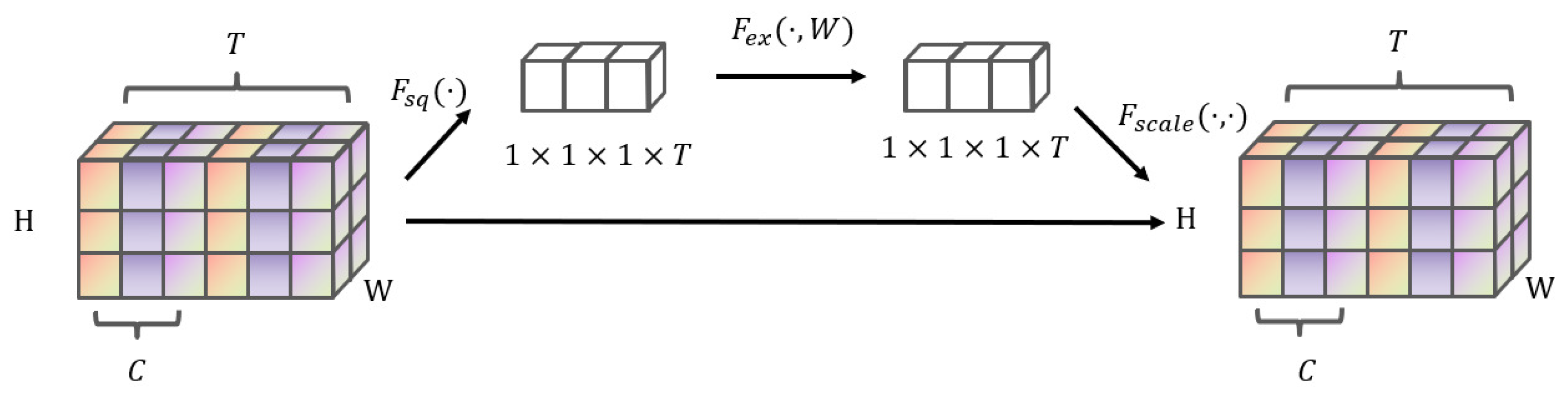
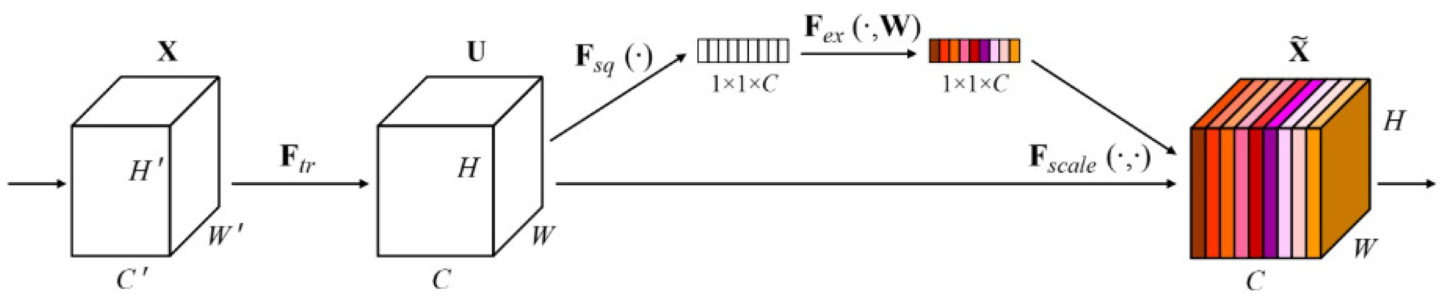
The datacube is a 5D tensor, while the conventional SENet does not account for temporal relationships. Therefore, we have developed a 3D-SENet based on the original SENet [30] to extract temporal information. The model diagram is depicted in Figure 1. The input datacube undergoes a 3D convolution. If the input data is represented as $X\left(\left\{B,T,C,H,W\right\}\right)$, it will be convolved with T kernels of size $\left(C,H,W\right)$. After the $F_{sq}$ operation, a $1\times 1\times 1\times T$ tensor is obtained, followed by the calculation of temporal channel memory. The final output $Y\left(\left\{B,T,C,H,W\right\}\right)$ matches the input dimensions. Here is how we implemented the 3D-SENet. We used one 3D convolutional layer for spatiotemporal feature extraction, with kernel size (1,1,1), stride 1, and padding set to “same” so that the feature dimensions stay the same. The 1 × 1 × 1 3D convolution kernel is a classical and standard configuration for channel–temporal attention calibration modules [30,31,32]. Its core role is to perform channel-wise and temporal-wise feature weight recalibration rather than directly capture large-range spatiotemporal dependencies. The large-range spatiotemporal dependencies of soil moisture have already been fully extracted by the preceding ConvLSTM and GCN modules. Using larger 3D convolution kernels will introduce redundant spatial–temporal sampling, significantly increase the number of model parameters and computational overhead, and easily lead to overfitting, which is not conducive to the stability and lightweight design of the attention mechanism. Therefore, the 1 × 1 × 1 convolution kernel is the optimal choice for the 3D-SENet attention module in this study. After that, we added a global average pooling layer to do the Squeeze operation, followed by two fully connected layers for the Excitation step. The first fully connected layer reduces the feature dimension to one-quarter of the original channel number, and the second restores it back to the original dimension. Both layers use ReLU as the activation function. For the temporal channel memory, we learn weights independently along the time dimension (T) of the 5D input tensor. The spatiotemporal features at each time step are compressed into a 1D feature vector by global average pooling, then the fully connected layers produce an attention weight for each time step. After normalizing these weights with Softmax, we multiply them with the original temporal features and combine everything to obtain the enhanced temporal channel features. This approach affects feature learning in two ways. First, it gives higher weights to the time steps that matter most for soil moisture changes, helping the model learn useful temporal patterns while suppressing noise from less important steps. Second, it captures correlations between channels across the time dimension, so the model can adaptively figure out how much each time step contributes to the prediction. That improves the model’s ability to extract meaningful time-series features.

2.2.5. CTA-GraphConvLSTM

Therefore, we formulated soil moisture prediction as a dense spatial regression task, preserving the spatial grid structure to balance computational cost and prediction accuracy. That means we do not treat moisture as a class label; instead, we borrow the idea of pixel-wise spatial prediction from dense regression models to handle grid-based global predictions. There are three core reasons for choosing this method: first, soil moisture prediction at the global 1° resolution is a continuous value prediction at the grid pixel level, which is highly consistent with the pixel-level output logic of dense spatial regression. Each grid corresponds to a pixel of an image, and the model needs to output a continuous soil moisture value for each pixel, which is essentially pixel-level regression rather than category segmentation; second, compared with direct regression mapping, the modeling method of dense spatial regression can better explore the spatial neighborhood correlation between grids, allowing the model to capture the spatial distribution law of soil moisture and conform to the spatial heterogeneity characteristics of soil moisture; third, this method can greatly reduce the computational cost of global-scale prediction, avoid the massive computation caused by point-by-point regression mapping, and adapt to the spatiotemporal feature extraction architecture of models such as ConvLSTM and GCN to realize the joint learning of temporal and spatial features. Considering the entire globe as a grid with pixel dimensions of $180\times 360$, calculating soil moisture for each grid point presents a substantial computational burden even after excluding ocean areas. Therefore, In this study, the soil moisture prediction task is approached as a dense spatial regression problem, where each grid cell corresponds to a pixel location, but the output is a continuous moisture value rather than a discrete class. In this context, the input variables are represented as $X\left(\left\{B,T,C,H,W\right\}\right)$, and the output of this model is $Y\left(\left\{B,C,H,W\right\}\right)$. This approach substantially reduces the time cost required to predict global soil moisture.

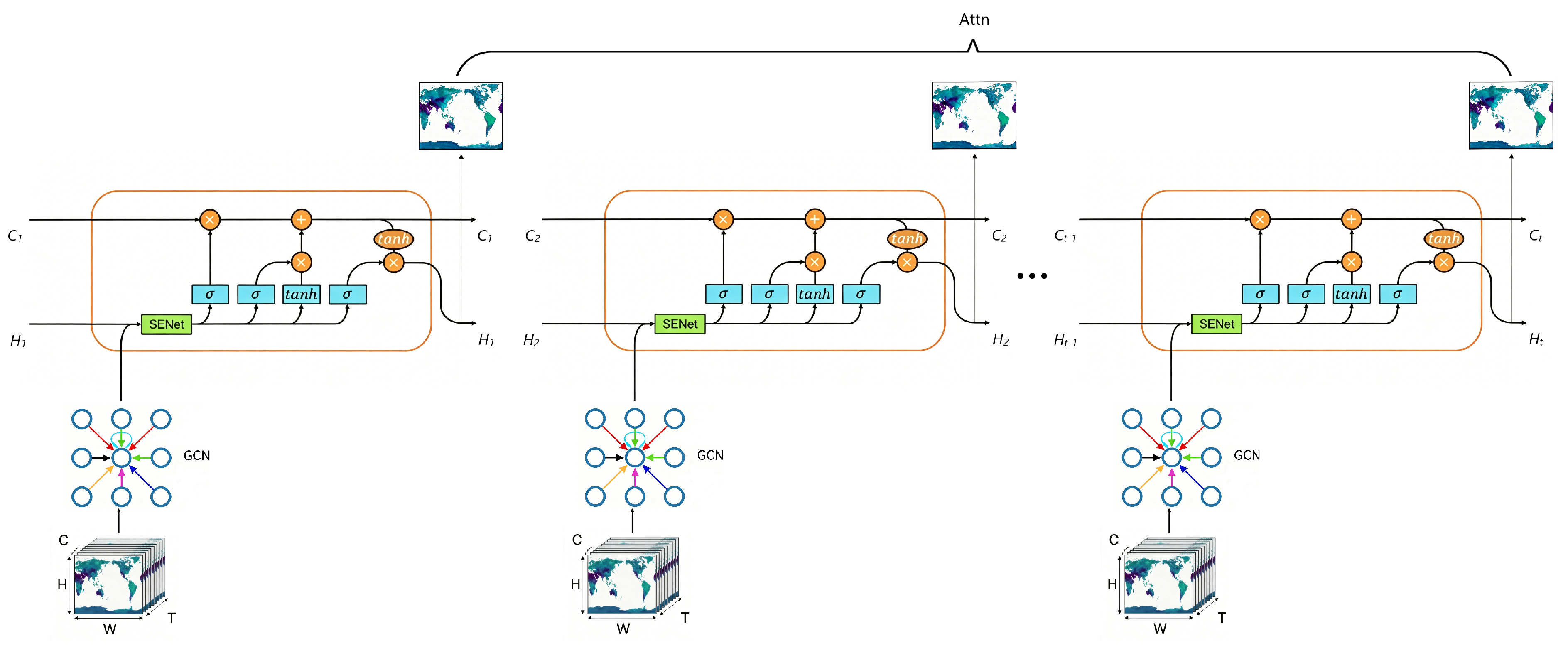
The original ConvLSTM model has been extended by introducing both an attention mechanism and the SENet model, as illustrated in Figure 2. The attention mechanism is employed to extract the temporal information from ConvLSTM, while SENet is used to capture inter-channel correlations. SENet was incorporated before extracting spatial information from ConvLSTM, and the output feature $T_t\in {\mathbb{R}}^{BCHW}$ at each time step was obtained, where B denotes batch size, C is the number of feature channels, and $H,W$ represent the spatial dimensions of the global grid. The attn function defined in this study acts as the core module for calculating feature weights across different time steps, which enables the model to capture temporal and channel attention simultaneously. Derived from the channel attention mechanism of 3D-SENet, the attn function decouples the spatiotemporal features output by each hidden layer of ConvLSTM and assigns adaptive weights to different time channels, with the time channel regarded as the key dimension for attention learning. The channel attention mechanism automatically assigns adaptive weights to all 11 input features. In regions with dense vegetation or strong vegetation–moisture coupling, the model enhances the weight of NDVI to better capture the constraint of vegetation coverage on soil moisture gain and loss. The technical calculation process of attention weights by the attn function is mathematically formulated as follows:

$$GAP\left(T_t\right)\in {\mathbb{R}}^{B\times C},MLP\left(GAP\left(T_t\right)\right)\in {\mathbb{R}}^{B\times C}$$

(2)

$${\alpha }_t=Softmax\left(MLP\left(GAP\left(T_t\right)\right)\right),{\alpha }_t\in {\mathbb{R}}^{B\times C}$$

(3)

$$T_t^{\prime }={\alpha }_t\otimes T_t,T_t^{\prime }\in {\mathbb{R}}^{B\times C\times H\times W}$$

(4)

$$T^{\prime }=\left[T_1^{\prime },T_2^{\prime },\dots ,T_T^{\prime }\right]\in {\mathbb{R}}^{BTCHW}$$

(5)

where $\mathrm{GAP}(·)$ denotes global average pooling, $\mathrm{MLP}(·)$ denotes a multi-layer perceptron with two fully-connected layers and ReLU activation, $\mathrm{Softmax}(·)$ normalizes weights to $[0,1]$. ${\alpha }_t$ is the attention weight at time step t, ⊗ denotes element-wise multiplication, $T_t$ is the output feature of ConvLSTM at time step t, $T_t^{\prime }$ is the attention-weighted feature. $T^{\prime }$ denotes the concatenated overall spatiotemporal feature; B, T, C, H, and W stand for batch size, time step dimension, channel number, spatial height, and spatial width, respectively.

In the formulas above, $T_t$ is the output feature of ConvLSTM at the t-th time step. $GAP(·)$ refers to the global average pooling operation, which compresses the 3D feature map ($CHW$) of each time step into a 1D channel feature vector. This operation not only reduces the dimensionality of spatiotemporal features but also extracts the key information of each feature channel. $MLP(·)$ represents a multi-layer perceptron composed of two fully connected layers with the ReLU activation function in between, which is used to conduct nonlinear transformation of the pooled channel features and learn the potential weight relationship among different time steps. The $Softmax(·)$ function normalizes the transformed feature values to the range of $[0,1]$, generating the attention weight ${\alpha }_t$ for the t-th time step. A larger value of ${\alpha }_t$ indicates a higher contribution of the corresponding time step to the soil moisture prediction task. The symbol ⊗ denotes the element-wise multiplication operation, which weights the original feature $T_t$ with the attention weight ${\alpha }_t$ to obtain the enhanced feature $T_t^{\prime }$. Finally, the enhanced features of all time steps are concatenated to form the output feature $T^{\prime }$ of the attn function, which is the spatiotemporal feature integrated with channel-temporal attention and will be fed into the subsequent GCN layer for spatial feature modeling.

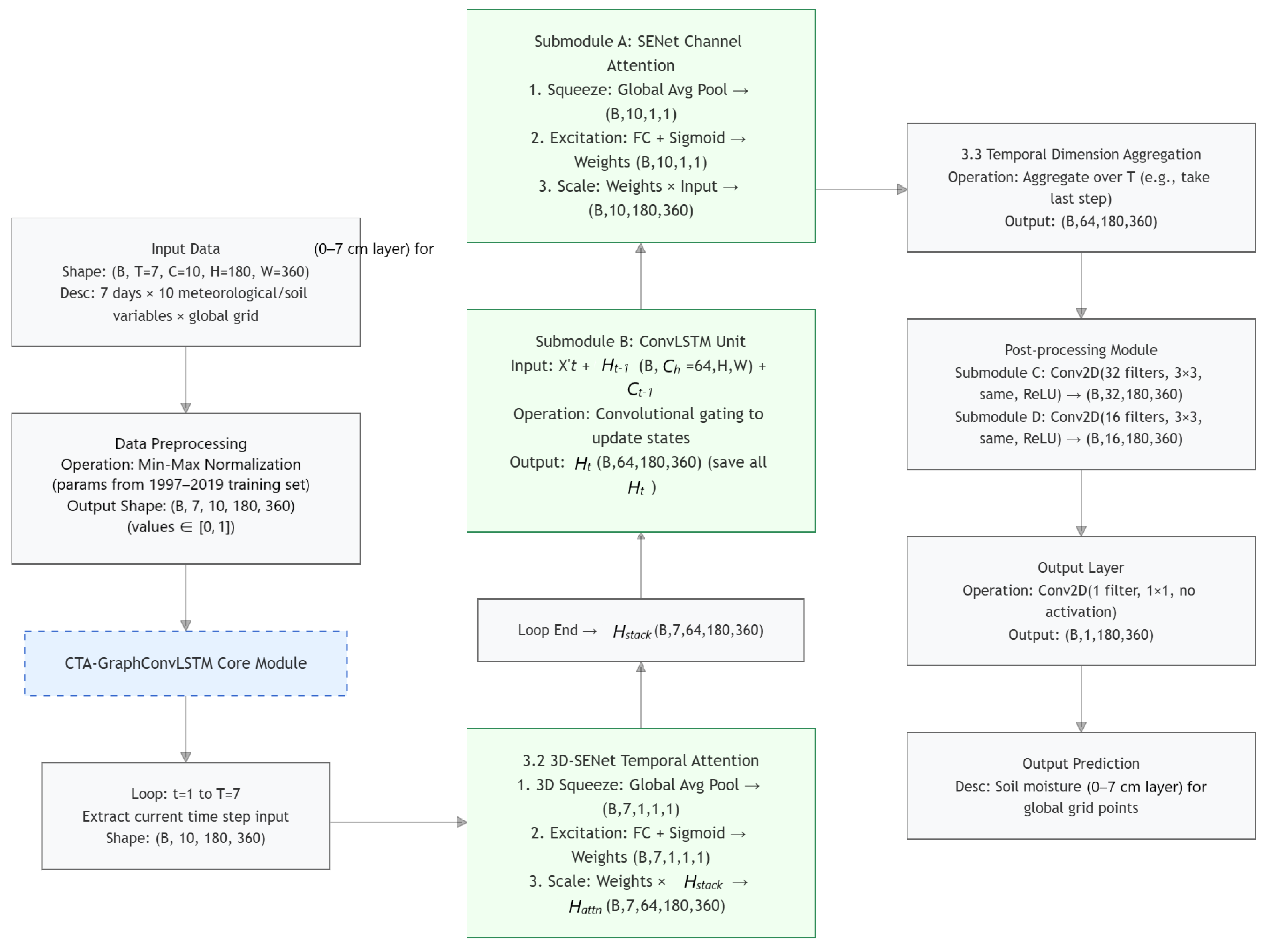
The attn function calculates the 3D-SENet channel attention, where the information from each hidden layer is extracted and the time channel is considered as the one that requires attention. Through the above weighting process, the attn function strengthens the feature learning of key time steps related to soil moisture variations (e.g., periods after precipitation) and suppresses the noise interference from invalid time steps effectively. Assuming the input for each time step is represented as $T\left(\left\{B,T,C,H,W\right\}\right)$, the hidden output remains as $T\left(\left\{B,T,C,H,W\right\}\right)$ after the attention calculation. By applying attention to the time dimension, the calculated weights are multiplied by the ConvLSTM output, enabling the model to focus on the most influential time steps. Traditionally, in image classification tasks, linear layers are added at the end of the model to produce the final output. After ConvLSTM processes spatiotemporal data, two additional convolutional activation layers were introduced with hidden layer sizes of 32 and 16, using $3\times 3$ kernels. This was done to improve the fitting performance of this model. To maintain consistency in output and input image sizes, padding was applied with a value of 1 to the ConvLSTM output. Figure 3 shows the architecture of the CTA-GraphConvLSTM model. It incorporates SENet to capture channel attention in the input data and uses 3D-SENet after each time step to relate them. The key is that the GCN layer is placed at the input stage of the ConvLSTM layer, where the standard convolution operations for spatial feature extraction are replaced or augmented with graph convolutions based on a pre-computed adjacency matrix, enabling the model to learn the irregular spatial dependencies inherent in the global grid. Specifically, we treat the global 180 × 360 grid as a graph $G=(V,E)$, where each grid point is a node V. Different from the fixed 8-neighborhood adjacency, the edge connections in this model are learned adaptively by the graph convolutional layer instead of being limited to geographical proximity. This design enables the model to capture the real soil moisture connectivity dominated by geographical conditions, river systems, groundwater distribution and other hydrological factors, rather than being constrained by simple grid adjacency. In constructing the graph adjacency matrix, we integrated both geographic distance and land use/underlying surface attributes. Nodes with the same or similar underlying surface types are assigned stronger spatial connections, enabling the GCN to capture soil moisture spatial heterogeneity driven by the underlying surface rather than only grid proximity. At each time step of the CTA-GraphConvLSTM, the hidden state $H_t$ is not only updated through the internal gating mechanism of the ConvLSTM but also aggregates information from its neighboring nodes via a graph convolutional layer. This operation can be defined as:

$$H_t^{\prime }=\sigma (A·H_t·W)$$

(6)

where $H_t^{\prime }$ denotes the updated hidden state after graph convolution, $\sigma (·)$ represents the activation function, A is the normalized adjacency matrix, $H_t$ is the original hidden state, and W is a learnable weight matrix. Then, $H_t^{\prime }$, which has aggregated neighborhood information, is fed into the subsequent SENet module.

Treating the soil moisture prediction task as a dense spatial regression task can greatly reduce the time consumed by the model prediction and the spatial information of each neighborhood can also be taken into account. The complete modeling process of CTA-GraphConvLSTM includes four steps: (1) Data input: input standardized meteorological, soil and radiation variables in the form of 5D tensor $\left(\left\{B,T,C,H,W\right\}\right)$; (2) Channel attention: embed SENet before the forget gate of ConvLSTM to adaptively learn channel feature weights; (3) Temporal attention: model global time steps through 3D-SENet to enhance key temporal features; (4) Output optimization: add two convolutional activation layers with hidden dimensions of 32 and 16 in turn, 3 × 3 kernels and padding = 1, and finally output soil moisture prediction results in $\left(\left\{B,C,H,W\right\}\right)$ format. Key hyperparameters of the model: time window T = 7, batch size = 64, maximum iterations = 500, dropout = 0.15, and ReLU activation function. The model adopts a fused architecture of graph convolution and spatiotemporal attention, which does not need to directly process raw remote sensing images. It only needs to input standardized surface variables and is naturally compatible with the input formats of various types and resolutions of remote sensing data. The model only needs to perform unified min-max normalization on the input data to adapt to different remote sensing data sources without adjusting the core network structure.

Figure 4 provides a holistic view of the data flow and the interplay among the different modules. As depicted, the input 5D tensor $X\in {\mathbb{R}}^{B\times T\times C\times H\times W}$ first undergoes min-max normalization. For each time step t, the current slice $X_t$ is recalibrated by the SENet channel attention module, which adaptively weights the feature channels. The recalibrated feature map is then passed into a ConvLSTM cell that updates the hidden state $H_t$ and cell state $C_t$ by incorporating spatial context via convolutional gates. After processing all T time steps, the stacked hidden states $H\in {\mathbb{R}}^{B\times T\times C_h\times H\times W}$ are fed into the 3D-SENet temporal attention module. This module computes importance weights along the time dimension and re-weights the hidden states accordingly, enabling the model to focus on the most informative time steps. The temporally attended features are then aggregated (e.g., by taking the last time step) and refined by two subsequent convolutional layers with 32 and 16 filters, respectively. Finally, a $1\times 1$ convolution maps the features to a single channel, producing the predicted soil moisture map $\widehat{Y}\in {\mathbb{R}}^{B\times 1\times H\times W}$ for the 0–7 cm layer. This end-to-end architecture effectively captures both channel-wise and temporal dependencies while preserving spatial structures, which is key to its improved performance.

2.3. Model Performance Assessment

All comparison models in this study adopt completely unified experimental settings, and only the network structure is different to ensure fair comparison. The unified settings include: training set (1997–2019), test set (2020), time window 7, batch size 64, dropout = 0.15, and min-max normalization. 1-day and 5-day ahead predictions are selected as typical time scales for performance evaluation. The soil moisture values for lead times of 1 day and 5 days were selected as the target variables. The dataset was divided into training and testing sets. The data from 1 January 1997 to 31 December 2019 was used as the training dataset. During training, the generation with the lowest loss was recorded as the final testing model. To comprehensively and multi-dimensionally evaluate the regression performance of the soil moisture prediction model, we selected bias (Bias), root mean square error (RMSE), correlation coefficient (R), coefficient of determination $R^2$, Kling-Gupta Efficiency (KGE) and unbiased root mean square error (ubRMSE) as the core evaluation metrics, and did not adopt the mean absolute error (MAE). The core selection basis and the impact of metric selection on result interpretation are as follows: the selected metrics cover three key dimensions of regression model performance evaluation. Systematic deviation (Bias) measures the average deviation between predicted and true values, reflecting whether the model has systematic overestimation or underestimation. Overall error (RMSE/ubRMSE) quantifies the root mean square error with and without systematic deviation, respectively, to evaluate the overall prediction accuracy of the model. Linear correlation ($R/R^2$) characterizes the linear correlation and goodness of fit between predicted and true values, reflecting the model’s ability to capture the spatiotemporal variation law of soil moisture. KGE is a classic comprehensive metric in hydrological simulation that integrates correlation, variability and mean bias to compensate for the limitations of single metrics. The synergy of the five metrics enables a comprehensive evaluation of model performance and avoids the one-sidedness of interpretation with a single metric. The optimal model is selected by the lowest validation RMSE and highest validation $R^2$, and all metrics are used for comprehensive result interpretation. MAE was not selected because it weights all prediction errors equally and has low sensitivity to extreme errors. However, this study focuses on global-scale soil moisture and drought level prediction, where extreme soil moisture anomalies (e.g., severe drought, extreme wetness) are the core concerns of drought early warning and precision agriculture. RMSE’s high sensitivity to extreme errors is more in line with the practical application needs of this study, and can effectively reflect the model’s prediction ability for extreme hydrological scenarios. Metric selection directly determines the focus of result interpretation: focusing only on correlation while ignoring error metrics may overlook the actual prediction accuracy of the model; focusing only on error while ignoring correlation cannot judge whether the model captures the inherent variation law of soil moisture. Joint evaluation with multiple metrics enables an objective and comprehensive interpretation of model performance, and provides targeted directions for model optimization. Finally, bias, root mean square error (RMSE), correlation coefficient (R) and KGE were chosen as performance evaluation metrics [33,35]. Bias measures systematic deviations from actual values, R quantifies the degree to which the model captures data variations, and RMSE assesses the accuracy of the model in predicting volatility. These metrics serve as reliable indicators for the overall performance evaluation of both data-driven deep learning models and process-based models. Furthermore, R-squared ($R^2$) and unbiased root mean square error ($ubRMSE$) are utilized to assess the performance of the model.

They are defined as follows:

$$RMSE=\sqrt{{\displaystyle \frac{{\sum }_{k=1}^N{\left(x_i-y_i\right)}^2}{N}}}$$

(7)

$$R={\displaystyle \frac{{\sum }_{i=1}^N\left(x_i-\overline{X}\right)\left(y_i-\overline{Y}\right)}{\sqrt{\left({\sum }_{i=1}^n{\left(x_i-\overline{X}\right)}^2\right)}\sqrt{{\sum }_{i=1}^n{\left(y_i-\overline{Y}\right)}^2}}}$$

(8)

$$Bias={\displaystyle \frac{{\sum }_{i=1}^N\left(x_i-y_i\right)}{N}}$$

(9)

$$R^2=1-{\displaystyle \frac{{\sum }_{i=1}^n{\left(y_i-x_i\right)}^2}{{\sum }_{i=1}^n{\left(y_i-\overline{Y}\right)}^2}}$$

(10)

$$ubRMSE=\sqrt{{\displaystyle \frac{{\sum }_{k=1}^N{\left(\left(x_i-\overline{X}\right)-\left(y_i-\overline{Y}\right)\right)}^2}{N}}}$$

(11)

$$KGE=1-\sqrt{{(r-1)}^2+{(\alpha -1)}^2+{(\beta -1)}^2}$$

(12)

where $y_i$ and $x_i$ represent the ground truth and prediction for the i-th time step, respectively. $\overline{Y}$ and $\overline{X}$ are the respective mean values for ground truth and predictions. N represents the total number of samples. ${\sigma }_x$ and ${\sigma }_y$ represent the standard deviations of the predicted and observed values, respectively. r is the Pearson correlation coefficient; $\alpha ={\sigma }_x/{\sigma }_y$ denotes the ratio of standard deviations between predictions and observations; $\beta =\overline{X}/\overline{Y}$ denotes the ratio of mean values between predictions and observations. The range of KGE is $(-\infty ,1]$, and a value closer to 1 indicates better model performance.

The Soil Water Deficit Index (SWDI) performs well in defining the level and severity of drought [36]. The calculation of SWDI is as follows:

$$SWDI=\left({\displaystyle \frac{\theta -{\theta }_{FC}}{{\theta }_{AWC}}}\right)\times 10$$

(13)

$${\theta }_{AWC}={\theta }_{FC}-{\theta }_{WP}$$

(14)

where $SWDI$ denotes the Soil Water Deficit Index, $\theta$ represents the time series of ERA5-Land soil moisture or model-predicted soil moisture, and ${\theta }_{FC}$, ${\theta }_{WP}$ and ${\theta }_{AWC}$ denote field capacity, wilting point, and available water capacity, respectively. There are various methods to define ${\theta }_{FC}$ and ${\theta }_{WP}$. In this study, we chose the 18th and 346th soil moisture values from the time series to represent ${\theta }_{FC}$ and ${\theta }_{WP}$. This selection is grounded in solid scientific rationale, aligning with both the statistical properties of the ERA5-Land dataset and established norms in agricultural hydrology. For the ERA5-Land 0–7 cm soil moisture time series (sorted in ascending order), the 18th quantile corresponds to the critical state where soil retains maximum capillary water after saturated drainage—directly matching the hydrological definition of ${\theta }_{FC}$ (field capacity), the upper limit of plant-available water. The 346th quantile reflects the minimum soil moisture at which plants undergo permanent wilting, consistent with the core characteristic of ${\theta }_{WP}$ (wilting point), the lower limit of plant-available water. This quantile-based approach is consistent with the Specifications for Agricultural Meteorological Observation and widely adopted in mainstream studies on soil moisture retrieval and drought index calculation [36,37]. It ensures the rationality of ${\theta }_{FC}$ and ${\theta }_{WP}$ characterization, laying a reliable foundation for accurate SWDI-based drought level classification. The daily SWDI is calculated based on the time series of soil moisture from each grid point in the ERA5-Land dataset and the predicted soil moisture data from the model. All data processing, statistical analysis and programming modeling in this study were implemented using Python 3.10.

3. Experiments and Results

3.1. Performance Evaluation of Models

We compared our model against three baselines—LSTM, GraphLSTM, and ConvLSTM—using 1-day and 5-day ahead predictions.

Table 5. Performance evaluation of different models for 1-day lead time soil moisture prediction.

Model	R	${\mathit{R}}^2$	$\mathit{RMSE}$	$\mathit{ubRMSE}$	$\mathit{Bias}$	$\mathit{KGE}$
LSTM	0.768	0.430	0.038	0.032	0.029	0.581
GraphLSTM	0.661	0.088	0.048	0.041	0.037	0.223
ConvLSTM	0.783	0.444	0.037	0.031	0.027	0.602
CTA-GraphConvLSTM	0.815	0.555	0.032	0.029	0.023	0.710

lists results for 1-day prediction, and

Table 6. Performance evaluation of different models for 5-day lead time soil moisture prediction.

Model	R	${\mathit{R}}^2$	$\mathit{RMSE}$	$\mathit{ubRMSE}$	$\mathit{Bias}$	$\mathit{KGE}$
LSTM	0.611	0.162	0.044	0.040	0.036	0.384
GraphLSTM	0.492	−0.121	0.053	0.047	0.042	0.103
ConvLSTM	0.643	0.230	0.042	0.039	0.032	0.422
CTA-GraphConvLSTM	0.666	0.313	0.039	0.038	0.030	0.623

for 5-day prediction. Our CTA-GraphConvLSTM performs best across every metric. GraphLSTM comes out weakest, mostly because LSTM is designed for time-series data and GraphLSTM does not handle spatial structure well. However, when dealing with fused temporal and spatial data, it cannot accurately output data structured in space as effectively as the CTA-GraphConvLSTM.

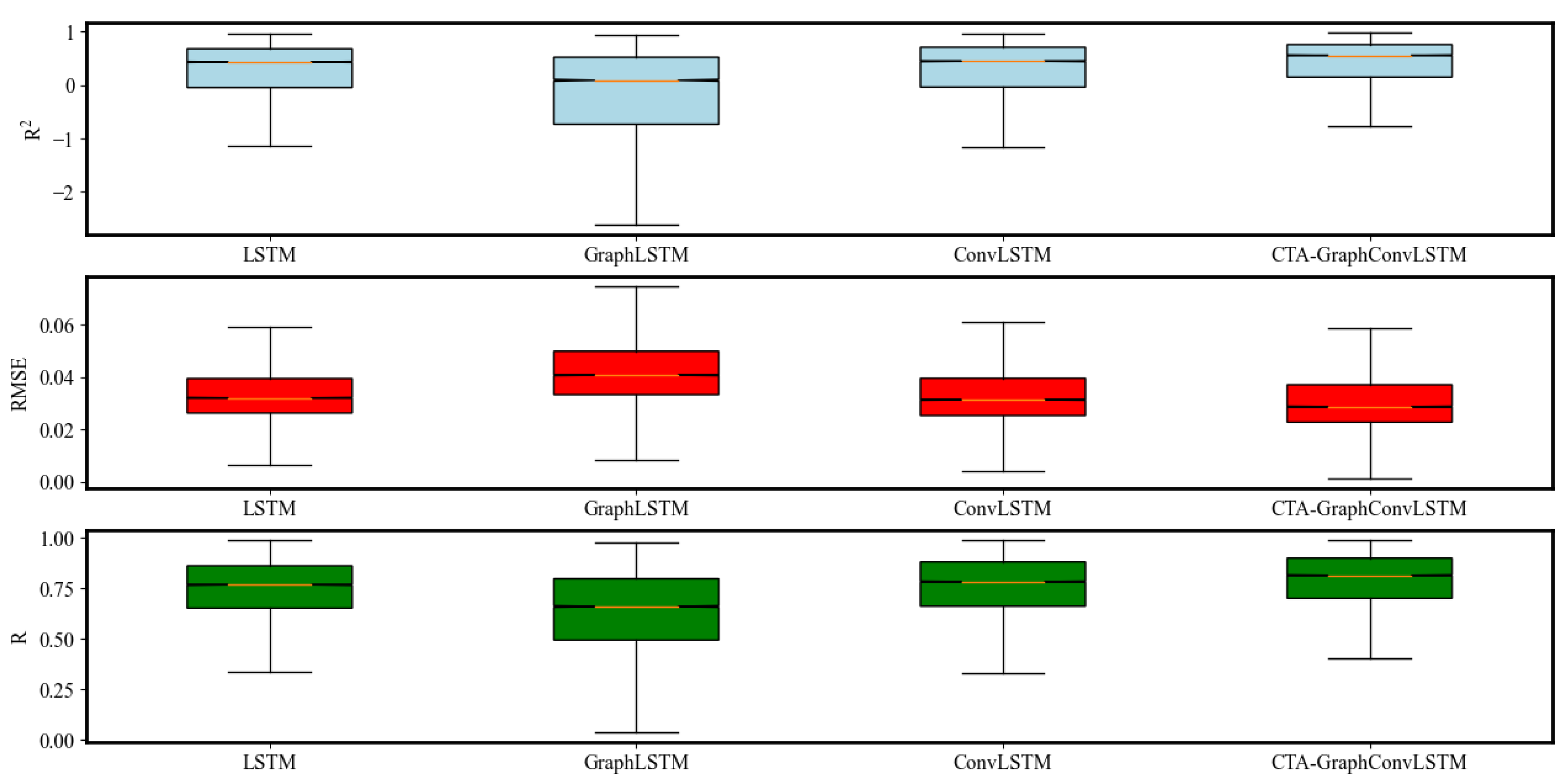
The soil moisture prediction task was treated as a regression task for dense spatial regression, employing random sampling during data collection, setting a temporal window of 7 time steps, and predicting soil moisture values for 1 day and 5 days ahead. In the data collection phase, a spatiotemporal stratified random sampling strategy was adopted to ensure the spatial and temporal randomness of the dataset. In the spatial dimension, the global 1° resolution soil moisture grids were divided into 5 spatial layers according to climatic zones: tropical, subtropical, temperate, frigid and alpine zones. Random samples were drawn within each layer to ensure that the samples covered regions with different topographies, climates and land use types worldwide, thus avoiding the spatial concentration bias of samples. In the temporal dimension, the daily data from 1997 to 2020 were divided into temporal layers by year and season, and random sampling was conducted proportionally within each temporal layer. This ensured the uniform distribution of samples in different years, four seasons and drought/flood periods, while the sample proportion of each temporal layer was consistent with that of the original data. In addition, grid data with no practical significance for soil moisture observation (e.g., oceans and glaciers) were excluded during sampling. Finally, the spatial distribution of the sampled dataset was guaranteed to cover the main land areas of the world, and the temporal distribution covered the climatic characteristics of different time scales, which effectively avoided the sample selection bias in both spatial and temporal dimensions. After constructing the dataset, deep learning models were used for training, and upon completion, the test data from the year 2020 was evaluated. Finally, we used box plots to display the R-squared ($R^2$), $RMSE$, and R for the four models. Figure 5 depicts the box plots for the models, including the baseline LSTM, GraphLSTM, ConvLSTM, and the proposed CTA-GraphConvLSTM in this experiment, specifically for the prediction of 1 day ahead. It is evident that the GraphLSTM model performed the worst, with both the median and mean values being the lowest among the four models, followed by LSTM, while the experimental results for ConvLSTM were superior to LSTM. The proposed CTA-GraphConvLSTM exhibited the best performance among the four models, with its $R^2$ of 0.555, R of 0.815, and $RMSE$ of 0.032. Therefore, treating soil moisture prediction as a dense spatial regression is a viable approach.

ConvLSTM was introduced to ensure that the model simultaneously focuses on both temporal and spatial data features, which combines the characteristics of both LSTM and CNN, enabling the learning of temporal and spatial features, and the proposed CTA-GraphConvLSTM exhibited the best performance among the four models. Therefore, treating soil moisture prediction as a dense spatial regression is a viable approach.

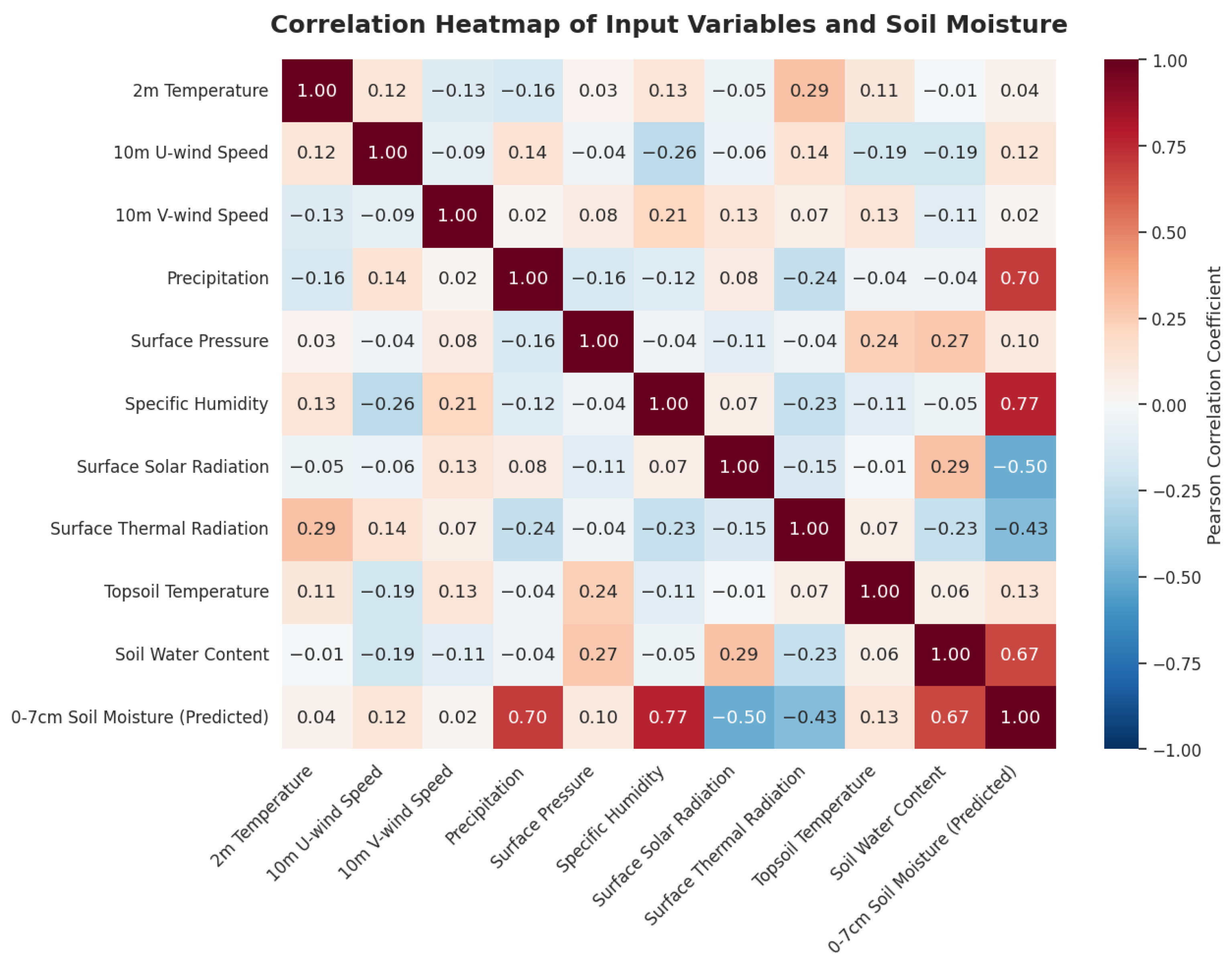
To further explain the rationality of input features and the model performance in different regions, the correlation heatmap of input variables and the sector heatmap of model performance are plotted (Figure 6 and Figure 7).

Figure 6 shows the Pearson correlation between input variables and 0–7 cm soil moisture. Precipitation, specific humidity, NDVI and soil water content exhibit strong positive correlations with soil moisture, while solar radiation shows a negative correlation. The significant positive correlation between NDVI and soil moisture verifies that vegetation coverage is a key driving factor of soil moisture changes, confirming the rationality of introducing NDVI as a characterization feature of vegetation coverage. From a physical perspective, the strong positive correlations of precipitation, specific humidity, and soil water capacity (consistent with soil water content) align with the mechanism that precipitation replenishes soil water and atmospheric humidity directly affects surface water exchange, while the negative correlation of surface solar radiation agrees with the fact that strong radiation accelerates evapotranspiration and reduces soil moisture. Moreover, the absolute correlation coefficients between most input variables remain below 0.3, indicating no severe multicollinearity, which ensures stable model training and reliable feature extraction and prevents redundant information from interfering with feature extraction. The correlation intensity of each variable is consistent with the physical driving factors of soil moisture, demonstrating that the ten input variables selected in this study effectively represent the main meteorological, soil, and radiation conditions affecting spatiotemporal changes in soil moisture. Consequently, this correlation heatmap provides strong and direct support for the reliability of the entire model setup: the consistent positive/negative correlation patterns confirm that the selected variables follow real hydrological and energy exchange processes, ensuring that the model learns physically meaningful spatiotemporal features rather than spurious relationships. Together, these results statistically validate that the input feature system is reasonable, robust, and well-suited for global soil moisture prediction, while also offering a statistical foundation for explaining the model’s prediction performance across different climatic regions.

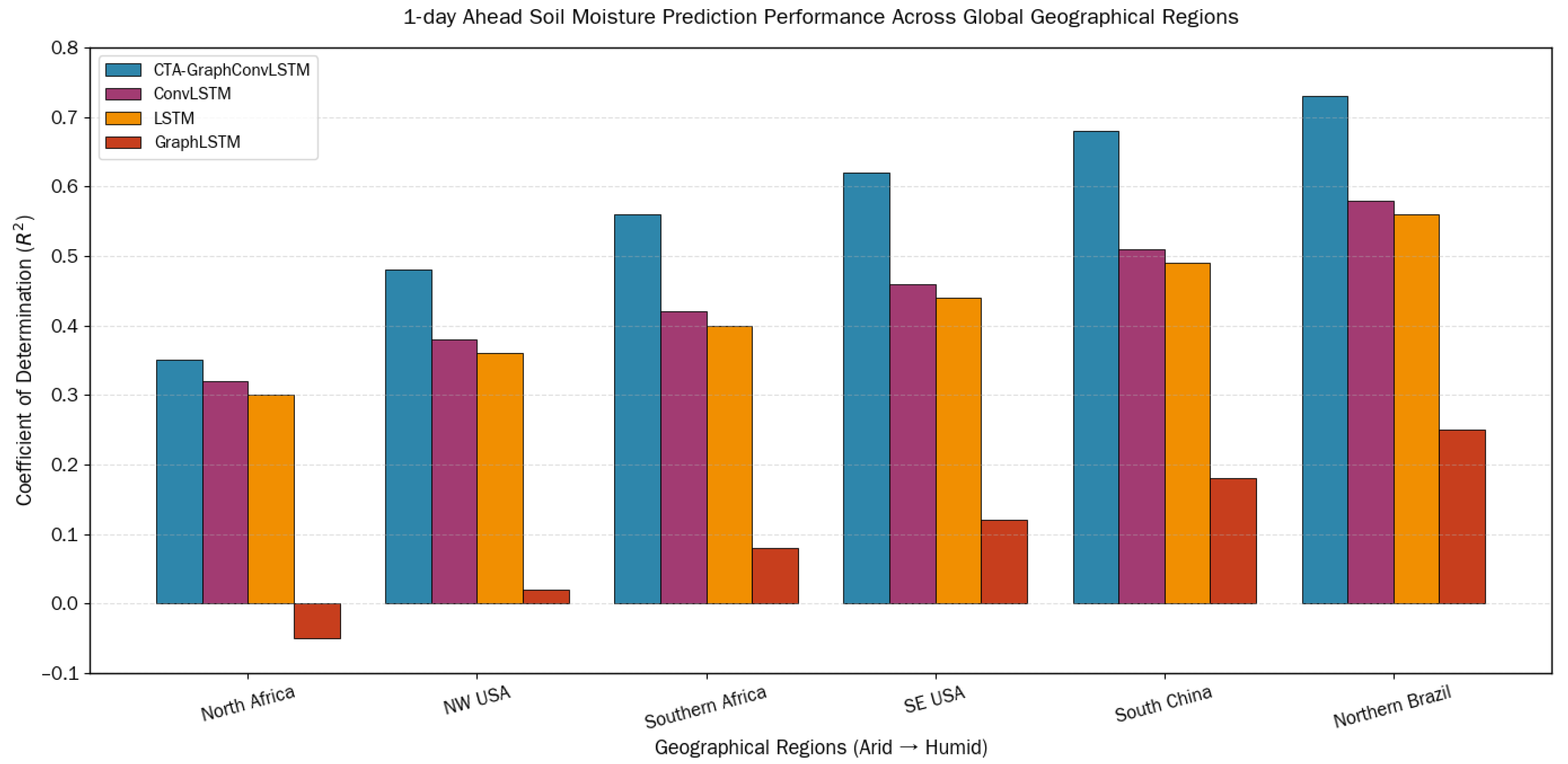
Figure 7 presents the $R^2$ sector heatmap of four models in six typical regions. The CTA-GraphConvLSTM achieves the best performance in all regions, and the performance in humid regions (Southern China, Northern Brazil) is significantly higher than that in arid regions (North Africa). GraphLSTM outperforms LSTM, and ConvLSTM is slightly better than GraphLSTM, indicating that spatial features and graph structure can effectively improve the prediction accuracy of soil moisture.

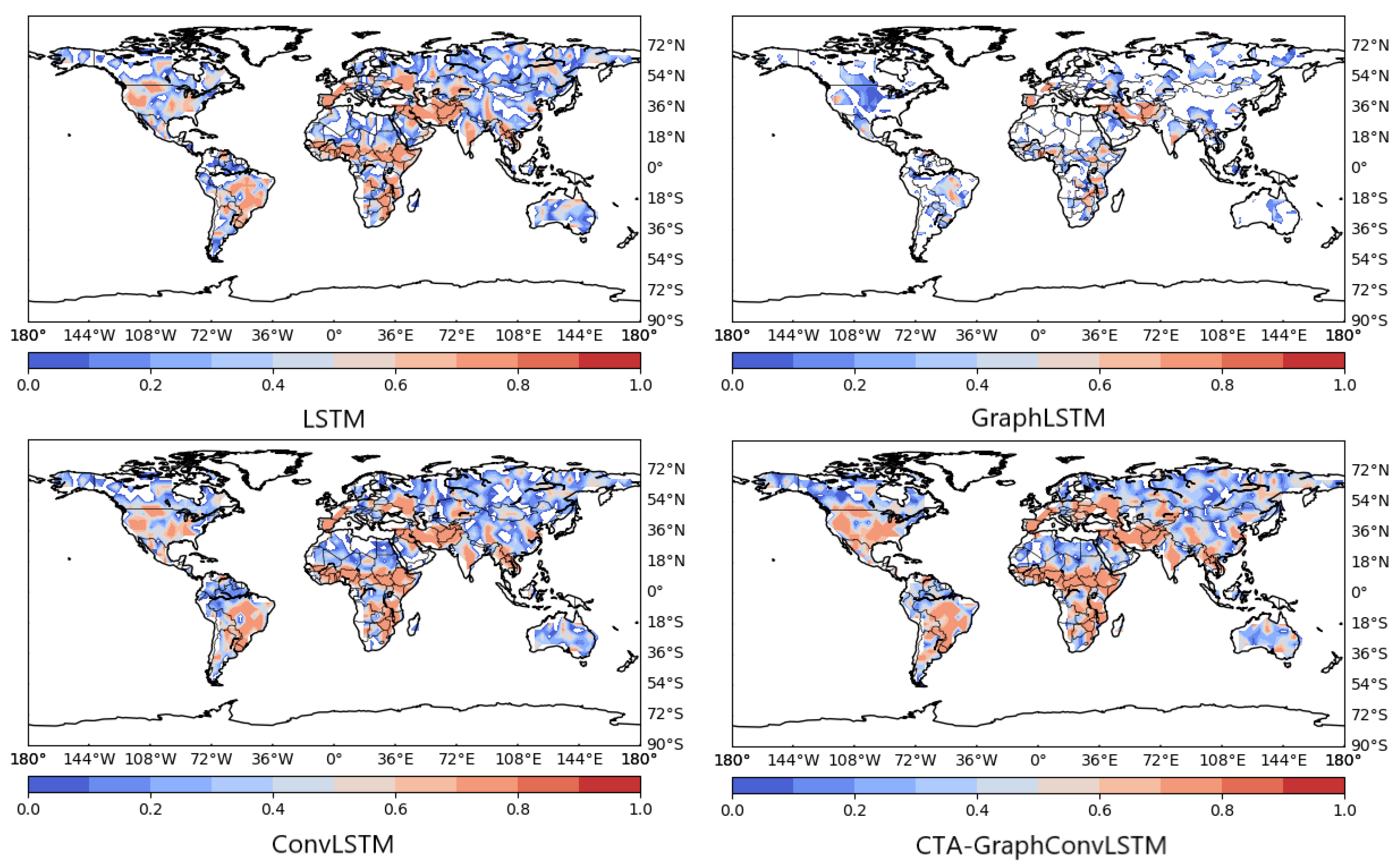
Figure 8 presents the per-grid $R^2$ spatial distribution for the four models at a 1-day lead. Overall, LSTM, ConvLSTM, and CTA-GraphConvLSTM achieve $R^2$≥ 0 in most global land areas, though with varying magnitudes across regions. The CTA-GraphConvLSTM model maintains stable and high accuracy across different land use and underlying surface types. It performs particularly well over cultivated land, forest, and grassland with regular moisture dynamics, and still achieves reliable prediction in ecotones and heterogeneous underlying surfaces by using land use–constrained graph convolution. In stark contrast, GraphLSTM exhibits negative $R^2$ (white areas in Figure 8) not as sporadic isolated points but as continuous patches highly concentrated in typical arid and semi-arid regions, including the Sahara Desert in North Africa, the Arabian Peninsula, Central Asia, and central Australia. This spatial pattern strongly suggests that the failure of GraphLSTM is closely linked to the unique hydrological and surface characteristics of arid zones.

The key features of soil moisture in arid regions include persistently low values (usually below 0.1 m³/m³), small temporal variability, and poor spatial continuity—soil moisture between adjacent grids often lacks stable spatial correlation due to sandy soil textures, sparse vegetation, and intermittent precipitation. GraphLSTM struggles precisely under such conditions. The model suffers from two fundamental structural limitations. First, it forcibly incorporates a graph structure into the original LSTM framework while completely removing convolutional operations. This means that, unlike ConvLSTM, GraphLSTM cannot extract local spatial features through convolutional kernels; it can only propagate information via a pre-defined adjacency matrix. In arid regions where the spatial autocorrelation of soil moisture is already weak, this graph modeling approach—lacking local feature extraction—easily amplifies noise into erroneous spatial signals. Second, the adjacency matrix of GraphLSTM is constructed based on a simple spatial neighborhood (e.g., eight-neighbor connectivity) on a regular 1° grid, which severely mismatches the actual hydrological connectivity in arid zones. In deserts such as the Sahara, the factors that truly influence soil moisture distribution are often dune field orientations, groundwater depth, or occasional ephemeral river networks—not regular rectangular neighborhoods. Consequently, the graph structure of GraphLSTM not only fails to provide effective spatial priors but also introduces spurious spatial constraints unrelated to physical processes.

The combined effect of these two deficiencies is that, in arid regions, the prediction error of GraphLSTM even exceeds the natural variability of soil moisture itself, driving $R^2$ into negative values (white areas). In other words, GraphLSTM predicts worse than simply using the historical mean in these arid zones. By contrast, ConvLSTM preserves local spatial smoothness through standard convolution, and CTA-GraphConvLSTM further adaptively captures irregular spatial dependencies via learnable graph convolutions. Hence, neither model exhibits systematic white areas in the same arid regions. This spatial diagnosis unequivocally confirms that the extremely poor performance of GraphLSTM is not accidental but a necessary consequence of its structural inability to project spatial patterns in arid areas.

To further verify the advancement of the proposed model, we supplemented a comparative analysis with three recent deep learning models specially designed for soil moisture prediction. The physically guided LSTM model [38] is constructed for the global scale by embedding hydrological physical priors into the LSTM network, but it does not introduce graph convolution and attention mechanism, so it cannot capture the non-Euclidean spatial correlation and key temporal features of soil moisture. The graph convolution ConvLSTM fusion model [39] is designed for regional scales. Although it combines a graph neural network to improve the ability of spatial feature extraction, it only adopts single temporal attention without constructing a channel-temporal dual attention mechanism, which is difficult to adapt to global 1° resolution heterogeneous grid data. The hybrid physically guided deep learning model [40] is used for global soil moisture simulation, which only relies on traditional convolution modeling and lacks adaptive graph convolution and dual attention mechanism, resulting in poor modeling effect on irregular hydrological connectivity in arid regions. In contrast, the CTA-GraphConvLSTM model proposed in this study realizes the deep integration of graph convolution spatial modeling, ConvLSTM spatiotemporal feature extraction, SENet channel attention and 3D-SENet temporal attention, and innovatively transforms global soil moisture prediction into an image segmentation regression task. While ensuring lightweight, it can not only adapt to the spatial heterogeneity of global 1° resolution grids, but also accurately capture the non-Euclidean hydrological characteristics in arid regions, showing significant advantages in model structure rationality and global scale adaptability.

3.2. Model Predictions and Performance Spatial Distribution

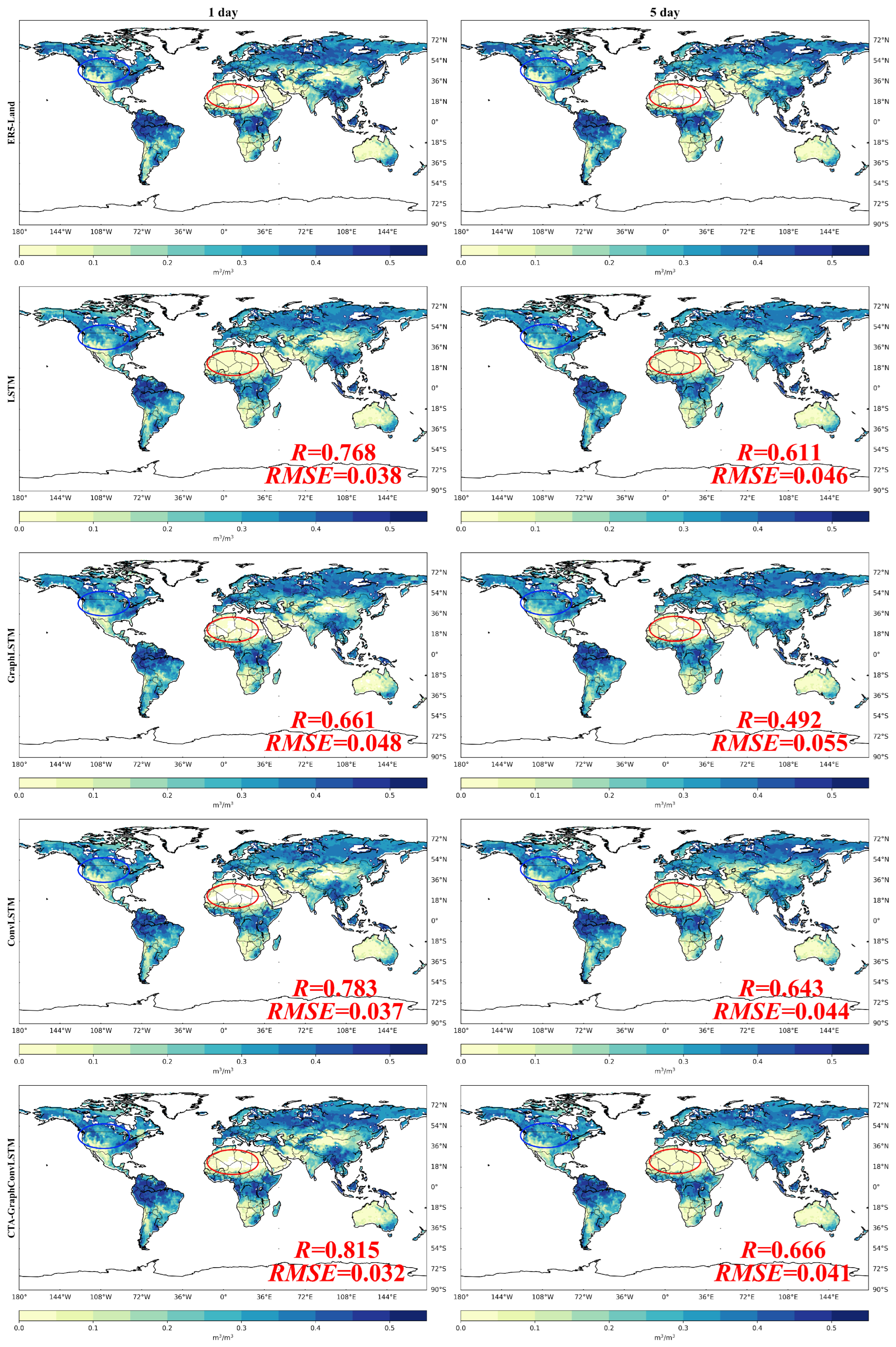
Based on global 1° resolution data, the measured and predicted values of each model are visualized to compare the spatial prediction accuracy in typical regions such as arid and humid areas. The observed and predicted soil moisture values for one day and five days in advance for the four models are shown in Figure 9. The left side of the top row shows the observations for one day in advance, while the right side displays the observations for five days in advance. Subsequently, the predictions are shown for each of the four models: LSTM, GraphLSTM, ConvLSTM and CTA-GraphConvLSTM. Figure 9 compares the observed and predicted soil moisture at 1-day and 5-day lead times. All four models can correctly identify high soil moisture areas, including southern China, northern Brazil, southeastern United States, and south-central Africa. In the northwestern United States marked by the blue ellipse in Figure 9, CTA-GraphConvLSTM matches the ERA5-Land ground truth best. Its graph convolution structure captures spatial connections among neighboring grids, and the temporal attention enhances key meteorological features. In contrast, LSTM lacks spatial modeling, and ConvLSTM only extracts local spatial features, leading to larger errors in this region. In the extremely arid area of northern Africa (red ellipse in Figure 9), CTA-GraphConvLSTM accurately reproduces the severe water scarcity. ConvLSTM overestimates dryness because its local convolution cannot adapt to large-scale homogeneous arid zones, and the absence of 3D-SENet temporal attention weakens its ability to learn long-term drought patterns. When the lead time extends to 5 days (red and blue ellipses on the right of Figure 9), prediction errors rise for all models due to accumulated spatiotemporal noise. However, CTA-GraphConvLSTM shows the mildest performance drop, as the channel-temporal attention filters out redundant information and stabilizes long-term predictions. This phenomenon is reflected in all different DL models, as highlighted by the red and blue ellipses on the right side of Figure 9, pointing out notable regions.

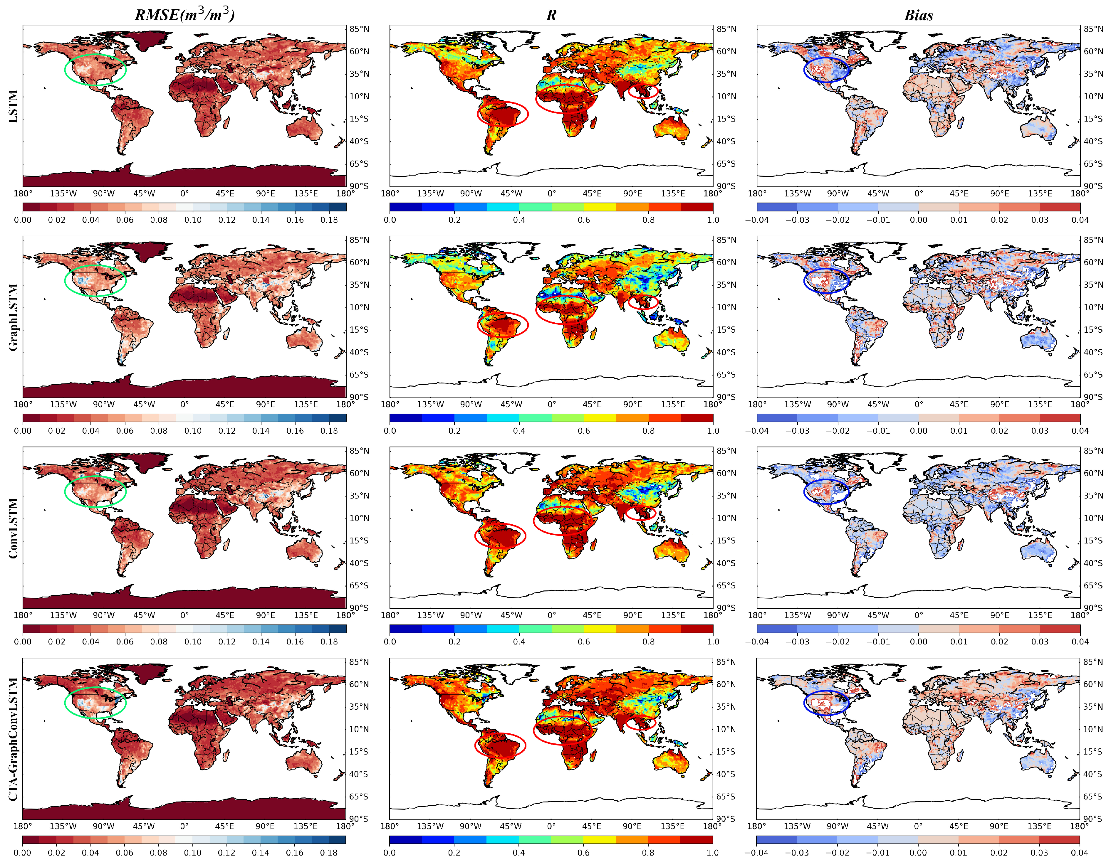
After presenting the predictions of different models, we also used median $RMSE$, R, and $Bias$ at a 1-degree spatial resolution to validate the performance of various deep learning prediction models. Figure 10 demonstrates the predictive performance of different models, specifically for predicting soil volumetric water content at 0–7cm depth. In Figure 10, Figure 10 evaluates the 1-day-ahead prediction performance using RMSE, correlation coefficient R, and Bias. In the northwestern United States (blue ellipse), ConvLSTM (graph-to-point) has slightly lower RMSE than CTA-GraphConvLSTM (graph-to-graph). This is because graph-to-point prediction focuses on single-grid fitting, which suits strong local heterogeneity here, while graph-to-graph prediction performs better in regional overall fitting. In the area marked by the green ellipse, GraphLSTM performs much worse than other models with low R and high RMSE. The tensor reshaping in GraphLSTM breaks the spatiotemporal coupling of soil moisture, making it unsuitable for global-scale data. High R values appear in southern China, northern Brazil, and south-central Africa (red ellipse) for all models. These regions have dense vegetation and stable soil moisture dynamics, so models can easily capture their spatiotemporal patterns. Irregular Bias patterns in the blue ellipse are found in GraphLSTM and CTA-GraphConvLSTM. As typical features of graph-to-graph prediction, neighboring grid information fusion causes slight discontinuities in areas with sharp surface heterogeneity, which provides a clear direction for further model improvement.

3.3. Evaluation Across Various Time Scales

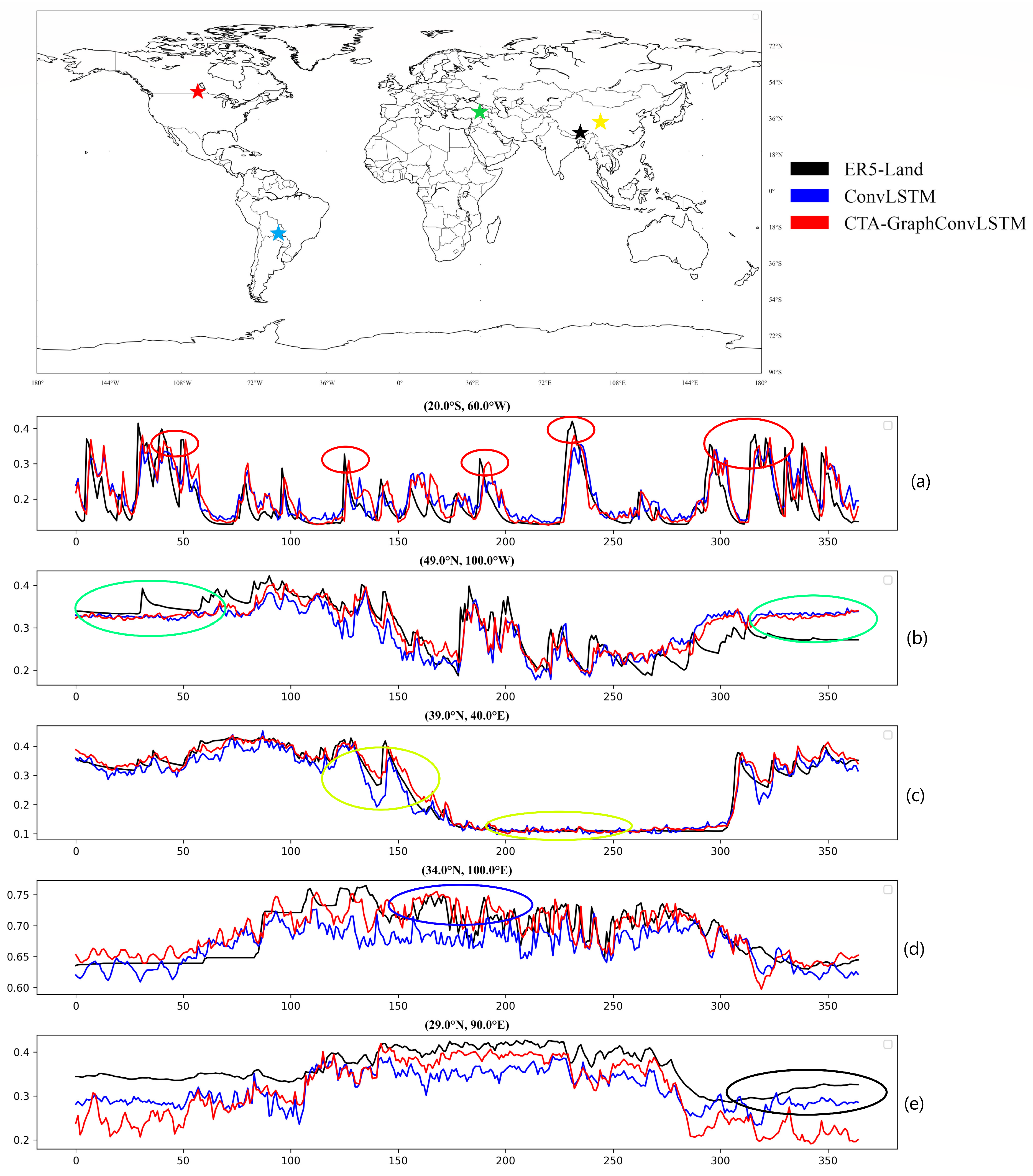
To verify the temporal fitting ability of the models, ConvLSTM and CTA- GraphConvLSTM with the best performance are selected, and 5 global grid points are randomly selected for temporal variation comparison. To assess the temporal variations in predictions, we used the two best models, ConvLSTM and CTA-GraphConvLSTM, both with a time step of 7, predicting soil moisture 1 day ahead. The main difference between them is the nature of the segmentation task. We randomly selected 5 grid points and compared their predictions of soil moisture one year later with the actual values. Figure 11 compares the 1-day-ahead soil moisture time series of ConvLSTM and CTA-GraphConvLSTM at five random grid points. In the peak interval marked by the red ellipse, CTA-GraphConvLSTM accurately captures the peak value and timing, while ConvLSTM underestimates the peaks. The 3D-SENet temporal attention in CTA-GraphConvLSTM strengthens critical time steps of extreme values, but ConvLSTM lacks this mechanism and loses peak features. In the small-fluctuation zone (green ellipse), neither model fully fits the observations. Small fluctuations are high-frequency noise beyond the feature extraction range of spatiotemporal models, which is a common limitation. In the stable change area (yellow ellipse), both models correctly track the trend, showing the strength of spatiotemporal models in modeling steady signals. In the sharp fluctuation region (blue ellipse), CTA-GraphConvLSTM has much higher accuracy. Its channel attention selects key input variables driving fluctuations, improving the capture of sudden changes. In the local area marked by the black ellipse, ConvLSTM performs better. This grid has extremely strong neighboring heterogeneity, and the single-grid fitting of graph-to-point prediction is more targeted. This proves that graph-to-point and graph-to-graph predictions have different applicable scenarios.

3.4. Performance in Drought Level Forecast

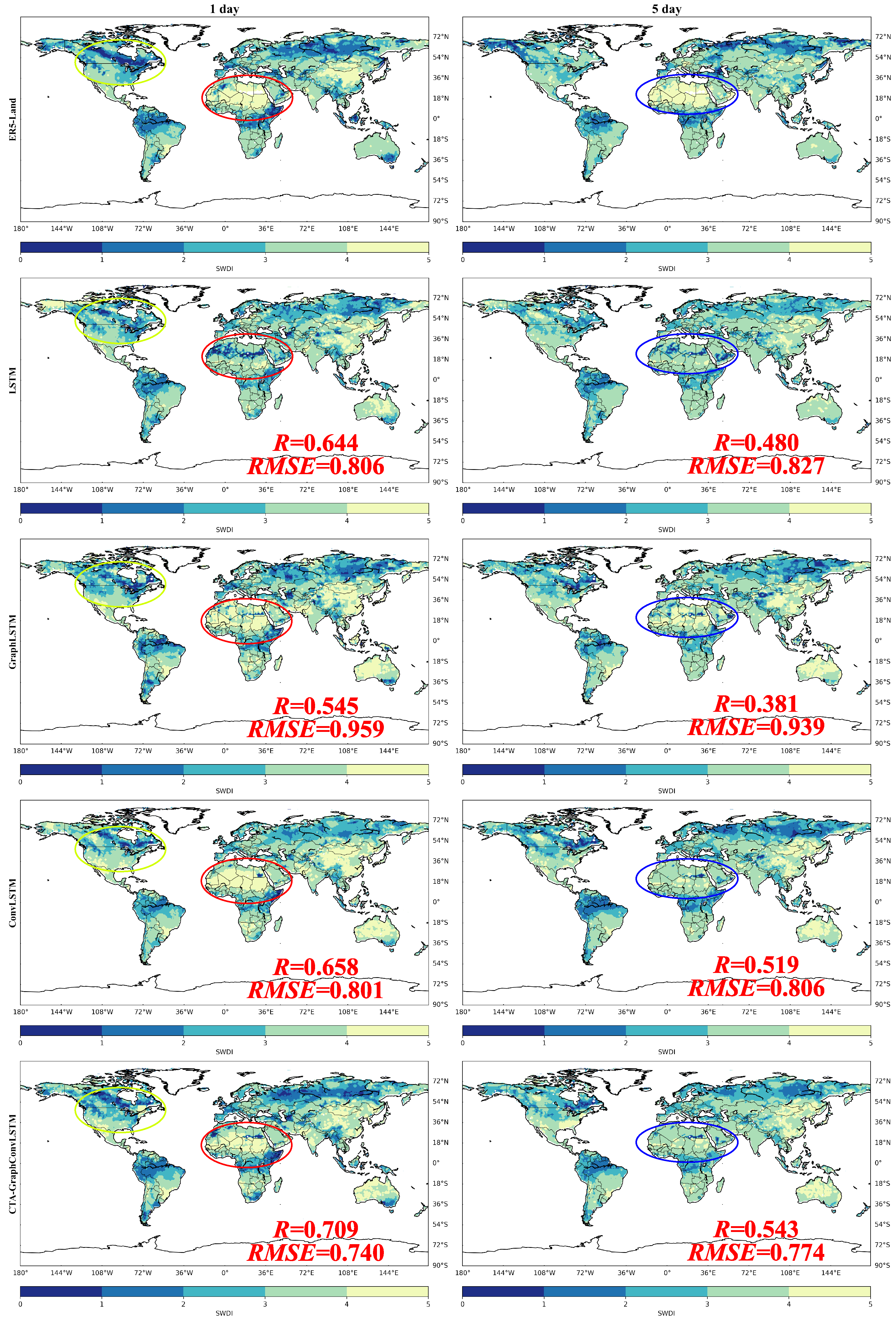
The Soil Water Deficit Index (SWDI) is used to classify drought levels, and the classification effects of each model in global drought level prediction are compared. We utilized four DL models to demonstrate the classification of drought levels across the globe using SWDI. Initially, the drought level for each day in the test set was computed based on the real data from ERA5-Land. Subsequently, the predicted values from different models were used to calculate the daily drought levels. The global drought levels predicted by the four DL models are depicted in Figure 12, while the various metrics for each model are presented in

Table 7. Evaluation metrics for 1-day ahead SWDI prediction using four deep learning models.

Model	R	${\mathit{R}}^2$	$\mathit{RMSE}$	$\mathit{ubRMSE}$	$\mathit{Bias}$	$\mathit{KGE}$
LSTM	0.664	0.223	0.806	0.720	0.512	0.356
GraphLSTM	0.545	−0.119	0.959	0.836	0.663	0.127
ConvLSTM	0.658	0.227	0.801	0.702	0.507	0.345
CTA-GraphConvLSTM	0.709	0.338	0.740	0.673	0.458	0.422

and

Table 8. Evaluation metrics for 5-day ahead SWDI prediction using four deep learning models.

Model	R	${\mathit{R}}^2$	$\mathit{RMSE}$	$\mathit{ubRMSE}$	$\mathit{Bias}$	$\mathit{KGE}$
LSTM	0.480	−0.003	0.827	0.748	0.535	0.158
GraphLSTM	0.381	−0.289	0.939	0.840	0.644	0.052
ConvLSTM	0.519	0.031	0.806	0.738	0.515	0.182
CTA-GraphConvLSTM	0.543	0.113	0.774	0.718	0.479	0.203

. It should be noted that negative $R^2$ values appear for the GraphLSTM model in both tables. Statistically, this means the prediction error of GraphLSTM exceeds the overall variation of the observed SWDI, and its drought forecasting performance is even worse than a naive mean-based baseline.

The comparison of predicted results from the graph illustrates the most significant differences in the forecasted results, particularly in the northern parts of Africa, as indicated by the red ellipse. In this region, the computation of the ERA5 real values indicates a vast area of drought, with only a small portion (the upper-left part) characterized as moist areas. The four models display distinct outcomes in this area. The LSTM model predicts most of this area as moist, which significantly differs from the actual values. The GraphLSTM shows slightly better results than LSTM for this area, yet it still fails to predict the extensive drought condition accurately. ConvLSTM captures the vast drought conditions in this area, exhibiting the best performance. However, it did not precisely forecast the slightly moist part in the upper-left region. Conversely, GraphConvLSTM slightly underperformed compared to ConvLSTM in predicting drought for this area, but it accurately forecasted the moist conditions in the upper-left part. Similar instances occurred within the yellow ellipse, where most of the area was expected to be moist. Observing the four models, GraphConvLSTM captured the extremely moist conditions within this area. However, when the prediction spanned five days ahead, as seen in the blue ellipse, the four DL models failed to predict the area’s extreme drought condition. The models’ ability to forecast drought levels significantly weakened, especially in cases of extreme drought. In summary, based on the drought level comparisons among the four models and the comparison of their R and RMSE values, our proposed GraphConvLSTM model demonstrated outstanding performance. This underlines the widespread applicability of our proposed model in predicting global drought levels.

3.5. Ablation Study of Core Modules

To verify the effectiveness of the three core modules: graph convolution (GCN), SENet channel attention, and 3D-SENet temporal attention, an ablation experiment is designed in this paper. The backbone network and training parameters of the model remain completely unchanged, and only one module is removed for each comparison experiment to evaluate the prediction performance. The detailed results are presented in

Table 9. Ablation Experimental Results of Core Modules for Soil Moisture Prediction.

Model	Module Combination	1-Day ${\mathit{R}}^2$	1-Day RMSE	5-Day ${\mathit{R}}^2$	5-Day RMSE
ConvLSTM (Baseline)	No attention, no graph convolution	0.444	0.037	0.230	0.042
CTA-ConvLSTM	Channel + Temporal Attention, w/o GCN	0.480	0.035	0.260	0.041
CTA-GraphConvLSTM w/o Temporal Attention	GCN + Channel Attention	0.500	0.034	0.270	0.040
CTA-GraphConvLSTM w/o Channel Attention	GCN + Temporal Attention	0.510	0.033	0.280	0.039
CTA-GraphConvLSTM (Full)	GCN + Channel + Temporal Attention	0.555	0.032	0.313	0.038

.

The results show that compared with the baseline ConvLSTM, the introduction of the attention mechanism or graph convolution alone can improve the prediction accuracy. When any single core module is removed, the $R^2$ values of 1-day and 5-day lead times decrease significantly and the RMSE values increase accordingly. Among them, graph convolution significantly improves the prediction accuracy of spatially heterogeneous regions; temporal attention effectively alleviates the accuracy attenuation of long lead-time prediction; channel attention optimizes the weight of input features. The synergistic effect of the three modules enables the complete CTA-GraphConvLSTM model to achieve the optimal prediction performance, which verifies the necessity and effectiveness of each module.

4. Discussion

4.1. Core Analysis of Experimental Results

Predicting soil moisture means working with high-dimensional spatiotemporal data. If you only look at time-based features, you will not obtain good results. Here, GraphLSTM tried to merge spatial and temporal information using a graph structure for graph-to-graph prediction. But its $R^2$ for a 1-day lead was just 0.088, much worse than plain LSTM. The core reason for this result is that LSTM itself is designed for sequence data with strong temporal correlation, while GraphLSTM forcibly introduces spatial features without optimizing the graph structure modeling logic, which causes the model to deviate from the core goal of temporal modeling and eventually leads to serious performance degradation.

Based on the full indicator results of Table 2 (soil moisture prediction) to Table 5 (SWDI drought level prediction), this study adopts R, $R^2$, RMSE, ubRMSE, Bias and KGE for multi-dimensional evaluation. At 1-day lead time, CTA-GraphConvLSTM achieves $R^2$ = 0.555, RMSE = 0.032, ubRMSE = 0.029, Bias = 0.023 and KGE = 0.710; at 5-day lead time, $R^2$ = 0.313, RMSE = 0.039 and KGE = 0.623, all indicators are superior to the comparative models. In SWDI drought prediction, the model also shows optimal performance with $R^2$ = 0.338, RMSE = 0.740 and KGE = 0.543 at 1-day lead time.

The adaptive graph convolution structure abandons the fixed grid adjacency and fits the real hydrological connectivity, which is the key reason for the significant performance improvement of the model in regions dominated by river and groundwater effects.

The ConvLSTM model integrates the spatial feature extraction ability of CNN and the temporal dependency modeling ability of LSTM, which can simultaneously capture the spatiotemporal variation characteristics of soil moisture. Therefore, its prediction performance is significantly better than LSTM and GraphLSTM, with an $R^2$ of 0.444 for a 1-day lead time.

The proposed CTA-GraphConvLSTM model in this study achieved the best performance among the four models, with an $R^2$ of 0.555 for 1-day lead time, which proves the feasibility and effectiveness of transforming global soil moisture prediction into an image segmentation task.

4.2. Comparative Analysis with Existing Studies

The prediction accuracy of this study shows significant performance advantages compared with existing state-of-the-art (SOTA) studies on global-scale soil moisture prediction. Ma et al. [41] conducted a systematic benchmark assessment of mainstream deep learning models on the LandBench dataset, and the optimal baseline model achieved an $R^2$ of 0.48 in the 1-day lead time global soil moisture prediction task. This comparison is implemented under fully identical dataset specifications, spatial resolution, data partitioning rules and evaluation metrics, which realizes fair and direct performance verification under consistent experimental settings. Wang et al. [10] summarized in their review that the $R^2$ of current mainstream deep learning models for global soil moisture prediction is concentrated in the range of 0.42–0.52. It is worth noting that most of the research objects summarized in this review adopt different datasets and experimental frameworks. Considering such objective heterogeneity, we unify the comparison standard focusing on global-scale short-term soil moisture prediction scenarios and mainstream hydrological evaluation indicators, so as to ensure the rationality and reference value of cross-literature comparison. The CTA-GraphConvLSTM model proposed in this study achieves an $R^2$ of 0.555 for the 1-day lead time, which is 6.7–32.1% higher than the existing SOTA models, proving the advancement of the proposed model. In the drought level prediction task, the $R^2$ of the Soil Water Deficit Index (SWDI) of the proposed model for the 1-day lead time reaches 0.338, which is 48.9% higher than the suboptimal ConvLSTM model, and the RMSE is reduced by 7.6%. This indicates that the proposed model has more prominent practical value in agricultural drought early warning scenarios and can effectively support global-scale drought monitoring and early warning.

4.3. Application Value of the Model

The CTA-GraphConvLSTM model proposed in this study has clear application value in multiple fields:

(1)

Agricultural Production: Achieve high-precision root zone soil moisture prediction and provide decision-making basis for precise irrigation and fertilization.

(2)

Water Resources Management: Support scientific allocation of watershed water resources and improve the scientificity of regional water resources management.

(3)

Ecology and Meteorology: Provide high-precision prediction data of land surface variables for weather forecasting and ecological environment assessment.

(4)

Disaster Early Warning: Provide scientific support for drought and geological disaster early warning and reduce disaster risks.

4.4. Limitation Analysis of the Model

This study still has the following limitations to be improved:

(1)

Spatial Discontinuity: The neighborhood smoothing effect of graph-to-graph prediction leads to local deviation in areas with strong soil moisture spatial heterogeneity.

(2)

Feature Modeling Limitation: Lack of global-scale feature modeling, which restricts the long-lead prediction performance.

(3)

Dataset and Validation Limitation: Only 1° resolution single-year data is adopted, lacking multi-year cross-validation and in-situ measured data verification.

(4)

Data Adaptability Limitation: Only reanalysis datasets are used, and the adaptability to multi-source remote sensing data is not verified.

4.5. Future Research Prospects

Future research will be carried out in the following directions to address the above limitations:

(1)

Optimize spatiotemporal modeling ability by introducing Transformer and solving the problem of spatial discontinuity.

(2)

Conduct multi-scale and multi-dataset verification under 0.5–4° resolutions and multi-year cross-validation.

(3)

Supplement in-situ measured data verification from global soil moisture monitoring network.

(4)

Expand the model to the prediction of land surface variables such as soil temperature and evapotranspiration.

5. Conclusions

Land big data provides rich and detailed surface information for agricultural production, ecological protection and water resources management, and supports scientific decision-making for land use and sustainable development. Deep learning can effectively model the nonlinear relationship of complex spatiotemporal land data, and accurately capture the dynamic changes of soil moisture. Aiming at the global soil moisture prediction task, this study constructs the CTA-GraphConvLSTM model integrating channel-temporal attention and graph convolution, and carries out systematic experiments on the LandBench dataset. The core conclusions are as follows:

(1)

The proposed CTA-GraphConvLSTM achieves the best performance in global soil moisture prediction. The 1-day lead time $R^2$ reaches 0.555 (25.0% higher than ConvLSTM) and the 5-day lead time $R^2$ is 0.313 (36.1% higher than ConvLSTM), with RMSE reduced to 0.032, showing stable prediction ability under different lead times.

(2)

The model has obvious advantages in drought grade prediction. The 1-day lead time $R^2$ of Soil Water Deficit Index (SWDI) is 0.338 (48.9% higher than the suboptimal model) and RMSE is reduced by 7.6%, which can provide reliable technical support for global agricultural drought monitoring and early warning.

(3)

The graph-to-graph prediction framework based on image segmentation realizes the synchronous extraction of soil moisture temporal, spatial and channel features, which solves the problem of insufficient spatiotemporal feature fusion of traditional models and is more suitable for global-scale prediction tasks.

(4)

The channel-temporal attention mechanism can adaptively enhance the key features and time steps affecting soil moisture changes, and significantly improve the model’s ability to capture extreme dry-wet events and soil moisture peak changes.

This model expands the application of graph deep learning in the field of soil moisture prediction, and provides a new technical method for drought early warning, water resources management and agricultural production decision-making. In the future, we will further optimize the global feature modeling ability of the model, carry out multi-source data verification and in-situ measured data validation, and improve the generalization performance and practical application value of the model.

References

1. Han, L.; Liu, Y.; Liu, J.; Kang, H.; Liu, Z.; Tuo, F.; Gan, S.; Ren, Y.; Yi, C.; Hu, G. Microtopography Affects the Diversity and Stability of Vegetation Communities by Regulating Soil Moisture. Water 2025, 17, 1012. [Google Scholar] [CrossRef]
2. Oyounalsoud, M.S.; Yilmaz, A.G.; Abdallah, M.; Abdeljaber, A. Drought prediction using artificial intelligence models based on climate data and soil moisture. Sci. Rep. 2024, 14, 19700. [Google Scholar] [CrossRef]
3. Nguyen, T.T.; Ngo, H.H.; Guo, W.; Chang, S.W.; Nguyen, D.D.; Nguyen, C.T.; Zhang, J.; Liang, S.; Bui, X.T.; Hoang, N.B. A low-cost approach for soil moisture prediction using multi-sensor data and machine learning algorithm. Sci. Total Environ. 2022, 833, 155066. [Google Scholar] [CrossRef]
4. Yan, S.; Weng, B.; Dong, Z.; Yan, D.; Fu, Q. Simulation of soil moisture and drought prediction in middle reaches of the Yellow River based on machine learning. Agric. Water Manag. 2026, 323, 110068. [Google Scholar] [CrossRef]
5. Reichstein, M.; Camps-Valls, G.; Stevens, B.; Jung, M.; Denzler, J.; Carvalhais, N.; Prabhat. Deep learning and process understanding for data-driven Earth system science. Nature 2019, 566, 195–204. [Google Scholar] [CrossRef] [PubMed]
6. Tuo, Y.; Wirthensohn, M.; Ma, H.; Avanzi, F. Attention-Based Graph Neural Network for Drought Forecasting: Model Performance, Stability and Interpretability. ESS Open Arch. 2025, 2025, 1–56. [Google Scholar] [CrossRef]
7. Houben, T.; Ebeling, P.; Khurana, S.; Schmid, J.S.; Boog, J. Machine-learning based spatiotemporal prediction of soil moisture in a grassland hillslope. Vadose Zone J. 2025, 24, e70011. [Google Scholar] [CrossRef]
8. Xiao, Q.; Li, Q.; Li, L.; Zhang, C.; Zhu, J.; Chen, X.; Wang, J.; Wei, S.; Wei, Z.; Dong, W.; et al. A novel diversity-aware sampling method for global soil moisture prediction. J. Hydrol. 2025, 662, 133851. [Google Scholar] [CrossRef]
9. Vahidi, M.; Shafian, S.; Frame, W.H. Multi-depth soil moisture estimation via 1D convolutional neural networks from drone-mounted ground penetrating Radar data. Comput. Electron. Agric. 2025, 232, 110104. [Google Scholar] [CrossRef]
10. Wang, Y.; Shi, L.; Hu, Y.; Hu, X.; Song, W.; Wang, L. A comprehensive study of deep learning for soil moisture prediction. Hydrol. Earth Syst. Sci. 2024, 28, 917–943. [Google Scholar] [CrossRef]
11. Hegazi, E.H.; Samak, A.A.; Yang, L.; Huang, R.; Huang, J. Prediction of Soil Moisture Content from Sentinel-2 Images Using Convolutional Neural Network (CNN). Agronomy 2023, 13, 656. [Google Scholar] [CrossRef]
12. Adeyemi, O.; Grove, I.; Peets, S.; Domun, Y.; Norton, T. Dynamic neural network modelling of soil moisture content for predictive irrigation scheduling. Sensors 2018, 18, 3408. [Google Scholar] [CrossRef]
13. Celik, M.F.; Isik, M.S.; Yuzugullu, O.; Fajraoui, N.; Erten, E. Soil Moisture Prediction from Remote Sensing Images Coupled with Climate, Soil Texture and Topography via Deep Learning. Remote Sens. 2022, 14, 5584. [Google Scholar] [CrossRef]
14. Koohikeradeh, E.; Gumiere, S.J.; Bonakdari, H. NDMI-Derived Field-Scale Soil Moisture Prediction Using ERA5 and LSTM for Precision Agriculture. Sustainability 2025, 17, 2399. [Google Scholar] [CrossRef]
15. Li, Q.; Zhao, Y.; Yu, F. A novel multichannel long short-term memory method with time series for soil temperature modeling. IEEE Access 2020, 8, 182026–182043. [Google Scholar] [CrossRef]
16. Datta, P.; Faroughi, S.A. A multihead LSTM technique for prognostic prediction of soil moisture. Geoderma 2023, 433, 116452. [Google Scholar] [CrossRef]
17. Shi, X.; Chen, Z.; Wang, H.; Yeung, D.Y.; Wong, W.K.; Woo, W.C. Convolutional LSTM network: A machine learning approach for precipitation nowcasting. Adv. Neural Inf. Process. Syst. 2015, 28, 802–810. [Google Scholar] [CrossRef]
18. Fang, W.; Pang, L.; Yi, W.; Sheng, V.S. AttEF: Convolutional LSTM Encoder-Forecaster with Attention Module for Precipitation Nowcasting. Intell. Autom. Soft Comput. 2021, 30, 453–466. [Google Scholar] [CrossRef]
19. Wu, T.; Xu, L.; Lv, Y.; Cai, R.; Pan, Z.; Zhang, X.; Zhang, X.; Chen, N. Integrating causal inference with ConvLSTM networks for spatiotemporal forecasting of root zone soil moisture. J. Hydrol. 2025, 659, 133246. [Google Scholar] [CrossRef]
20. ElSaadani, M.; Habib, E.; Abdelhameed, A.M.; Bayoumi, M. Assessment of a spatiotemporal deep learning approach for soil moisture prediction and filling the gaps in between soil moisture observations. Front. Artif. Intell. 2021, 4, 636234. [Google Scholar] [CrossRef] [PubMed]
21. Yinglan, A.; Wang, G.; Hu, P.; Lai, X.; Xue, B.; Fang, Q. Root-zone soil moisture estimation based on remote sensing data and deep learning. Environ. Res. 2022, 212, 113278. [Google Scholar] [CrossRef]
22. Habiboullah, A.; Louly, M.A. Soil Moisture Prediction Using NDVI and NSMI Satellite Data: ViT-Based Models and ConvLSTM-Based Model. SN Comput. Sci. 2023, 4, 140. [Google Scholar] [CrossRef]
23. Liang, X.; Shen, X.; Feng, J.; Lin, L.; Yan, S. Semantic object parsing with graph lstm. In Proceedings of the Computer Vision–ECCV 2016: 14th European Conference, Amsterdam, The Netherlands, 11–14 October 2016; Proceedings, Part I 14; Springer: Berlin/Heidelberg, Germany, 2016; pp. 125–143. [Google Scholar]
24. Silva, S.J.; Burrows, S.M.; Evans, M.J.; Halappanavar, M. A graph theoretical intercomparison of atmospheric chemical mechanisms. Geophys. Res. Lett. 2021, 48, e2020GL090481. [Google Scholar] [CrossRef]
25. Miao, K.; Wang, W.; Hu, R.; Zhang, L.; Zhang, Y.; Wang, X.; Nian, F. Multimodal semisupervised deep graph learning for automatic precipitation nowcasting. Math. Probl. Eng. 2020, 2020, 4018042. [Google Scholar] [CrossRef]
26. Yang, C.; Li, S.; Gou, Z. Spatiotemporal prediction of urban building rooftop photovoltaic potential based on GCN-LSTM. Energy Build. 2025, 334, 115522. [Google Scholar] [CrossRef]
27. Liao, W.; Bak-Jensen, B.; Pillai, J.R.; Yang, Z.; Liu, K. Short-term power prediction for renewable energy using hybrid graph convolutional network and long short-term memory approach. Electr. Power Syst. Res. 2022, 211, 108614. [Google Scholar] [CrossRef]
28. Vyas, A.; Shukla, A.; Kumar, A. Dynamic Structure Learning through Graph Neural Network for Forecasting Soil Moisture in Precision Agriculture. In Proceedings of the Thirty-First International Joint Conference on Artificial Intelligence (IJCAI), Vienna, Austria, 23–29 July 2022; IJCAI: Darmstadt, Germany, 2022; Volume 2022, pp. 5210–5216. [Google Scholar]
29. Azmat, M.; Madondo, M.; Bawa, A.; Dipietro, K.; Horesh, R.; Jacobs, M.; Srinivasan, R.; O’Donncha, F. Forecasting Soil Moisture Using Domain Inspired Temporal Graph Convolution Neural Networks To Guide Sustainable Crop Management. In Proceedings of the Thirty-Second International Joint Conference on Artificial Intelligence (IJCAI), Macao, China, 19–25 August 2023; IJCAI: Darmstadt, Germany, 2023; Volume 2023, pp. 5897–5905. [Google Scholar]
30. Hu, J.; Shen, L.; Sun, G. Squeeze-and-Excitation Networks. In Proceedings of the 31st IEEE/CVF Conference on Computer Vision and Pattern Recognition (CVPR), Salt Lake City, UT, USA, 18–23 June 2018; pp. 7132–7141. [Google Scholar]
31. Woo, S.; Park, J.; Lee, J.Y.; Kweon, I.S. CBAM: Convolutional block attention module. In Proceedings of the European Conference on Computer Vision (ECCV), Munich, Germany, 8–14 September 2018; Springer: Cham, Switzerland, 2018; Volume 2018, pp. 3–19. [Google Scholar]
32. Zhang, L.; Wang, H.; Li, Y. Attention-Enhanced ConvLSTM for Spatio-Temporal Soil Moisture Prediction Using Multi-Source Remote Sensing Data. Remote Sens. 2024, 16, 1324. [Google Scholar]
33. Li, Q.; Zhang, C.; Shangguan, W.; Wei, Z.; Yuan, H.; Zhu, J.; Li, X.; Li, L.; Li, G.; Liu, P.; et al. LandBench 1.0: A Benchmark Dataset and Evaluation Metrics for Data-Driven Land Surface Variables Prediction. Expert Syst. Appl. 2024, 243, 122971. [Google Scholar] [CrossRef]
34. Hochreiter, S.; Schmidhuber, J. Long Short-Term Memory. Neural Comput. 1997, 9, 1735–1780. [Google Scholar] [CrossRef]
35. Zhang, R.; Li, L.; Zhang, Y.; Huang, F.; Li, J.; Liu, W.; Mao, T.; Xiong, Z.; Shangguan, W. Assessment of Agricultural Drought Using Soil Water Deficit Index Based on ERA5-Land Soil Moisture Data in Four Southern Provinces of China. Agriculture 2021, 11, 411. [Google Scholar] [CrossRef]
36. Pablos, M.; Martinez-Fernandez, J.; Sanchez, N.; Gonzalez-Zamora, A. Temporal and Spatial Comparison of Agricultural Drought Indices from Moderate Resolution Satellite Soil Moisture Data over Northwest Spain. Remote Sens. 2017, 9, 1168. [Google Scholar] [CrossRef]
37. Xu, Z.-g.; Wu, Z.-y.; He, H.; Guo, X.; Zhang, Y.-l. Comparison of soil moisture at different depths for drought monitoring based on improved soil moisture anomaly percentage index. Water Sci. Eng. 2021, 14, 171–183. [Google Scholar] [CrossRef]
38. Liu, Y.; Shi, L.; Wang, Y. Enhancing data-driven soil moisture modeling with physically-guided LSTM networks. Front. For. Glob. Chang. 2025, 8, 1353011. [Google Scholar]
39. Pan, Z.; Xu, L.; Chen, N. Combining graph neural network and convolutional LSTM network for multistep soil moisture spatiotemporal prediction. J. Hydrol. 2024, 633, 132572. [Google Scholar] [CrossRef]
40. Xi, X.; Zhuang, Q.; Liu, X. A Hybrid Physics-Guided Deep Learning Modeling Framework for Predicting Surface Soil Moisture. J. Geophys. Res. Mach. Learn. Comput. 2025, 2, e2025JH000682. [Google Scholar] [CrossRef]
41. Zhang, R.; Li, S.; Zhou, J.; Wu, H.; Huang, G. A hybrid attention-enhanced graph convolutional network for global surface soil moisture prediction. Agric. Water Manag. 2025, 301, 109268. [Google Scholar] [CrossRef]
Figure 1. Framework diagram of 3D-SENet.
Water 18 01308 g001
Figure 2. The description of SENet.
Water 18 01308 g002
Figure 3. The architecture of CTA-GraphConvLSTM.
Water 18 01308 g003
Figure 4. Flow chart of the overall research method for the CTA-GraphConvLSTM model.
Water 18 01308 g004
Figure 5. The box plots for LSTM, GraphLSTM, ConvLSTM, and CTA-GraphConvLSTM with a temporal window of 7 and a prediction horizon of 1 are presented below.
Water 18 01308 g005
Figure 6. Correlation heatmap between input variables and soil moisture.
Water 18 01308 g006
Figure 7. R 2 values of four deep learning models for 1-day ahead soil moisture prediction over six global geographical regions (sorted by arid to humid: North Africa, NW USA, Southern Africa, SE USA, South China, Northern Brazil).
Water 18 01308 g007
Figure 8. Spatial distribution of R 2 for the four deep learning models at 1-day lead time for soil moisture prediction. White areas indicate R 2 < 0, meaning that the model’s predictions are worse than simply using the historical mean. For regions with R 2 ≥ 0, a continuous color gradient from blue to red is used, where blue represents low R 2 (poor but still positive performance) and red represents high R 2 (good performance).
Water 18 01308 g008
Figure 9. ERA5-Land’s global soil moisture ( m 3 / m 3 ) and the predictions made by LSTM, GraphLSTM, ConvLSTM, and CTA-GraphConvLSTM models at a 1-degree resolution. The top row illustrates the ‘true’ ERA5-Land field for the 1st layer (0–7 cm) with predictions made for 1 day and 5 days in advance. The subsequent prediction models are LSTM (2nd row), GraphLSTM (3rd row), ConvLSTM (4th row), and CTA-GraphConvLSTM (bottom row). Please note that the results are validated using data from a random day in 2020 (the 121st day).
Water 18 01308 g009
Figure 10. Different deep learning prediction models for soil moisture are evaluated based on R M S E , R, and B i a s , considering a 1-degree spatial resolution and a 1-day lead time. The results for the four distinct DL models are presented in different rows, with R M S E on the left, R values in the middle column, and B i a s values on the right. The time step and prediction time for all four models are consistent, set at 7 days and 1 day.
Water 18 01308 g010
Figure 11. A global map featuring randomly selected grid points and a time series of soil moisture for different grid points is depicted. The five time-series subplots from top to bottom are labeled as (ae), which correspond to the blue, red, green, yellow, and black five-pointed stars on the global map, respectively. These time series were generated using models with a 7-time step length, specifically CTA-GraphConvLSTM and ConvLSTM, for a 1-day lead time.
Water 18 01308 g011
Figure 12. SWDI calculated from global soil moisture of ERA5-Land and SWDI derived from predictions of LSTM, GraphLSTM, ConvLSTM, and GraphConvLSTM models (1-degree resolution).
Water 18 01308 g012