Article

Near-Future Climate Change Impacts on Sado River (Southern Portugal) Flow Rates Using CMIP6-HSPF Modelling


1
Centre for the Research and Technology of Agro-Environmental and Biological Sciences (CITAB), University of Trás-os-Montes e Alto Douro (UTAD), 5000-801 Vila Real, Portugal
2
Institute for Innovation, Capacity Building and Sustainability of Agri-Food Production (Inov4Agro), 5000-801 Vila Real, Portugal
3
Potsdam Institute for Climate Impact Research (PIK), Member of the Leibniz Association, 14412 Potsdam, Germany
4
Institute of Environmental Science and Geography, University of Potsdam, 14476 Potsdam, Germany
5
BIORG—Bioengineering and Sustainability Research Group, Faculty of Engineering, Lusófona University, 1749-024 Lisbon, Portugal
6
LEAF—Linking Landscape, Environment, Agriculture and Food, Instituto Superior de Agronomia, Universidade de Lisboa, Tapada da Ajuda, 1349-017 Lisbon, Portugal
*
Author to whom correspondence should be addressed.
Water 2026, 18(4), 442; https://doi.org/10.3390/w18040442
Submission received: 5 January 2026 / Revised: 2 February 2026 / Accepted: 5 February 2026 / Published: 7 February 2026

Abstract

Climate change impacts on the Sado River (southwest Portugal) flow rates (FRs) were assessed for the first time under the 2041–2060 Shared Socioeconomic Pathways: 1–2.6 W/m2 (SSP1-2.6), 3–7.0 W/m2 (SSP3-7.0), and 5–8.5 W/m2 (SSP5-8.5), using bias-adjusted and downscaled General Circulation Model (GCM) ensemble projections from the Inter-Sectoral Impact Model Intercomparison Project (ISIMIP3b-Sado). ISIMIP3b-Sado was used to estimate future precipitation and temperature changes, and as input for Hydrological Simulation Program—FORTRAN (HSPF) simulations. The HSPF projected decreases in the Sado FRs, mainly under SSP3-7.0 and SSP5-8.5, due to temperature increases and autumn/spring precipitation decreases. The FR decreases may lead to 29%/33% reductions in yearly accumulated riverine water volume under SSP3-7.0/SSP5-8.5 and a 31% summertime riverine water deficit increase under SSP3-7.0. Surface-water demand fulfilment in the Sado Basin could suffer a 22-day delay, and the wintertime precipitation range is projected to increase. Hence, in the near-future, summertime surface-water needs and reservoir recharge in the Sado Basin could become more dependent on wintertime precipitation. With Sado being an agricultural region, our results should prompt agriculture stakeholders and decision makers to improve wintertime surface water storage and management to sustain summertime crop irrigation needs.

1. Introduction

Water is one of Earth’s most used resources and is consumed abundantly by economic sectors such as agriculture. During 2022, total annual water abstraction in the European Union (EU) reached 197   ×   10 9   m 3 [1]. The majority of it was used for electricity cooling, accounting for 34% of the abstractions, followed by the agriculture sector, at 29% [1]. However, since the agri-food industry accounts for approximately 30% of the world’s total energy consumption, it is clear that agriculture is, overall, the EU’s biggest water-abstracting economic sector [2]. Agriculture is a highly seasonal activity, especially in Southern Europe, where crops are typically grown during spring and summer. These are the seasons when surface water availability has been decreasing, due to a combination of socioeconomic and climate changes, such as increased agricultural water demand, increasing temperatures, and more frequent and intense droughts and heat waves [1]. As a result, between 2000 and 2023, surface water abstraction by European farmers has decreased by 13% [1]. Given the rising agricultural water demand and the major socioeconomic importance of agriculture, a shift to groundwater abstraction occurred during the same period, which led to groundwater abstraction increasing by 52% [1].
Within Southern Europe, the southern Iberian Peninsula (IP) has been one of the regions most impacted by climate change. This is already a predominantly arid region, where droughts occur three times per decade and typically last between two and three years [3]. However, increases in the frequency, intensity, and duration of drought events throughout the 20th and early 21st centuries, along with drying trends identified during the same period, reveal that the southern IP climate could become even more arid, though similar results were obtained for other regions in Southern Europe [4,5,6,7]. This is also the conclusion of future-climate projection studies, which project more severe and longer drought events, ten times more frequent heatwaves, and 15% less seasonal precipitation [8,9,10]. The expected aridification of the southern IP territory could increase the risk of surface water scarcity throughout the 21st century [11]. Mean annual runoff projections for the southern Spanish river basins for 2070–2100 under the Representative Concentration Pathways (RCP) anthropogenic forcing scenarios indicated that runoff could decrease between 17% and 20% under RCP4.5, and between 29% and 38% under RCP8.5 [12]. The projected decreases in runoff could not only impact the recharge of the basin’s surface water reservoirs, but also the recharge of neighbouring basins, through reductions in water transfers. In the case of the Tagus River Basin (central Spain), hydrological model projections for 2020–2090 pointed towards a water resources decrease of 40% under RCP4.5 and 47% under RCP8.5 [13]. This decrease could lead to a 70% to 79% reduction in water transfers from the Tagus to the Segura River Basin (southeast Spain) during the same period, under both RCP scenarios.
Studies on the impacts of future climate and socioeconomic changes on the southern Spanish surface water reserves are vast, yet similar studies on the southern Portuguese surface water reserves are scarce in comparison and generally conducted at a smaller, subbasin scale. Therefore, little information is available regarding the impact on the surface water reserves of larger southern Portuguese basins and the subsequent impact on the region’s agriculture sector. One such example is the Sado River Basin (hereafter SRB), one of the largest Portuguese catchments and home to important agricultural hubs [14]. Within the few studies available for this basin, projections for the “Vale do Gaio” reservoir (northern half of the basin) have shown that, for 2071–2100, reservoir inflows could decrease between 19% and 23% under the Special Report on Emissions (SRES) A1B and B1 future socioeconomic scenarios [15]. Similar conclusions were found by another study, which stated that by the end of the 21st century, both the SRB and the neighbouring Guadiana River Basin could experience a 50% runoff loss during spring and autumn, and a 10% runoff loss during winter, under the SRES A2 scenario [16]. These findings are especially relevant, given that the SRB receives water transfers from the Alqueva reservoir, located in the Guadiana River Basin, when its endogenous water resources become insufficient to support local demand.
Similar to the Spanish surface water reserves, these studies have shown that recharging the Sado River might become increasingly more challenging in the coming decades, whether with endogenous or transferred surface water resources, since the surface reservoirs of the neighbouring basins would not be able to satisfy the surface water demands of both basins. Therefore, surface-water transfers should not be considered when assessing the climate change impacts on the SRB’s surface water. Moreover, the aforementioned studies assessed climate change impacts on basin flows for only some of the Sado subbasins at the end of the century, using decades-old climate models and scenarios. This is a severe limitation for farmers, who need state-of-the-art data over the entire SRB and near-future time periods to develop and implement efficient crop water management plans. Hence, the present study aims to project climate change impacts on near-future Sado River flow rates and surface-water volumes by performing hydrological model simulations of the SRB using the latest generation of future-climate datasets and socioeconomic scenarios.

2. Data and Methodology

2.1. Study Area Characterisation

The SRB is a watershed located in Southwest Portugal, as shown in Figure 1a. With a total area of 6529 km2, its main river, the Sado, runs along 180 km from a spring at an altitude of 230 m in “Serra da Vigia” (southern part of the basin), to its estuary located northwest of the basin, before entering the North Atlantic Ocean [14]. It is part of the Sado and Mira Hydrographic Region (RH6), a Portuguese Environmental Agency (APA) administrative region that merges the Sado and Mira River basins and is home to approximately 300,000 people (3% of the Portuguese population) [17]. The majority of the population lives within the SRB, with approximately 60% of the RH6 population living in the Setúbal district, which encompasses most of the basin’s area [18]. The SRB hosts several industrial hubs and one of the country’s most important shipping ports [19,20]. Yet, it is the agroforestry sector that has the biggest share in the local economy, with crops such as rice being predominant in the estuary and lower riverbanks, and extensive forestry (e.g., cork oak and pine trees) dominating the higher elevation areas [21]. A hypsometric chart of the basin is presented in Figure 1b, along with its water channels. The hypsometric chart is based on data from the 25 m resolution European Digital Elevation Model version 1.1 (EU-DEM), whereas the river chart was obtained from the Portuguese Environmental Information System [22,23]. As the map shows, this watershed has a relatively flat topography, with an elevation below 200 m in most of the catchment and only surpassing 300 m in its northeast border.
Since it is located in Southern Portugal, the climate of the SRB is characterised by hot dry summers and mild wet winters, thus being considered a Mediterranean climate of Csa type, following the Köppen–Geiger climate classification system [24,25,26]. Dry periods may last up to five consecutive months, and around 20% of the basin’s total annual precipitation is due to extreme precipitation events [27]. According to the 1991–2020 climatological normals from the Portuguese Weather Service (Instituto Português do Mar e da Atmosfera, IPMA), gathered from 4 weather stations surrounding the SRB (Setúbal, Alcácer do Sal, Beja, and Alvalade), this catchment receives a mean total annual precipitation amount of approximately 572 mm, while the mean annual temperature is approximately 17 °C [28]. Most of the precipitation occurs during the autumn (September–October–November) and winter (December–January–February) months, when total seasonal precipitation reaches around 200 mm. Summer (June–July–August) conditions are predominantly dry, with climatological precipitation totals of approximately 16 mm [28]. This combination of dry climate, flat topography, and precipitation seasonality makes the SRB one of Portugal’s driest, and leads to a river flow concentration during winter [29,30].
Moreover, total surface water abstractions in the SRB amounted to approximately 242 hm3/year in 2018, according to the River Basin Management Plans (RBMP) from the Portuguese Environmental Agency (APA) [31]. This estimate combined water abstractions for public water supply, human consumption, industrial use, crop and golf course irrigation, livestock farming and other uses. Nevertheless, more than 80% of the total abstracted volume was destined for crop irrigation [31]. Furthermore, surface water abstractions in the SRB exceed groundwater abstractions, which amounted to approximately 180 hm3/year in 2018 [31]. This vast water consumption is putting pressure on the water availability of a region that has experienced declining annual precipitation over the last century, and whose water recharge is projected to decline in the coming decades [27].

2.2. Climate Data

Before simulating the near-future hydrology of the SRB, simulated 2041–2060 climate data from this region were processed and compared with simulated data from a 1995–2014 reference period. The future and reference climate datasets used in this study have their origins in the simulation of three Shared Socioeconomic Pathways (SSPs) scenarios and one baseline scenario, respectively, with nine General Circulation Models (GCMs), which are described in Table 1. These GCMs were chosen due to being state-of-the-art models which have different representations of the Earth system and cover a broad set of physical and biogeochemical processes. Moreover, they were developed under the 6th phase of the Coupled Model Intercomparison Project (CMIP6), and therefore, they were developed under common standards and benchmarked against hundreds of GCMs under common experiments [32,33].
The SSP scenarios were developed for the Intergovernmental Panel on Climate Change (IPCC) 6th Assessment Report (AR6), and associate possible future socioeconomic trajectories and climate policies with changes in the radiative forcing, thus allowing for more holistic projections about the future state of the climate and its uncertainties [43]. The three SSP scenarios used were SSP1-2.6, SSP3-7.0, and SSP5-8.5, and each represents an increased human-driven radiative forcing of 2.6 W/m2, 7.0 W/m2, and 8.5 W/m2, respectively, by 2100. To allow for future regional climate impact assessments, each of the CMIP6 GCM simulations was downscaled and bias-adjusted by the Inter-Sectoral Impact Model Intercomparison Project (ISIMIP), following its 3b protocol (ISIMIP3b) [44,45,46]. Downscaling was made to a 50 km spatial resolution, and the GCM outputs were bias-adjusted towards the W5E5 reanalysis dataset [47]. This made the ISIMIP3b outputs the ideal dataset to study the SRB’s future climate, yet they still needed to be downscaled to the basin’s scale. Hence, the ISIMIP3b outputs from each GCM were further downscaled by the authors to a 30 arc-sec resolution (1 km spatial resolution) over Portugal, using the Climatologies at High resolution for the Earth’s Land Surface Areas (CHELSA) approach [48]. Then, a basin-scale bias adjustment was performed on the daily total precipitation (RR), 2-metre daily mean temperature (TG), and 2-metre daily maximum (TX) and minimum (TN) temperature datasets. Bias adjustment of model data is a widespread methodological approach that ensures adherence of simulated data to observed conditions [49,50]. In this study, the bias adjustment consisted of matching the cumulative distribution functions (CDFs) of the CHELSA-downscaled ISIMIP3b datasets with the CDFs of ERA5-Iberia, a 10 km-resolution ERA5-Land reanalysis dataset previously bias-adjusted using the Iberia01 observed weather data [27,51,52]. The used CDF matching method was developed by Miao et al. [53], as a combination of the equiratio and equidistant CDF matching methods developed by Wang et al. [54] and Li et al. [55], respectively. This method is described in Equations (1)–(3):
I ( x )   = x f ( x r x o )  
G ( x ) = x f ( x o x r )
x B C = { I ( x ) ,                     I ( x ) > 0 G ( x ) ,                 I ( x ) < 0 0 ,                               I ( x ) = 0  
where x f , x r , x o , and x B C represent the 2041–2060 ISIMIP3b data quantiles, 1995–2014 ISIMIP3b data quantiles, 1995–2014 ERA5-Iberia data quantiles, and the bias-adjusted data quantiles, respectively. All equations were applied to RR, while for TG, TX, and TN, only Equation (1) was used. Due to the lower spatial resolution of ERA5-Iberia, the CHELSA-downscaled ISIMIP3b data needed to be resampled to a 10 km spatial resolution before the bias adjustment, using a first-order conservative remapping. The results of this sequence of downscaling and bias adjustment procedures, summarised in Figure S1 (Supplementary Materials), were 36 highly statistically modified 10 km datasets, hereafter referred to as ISIMIP3b-Sado. The 36 datasets correspond to each of the nine GCMs, one reference climate period, and three future SSP scenarios. From each dataset, RR, TG, TX, TN, and surface downward shortwave radiation (RSDS) data were used as inputs to the hydrological model simulations. The bias-adjusted data variability (inter-model) is reported in the Supplementary Materials, regarding the daily TG and RR data for each season and scenario.

2.3. HSPF Model Simulations

Hydrological simulations of the SRB were made using the Hydrological Simulation Program—FORTRAN (HSPF) hydrological model. HSPF is a modelling framework developed by the United States Environmental Protection Agency (US EPA) for watershed hydrology and water quality modelling [56]. It is based on the Stanford Watershed Model IV and integrates three previously existing models, namely the Agricultural Runoff Management Model (ARM), the Nonpoint Source Runoff Model (NPS), and the Hydrological Simulation Program (HSP) [57,58,59]. The integration of these models allows for the simulation of flow rate and runoff, as well as sediment, nutrient, and contaminant concentrations, at any point in a watershed. HSPF is a semi-distributed model, meaning that it considers the spatial variability of properties such as land use, soil type, and slope [60]. Typically, semi-distributed and fully distributed hydrological models group areas with similar physical properties into Hydrological Response Units (HRUs). HRUs work as the core modelling element where all hydrological processes are computed, and the movement of water and contaminants is reproduced throughout them. However, HSPF divides the watershed into pervious (PERLND) and impervious (IMPLND) land segments, over which subbasins and reaches are superimposed by a digital elevation model (DEM) [56,60]. Hence, each subbasin in HSPF is composed of several PERLND and IMPLND, where different hydrological processes are computed, and whose flows are routed to the nearest reach. Then, the flows from each reach are routed to the subbasin’s main reach, and subsequently to the downstream reaches, by storage routing (kinematic wave) methods [61]. This modelling approach makes each subbasin effectively an HRU, and comes as an advantage over other hydrological models, since it allows for uniform meteorological inputs to the subbasin. The HSPF hydrological model runs inside the Better Assessment Science Integrating Point and Nonpoint Sources (BASINS) framework, a geographical information system (GIS) specifically developed by the US EPA for water quantity and quality modelling applications [62]. For this research, the software BASINS 4 and HSPF v12.2 were used.
The parameterisation of the HSPF model for the SRB started with its delineation in BASINS, in which subbasins and water channels were represented according to the 25 m resolution EU-DEM [23]. Due to a lack of data regarding all reservoirs’ discharges and volumes, it was decided to exclude the Sado reservoirs from the model. Soil data from the Harmonised World Soil Database v2.0 (HWSD) and land use data from the Portuguese General-Directorate of Territory were also fed into BASINS [63,64]. Then, meteorological data were input at the centroid coordinates of each subbasin. The result was a model with 17 subbasins, as shown in Figure 1b, that represents the SRB in its natural form, before the implementation of any of the existing dams and reservoirs. This allows for the simulation of the response of the basin itself to the projected climate changes, such as its riverine water volume downstream of the current artificial reservoirs, especially in the Sado River mouth. After the basin was set up in BASINS, the calibration and validation procedures were initiated. For that purpose, observed flow rates (FR hereafter) from the Sado River were then obtained from the Portuguese Hydrological Resources National Information System (SNIRH), managed by APA. The model calibration was based on the “Moinho da Gamitinha” (MG hereafter) hydrometric station, located at 38.063° N and −8.404° E (Figure 1b).
The reason for only using MG for model calibration is that it is the only SNIRH station located at the main Sado channel with observed FR data available for the 1995–2014 reference period. Nevertheless, MG covers 42% of the basin’s area, and the behaviour of the PERLND and IMPLND land segments in the MG’s subbasin is similar to that of the other PERLNDs and IMPLNDs in the basin. Furthermore, most of the basin’s area presents a flat topography. Thus, the parameterisation applied at MG is valid for the majority of the basin. An additional challenge was brought by missing data periods in the MG time series, and the quality of the data, considering that in several years, there was a low correlation between precipitation and river discharge events. Hence, the observed FR data periods adequate for model calibration and validation were very limited, which made multi-year calibration quite difficult. To overcome this issue, HSPF was manually calibrated over the years with a high correlation between observed FR and 7-day accumulated RR, reduced missing data, and different RR and FR regimes, to represent different climatic periods. For model calibration, the 2002 and 2003 years were chosen to represent an above-average annual precipitation regime. Then, to validate the calibration, the chosen years were 2018 and 2021, since annual precipitation in these years was below the average for the region. It should be mentioned that the SRB’s morphology did not suffer any modifications between the calibration and validation years, and thus, no changes to the model’s DEM were required.
For the calibration and validation simulations, a combination of SNIRH observational data and ERA5-Iberia reanalysis data from the 2001–2022 period was used, with daily RR, TX, and TN data coming from ERA5-Iberia, and daily RSDS coming from the “Viana do Alentejo” and “Moinhola” SNIRH meteorological stations (Figure 1b). Despite only needing the 2002, 2003, 2018, and 2021 time series, the time series from 2001 were necessary for a 1-year model warm-up period. To be input to HSPF, the data needed to be previously prepared in BASINS using the Watershed Data Management Utility (WDMUtil) tool [65]. WDMUtil disaggregates the daily time series into hourly time series, converts their units from the International System of Units (SI) to the United States Customary System, and calculates daily and hourly potential evapotranspiration using TX, TN, and RSDS [65]. With the data preparation concluded, the first HSPF simulations for the calibration and validation years were made. Each of these simulations required the use of different parameterisations to find the most suitable parameter values for the observed flow regime in the Sado River. Due to the large amount of missing data days, the evaluation of each parameterisation’s performance was carried out at a monthly scale, using the Nash–Sutcliffe model efficiency coefficient (NSE) [66], the coefficient of determination (R2) [67], and the percentage bias between the simulated and observed river FR (PBIAS) [68]. The NSE assesses the model performance relative to the mean observed values on a scale from −∞ to 1, where −∞, 0 and 1 indicate that the model has, respectively, a very poor, sufficient, and very good performance [66]. The coefficients are described in Equations (4), (5), and (6), respectively:
NSE   =   1 t = 1 T ( Q o t Q s t ) 2 t = 1 T ( Q o t Q o ¯ ) 2
R 2 = ( t = 1 T ( Q o t Q o ¯ ) ( Q s t Q s ¯ ) t = 1 T ( Q o t Q o ¯ ) 2 t = 1 T ( Q s t Q s ¯ ) 2 ) 2
PBIAS = t = 1 T ( Q s t Q o t ) t = 1 T Q o t 100
where t is the timestep in months, T is the studied time period in months (24 months for the calibration years, and 12 months for each validation year), Q 0 is the monthly mean observed FR, Q 0 ¯ is the annual mean observed FR, Q S is the monthly mean simulated FR, and Q s ¯ is the annual mean simulated FR. After several model runs, an optimal model parameterisation was found. As Table 2 shows, parameterisation was made at monthly and yearly scales. The possibility of monthly scale calibration given by HSPF is quite useful in the SRB, considering the accentuated differences between wintertime and summertime precipitation regimes in this region. Parameters such as the interception storage capacity (INT) and lower zone evapotranspiration (LZE) of the soil required monthly parameterisation, while at the yearly scale, adjustments were made for the lower (LZSN) and upper (UZSN) zone nominal storage; the length (LSUR), slope (SLSUR) and Manning number (NSUR) of the overland flow plain; interflow inflow parameter (INTFW); infiltration capacity of the soil (INFILT); interception storage capacity (CEPSC); and groundwater recession rate (AGWRC). Along with the model parameters, adjustments to the imperviousness percentages of the different land use groups were also made. With calibration and validation completed, HSPF simulations using the ISIMIP3b-Sado daily RR, RSDS, TX, and TN data were initiated for the 1994–2014 historical period and the three 2040–2060 SSP forcing scenarios. Like the calibration and validation simulations, the 1994 and 2040 years were used as warm-up periods. In total, 36 simulations were made with HSPF, each corresponding to a different GCM and scenario.
From each simulation, daily FR outputs were extracted, and their 20-year ensemble-pool variability was subsequently analysed at each season and scenario, using the MATLAB R2023a 9.14.0 software [69]. The same analysis was made for RR and TG. Moreover, the 20-year median GCM-ensemble yearly accumulated riverine water volume was estimated and compared with the total yearly water abstractions at the SRB, to assess future changes in the basin’s riverine water availability. Along with these analyses, the future-historical spatial changes in the 20-year mean RR, TX, TN, TG, and percentage of 20-year total RR above the historical period’s 20-year total RR 95th percentile (P95TOT) in the ISIMIP3b-Sado dataset were also analysed.

3. Results

3.1. HSPF Model Performance

The chosen parameterisation led to a good performance by HSPF in the calibration and validation years. As can be seen in Table 3, during the calibration years, mean total annual precipitation reached 597 mm, thus being slightly above the 30-year mean annual precipitation of 572 mm for the Sado region. During the 2018 and 2021 validation years, annual precipitations were 42% and 15%, respectively, below the 30-year mean. Moreover, Pearson correlation coefficients (r) of approximately 0.5, 0.7, and 0.6 were found between the observed FR at MG and the 7-day accumulated precipitation in the basin during 2002–2003, 2018, and 2021, respectively, as shown in Figure S2.
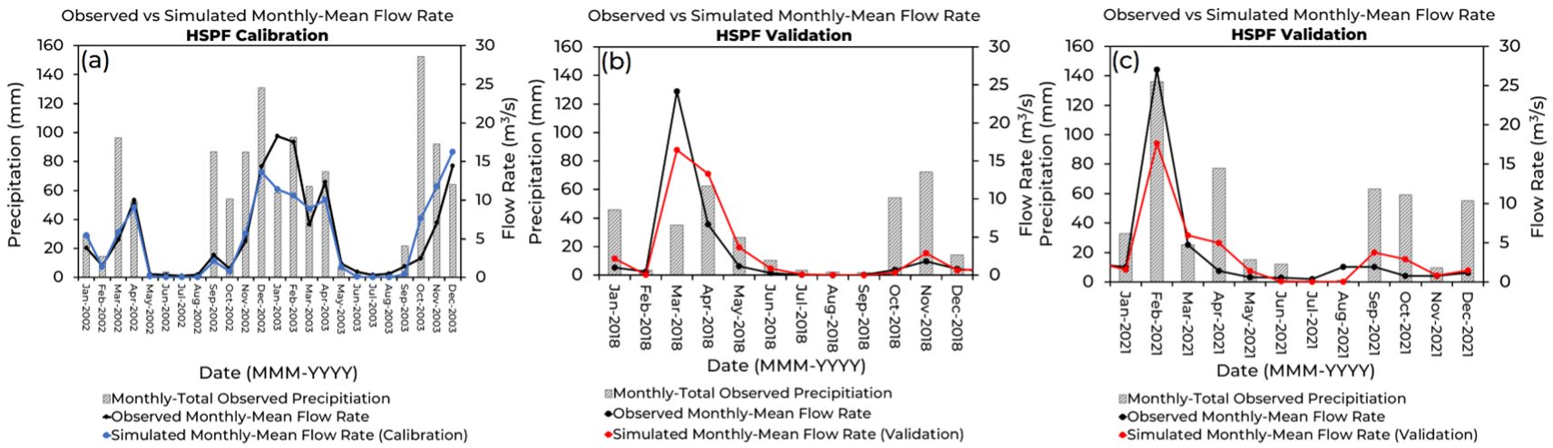
The differences between the calibration and validation years are also noticeable in the annual-mean FR, since in both the observed and simulated datasets, the annual-mean FR is above 5 m3/s during the calibration years, and between 3.1 and 3.6 m3/s during validation years. Despite these differences, HSPF displayed NSE and R2 values of approximately 0.8 and absolute PBIAS below 10% in all the calibration and validation years. These performance metrics demonstrate that the simulated FR is very similar to the observed FR registered at MG, something that can also be seen by visually comparing the simulated and observed monthly mean FR time series (Figure 2). Additionally, a comparison between the monthly mean simulated FR and the monthly total RR revealed that HSPF can accurately simulate the basin’s response to precipitation events. Hence, given the good multi-year performance of HSPF in different precipitation regimes, the model was considered calibrated and validated. Regarding the GCM ensemble variability, as can be seen in Figures S3–S8 (Supplementary Materials), the ensemble presents a homogeneous range in both RR and TG under all seasons and scenarios.

3.2. Climate Characterisation and Future Projections for the Sado River Basin

After the HSPF calibration was concluded, an analysis of the ISIMIP3b-Sado TX, TN, TG (Figure 3), annual RR (Figure 4), P95TOT (Figure 5), and seasonal RR (Figure 6) projections was conducted.
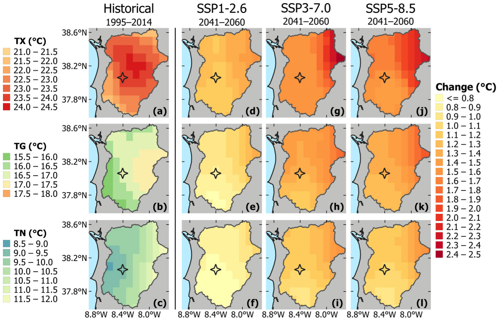
Starting with the 20-year mean daily TX, TN, and TG in the SRB during the 1995–2014 reference climate period (Figure 3a–c), the dataset shows that the spatially lowest 20-year mean TN during the historical period was approximately 9 °C (Figure 3c), and that the spatially highest 20-year mean TX was approximately 24 °C (Figure 3a). As for TG, its spatial variation was between 15 °C and 18 °C (Figure 3b). Considering the temperature spatial distribution, it is apparent that there is an inland temperature gradient, whereas, in the case of TX, it is also noticeable that the highest values are concentrated at the centre of the basin. During the 2041–2060 period, temperature increases in each scenario. The changes are expected to be higher for TX (Figure 3d,g,j) and lower for TN (Figure 3f,i,l). Spatially, the increases are projected to be higher in the northern and northeastern areas. The dataset also indicates that, overall, SSP3-7.0 is the scenario with the highest temperature changes (Figure 3g–i), except in the eastern areas of the basin, where TG and TX changes are greater under SSP5-8.5. Overall temperature changes range from 0.8 °C in TN, under SSP1-2.6, to 2.5 °C in TX, under SSP3-7.0. Hence, under these scenarios, the highest temperatures are expected to be found in the inner northern areas, and the lowest temperatures in the south–southwestern areas.
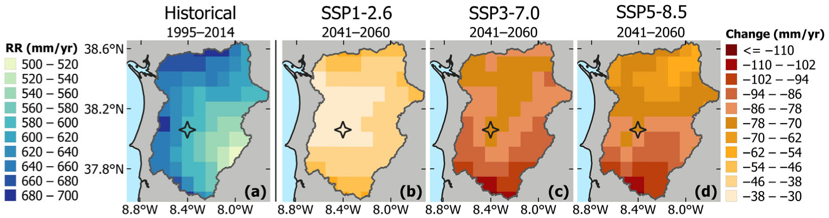
The 20-year mean total annual RR data (Figure 4a) during 1995–2014 reveal a southeast to northwest precipitation gradient. The highest RR values, ranging from approximately 640 to 700 mm/year, are found around the higher-elevation areas in the north and southwest of the basin, closely located to the coast. The lowest RR values, between roughly 500 and 560 mm/year, are found above the southeast areas of the basin, i.e., farther away from the coast.
Regarding the 2041–2060 period, annual RR projections (Figure 4b–d) show that RR could decrease under all SSP scenarios, and that the changes tend to be larger in the southern areas. SSP1-2.6 RR changes vary from −30 to −38 mm/year in the central areas, and from −38 to −62 mm/year in the northern and southern areas. As for SSP5-8.5 changes, they vary from −54 to −78 mm/year in the northern part of the basin, and from −78 to −110 mm/year in the southern part. The highest annual RR changes are found in the SSP3-7.0 scenario, where they range from −70 to −86 mm/year in the northern lower elevation areas, and from −86 to −110 mm/year in the southern higher elevation areas. Therefore, the spatial distribution of RR is projected to remain nearly invariant under SSP1-2.6, while the north–south gradient is projected to strengthen under SSP3-7.0 and SSP5-8.5.
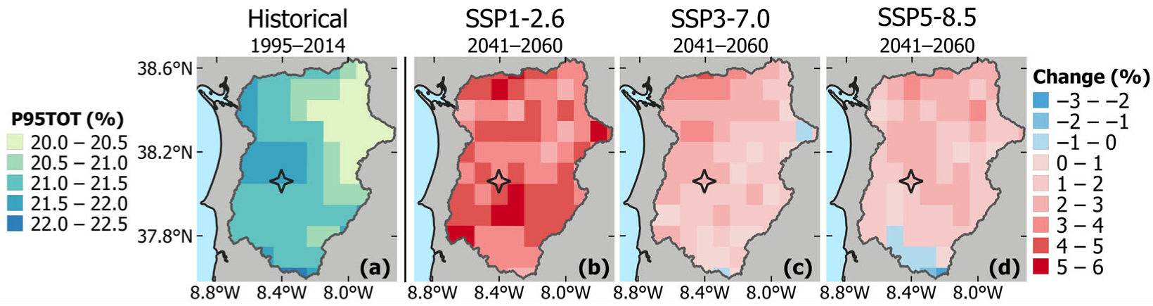
Regarding P95TOT, the historical period data (Figure 5a) reveal a northeast to southwest gradient, with higher values of 21% to 22.5% in the western areas of the basin, and lower values of 20% to 21% in the northeastern areas. As for the changes (Figure 5b–d), no clear spatial pattern emerges. However, the results show that P95TOT is expected to increase between 2% and 6% under SSP1-2.6, and increase between 1% and 4% under SSP3-7.0 and SSP5-8.5. Moreover, small decreases of approximately 1% are projected for the southernmost area under SSP5-8.5.
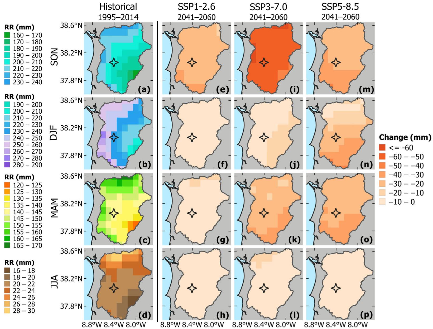
At a seasonal scale, the 1995–2014 total seasonal RR displays higher values during the autumn (SON) and winter (DJF) months, with values declining from winter to spring (MAM), and then from spring to summer (JJA). During SON (Figure 6a), DJF (Figure 6b), and MAM (Figure 6c), there is a southeast to northwest RR gradient, with higher values concentrated in the northern and western areas, and lower values occurring above the southeast area. In JJA (Figure 6d), the gradient is oriented from south to north, yet lower values are also found in the southeast. SON RR varies between 160 and 240 mm, and DJF RR varies between 190 and 290 mm. As for MAM, RR ranges from 120 to 170 mm. JJA present the lower RR values, which vary between 16 and 30 mm.
Regarding the 2041–2060 seasonal RR changes, decreases of up to −60 mm in seasonal RR are expected under all seasons and SSP scenarios. During SON, the SSP1-2.6 scenario (Figure 6e) projects changes between −20 mm and −30 mm in most of the basin, and changes between −30 mm and −40 mm along the basin’s southern parts. In the SSP3-7.0 scenario (Figure 6i), the RR changes range from approximately −50 mm in the southeast areas to below −60 mm in smaller areas along the northern and western borders. The SSP5-8.5 scenario (Figure 6m) presents lower changes than in SSP3-7.0, with −30 to −40 mm changes above south and southwest areas, and −20 to −30 mm changes above north and central areas. In DJF, SSP1-2.6 simulations (Figure 6f) project a uniform RR decrease of 0 to −10 mm throughout the entire basin. Meanwhile, SSP3-7.0 DJF simulations (Figure 6j) indicate that RR could decrease from 0 to −10 mm in the western and northern areas, and from −10 to −20 mm in the eastern areas. SSP5-8.5 changes (Figure 6n) show a more pronounced spatial gradient, pointing towards higher RR decreases of approximately −20 to −40 mm over the southern half of the basin, and lower decreases of 0 to −20 mm over the northern half. Concerning MAM, RR is expected to decrease from 0 to −10 mm in most of the basin under SSP1-2.6 (Figure 6g), while SSP3-7.0 (Figure 6k) and SSP5-8.5 (Figure 6o) present higher RR changes of −30 to −40 mm in the southern areas, and −20 to −30 mm in the northern areas. In the JJA season, projections show a change of 0 to −10 mm for most of the basin under the three SSP scenarios (Figure 6h,l,p).

3.3. Future Changes in Flow Rate and Riverine Water Availability

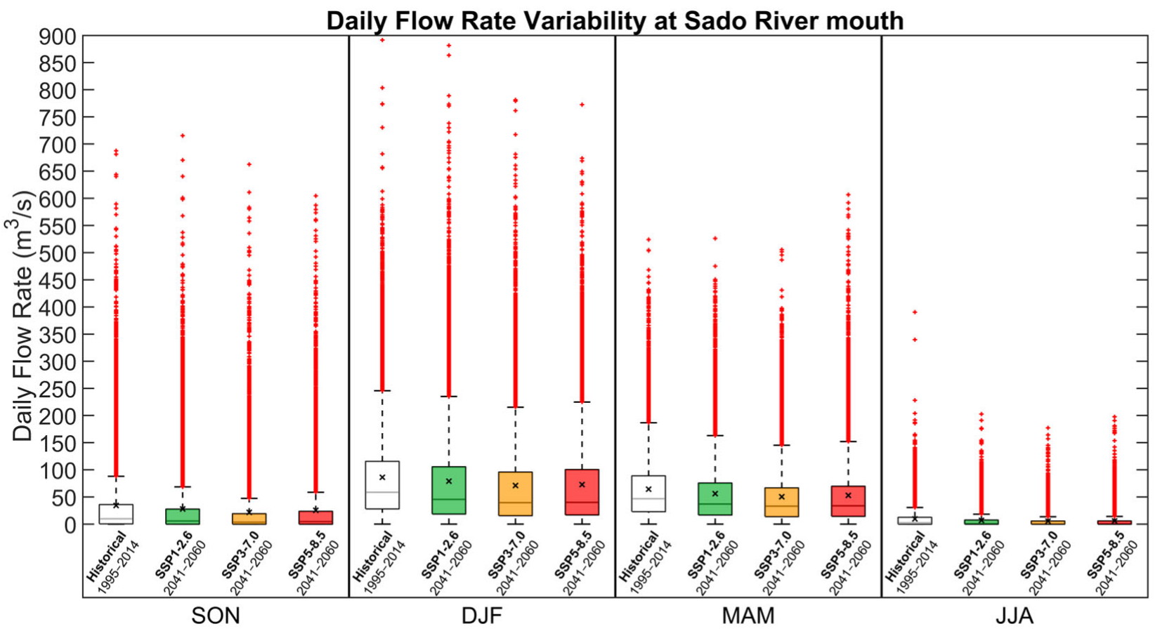
The analysis of HSPF simulation results firstly focused on the daily FR variability at the Sado River mouth (Figure 7).
The statistical analysis considered a data pool of all 20-year daily time series from the nine GCMs. As can be seen in Figure 7, the historical FR regime of the Sado River consists of higher values during DJF, with a non-outlier range of approximately 0–250 m3/s at the river mouth; and lower FR values during JJA, with a non-outlier range of around 0–30 m3/s at the river mouth. During 2041–2060, decreases are projected for the range, mean and median throughout all seasons and scenarios, but mostly under SSP3-7.0, where the relative changes are higher. In addition to the FR variability, the variability of RR and TG at the MG station was also analysed. Regarding RR and TG, it should be mentioned that the non-outlier TG range (Figure S9) is expected to increase during the transition seasons (i.e., SON and MAM) under the three SSP scenarios, and that the non-outlier RR range (Figure S10) is expected to increase during DJF under SSP1-2.6 and SSP3-7.0.
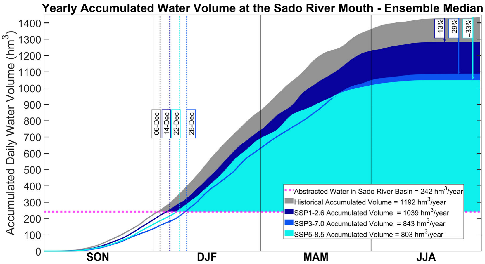
The impacts of the projected FR decrease on the Sado riverine water reserves were assessed by comparing the yearly accumulated riverine water volume with the yearly abstracted surface water volume from the SRB, as presented in Figure 8.
The yearly abstracted surface water volume presented in the Sado RBMP (see Section 1) was used as a reference [31]. By calculating the GCM-ensemble and 20-year median of the yearly accumulated water volume at the river mouth during the hydrological year, it was estimated that a total riverine water volume of 1039 hm3, 843 hm3, and 803 hm3 can be accumulated in the SRB each year under the SSP1-2.6, SSP3-7.0, and SSP5-8.5 scenarios, respectively. Without water abstractions in the basin, these values already represent a decrease of 13%, 29%, and 33%, respectively, in comparison to the historical period, when the yearly accumulated riverine water volume reached 1192 hm3. Nevertheless, the Sado River and its tributaries will still be able to provide at least three times the current surface water needs of the Sado region under SSP3-7.0 and SSP5-8.5. Furthermore, the fulfilment of the region’s yearly surface water needs appears to be achieved later, with the delay reaching as high as 22 days under SSP3-7.0.
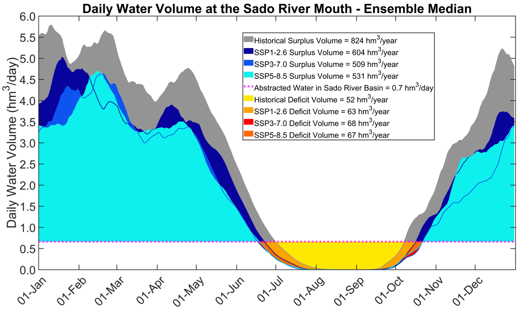
To better understand how riverine water accumulation in the SRB occurs throughout the year, and to identify the seasons with riverine water surplus and deficit, a similar analysis was made using daily water volume data at the Sado River mouth, as presented in Figure 9. Since daily abstracted surface water volume is not available for the SRB, a mean daily abstracted surface water volume of 0.7 hm3/day was considered as the threshold for riverine water surplus and deficit calculations, based on the yearly abstracted surface water volume of 242 hm3/year. The results show that riverine water surplus mainly occurs during DJF and MAM, and that JJA and SON have a deficit. Furthermore, it can also be seen that, from August to mid-September, the daily water volume at the Sado River mouth is null. This suggests that the Sado River and its tributaries might have dried during the simulated reference period, and consequently, no water flow is reaching the Sado River mouth. The highest riverine water surplus volumes are found during DJF and reach up to 5.6 hm3/day under the historical period. Under the SSP scenarios, surplus volumes are expected to experience a large decrease throughout the entire year, which is also visible in Figure 8. The largest reductions in surplus volume are projected under SSP3-7.0, during DJF and MAM. In total, SSP3-7.0 surplus volume is projected to amount to 509 hm3/year, which corresponds to a 38% drop relative to a historical surplus volume of 824 hm3/year. As for JJA and SON, riverine water deficit changes could reach up to 68 hm3/year under SSP3-7.0. This represents an increase of 31% relative to the historical period. Moreover, results also reveal a gradual duration increase in the riverine water deficit period, as well as in the late summer and early autumn river dryness period.

4. Discussion and Conclusions

In this research, future climate projections from a 9-GCM CMIP6 ensemble were used as input to HSPF model simulations of the Sado River Basin (SRB, southwest Portugal). The goal was to simulate possible future flow rates (FRs) and accumulated water volume changes in the Sado River channels between a 2041–2060 near-future period and a 1995–2014 reference period. The future climate data, corresponding to the SSP1-2.6, SSP3-7.0, and SSP5-8.5 socioeconomic scenarios and previously downscaled and bias-adjusted by ISIMIP to a 50 km spatial resolution, were further downscaled to 1 km of spatial resolution using the CHELSA approach, and then bias-adjusted to the SRB’s climate conditions using the ERA5-Iberia 10 km resolution observational dataset. By adjusting and highly increasing the spatial resolution of state-of-the-art global climate ensemble projections over southwest Portugal, this study has not only created an innovative dataset but has also become the first to use downscaled and bias-adjusted CMIP6 ensemble projections as input to hydrological simulations of the SRB. Due to a lack of data regarding the SRB’s reservoir discharges and accumulated volumes, reservoirs were excluded from the model, and thus, future climate impacts in the basin’s surface waters could only be assessed for the riverine waters. The variability of the daily precipitation and mean temperature was also calculated for the historical and future periods, under each of the SSP scenarios. This was done to assess the relations between the future FR changes and the future precipitation/temperature changes.
The projected future FR data reveal that future climate changes could lead to a reduction in the Sado River FR, especially during the autumn (SON), winter (DJF), and spring (MAM) months, when decreases in the mean and median FR are more perceptible. A reduction in the FR range is projected by the HSPF model, which is greater under the SSP3-7.0 scenario. These changes in FR could lead to reductions of 13% (under SSP1-2.6) to 33% (under SSP5-8.5) in the Sado yearly accumulated riverine water volume, and a 22-day delay in the fulfilment of the yearly surface water needs in the Sado region, under SSP3-7.0. Moreover, the accumulation of surplus riverine water volumes, which mostly occurs during DJF and MAM, is expected to decrease under all SSP scenarios and throughout the entire year, with the biggest decrease, of 38%, occurring under the SSP3-7.0 scenario. In the JJA and SON seasons, when Sado surface water needs cannot be fulfilled by the seasons’ FR alone, the riverine water deficit may increase under the three SSP scenarios and reach a 31% increase under SSP3-7.0. Furthermore, the riverine water deficit period may also become longer under all SSP scenarios.
The possible occurrence of FR reductions in the Sado River is related to a decrease in total daily precipitation (RR) and an increase in temperature throughout the year, under all seasons and scenarios. SON and MAM are the seasons with the highest RR decreases, and also an increase in the mean temperature (TG) range. Additionally, a projected increase of up to 6% in P95PTOT indicates that a slightly higher amount of RR will occur under heavy precipitation events in the SRB. Thus, the projected decreases in seasonal and annual RR, along with the increases in the amount of heavy RR and in the DJF RR range under SSP1-2.6 and SSP3-7.0, indicate that yearly RR could become more concentrated in DJF. Finally, the fact that the highest FR and daily riverine water volume losses are projected to occur under SSP3-7.0 is most probably related to the occurrence of higher RR losses during SON (Figure 6) under this scenario.
Despite the differences in the future climatic period considered, similar conclusions were achieved by other studies for the same region, namely, the projected higher runoff reduction during autumn and spring, and lower runoff reduction during winter [16]. As discussed in Section 1, reductions of 19% to 23% in the “Vale do Gaio” reservoir inflows were previously estimated [15]. The discrepancies between the “Vale do Gaio” changes and the present study changes may be attributed not only to the differences in the selected future period, future socioeconomic scenarios, and models, but also to the location of the target area, since the previous study only assessed the flows at the northern part of the basin. Furthermore, similar conclusions were also found for other Mediterranean basins, as is the case of the projected wintertime precipitation concentration and summertime water deficit increase in the Quinto Basin (northeastern Italy) [70]. Hence, the present study not only validates and reinforces the previously obtained results on the SRB water availability but also shows coherence with projections for other Mediterranean basins. Together with previous studies, our results highlight a near-future intensification of riverine water scarcity in the SRB during the spring/summer crop-growing season, a concentration of precipitation in the winter months, and a decrease in riverine water availability throughout the entire year.
The limitations of this study must also be taken into consideration, not only regarding the exclusion of reservoirs from the modelled SRB, but also the lack of observed FR data for hydrological model calibration, and the possible increase in surface water abstractions in the Sado region during the coming decades. The exclusion of reservoirs reduces water storage capacity in the model and possibly underestimates future surface water availability in the basin, while large missing observed FR data periods compromise model calibration, and consequently, the accuracy of FR projections. Hence, future research regarding the SRB hydrology and accumulated surface water resources may consider reservoir dynamics, if sufficient observational data is available. Additionally, improvements in the APA Sado observational stations network should be made to reduce missing and erroneous data and register water abstractions at a monthly or daily scale.
Even though future riverine water volumes should still be able to satisfy consumer water demand in the region, the combination of these changes reveals that wintertime precipitation could become increasingly more relevant for the fulfilment of agricultural water needs in the Sado region during the next decades. Therefore, the availability of wintertime water during summertime agricultural activities should be ensured by storing and preserving enough water to satisfy summertime demands. To achieve this, measures that reduce water waste should be applied, such as improvements in the water supply infrastructure and the use of physical or chemical methods to reduce reservoir water evaporation. Additionally, the increase in current reservoirs and the construction of additional reservoirs may also be necessary. Some of these measures are defended in the 2025 Portuguese Water Management Strategy (PWMS), which also affirms the importance of water in the preservation and promotion of riverine ecosystems during this season [71]. In addition, research on future Sado crop water needs could also be made to support the development of future water demand scenarios by combining crop models and hydrological models tailored to the agriculture sector, such as SWAT. Together with the new PWMS, the outcomes of this study should encourage the regional decision makers and agriculture stakeholders, such as those from the predominant agrarian value chains, to urgently improve wintertime surface water storage, preservation, and management in the SRB in the upcoming decades.

Supplementary Materials

The following supporting information can be downloaded at: https://www.mdpi.com/article/10.3390/w18040442/s1, Figure S1: ISIMIP3b downscaling and bias adjustment workflow.; Figure S2: Correlation between the observed river flow rate at “Moinho da Gamitinha” hydrometric station and the mean 7-day accumulated precipitation in the Sado River Basin, during the 2002–2003 calibration years (a), and 2018 (b) and 2021 (c) validation years.; Figure S3: Total daily precipitation (mm) variability of the 9 General Circulation Models (GCMs) at “Moinho da Gamitinha”, during each season of the 2041–2060 SSP1-2.6 climate scenario.; Figure S4: Total daily precipitation (mm) variability of the 9 General Circulation Models (GCMs) at “Moinho da Gamitinha”, during each season of the 2041–2060 SSP3-7.0 climate scenario.; Figure S5: Total daily precipitation (mm) variability of the 9 General Circulation Models (GCMs) at “Moinho da Gamitinha”, during each season of the 2041–2060 SSP5-8.5 climate scenario.; Figure S6: Daily mean temperature (°C) variability of the 9 General Circulation Models (GCMs) at “Moinho da Gamitinha”, during each season of the 2041–2060 SSP1-2.6 climate scenario.; Figure S7: Daily mean temperature (°C) variability of the 9 General Circulation Models (GCMs) at “Moinho da Gamitinha”, during each season of the 2041–2060 SSP3-7.0 climate scenario.; Figure S8: Daily mean temperature (°C) variability of the 9 General Circulation Models (GCMs) at “Moinho da Gamitinha”, during each season of the 2041–2060 SSP5-8.5 climate scenario.; Figure S9: Daily mean temperature (°C) variability at “Moinho da Gamitinha” in each season. The white, green, yellow, and red boxes represent the 1995–2014 historical period, and the 2041–2060 SSP1-2.6, SSP3-7.0, and SSP5-8.5 scenarios, respectively. Black crosses represent the mean values.; Figure S10: Total daily precipitation (mm) variability at “Moinho da Gamitinha” in each season. The white, green, yellow, and red boxes represent the 1995–2014 historical period, and the 2041–2060 SSP1-2.6, SSP3-7.0, and SSP5-8.5 scenarios, respectively. Black crosses represent the mean values.; Figure S11: Daily flow rate (m3/s) variability at “Moinho da Gamitinha” in each season. The white, green, yellow, and red boxes represent the 1995–2014 historical period, and the 2041–2060 SSP1-2.6, SSP3-7.0, and SSP5-8.5 scenarios, respectively. Black crosses represent the mean values.

Author Contributions

Conceptualisation, A.R.F., C.M., C.A., H.F. and J.A.S.; methodology, A.R.F., C.M., C.A. and J.A.S.; software, A.M.C., A.R.F., A.F. and C.M.; validation, A.M.C., A.R.F., and A.F.; formal analysis, A.M.C., A.R.F. and A.F.; investigation, A.M.C.; resources, C.M. and J.A.S.; data curation, A.M.C. and A.F.; writing—original draft preparation, A.M.C.; writing—review and editing, A.R.F., A.F., C.M., C.A., H.F. and J.A.S.; visualisation, A.M.C.; supervision, A.R.F., C.A., H.F. and J.A.S.; project administration, A.R.F., H.F. and J.A.S.; funding acquisition, A.M.C. and J.A.S. All authors have read and agreed to the published version of the manuscript.

Funding

This research was supported through national funds by FCT—Portuguese Foundation for Science and Technology, under the projects UID/04033/2025; Centre for the Research and Technology of Agro-Environmental and Biological Sciences and LA/P/0126/2020 (https://doi.org/10.54499/LA/P/0126/2020).

Data Availability Statement

The data presented in this study are available upon request from the corresponding authors due to privacy reasons.

Acknowledgments

André M. Claro would like to thank the Massachusetts Institute of Technology (MIT) and the Portuguese Foundation for Science and Technology (FCT) for their support through the MIT Portugal Partnership 2030 (MPP2030-FCT), grant number PRT/BD/154652/2023 (https://doi.org/10.54499/PRT/BD/154652/2023). We also thank project STrengthS4WineChaiN (NORTE2030-FEDER-01786100) and project ReFOOD4North (NORTE2030-FEDER-02654300), funded by the European Regional Development Fund (ERDF) through the Northern Regional Programme 2021-2027 [NORTE2030] and project LivingSoiLL (GA 101157502) funded by Horizon Europe.

Conflicts of Interest

The authors declare no conflicts of interest. The funders had no role in the design of the study; in the collection, analyses, or interpretation of data; in the writing of the manuscript; or in the decision to publish the results.

References

  1. EEA Water Abstraction by Source and Economic Sector in Europe. Available online: https://www.eea.europa.eu/en/analysis/indicators/water-abstraction-by-source-and?activeAccordion= (accessed on 16 August 2025).
  2. Sims, R.E.H. “Energy-Smart” Food for People and Climate; Food and Agriculture Organization of the United Nations (FAO): Rome, Italy, 2011. [Google Scholar]
  3. Moemken, J.; Pinto, J.G. Recurrence of Drought Events Over Iberia. Part I: Methodology and Application for Present Climate Conditions. Tellus A Dyn. Meteorol. Oceanogr. 2022, 74, 222. [Google Scholar] [CrossRef] [Scilit]
  4. Andrade, C.; Corte-Real, J. Aridity Conditions in the Iberian Peninsula during the XX Century. Int. J. Environ. Sci. 2016, 1, 52–58. [Google Scholar]
  5. Páscoa, P.; Russo, A.; Gouveia, C.M.; Soares, P.M.M.; Cardoso, R.M.; Careto, J.A.M.; Ribeiro, A.F.S. A High-Resolution View of the Recent Drought Trends over the Iberian Peninsula. Weather Clim. Extrem. 2021, 32, 100320. [Google Scholar] [CrossRef] [Scilit]
  6. Andrade, C.; Contente, J.; Santos, J.A. Climate Change Projections of Dry and Wet Events in Iberia Based on the WASP-Index. Climate 2021, 9, 94. [Google Scholar] [CrossRef] [Scilit]
  7. Todeschini, S. Trends in Long Daily Rainfall Series of Lombardia (Northern Italy) Affecting Urban Stormwater Control. Int. J. Climatol. 2012, 32, 900–919. [Google Scholar] [CrossRef] [Scilit]
  8. Pereira, S.C.; Carvalho, D.; Rocha, A. Temperature and Precipitation Extremes over the Iberian Peninsula under Climate Change Scenarios: A Review. Climate 2021, 9, 139. [Google Scholar] [CrossRef] [Scilit]
  9. Soares, P.M.M.; Careto, J.A.M.; Russo, A.; Lima, D.C.A. The Future of Iberian Droughts: A Deeper Analysis Based on Multi-Scenario and a Multi-Model Ensemble Approach. Nat. Hazards 2023, 117, 2001–2028. [Google Scholar] [CrossRef] [Scilit]
  10. García-Valdecasas Ojeda, M.; Gámiz-Fortis, S.R.; Romero-Jiménez, E.; Rosa-Cánovas, J.J.; Yeste, P.; Castro-Díez, Y.; Esteban-Parra, M.J. Projected Changes in the Iberian Peninsula Drought Characteristics. Sci. Total Environ. 2021, 757, 143702. [Google Scholar] [CrossRef] [Scilit]
  11. Sondermann, M.N.; de Oliveira, R.P. Climate Adaptation Needs to Reduce Water Scarcity Vulnerability in the Tagus River Basin. Water 2022, 14, 2527. [Google Scholar] [CrossRef] [Scilit]
  12. CEDEX. Evaluación Del Impacto Del Cambio Climático En Los Recursos Hídricos Y Sequías En España; CEDEX: Madrid, Spain, 2017. [Google Scholar]
  13. Pellicer-Martínez, F.; Martínez-Paz, J.M. Climate Change Effects on the Hydrology of the Headwaters of the Tagus River: Implications for the Management of the Tagus–Segura Transfer. Hydrol. Earth Syst. Sci. 2018, 22, 6473–6491. [Google Scholar] [CrossRef] [Scilit]
  14. Ministério do Ambiente e do Ordenamento do Território. Decreto Regulamentar n.o 6/2002; MAOT: Lisboa, Portugal, 2002; pp. 1090–1138. [Google Scholar]
  15. Nunes, J.P.; Jacinto, R.; Keizer, J.J. Combined Impacts of Climate and Socio-Economic Scenarios on Irrigation Water Availability for a Dry Mediterranean Reservoir. Sci. Total Environ. 2017, 584–585, 219–233. [Google Scholar] [CrossRef] [Scilit] [PubMed]
  16. Mourato, S.; Moreira, M.; Corte-Real, J. Water Resources Impact Assessment Under Climate Change Scenarios in Mediterranean Watersheds. Water Resour. Manag. 2015, 29, 2377–2391. [Google Scholar] [CrossRef] [Scilit]
  17. APA. Plano de Gestão de Região Hidrográfica—3o Ciclo (2022–2027)—Sado e Mira (RH6)–Resumo Não Técnico; APA: Lisboa, Portugal, 2023. [Google Scholar]
  18. APA. Avaliação Preliminar de Risco de Inundações RH6—Sado e Mira; APA: Lisboa, Portugal, 2019. [Google Scholar]
  19. APSS. Áreas Logísticas. Available online: https://www.portodesetubal.pt/setubal/pagina/45/areas-logisticas (accessed on 31 December 2025).
  20. APP. Porto de Setúbal. Available online: https://www.portosdeportugal.pt/app/portos/setubal.php (accessed on 31 December 2025).
  21. Nascimento, Â.; Biguino, B.; Borges, C.; Cereja, R.; Cruz, J.P.C.; Sousa, F.; Dias, J.; Brotas, V.; Palma, C.; Brito, A.C. Tidal Variability of Water Quality Parameters in a Mesotidal Estuary (Sado Estuary, Portugal). Sci. Rep. 2021, 11, 23112. [Google Scholar] [CrossRef] [Scilit]
  22. SNIAmb. Atlas Da Água—Rede Hidrográfica Total. Available online: https://sniambgeoviewer.apambiente.pt/GeoDocs/shpzips/AtAgua_Agsup_zhidnetord5km2_PC.zip (accessed on 11 August 2025).
  23. European Environmental Agency EU-DEM (Raster)—Version 1.1, April 2016. Available online: https://sdi.eea.europa.eu/catalogue/srv/api/records/3473589f-0854-4601-919e-2e7dd172ff50 (accessed on 23 October 2023).
  24. Köppen, W. Das Geographische System Der Klimate. In Handbuch der Klimatologie; Köppen, W., Geiger, R., Eds.; Borntraeger: Berlin, Germany, 1936; Volume 1. [Google Scholar]
  25. Geiger, R. Klassifikation Der Klimate Nach W. Köppen. In Landolt-Börnstein—Zahlenwerte und Funktionen aus Physik, Chemie, Astronomie, Geophysik und Technik; Springer: Berlin, Germany, 1954; Volume 3, pp. 603–607. [Google Scholar]
  26. Beck, H.E.; Zimmermann, N.E.; McVicar, T.R.; Vergopolan, N.; Berg, A.; Wood, E.F. Present and Future Köppen-Geiger Climate Classification Maps at 1-Km Resolution. Sci. Data 2018, 5, 180214. [Google Scholar] [CrossRef] [Scilit]
  27. Claro, A.M.; Fonseca, A.; Fraga, H.; Santos, J.A. Susceptibility of Iberia to Extreme Precipitation and Aridity: A New High-Resolution Analysis over an Extended Historical Period. Water 2023, 15, 3840. [Google Scholar] [CrossRef] [Scilit]
  28. IPMA. Normais Climatológicas 1991–2020. Available online: https://www.ipma.pt/pt/oclima/normais.clima/1991-2020/normalclimate9120.jsp (accessed on 11 August 2025).
  29. SNIRH. Dados de Base—Moinho Da Gamitinha. Available online: https://snirh.apambiente.pt/snirh/_dadosbase/site/simplex.php?OBJINFO=DADOS&FILTRA_BACIA=38&FILTRA_COVER=920123705&FILTRA_SITE=1627758798 (accessed on 11 August 2025).
  30. Vale, C.; Cortesão, C.; Castro, O.; Ferreira, A.M. Suspended-Sediment Response to Pulses in River Flow and Semidiurnal and Fortnightly Tidal Variations in a Mesotidal Estuary. Mar. Chem. 1993, 43, 21–31. [Google Scholar] [CrossRef] [Scilit]
  31. APA. Plano de Gestão de Região Hidrográfica—3o Ciclo (2022–2027)—Sado e Mira (RH6)—Parte 2: Caracterização e Diagnóstico; APA: Lisboa, Portugal, 2023; Volume A. [Google Scholar]
  32. Eyring, V.; Bony, S.; Meehl, G.A.; Senior, C.A.; Stevens, B.; Stouffer, R.J.; Taylor, K.E. Overview of the Coupled Model Intercomparison Project Phase 6 (CMIP6) Experimental Design and Organization. Geosci. Model Dev. 2016, 9, 1937–1958. [Google Scholar] [CrossRef] [Scilit]
  33. O’Neill, B.C.; Tebaldi, C.; van Vuuren, D.P.; Eyring, V.; Friedlingstein, P.; Hurtt, G.; Knutti, R.; Kriegler, E.; Lamarque, J.-F.; Lowe, J.; et al. The Scenario Model Intercomparison Project (ScenarioMIP) for CMIP6. Geosci. Model Dev. 2016, 9, 3461–3482. [Google Scholar] [CrossRef] [Scilit]
  34. Swart, N.C.; Cole, J.N.S.; Kharin, V.V.; Lazare, M.; Scinocca, J.F.; Gillett, N.P.; Anstey, J.; Arora, V.; Christian, J.R.; Hanna, S.; et al. The Canadian Earth System Model Version 5 (CanESM5.0.3). Geosci. Model Dev. 2019, 12, 4823–4873. [Google Scholar] [CrossRef] [Scilit]
  35. Voldoire, A.; Saint-Martin, D.; Sénési, S.; Decharme, B.; Alias, A.; Chevallier, M.; Colin, J.; Guérémy, J.-F.; Michou, M.; Moine, M.-P.; et al. Evaluation of CMIP6 DECK Experiments With CNRM-CM6-1. J. Adv. Model. Earth Syst. 2019, 11, 2177–2213. [Google Scholar] [CrossRef] [Scilit]
  36. Séférian, R.; Nabat, P.; Michou, M.; Saint-Martin, D.; Voldoire, A.; Colin, J.; Decharme, B.; Delire, C.; Berthet, S.; Chevallier, M.; et al. Evaluation of CNRM Earth System Model, CNRM-ESM2-1: Role of Earth System Processes in Present-Day and Future Climate. J. Adv. Model. Earth Syst. 2019, 11, 4182–4227. [Google Scholar] [CrossRef] [Scilit]
  37. Döscher, R.; Acosta, M.; Alessandri, A.; Anthoni, P.; Arsouze, T.; Bergman, T.; Bernardello, R.; Boussetta, S.; Caron, L.P.; Carver, G.; et al. The EC-Earth3 Earth System Model for the Coupled Model Intercomparison Project 6. Geosci. Model Dev. 2022, 15, 2973–3020. [Google Scholar] [CrossRef] [Scilit]
  38. Boucher, O.; Servonnat, J.; Albright, A.L.; Aumont, O.; Balkanski, Y.; Bastrikov, V.; Bekki, S.; Bonnet, R.; Bony, S.; Bopp, L.; et al. Presentation and Evaluation of the IPSL-CM6A-LR Climate Model. J. Adv. Model. Earth Syst. 2020, 12, e2019MS002010. [Google Scholar] [CrossRef] [Scilit]
  39. MIROC6 AGCM Document Writing Team. Description of MIROC6 AGCM; MIROC6 AGCM Document Writing Team: Tokyo, Japan, 2021. [Google Scholar]
  40. Müller, W.A.; Jungclaus, J.H.; Mauritsen, T.; Baehr, J.; Bittner, M.; Budich, R.; Bunzel, F.; Esch, M.; Ghosh, R.; Haak, H.; et al. A Higher-Resolution Version of the Max Planck Institute Earth System Model (MPI-ESM1.2-HR). J. Adv. Model. Earth Syst. 2018, 10, 1383–1413. [Google Scholar] [CrossRef] [Scilit]
  41. Yukimoto, S.; Kawai, H.; Koshiro, T.; Oshima, N.; Yoshida, K.; Urakawa, S.; Tsujino, H.; Deushi, M.; Tanaka, T.; Hosaka, M.; et al. The Meteorological Research Institute Earth System Model Version 2.0, MRI-ESM2.0: Description and Basic Evaluation of the Physical Component. J. Meteorol. Soc. Jpn. Ser. II 2019, 97, 931–965. [Google Scholar] [CrossRef] [Scilit]
  42. Sellar, A.A.; Jones, C.G.; Mulcahy, J.P.; Tang, Y.; Yool, A.; Wiltshire, A.; O’Connor, F.M.; Stringer, M.; Hill, R.; Palmieri, J.; et al. UKESM1: Description and Evaluation of the U.K. Earth System Model. J. Adv. Model. Earth Syst. 2019, 11, 4513–4558. [Google Scholar] [CrossRef] [Scilit]
  43. IPCC Summary for Policymakers. Climate Change 2023: Synthesis Report. Contribution of Working Groups I, II and III to the Sixth Assessment Report of the Intergovernmental Panel on Climate Change; Lee, H., Romero, J., Eds.; IPCC: Geneva, Switzerland, 2023; pp. 1–34. [Google Scholar]
  44. Warszawski, L.; Frieler, K.; Huber, V.; Piontek, F.; Serdeczny, O.; Schewe, J. The Inter-Sectoral Impact Model Intercomparison Project (ISI–MIP): Project Framework. Proc. Natl. Acad. Sci. USA 2014, 111, 3228–3232. [Google Scholar] [CrossRef] [Scilit] [PubMed]
  45. ISIMIP. ISIMIP3 Protocol. Available online: https://www.isimip.org/protocol/3/ (accessed on 11 August 2025).
  46. Lange, S.; Büchner, M. ISIMIP3b Bias-Adjusted Atmospheric Climate Input Data, Version: 1.1; ISIMIP Repository: Potsdam, Germany, 2021. [Google Scholar] [CrossRef] [Scilit]
  47. Lange, S.; Menz, C.; Gleixner, S.; Cucchi, M.; Weedon, G.P.; Amici, A.; Bellouin, N.; Schmied, H.M.; Hersbach, H.; Buontempo, C.; et al. WFDE5 over Land Merged with ERA5 over the Ocean (W5E5 v2.0), Version 2.0; ISIMIP Repository: Potsdam, Germany, 2021. [Google Scholar]
  48. Karger, D.N.; Conrad, O.; Böhner, J.; Kawohl, T.; Kreft, H.; Soria-Auza, R.W.; Zimmermann, N.E.; Linder, H.P.; Kessler, M. Climatologies at High Resolution for the Earth’s Land Surface Areas. Sci. Data 2017, 4, 170122. [Google Scholar] [CrossRef] [Scilit]
  49. Teutschbein, C.; Seibert, J. Bias Correction of Regional Climate Model Simulations for Hydrological Climate-Change Impact Studies: Review and Evaluation of Different Methods. J. Hydrol. 2012, 456–457, 12–29. [Google Scholar] [CrossRef] [Scilit]
  50. Piani, C.; Weedon, G.P.; Best, M.; Gomes, S.M.; Viterbo, P.; Hagemann, S.; Haerter, J.O. Statistical Bias Correction of Global Simulated Daily Precipitation and Temperature for the Application of Hydrological Models. J. Hydrol. 2010, 395, 199–215. [Google Scholar] [CrossRef] [Scilit]
  51. Herrera, S.; Cardoso, R.M.; Soares, P.M.; Espírito-Santo, F.; Viterbo, P.; Gutiérrez, J.M. Iberia01: A New Gridded Dataset of Daily Precipitation and Temperatures over Iberia. Earth Syst. Sci. Data 2019, 11, 1947–1956. [Google Scholar] [CrossRef] [Scilit]
  52. Muñoz Sabater, J. ERA5-Land Hourly Data from 1950 to Present. Available online: https://doi.org/10.24381/cds.e2161bac (accessed on 4 February 2026).
  53. Miao, C.; Su, L.; Sun, Q.; Duan, Q. A Nonstationary Bias-Correction Technique to Remove Bias in GCM Simulations. J. Geophys. Res. Atmos. 2016, 121, 5718–5735. [Google Scholar] [CrossRef] [Scilit]
  54. Wang, L.; Chen, W. Equiratio Cumulative Distribution Function Matching as an Improvement to the Equidistant Approach in Bias Correction of Precipitation. Atmos. Sci. Lett. 2014, 15, 1–6. [Google Scholar] [CrossRef] [Scilit]
  55. Li, H.; Sheffield, J.; Wood, E.F. Bias Correction of Monthly Precipitation and Temperature Fields from Intergovernmental Panel on Climate Change AR4 Models Using Equidistant Quantile Matching. J. Geophys. Res. 2010, 115, D10101. [Google Scholar] [CrossRef] [Scilit]
  56. Duda, P.B.; Hummel, P.R.; Donigian, A.S., Jr.; Imhoff, J.C. BASINS/HSPF: Model Use, Calibration, and Validation. Trans. ASABE 2012, 55, 1523–1547. [Google Scholar] [CrossRef] [Scilit]
  57. Donigian, A.S.; Davis, H.H. User’s Manual for Agricultural Runoff Management (ARM) Model; Environmental Research Laboratory, Office of Research and Development: Washington, DC, USA, 1978. [Google Scholar]
  58. Donigian, A.S.; Crawford, N.H. Modeling Nonpoint Pollution from the Land Surface; U.S. Environmental Protection Agency, Office of Research and Development, Environmental Research Laboratory: Athens, GA, USA, 1976. [Google Scholar]
  59. Donigian, A.S.; Bicknell, B.R.; Imhoff, J.C. Hydrological Simulation Program—Fortran (HSPF). In Computer Models of Watershed Hydrology; Water Resource Publications: Littleton, CO, USA, 1995; Volume 12, pp. 395–442. ISBN 978-0-918334-91-6. [Google Scholar]
  60. Marcé, R.; Ruiz, C.E.; Armengol, J. Using Spatially Distributed Parameters and Multi-response Objective Functions to Solve Parameterization of Complex Applications of Semi-distributed Hydrological Models. Water Resour. Res. 2008, 44, 2–3. [Google Scholar] [CrossRef] [Scilit]
  61. Johnson, M.S.; Coon, W.F.; Mehta, V.K.; Steenhuis, T.S.; Brooks, E.S.; Boll, J. Application of Two Hydrologic Models with Different Runoff Mechanisms to a Hillslope Dominated Watershed in the Northeastern US: A Comparison of HSPF and SMR. J. Hydrol. 2003, 284, 57–76. [Google Scholar] [CrossRef] [Scilit]
  62. Duda, P.B.; Kittle, J.L., Jr.; Donigian, A.S., Jr.; Kinerson, R.S. Better Assessment Science Integrating Point and Nonpoint Sources (BASINS). In Watershed Models; Singh, V.P., Frevert, D.K., Eds.; CRC Press: Boca Raton, FL, USA, 2010; pp. 273–290. ISBN 9780429122446. [Google Scholar]
  63. do Território, D.-G. Especificações Técnicas Da Carta de Uso e Ocupação Do Solo (COS) de Portugal Continental Para 2018; Direção-Geral do Território: Lisboa, Portugal, 2019. [Google Scholar]
  64. FAO. Harmonized World Soil Database Version 2.0; Food and Agriculture Organization (FAO): Rome, Italy; International Institute for Applied Systems Analysis (IIASA): Laxenburg, Austria, 2023; ISBN 978-92-5-137499-3. [Google Scholar]
  65. Hummel, P.; Kittle, J., Jr.; Gray, M. WDMUtil, A Tool for Managing Watershed Modeling Time-Series Data—User’s Manual; United States Environmental Protection Agency: Washington, DC, USA, 2001. [Google Scholar]
  66. Nash, J.E.; Sutcliffe, J.V. River Flow Forecasting through Conceptual Models Part I—A Discussion of Principles. J. Hydrol. 1970, 10, 282–290. [Google Scholar] [CrossRef] [Scilit]
  67. Draper, N.R.; Smith, H. Applied Regression Analysis, 3rd ed.; McGraw-Hill Inc.: New York, NY, USA, 1998; ISBN 0-471-17082-8. [Google Scholar]
  68. Yapo, P.O.; Gupta, H.V.; Sorooshian, S. Automatic Calibration of Conceptual Rainfall-Runoff Models: Sensitivity to Calibration Data. J. Hydrol. 1996, 181, 23–48. [Google Scholar] [CrossRef] [Scilit]
  69. The MathWorks Inc. MATLAB, Version: 9.14.0 (R2023a); The MathWorks Inc.: Natick, MA, USA, 2023.
  70. Mollema, P.; Antonellini, M.; Gabbianelli, G.; Laghi, M.; Marconi, V.; Minchio, A. Climate and Water Budget Change of a Mediterranean Coastal Watershed, Ravenna, Italy. Environ. Earth Sci. 2012, 65, 257–276. [Google Scholar] [CrossRef] [Scilit]
  71. XXIV Governo da República Portuguesa Água Que Une. In Estratégia Nacional Para a Gestão Da Água; XXIV Governo da República Portuguesa Água Que Une: Lisboa, Portugal, 2025.
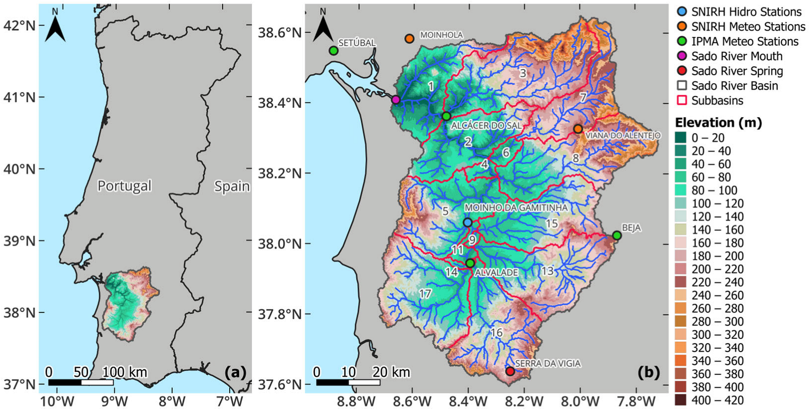
Figure 1. Location of the Sado River Basin in Portugal (a), and location of the basin’s water channels ((b), blue lines), subbasins (numbers and red lines), Sado River spring ((b), red dot), Sado River mouth ((b), purple dot), IPMA meteorological stations ((b), green dots), SNIRH meteorological stations ((b), orange dots), and SNIRH hydrometric station (blue dot). The basin’s hypsometric chart is represented in the background.
Water 18 00442 g001
Figure 2. Comparison between the monthly mean observed flow rate (black) and simulated flow rate (blue, red) during the 2002–2003 calibration years ((a), blue), and 2018 (b) and 2021 (c) validation (red) years. The grey bars represent the monthly total observed precipitation.
Water 18 00442 g002
Figure 3. General Circulation Model ensemble median of the 20-year mean daily maximum (TX, (a,d,g,j)), mean (TG, (b,e,h,k)), and minimum (TN, (c,f,i,l)) temperatures (°C) during the 1995–2014 historical period (1st column), and the respective 2041–2060 ensemble median changes under the SSP1-2.6 (2nd column), SSP3-7.0 (3rd column), and SSP5-8.5 (4th column) scenarios. The black star indicates the location of the MG hydrometric station.
Water 18 00442 g003
Figure 4. General Circulation Model ensemble median of the 20-year mean total annual precipitation (RR, mm/year) during the 1995–2014 historical period (a), as well as the respective 2041–2060 ensemble median changes under the SSP1-2.6 (b), SSP3-7.0 (c), and SSP5-8.5 (d) scenarios. The black star indicates the location of the MG hydrometric station.
Water 18 00442 g004
Figure 5. General Circulation Model ensemble median of the percentage of 20-year total precipitation above the 1995–2014 total precipitation’s 95th percentile (P95TOT, %) during the 1995–2014 historical period (a), as well as the respective 2041–2060 ensemble median changes under the SSP1-2.6 (b), SSP3-7.0 (c), and SSP5-8.5 (d) scenarios. The black star indicates the location of the MG hydrometric station.
Water 18 00442 g005
Figure 6. GCM ensemble median of the 20-year mean total autumn (SON, (a,e,i,m)), winter (DJF, (b,f,j,n)), spring (MAM, (c,g,k,o)) and summer (JJA, (d,h,l,p)) precipitation (RR, mm/season) during the 1995–2014 historical period (1st column), and the respective 2041–2060 ensemble median changes under the SSP1-2.6 (2nd column), SSP3-7.0 (3rd column), and SSP5-8.5 (4th column) scenarios. The black star indicates the location of the MG hydrometric station.
Water 18 00442 g006
Figure 7. Daily flow rate (m3/s) variability at the Sado River mouth, in each season. The white, green, yellow, and red boxes represent the 1995–2014 historical and 2041–2060 SSP1-2.6, SSP3-7.0, and SSP5-8.5 scenarios, respectively. Black crosses represent the mean values.
Water 18 00442 g007
Figure 8. Ensemble and time-median yearly accumulated riverine water volume (hm3) simulated at the Sado River mouth during the 1995–2014 historical period (grey line), and the 2041–2060 SSP1-2.6 (dark blue line), SSP3-7.0 (cyan line), and SSP5-8.5 (medium blue line) scenarios. The magenta dashed line represents the yearly surface water abstractions in the Sado River Basin, while the grey, dark blue, cyan, and medium blue shaded areas represent each scenario’s yearly accumulated surplus volume. Grey, dark blue, cyan, and medium blue dashed lines indicate the date when total yearly surface water needs are fulfilled. The blue arrows indicate the relative changes in future accumulated volumes.
Water 18 00442 g008
Figure 9. Ensemble and time-median daily riverine water volume (hm3/day) simulated at the Sado River mouth during one year under the 1995–2014 historical period (grey line), and under the 2041–2060 SSP1-2.6 (dark blue line), SSP3-7.0 (cyan line), and SSP5-8.5 (medium blue line) scenarios. The magenta dashed line represents the daily water abstractions in the Sado River Basin, while the grey, dark blue, cyan and medium blue shaded areas represent each scenario’s riverine surplus volume. The yellow, light orange, red, and dark orange shaded areas represent the riverine deficit volume during the summer and autumn months, under the historical, SSP1-2.6, SSP3-7.0, and SSP5-8.5 scenarios, respectively.
Water 18 00442 g009
Table 1. List of the ISIMIP3b General Circulation Models (GCMs) used in this research.
GCMInstitutionCitation
CanESM5Canadian Centre for Climate Modelling and Analysis (CCCma), Canada[34]
CNRM-CM6-1Centre National de Recherches Météorologiques (CNRM), France[35]
CNRM-ESM2-1[36]
EC-Earth3EC-Earth-Consortium (12 European countries)[37]
IPSL-CM6A-LRInstitut Pierre Simon Laplace (IPSL), France[38]
MIROC6Japan Agency for Marine-Earth Science and Technology (JAMSTEC), Japan[39]
MPI-ESM1-2-HRMax Planck Institute for Meteorology (MPI-M), Germany[40]
MRI-ESM2-0Meteorological Research Institute (MRI), Japan[41]
UKESM1-0-LLMet Office, United Kingdom[42]
Table 2. List of the selected values (VAL) for the HSPF model parameters (PAR) and imperviousness percentages (IMP) that were adjusted during model calibration.
Yearly PARVALMonthly
PAR
VALMonthly
PAR
VALLand Use GroupIMP
LZSN (in)13INT_JAN0.05LZE_JAN0.2Agriculture10%
UZSN (in)8INT_FEB0.01LZE_FEB0.2Wetlands70%
LSUR (ft)200INT_MAR0.02LZE_MAR0.3Pasture10%
SLSUR0.131INT_APR0.0001LZE_APR0.3Urban50%
NSUR1INT_MAY0.003LZE_MAY0.4Forestry20%
INTFW5INT_JUN0.003LZE_JUN0.4Shrublands20%
CEPSC (in)0.005INT_JUL0.003LZE_JUL0.4
INFILT (in/hr)15INT_AUG0.003LZE_AUG0.4
AGWRC (1/day)0.96INT_SEP0.0001LZE_SEP0.4
INT_OCT0.005LZE_OCT0.3
INT_NOV0.005LZE_NOV0.2
INT_DEC0.005LZE_DEC0.2
Table 3. Model calibration performance and annual metrics for the monthly flow rates (FR) and annual precipitation (RR).
Monthly FRAnnual RR (mm/year)Annual Mean FR (m3/s)
NSER2PBIASObservedObservedSimulated
2002–20030.780.80−4%5975.355.11
20180.780.799%3313.103.37
20210.810.90−6%4873.593.37
Disclaimer/Publisher’s Note: The statements, opinions and data contained in all publications are solely those of the individual author(s) and contributor(s) and not of MDPI and/or the editor(s). MDPI and/or the editor(s) disclaim responsibility for any injury to people or property resulting from any ideas, methods, instructions or products referred to in the content.