Article

An In-Depth Statistical Analysis of the Pearson Type III Distribution Behavior in Modeling Extreme and Rare Events

by
Cristian-Gabriel Anghel
* and
Dan Ianculescu
*
Faculty of Hydrotechnics, Technical University of Civil Engineering Bucharest, Lacul Tei, nr.122-124, 020396 Bucharest, Romania
*
Authors to whom correspondence should be addressed.
Water 2025, 17(10), 1539; https://doi.org/10.3390/w17101539
Submission received: 28 March 2025 / Revised: 17 May 2025 / Accepted: 17 May 2025 / Published: 20 May 2025
(This article belongs to the Special Issue Urban Flood Frequency Analysis and Risk Assessment)

Abstract

:
Statistical distributions play a crucial role in water resources management and civil engineering, particularly for analyzing data variability and predicting rare events with extremely long return periods (e.g., T = 1000 years, T = 10,000 years). Among these, the Pearson III (PE3) distribution is widely used in hydrology and flood frequency analysis (FFA). This study aims to provide a comprehensive guide to the practical application of the PE3 distribution in FFA. It explores five parameter estimation methods, presenting both exact and newly developed approximate relationships for calculating distribution parameters and frequency factors. The analysis relies on data from four rivers with varying morphometric characteristics and record lengths. The results highlight that the Pearson III distribution, when used with the L-moments method, offers the most reliable quantile estimates, characterized by the smallest biases compared to other methods (e.g., 31% for the Nicolina River and, respectively, 5% for the Siret and Ialomita Rivers) and the highest confidence in predicting rare events. Based on these findings, the L-moments approach is recommended for flood frequency analysis to improve the accuracy of extreme flow forecasts.

1. Introduction

Water management relies heavily on statistical distributions because they offer a framework for comprehending and evaluating the variability of hydrological data. They give managers of water resources information on the annual exceedance probability of various hydrological events, empowering them to plan ahead and make wise decisions that promote the sustainable use of water resources.
The most important contributions of probability distributions in water management are precipitation analysis, river flow management, hydrological risk assessment, reservoir management, water demand estimation, climate change modeling, groundwater management, water quality monitoring, and the hydrological component in establishing bankfull discharge.
In flood frequency analysis (FFA), this allows for calculating values that have a specified probability of occurrence, especially the extreme values considered “impossible floods”, a critical aspect in water resource management and the planning of hydrotechnical projects such as dams and levees. “Impossible floods’’ are “large events, or different types of events, that exceed the expectations based on historical experience. Such impossible events include floods whose probability of occurrence is considered too small to act, but also events that go beyond any imagination” [1].
The Pearson III (PE3) distribution, a variant of the four-parameter gamma distribution and a generalized two-parameter gamma distribution, is widely utilized in the statistical analysis of extreme data, alongside distributions like log-normal (LN3), generalized extreme value (GEV, including Weibull, Gumbel and Fréchet distributions), and log-Pearson III distributions [2,3,4,5,6,7,8]. It has been extensively applied in various studies, including for flood frequency analysis [6,9,10,11,12,13,14,15,16,17], for maximum rainfall frequency analysis [18,19,20,21], and for low flow frequency analysis [5,22,23,24,25,26], employing different parameter estimation methods. In Romania, PE3 has been adopted as the ‘’parent’’ distribution in flood frequency investigations [16,17], using a simplistic approach based on the Foster–Ribkin table.
Since the quantile function lacks a closed-form expression, this manuscript proposes a practical definition using the predefined Excel function Gamma.INV. Depending on the estimation method, the quantile function can integrate the frequency factor, offering a useful approach, especially given that the inverse is defined through the gamma function.
In at-site frequency analysis, parameters are estimated using various methods. In contrast, regional frequency analysis relies on statistical indicators specific to each region. Only two methods use these regional indicators for parameter estimation: the method of ordinary moments and the method of linear moments. Internationally, the method of linear moments is preferred due to its rigor, stability, and robustness, as demonstrated by extensive research. These strengths make it suitable for both at-site and regional analyses.
Unfortunately, Romanian regulations have not yet adopted the consistent use of the L-moments in either context.
Typically, the PE3 distribution is parameterized using the method of ordinary moments (MOM) and the linear moments (L-moments) method, which are among the most commonly used techniques in FFA [2,5,6,11,27,28]. Compared to other methods, the L-moments approach is noted for its greater stability and reduced bias [6,9,29,30,31]. Another method, LH-moments (the higher-order linear moments), first proposed by Wang in 1997 [30], introduces a “separation effect” [31,32], which quickly gained popularity in FFA applications. This method is particularly recommended when using the Annual Maximum Series (AMS), as it minimizes the influence of smaller maximum values in frequency analysis by extending the concept of linear moments. Consequently, it enhances the significance of higher maximum values, which typically represent flood events.
In terms of parameter estimation methods, MOM is commonly preferred for its simplicity and ease of use in estimation formulas. However, a drawback is the need for the correction of higher-order statistical indicators, such as skewness and kurtosis. A solution to correct the skewness coefficient is provided by the method developed by Bobée and Robitaille [2,3,6,28]. In Romania, this issue has been partially addressed by adjusting skewness based on the origin of maximum flows. According to Romanian regulations [13], a skewness coefficient of two is chosen for maximum flows from snow melt, three for mixed origins (snow melt and rain), and four for peak flows exclusively from rainfall. This approach, however, is often misapplied and overly generalized, as it applies strictly to hydrographic basins smaller than 100 km2 and assumes a coefficient of variation of one for maximum flows solely from rainfall.
Estimating parameters using L- and LH-moments requires solving a system of nonlinear equations, which can be challenging. To simplify this process, new and improved approximation relationships are introduced using polynomial, exponential, or rational functions. Hosking and Wallis [9] made a significant contribution by providing equations for estimating the shape parameter, improving the usability and accuracy of the parameter estimation method using L-moments. The LH-moments method has seen significant advancements, as documented by [32,33,34,35,36,37,38,39,40,41], with an extensive analysis covering several important distributions, including Wakeby, Lambda, Pearson V, CHI, inverse CHI, Wilson–Hilferty, pseudo-Weibull, log-normal, and various forms of generalized Pareto (Type I, II, III, and IV), as well as the Fréchet distribution.
Regarding the LSM, the study conducts a comparative analysis to determine the optimal empirical probability fitting the PE3 distribution, aiming to minimize errors at three levels: statistical indicators, parameter estimation, and forecasted values. For the MLE, valid solutions for the parameters of the PE3 distribution are achievable only when the skewness coefficient is less than two. This criterion is highlighted in both the current analysis and observations by other researchers [6,28].
Since uncertainties are inherent in all statistical analyses, this manuscript details methods for calculating confidence intervals for the Pearson III distribution, essential for quantifying these uncertainties. It includes Chow’s approximation (utilized for MOM, L-moments, and LH-moments) and the Kite approximation (specifically for MOM), providing a means to establish confidence intervals at a 95% level. Chow’s method assumes a Gaussian distribution, offering a simplified approach in these calculations.
Typically, quantiles exceeding the probabilities of recorded values exhibit significant uncertainty due to the relatively short length of the observed data. Thus, the manuscript discusses three interconnected levels of uncertainty:
(a)
arising from the limited length of available recorded data;
(b)
associated with parameter estimation;
(c)
concerning uncertainties in predicted quantile values.
These uncertainties, along with various estimation techniques and data lengths, are explored in the context of the Pearson III distribution.
In general, the direct forecasting of quantiles involves certain essential steps, the most important being:
-
choosing the best model (the best statistical distribution according to different parameter estimation methods and certain hydrological and statistical characteristics, a holistic approach being necessary);
-
highlighting the errors of the forecasted values, by presenting the behavior of the distribution chosen as the best model, depending on the length of the available data correlated with the statistical peculiarities of the analyzed data.
Thus, the purpose of the manuscript focuses on the second stage, the entire analysis presented based on the consideration that the observed data are drawn from a Pearson III distribution. Of course, following a holistic analysis that involves a large number of statistical distributions, parameter estimation methods, as well as the consideration of some hydrological aspects, the best model can be represented by another probability distribution. These holistic approaches have been presented in previous materials [7,10].
The main objectives of the manuscript are the following:
(1)
The presentation of the main statistical–mathematical elements for the estimation of the three parameters of the distribution, related to the five estimation methods, by presenting new and/or improved relationships, so as to facilitate an easy use of the Pearson III distribution;
(2)
The presentation of the influence of the variability of the available data lengths (maximum observed annual data) on the behavior of the Pearson III distribution curve in different statistical-mathematical scenarios (theoretical statistical indicators that reflect the entire possible range of hydrological conditions: variability, torrentiality, asymmetry, etc.);
(3)
An analysis regarding the stability and robustness of the distribution depending on the parameter estimation method, rigorous criteria being offered in choosing the best parameter estimation method;
(4)
A comparative analysis between the most robust estimation method and the approach specific to technical hydrology in Romania, but also specific to other regions that use the same approach.
The most important new contributions brought by the manuscript are highlighted in Table 1.
The inclusion of the quantile expression with the frequency factor for L-moments and LH-moments methods, along with its approximations for common exceedance probabilities in hydrology, introduces significant advancements in applying this distribution to analyze extreme hydrological events.
Regarding the approximate relationships, they are designed to balance ease of application with minimal estimation errors. The goal was to develop approximations for easy use, in which the errors (across the entire range of skewness and L- and LH-skewness) are consistently less than 1% compared to theoretical values. Therefore, to emphasize these specific aspects of the PE3 distribution employing these five parameter estimation methods, a comparative analysis is conducted across six case studies characterized by diverse morphometric and statistical attributes.
All these hydrological–statistical–mathematical elements help the scientific community to understand more deeply certain aspects that are characteristic of the Pearson III distribution.

2. Methods

2.1. Probability Density Function and Cumulative Distribution Function

The probability density function and the complementary cumulative distribution function for PE3 are [6,28,41,42]:
f x = x γ α 1 β α Γ α exp x γ β
F x = 1 γ x f x d x = 1 1 β Γ α γ x x γ β α 1 exp x γ β d x = Γ α , x γ β Γ α
where α , β , γ are the shape, the scale, and the position parameters, and x can take any value within the range γ < x < if β > 0 or < x < γ if β < 0 and α > 0 ; Γ α , x γ β returns the value of the incomplete gamma function of x γ β with parameter α ; and Γ α returns the value of the Euler gamma function of α [42].
Figure 1 shows the graphs of the density function and the cumulative density function for certain characteristic values of the parameters.
It is very important that these parameter values have a physical correspondence, namely to reflect certain statistical properties. The expected value ( μ = L 1 = 1 ) is chosen to be 1. C V and C S represent the coefficient of variation and the skewness.
Table 2 shows the values of the parameters corresponding to the graphs of Figure 1 depending on the statistical indicators.

2.2. Quantile Function

The quantile function of the PE3 distribution does not have a closed form but can be represented using predefined functions found in specialized programs. This manuscript utilizes a predefined Excel function (Gamma.INV) to define these relationships.
The quantile function, x p , of the PE3 distribution has the following expression [10]:
x p = F 1 x = γ + β Γ 1 1 p , α = γ + β G a m m a . I N V 1 p , α
where p is the probability of exceedance. If β < 0 (negative skewness), then, the first argument of the inverse of the distribution function Gamma becomes G a m m a . I N V p , α , where G a m m a . I N V , and returns the inverse cumulative probability distribution for the Gamma distribution.
The quantile can also be expressed using the frequency factor for both the MOM method and the L- and LH-moments methods. The relationships for expressing the inverse function using the frequency factor are highlighted in Appendix A.
Numerous approximation relations of the frequency factor are published in the literature [6] for the MOM estimation, the most significant being the Kite approximation, for C s < 2 , the Cornish–Fisher approximation, for C s < 2 , the Wilson–Hilferty approximation, for C s < 2 , and the modified Wilson–Hilferty approximation, for 0.25 C s 9.75 .
Why is the frequency factor important, especially its approximate estimation, in the frequency analysis of maximum extreme events? Because the expression of the quantile function (inverse function) based on it greatly simplifies the process of determining the maximum values related to rare and very rare events (annual exceedance probabilities of 0.01%, 0.1%, 0.5%, and 1%), thus, it is only necessary to calculate the statistical indicators specific to each method (arithmetic mean, mean square deviation and skewness in the case of MOM, respectively, the first two linear moments, L- and LH-skewness, and L- and LH-kurtosis for the method of linear moments), which anyway, were necessarily calculated for parameter estimation. This eliminates the need to solve complex systems of nonlinear equations. In this way, many distributions become available with applicability in the analysis of extreme events and the range of distributions and families of distributions expand significantly, with distributions of two and three parameters, such as pseudo-Weibull, two and three parameters Chi distribution, two- and three-parameters inverse Chi distribution, two- and three-parameter Wilson–Hilferty distribution, two- and three-parameter paralogistic distribution, two- and three-parameter inverse paralogistic distribution, three-parameter Kappa distribution, three-parameter Beta exponential distribution, and two- and three-parameter Pearson V distribution [43,44,45,46,47]. These represent elements that will help to implement these distributions in programs dedicated to such analyses. Thus, it is very important that the approximate relationships are sufficiently accessible (using usual relationships such as polynomial, exponential, or rational functions, with as few terms as possible) but with the mandatory condition that the errors are within maximum acceptable limits (<<1%), as is the case in the present manuscript for both parameter estimation methods.
Since the frequency factor is expressed using the gamma function, which is an integral function and can be difficult to compute, an approximation formula based on skewness and annual exceedance probability is provided (see Appendix B).
The values of the three parameters vary depending on the estimation technique used. The next section describes the relationships used for estimating the parameters of the PE3 distribution.

2.3. Parameter Estimation

Regarding the MOM, L- and LH-moments methods, characteristic aspects regarding the behavior of the shape parameter are presented.
The advantage of these methods is that they are characterized by statistical indicators (expected value, coefficient of variation, skewness, L-skewness, and LH-kurtosis) that can be determined regionally. Regarding the LH-moments method, only the relationships for the 1st order level are presented because an alternative to the analysis using the annual exceedance series (AES) is desired. The computational complexity of the five parameter estimation techniques varies significantly, impacting their practicality for large datasets or real-time analysis.
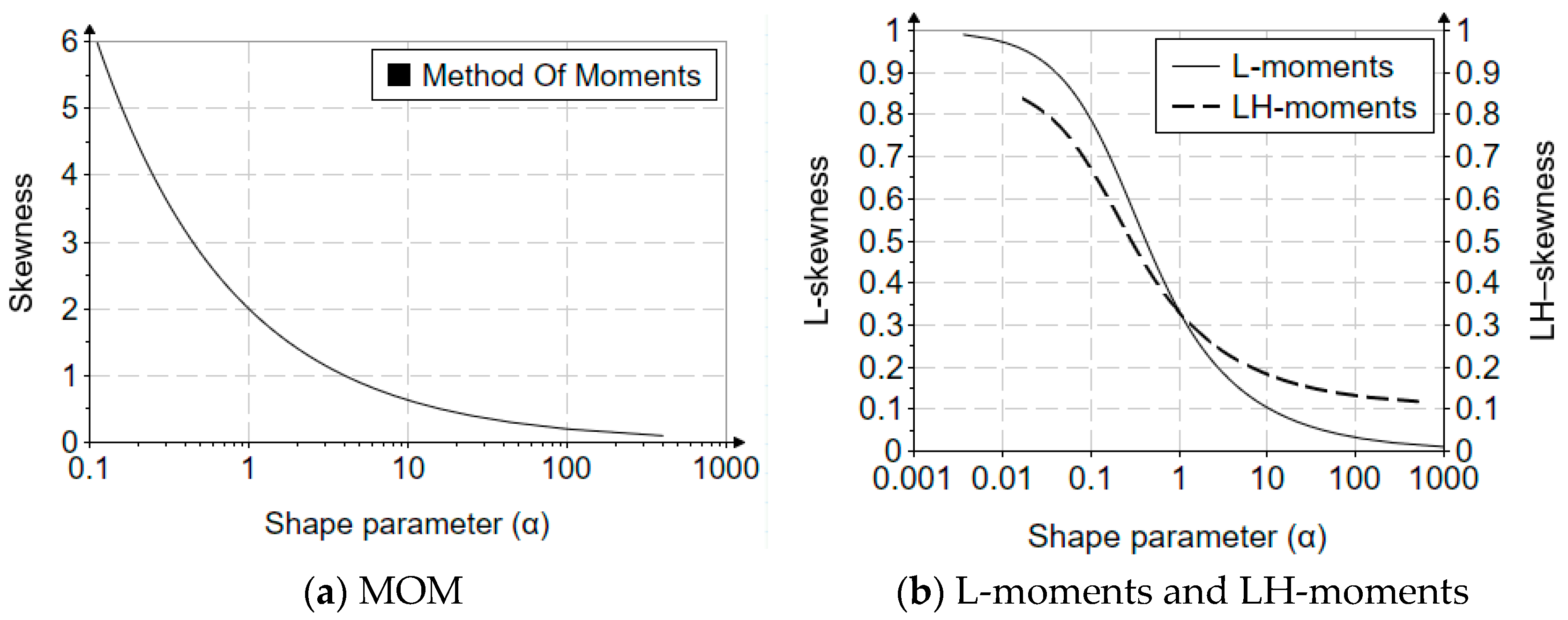
Figure 2 shows variation graphs of the shape parameter. Its determination, exact or approximate (approximation relations or even graphically), leads to the establishment of the values of the scale and shape parameters. In the case of MOM, the skewness definition range was chosen to be 0.1–6. In the case of the L-moments method, the L-skewness is chosen to be between 0–1, respectively, and 0.1–0.85 in the case of the LH-moments method. In both representations, the parameter values are on a logarithmic scale.

2.3.1. Method of Ordinary Method (MOM)

In general, the method directly computes sample moments (mean, variance, and skewness) using closed-form expressions, making it computationally efficient and fast.
For a given theoretical distribution, the four conditions are obtained based on the centered or uncentered moments of the distribution, through equivalence relations. The raw moments can be expressed using the probability density function or the quantile function, as follows ( r 1 ):
m r = E x r = x r f x d x = 0 1 x p r d p
The term of the r-th order cumulant of the Pearson III distribution, which generates moments, has the following expression:
g r = β r Γ α Γ α + r
Based on these, the centered moments are determined as follows:
m 1 = μ = γ + g 1 = γ + β α
m 2 = σ 2 = g 2 g 1 2 = α β 2
m 3 = g 3 3 g 2 g 1 + 2 g 1 3 = 2 α β 3
m 4 = g 4 4 g 3 g 1 + 6 g 2 g 1 2 3 g 1 4 = 3 α β 4 α + 2
m 5 = g 5 5 g 4 g 1 + 10 g 3 g 1 2 10 g 2 g 1 3 + 4 g 1 5 = 4 α β 5 5 α + 6
m 6 = g 6 6 g 5 g 1 + 15 g 4 g 1 2 20 g 3 g 1 3 + 15 g 2 g 1 4 5 g 1 6 = 5 α β 6 3 α 2 + 26 α + 24
Skewness:
γ 1 = C s = m 3 m 2 3 / 2 = 2 α
Kurtozis:
γ 2 = C k = m 4 m 2 2 = 6 α + 3
The distribution parameters’ expressions for MOM estimation are as follows [6,11]:
α = 2 C s 2
β = σ 2 C s
γ = μ α β
Based on the origin of the maximum flows and the coefficient of variation (Romanian methodology), Figure 3 presents the variation graphs of the parameters.

2.3.2. Linear Moments (L-Moments)

L-moments involves ordering data (rank statistics) and calculating linear combinations of order statistics, adding a sorting step but remaining relatively efficient (see Appendix C).
Using the quantile of the function and the equations, the exact parameter estimate for the L-moment technique is carried out numerically (definite integrals). Using the Gaussian quadrature method, the integrals are numerically determined. But, an approximate form of parameter estimation can be adopted because the third L-moments ( L 3 ) and L-skewness ( τ 3 = L 3 / L 2 ) depend only on the shape coefficient.
The selection of approximation functions was guided by a graphical analysis of the slope variations, supported by first-order derivatives.
When variations were uniform over specific intervals, the appropriate function type was chosen:
(a)
For uniform variation on a logarithmic scale, the function’s argument was logarithmized, and a polynomial function was used;
(b)
For non-uniform logarithmic variation, a rational function—the ratio of two polynomials—was applied, sometimes simplifying to a polynomial.
Depending on the probability distribution, either a single function type (rational or polynomial) was used across the entire range, or both were applied to different intervals. The optimal functions balanced the relative error and the complexity, minimizing error with a reasonable number of terms. Calibration was conducted using linear least squares for polynomial functions and nonlinear least squares for rational functions.
So, depending on the positive domain of L-skewness ( τ 3 ), it is possible to approximate the shape parameter using three exponential functions:
if 0 < τ 3 1 3 :
α = exp 2 . 125807169 1 . 931814923 ln τ 3 + 0 . 003031514 ln τ 3 2 0 . 004126925 ln τ 3 3 0 . 000614577 ln τ 3 4
if 1 3 < τ 3 2 3 :
α = exp 3 . 221310887 4 . 891656359 ln τ 3 2 . 771799966 ln τ 3 2 0 . 900989941 ln τ 3 3
if 2 3 < τ 3 < 1 :
α = exp 6 . 519713 92 . 299347 ln τ 3 1141 . 511558 ln τ 3 2 7840 . 37522 ln τ 3 3 28702 . 195627 ln τ 3 4 52774 . 286034 ln τ 3 5 38296 . 859615 ln τ 3 6
Another approximation relation was proposed by Hosking and Wallis [9].
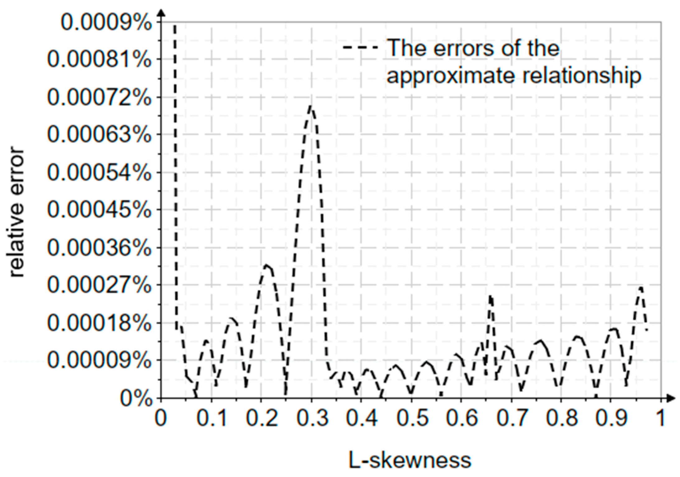
Figure 4 shows the relative errors in parameter estimation as a function of L-skewness ( τ 3 ).
With the known α , the scale parameter β and the position parameter γ are determined with the following expressions [9]:
β = L 2 π Γ α Γ α + 1 2
γ = L 1 α β
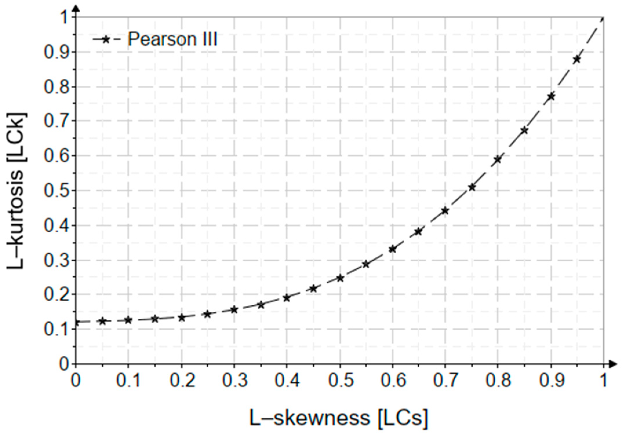
An important aspect, characteristic of the L-moments method, is represented by the relationship and variation diagram of L-kurtosis depending on L-skewness; these constitute important elements in choosing the best model when several statistical distributions are analyzed. For the Pearson III distribution, the τ 4 τ 3 dependency relationship is:
τ 4 τ 3 = 0 . 1217175 + 0 . 030285 τ 3 + 0 . 0266125 τ 3 2 + 0 . 8774691 τ 3 3 0 . 0564795 τ 3 4
Figure 5 shows the variation of L-kurtosis depending on the positive L-skewness, obtained with the L-moments method.

2.3.3. High-Order Linear Moments (First Level LH-Moments)

The LH-moments method extends L-moments by weighting higher-order moments, slightly increasing the computational cost but maintaining logarithmic dependence due to sorting.
Like the L-moments method, exact equations are obtained from solving a system of nonlinear equations using defined integrals. And for this method, LH-skewness is characterized only by the shape parameter. Thus, it was possible to obtain approximate relations for estimating this parameter, giving values for LH-skewness. Thus, for the LH-moments method, α can be approximated with the next relation:
if 0.12 < τ H 3 0.34 :
α = exp 2157 . 6573 9974 . 5911 ln τ H 3 19623 . 0505 ln τ H 3 2 21289 . 0883 ln τ H 3 3 13756 . 8891 ln τ H 3 4 5297 . 0892 ln τ H 3 5 1125 . 8409 ln τ H 3 6 101 . 9504 ln τ H 3 7
if 0.34 < τ H 3 0.85 :
α = exp 7 . 9731 34 . 552 ln τ H 3 86 . 8945 ln τ H 3 2 120 . 3149 ln τ H 3 3 82 . 8477 ln τ H 3 4 22 . 5386 ln τ H 3 5
β = 2 L H 2 3 z 1
γ = L H 1 2 β z 2
where z 1 = 0 1 q g a m m a p , α 3 p 2 2 p d p , which can be approximated with the following equation:
z 1 = 0 . 00315255 + 0 . 87292281 α + 0 . 18314623 α 2 1 + 2 . 01526823 α + 0 . 07089912 α 2 0 . 00034641 α 3 + 0 . 00000094 α 4
and z 2 = 0 1 q g a m m a p , α p d p , which can be approximated with the following equation:
z 2 = 0 . 01180195 + 0 . 87724953 α + 0 . 46798927 α 2 + 0 . 01808637 α 3 + 0 . 00004649 α 4 1 + 0 . 80457526 α + 0 . 03470298 α 2 + 0 . 0000921 α 3
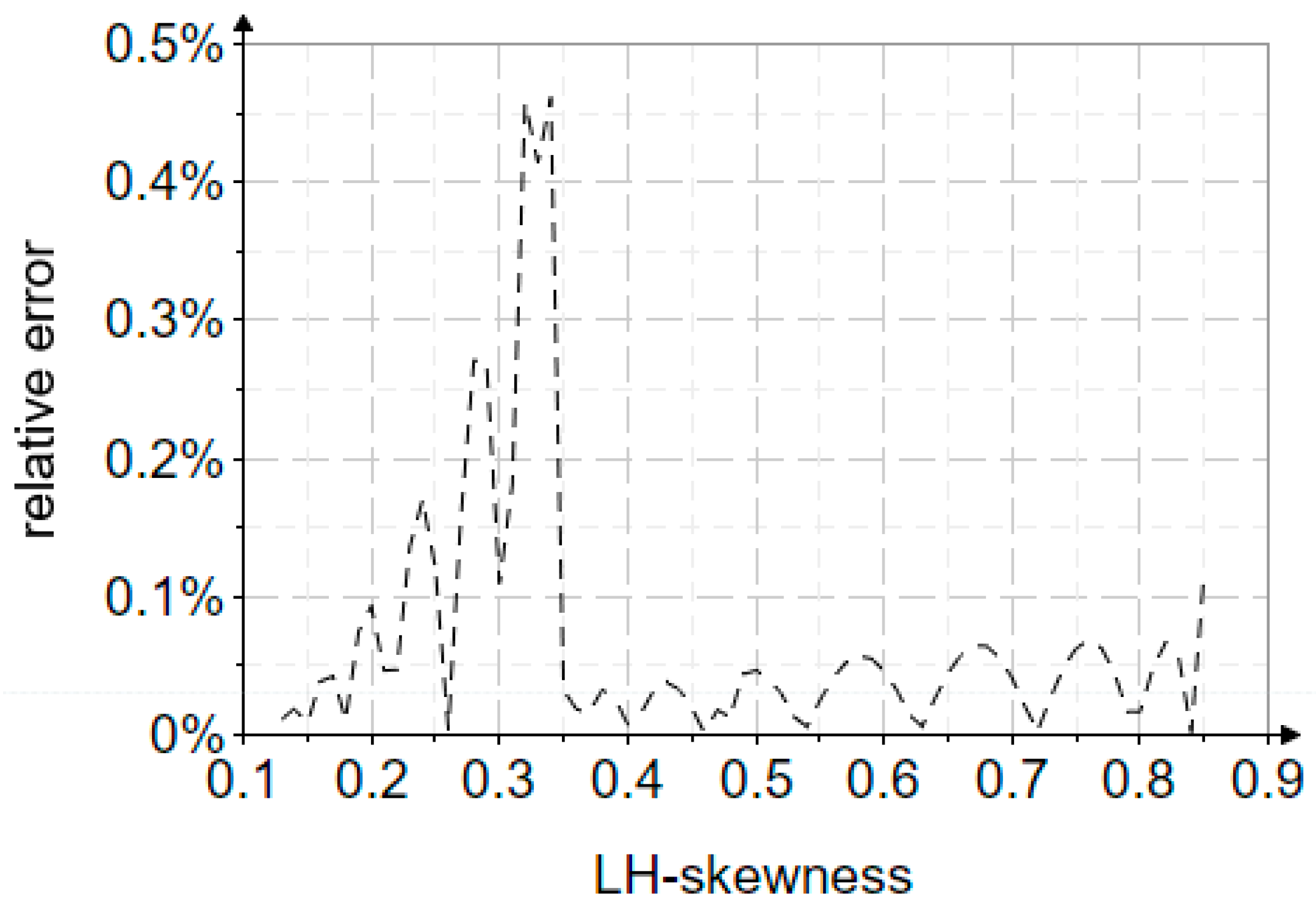
Figure 6 shows the relative errors in parameter estimation depending on LH-skewness ( τ H 3 ).
As in the case of the L-moments method, this method is also based on the values of the two higher-order indicators in choosing the best model. The τ H 4 τ H 3 dependency relationship is:
τ H 4 τ H 3 = 0 . 1012322 0 . 2437927 τ H 3 + 3 . 5538482 τ H 3 2 13 . 8996553 τ H 3 3 + 31 . 3422272 τ H 3 4 35 . 5781144 τ H 3 5 + 20 . 677076 τ H 3 6 4 . 8315272 τ H 3 7
Figure 7 shows the variation of LH-kurtosis depending on the positive LH-skewness, obtained with the LH-moments method.

2.3.4. Maximum Likelihood Estimation (MLE)

The MLE is a straightforward approach for estimating the parameters of a theoretical distribution. It involves taking the logarithm of the objective function, defined as the product of the probability density function, and then deriving it with respect to the distribution parameters.
-
Objective function:
L = i = 1 n f x i , α , β , γ = i = 1 n x i γ α 1 β α Γ α exp x i γ β
-
Logarithm of the objective function:
ln L = ln i = 1 n f x i , α , β , γ = i = 1 n ln f x i , α , β , γ = i = 1 n ln x i γ α 1 β α Γ α exp x i γ β
By differentiating the logarithmic objective function of the PE3 and minimizing it, a system of nonlinear equations is obtained, leading to the determination of the position parameter, γ [6,28]:
ψ 1 n i = 1 n Q i γ 1 n i = 1 n Q i γ 1 1 n i = 1 n 1 Q i γ = 1 n i = 1 n ln Q i γ 1 n i = 1 n Q i γ 1 1 n i = 1 n 1 Q i γ
With the parameter γ known, the shape and scale parameters are determined with the following relations:
β = 1 n i = 1 n Q i γ 1 1 n i = 1 n 1 Q i γ
α = 1 n i = 1 n Q i γ β

2.3.5. Least Squares Method (LSM)

The LSM is a less commonly used method due to its lack of robustness in parameter estimation. However, it can serve as an initial estimation tool, providing kernel values for gradient-based methods. This approach relies on the cumulative function of the theoretical distribution [6,28].
The corresponding equations for PE3 are as follows:
i = 1 n Γ α , x γ β Γ α P e i Γ α , x γ β Γ α α = 0
i = 1 n Γ α , x γ β Γ α P e i Γ α , x γ β Γ α β = 0
i = 1 n Γ α , x γ β Γ α P e i Γ α , x γ β Γ α γ = 0
where P e i represents the chosen empirical probability. The influence of the chosen empirical probability can, thus, be observed, thus leading to a subjective nature of the analysis.

2.4. The Theoretical Framework Regarding the Influence of the Analyzed Data Lengths on the Behavior of the Pearson III Distribution

The variability in the length of recorded data plays a crucial role in determining extreme maximum values in hydrology, particularly in the frequency analysis of peak flows. Since frequency analysis aims to achieve results with minimal uncertainty, the length of the analyzed data significantly influences accuracy. Short- and medium-length data series tend to exhibit increasing relative errors as the annual exceedance probability decreases. The rarer the event, the higher the relative errors (bias), which are also affected by the intrinsic characteristics of the analyzed distribution and the method used for parameter estimation.
This section examines the influence of data length variability on extreme value estimation, focusing specifically on the MOM and L-moments. These two methods are widely used in hydrological frequency analysis due to their reliance on key statistical indicators. MOM is based on traditional statistical moments, such as the arithmetic mean, coefficient of variation, skewness, and kurtosis. In contrast, L-moments utilize linear combinations of ordered data, characterized by L-moment analogs: expected value, coefficient of L-variation, L-skewness, and L-kurtosis.
These methods are chosen for analysis not only because they provide robust statistical estimations but also due to their extensive application in regional extreme event studies. MOM remains a fundamental approach in parameter estimation, while L-moments offer advantages in cases of small sample sizes or distributions with heavy tails. By comparing these two techniques, this section highlights their strengths, limitations, and the extent to which data length variability impacts their accuracy in hydrological applications.
The analysis focuses on quantifying the deviations that arise due to the influence of the size of the analyzed data sets. Given that flood frequency analysis is primarily concerned with estimating rare and very rare quantiles, special attention is given to the maximum flow corresponding to an annual exceedance probability of 0.01% (equivalent to an average return period of 10,000 years). The determination of this value is crucial for verifying the safety of class 1 retention dams, as required by hydrotechnical regulations [48,49].
In general, identifying deviations from the theoretical distribution curve is a subsequent step in the process of selecting the best-fit probability distribution. This ensures that the analyzed dataset is representative of the chosen distribution, providing greater confidence in the results. For the MOM, deviations are analyzed based on the typical values of the coefficient of variation commonly encountered in extreme hydrological event studies. The skewness coefficient is determined using three multiplication factors, selected according to the genesis of maximum flows, following standard Romanian hydrological practice [13]. Furthermore, this analysis highlights the impact of dataset length on the precision of estimated quantiles, emphasizing the differences between theoretical and empirical distributions.
By assessing these deviations, the study aims to provide insights into the reliability of extreme value estimates and their implications for hydrological design and risk assessment in dam safety evaluations.
For the L-moments method, biases are analyzed across the entire matrix of theoretical values for the L-skewness and L-kurtosis indicators, with L-skewness generally considered positive. The coefficient of L-variation (L−CV, τ 2 ) always takes values between 0 and 1, while the limits for L-skewness and L-kurtosis range within 2 τ 2 1 τ 3 < 1 , respectively, 1 4 5 τ 3 2 1 τ 4 < 1 [6].
The procedure for determining biases consists of several key steps aimed at evaluating the impact of sample size on parameter estimation accuracy in hydrological frequency analysis. First, theoretical values for the relevant indicators are selected, ensuring that they represent a broad range of distributional characteristics. Next, the parameters of the corresponding probability distributions are estimated based on these theoretical values. Once the distributions are defined, a resampling technique is applied to generate multiple samples, allowing for the recalculation of the indicators across different dataset sizes. To simplify the bias evaluation process, the expected value ( μ ) is chosen. By analyzing the deviations between these values, the study provides insights into how biases evolve as a function of sample size, offering a clearer understanding of the reliability of different parameter estimation methods.
Additionally, this methodology helps to assess the extent to which sample size influences the stability of methods in hydrological applications, particularly for extreme event analysis.
In the sampling process, after estimating the distribution parameters and determining the theoretical values of the inverse function, the Hazen empirical probability is used. This choice is based on its suitability for the two selected distributions and estimation methods, as it ensures that biases at all three levels—indicators, parameters, and quantiles—exhibit the smallest deviations from the theoretical values.
Biases are expressed as percentages. A positive bias indicates that the calculated sample values are lower than the theoretical population values, requiring an increase by the given percentage. Conversely, a negative bias means the sample values are higher than the theoretical ones and should be reduced accordingly.
The sampling analysis is conducted using representative data lengths and rare-to-very rare quantiles to ensure the relevance of the analysis domain. The theoretical values of the statistical indicators, based on the estimation methods, are selected to be both common and relevant for this type of analysis.
Table 3, Table 4, Table 5, Table 6, Table 7 and Table 8 present the impact of data length variability on the statistical indicators, parameters, and quantiles, assuming that the data are drawn from a Pearson III distribution. For MOM, the approach in determining asymmetry follows the methodology from Romania.
Considering that various regimes with different variabilities can be encountered in practice, Table 9 and Table 10 present the biases of the Pearson III distribution for MOM and for the L-moments method. These tables cover the full matrix of statistical indicators and the rarest event, Q0.01%. It is observed that, for MOM, the biases are significant in cases of medium and high variability and skewness, whereas the biases for the L-moments method are very small.
Figure 8 provides a clear and detailed graphical representation of the steps involved in the flood frequency analysis, including distribution selection, parameter estimation methods, model validation, and practical applicability.

3. Case Studies

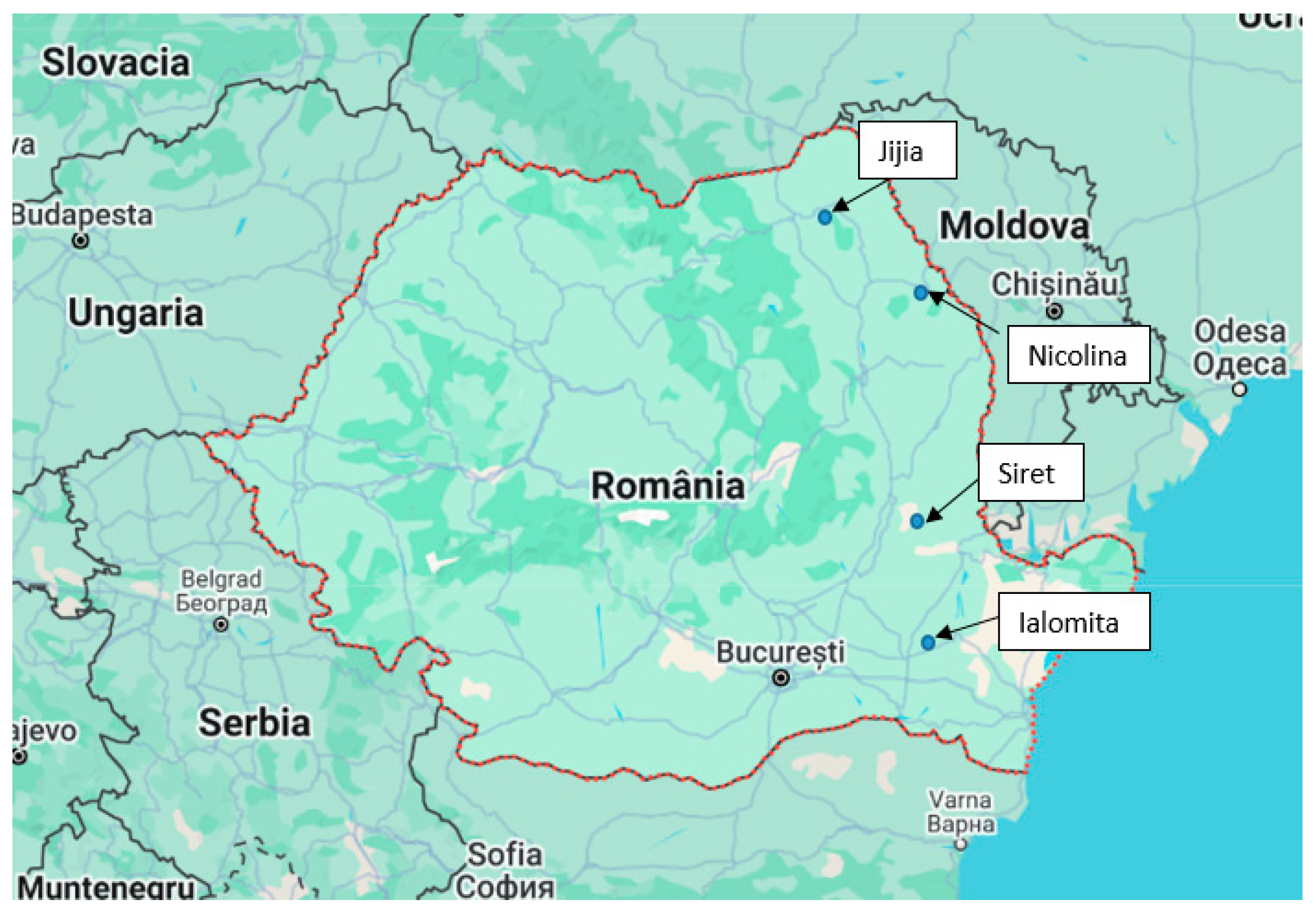
As case studies, the frequency analysis of the maximum flows on four rivers (the Ialomita, Siret, Jijia, and Nicolina) with different morphometric and statistical characteristics is carried out. Figure 9 shows the locations of the four monitoring stations.

3.1. Description of the Analyzed Rivers Morphometric Information

3.1.1. Ialomita River

The Ialomita River (cadastral code XI) is a left tributary of the Danube River. Located in Southern Romania, it has a total length of 417 km, a river basin area of 10,350 km2, an average slope of 15%, an average altitude of 327 m, and a sinuosity coefficient of 1.88. The Tandarei station is located around 20 km upstream from the Danube River confluence. The climate is temperate continental, with precipitation ranging between 410 and 510 mm per year.

3.1.2. Siret River

As the left tributary of the Danube River, the Siret River (cadastral code XII) is situated in the northeastern region of Romania. With a length of 647 km, the dependent Siret river system springs from the Woody Carpathians of Ukraine; 559 km (the Middle and Lower Siret) of the entire length are located inside Romanian borders. At 42,890 km2, or around 18.1% of the country’s surface, it is the largest hydrographic basin in Romania.
The region experiences a mild continental climate; the multiannual average precipitation falls from 800–1000 L/m2 in the high mountain region to 450–550 L/m2 in the plain region. The river’s altered regime is a result of several retention projects, which affect the maximum yearly values.

3.1.3. Jijia and Nicolina Rivers

The Jijia River (cadastral code XIII.1.15) rises in the Hiliseu–Horia locality of Botosani and is a tributary of the Prut River (cadastral code XIII, spring from the Woody Carpathians of Ukraine). Being a tributary of the River Jijia, the Nicolina River is a component of its hydrographic basin. The rivers are situated in the eastern region of Romania, oriented roughly northeast, at 47°55′59.6″ N 26°24′17.1″ E.
The Prut–Barlad hydrographic space has a temperate continental climate. Multiannual averages of 400 to 600 mm of precipitation each year are stated in terms of precipitation. The monitoring stations are arranged to allow for a natural maximum reported flow regime.
The morphometric characteristics of a watershed not only influence the hydrological response but also condition the statistics of the recorded peak flows. This, in turn, determines the shape of the probability distribution that describes the behavior of extremes.
Particularly in regional modeling, the relationship between morphometry, moments, and parameters is essential for coherent and physically justified estimates.
Therefore, it is necessary to present all of this relevant information (see Table 11) that is characteristic of peak flow frequency analyses.

3.2. Time Series of Maximum Annual Flows

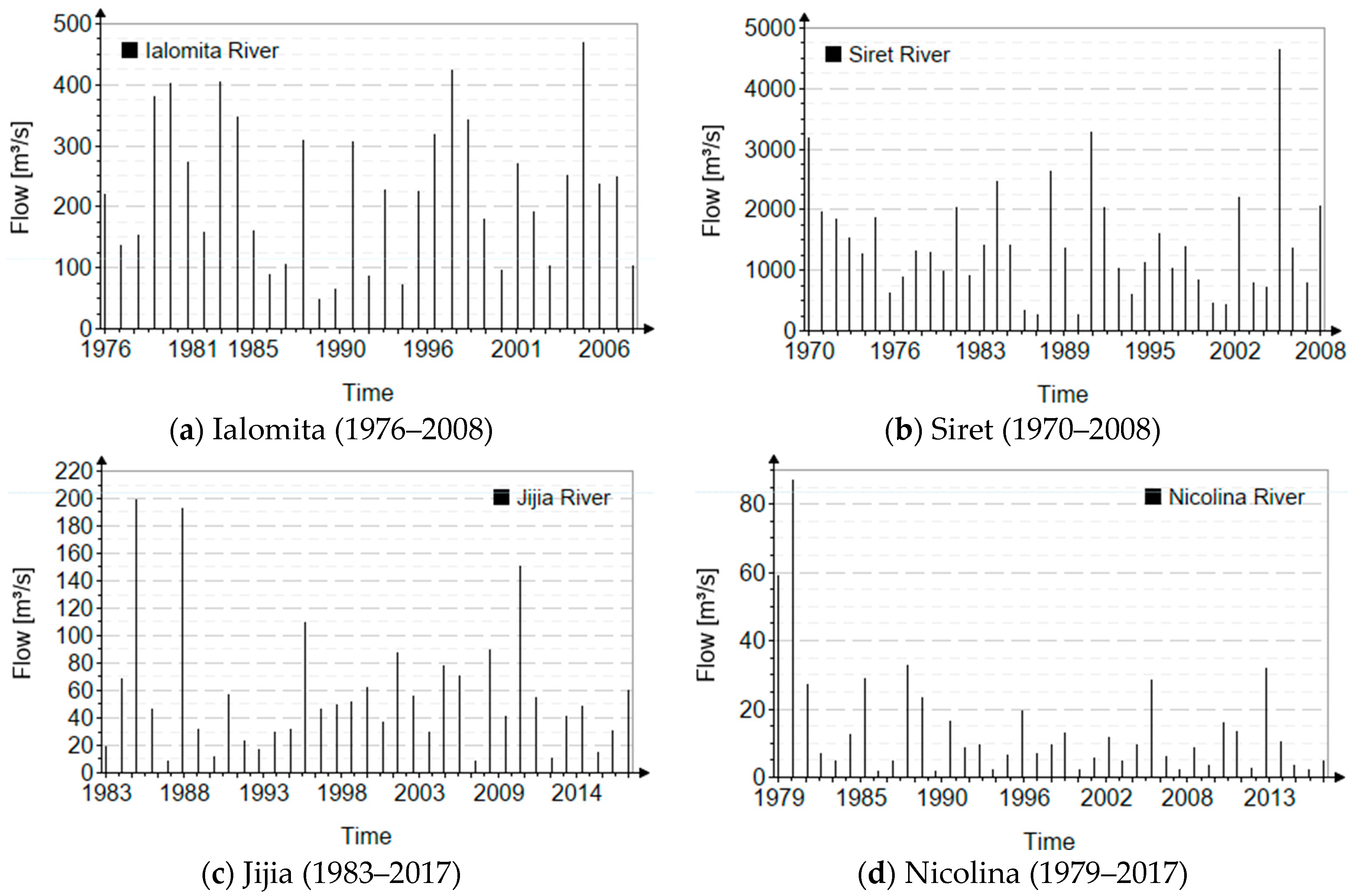
Figure 10 shows the chronological series of the maximum annual flows related to the analyzed case studies.
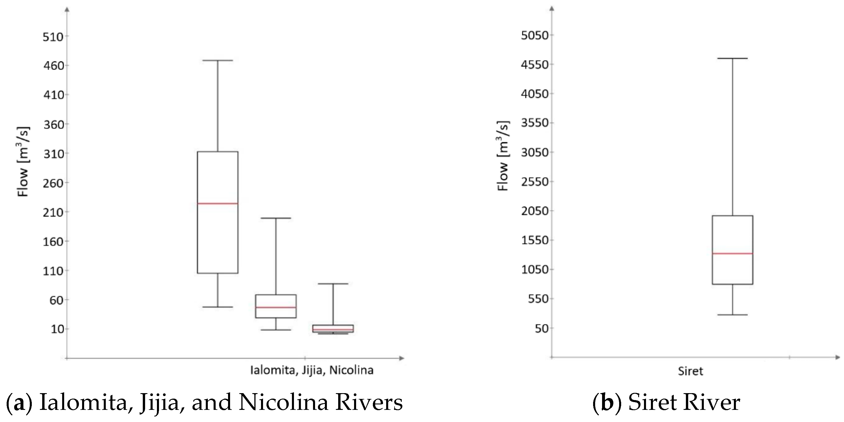
The graphic representation of the most important statistical characteristics (25%, median: 50%, and 75% quartiles; the minimum and maximum values of the data that are not outliers) is represented in the box-plot graphs of Figure 11.
Table 12 and Table 13 list the statistical indicator values for the examined data sets, including the expected value ( μ ), coefficient of variation ( C v ), skewness ( C s ), coeficientul de L-variatie ( τ 2 ), L-skewness ( τ 3 ), LH-skewness ( τ H 3 ), L-kurtosis ( τ 4 ), and LH-kurtosis ( τ H 4 ).
In the case of the analysis using MOM, the skewness is chosen according to the genesis of the flows by multiplying the coefficient of variation ( C v ) of the analyzed data with a coefficient ( ξ ) that reflects this genesis (the values of this coefficient were presented in the Section 1).
The homogeneity of the observed data was checked with the help of the Von Newman statistical test, with all analyzed series being homogeneous and the test results being in each case greater than two, which represents the minimum threshold value characteristic of the von Neumann test [51]. The stationarity condition was performed using the “t” test [51]. All the observed data are stationary. Using the Grubbs test [2,3,51], the possible presence of outlier values was checked for both tails. No outliers were identified.

4. Results and Discussions

The objective of the analysis is to evaluate the performance of the methods presented here in forecasting quantile values for rare and very rare events. Given the focus on quantile values of interest, the results presented will be based on this criterion.
In the frequency analysis of extreme events, and especially in the frequency analysis of maximum flows, the most important problem is the choice of the best model, because in the field of these small annual exceedance probabilities, the upper tails of the distributions have different behaviors being influenced by various factors such as the available length of the analyzed string, by the statistical characteristics of the analyzed data (coefficient of variation, skewness, and kurtosis) by particular aspects specific to the analyzed distributions (if they have an upper bound, if they present special cases, the number of parameters, characteristics regarding the family it belongs to (light tailed, heavy tailed), and last but not least, the parameter estimation method). As previously mentioned, in the case of parameter estimation methods (the method of least squares and the method of weighted moments), an important role is played by the choice of the empirical probability.
Thus, the discussions regarding the analysis in this manuscript will be focused on the behavior of the Pearson III distribution on this field of probabilities, on the particular forms of the upper tail of the quantile function, on the values generated by the different methods of estimating the parameters used, and most importantly, on the methods of estimation recommended following the analysis regarding the stability and robustness related to the different statistical–hydrological scenarios. This implies highlighting a robust criterion for selecting the best model, as well as presenting a confidence interval of the best model, which is statistically accessible. For the plotting positions, the Hazen formula [8] was used ( P = i 0.5 / n ). The probability axis is represented on a logarithmic scale.
A confidence interval is constructed for L-moments using the Chow approximation [2,6,8,14] defined for a 90% confidence level (10% significance level). This approach considers the confidence interval as a variable function dependent on the probability and specific standard error associated with each statistical distribution [6,14].
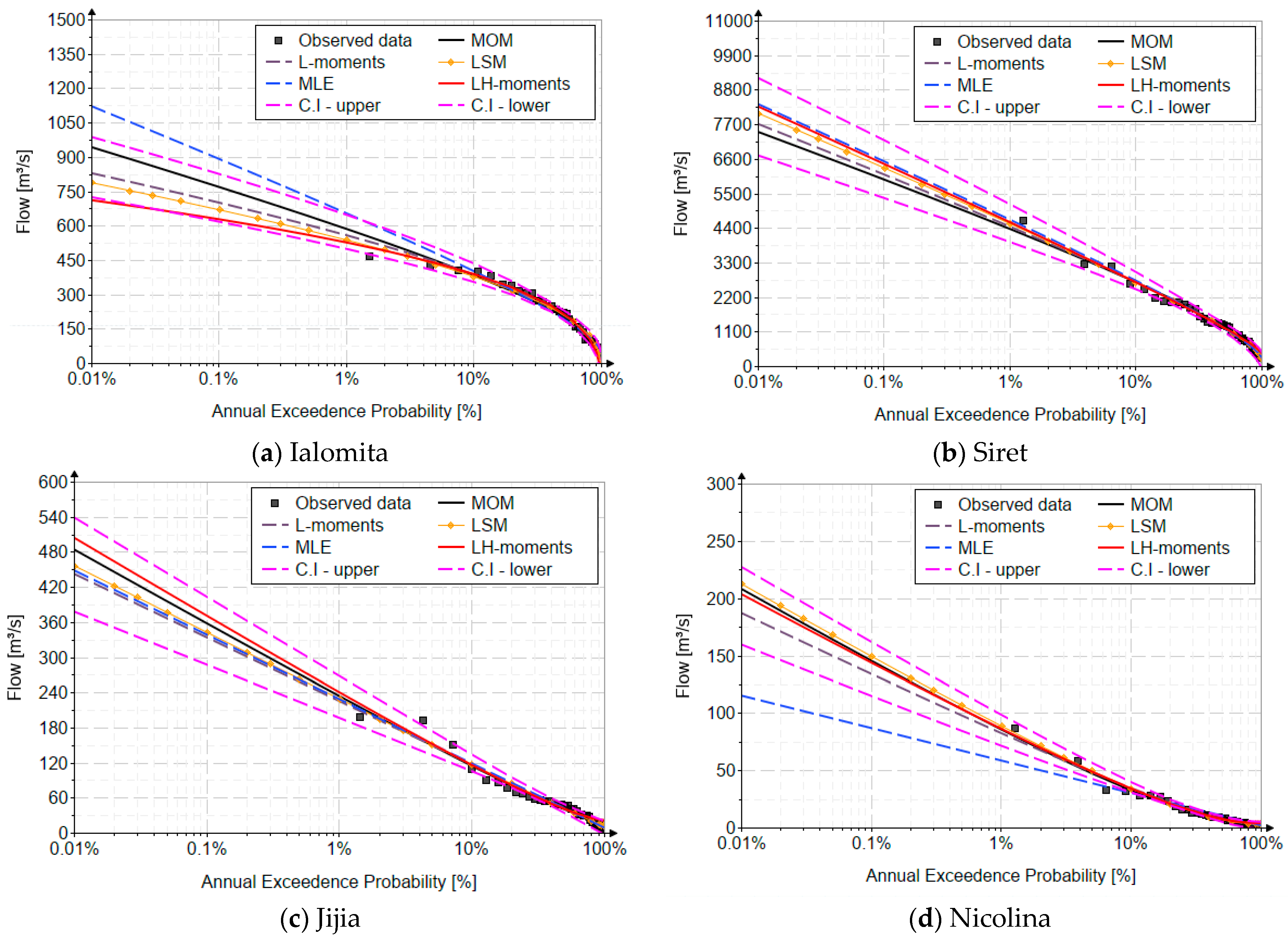
Figure 12 shows the results obtained for the case studies using the five analyzed estimation methods, as well as the confidence interval for the L-moments method.
Upon analyzing the results obtained, it becomes evident that, for data series exhibiting skewness greater than two (e.g., Nicolina), the maximum likelihood method fails to converge, resulting in quantile values characterized by significant errors. These errors escalate with higher skewness values. For this case study, the generated values are much underestimated, 115 m3/s, with values much lower than those generated with the method L-moments, considered a reference due to its stability and robustness, namely 187 m3/s.
In the case of MOM, the resulting values are notably influenced by the short length of the data series. This dependency stems from the method’s characteristics, where errors increase proportionally with higher statistical indicators that require calibration, such as variance and skewness. Additionally, establishing skewness based solely on flow genesis, without a thorough analysis, introduces subjectivity into the assessment, which is a significant drawback. These errors are further pronounced when applying simplified approaches for basins larger than 100 km2, where a uniform variation coefficient of one and a multiplication coefficient of four are typically used. To illustrate, the curves corresponding to these coefficients for the Siret river are presented for comparison.
Subjectivity also arises in the least squares method, where many researchers adopt a predefined empirical probability like the Weibull probability, leading to notable deviations. The choice of empirical probability should align closely with the estimation method and the distribution’s nature. Recent studies [8] have made a significant discovery in addressing this issue, highlighting that the Hazen empirical probability yields the smallest deviations from theoretical values in the Pearson III distribution.
In all case studies, the values generated by MOM are relatively close to those generated by the L-moments method, but with the important mention that the skewness was imposed on the rationales described previously, but whose choice is not recommended, as it can be easily influenced by subjective aspects (see Figure 12). The values obtained with MOM are 942 m3/s (Ialomita river), 7454 m3/s (Siret river), 484 m3/s (Jijia river), respectively, and 208 m3/s (Nicolina river), values close to those obtained with the reference L-moments method, namely 829 m3/s (Ialomita river), 7706 m3/s (Siret river), 442 m3/s (Jijia river), respectively, and 187 m3/s (Nicolina river).
In the case of the LSM method, it generates values close to those obtained with MOM and L-moments, but it must be used with reservations. The LSM method is a method also influenced by subjective aspects in choosing the empirical probability, leading to errors as high as 8% when using Weibull plotting positions instead of Hazen’s. Among the five methods examined, the L-moments method emerges as the recommended choice due to its stability and robustness, particularly suitable for short data lengths. The L-moments method consistently produces quantile estimates with minimal bias, especially for short data series, with relative errors below 5% for most cases. For the Siret River, quantile values using L-moments were 7706 m3/s, while MOM produced 7454 m3/s, a deviation of about 3.3%. For the Jijia River, L-moments yielded 442 m3/s versus MOM’s 484 m3/s, a 9.5% overestimation. These differences underscore the necessity for robust parameter estimation methods, especially when handling extreme events. Alongside the LH-moments method, it is distinguished by having clear selection criteria, specifically the calibration of higher-order linear moments, supported by approximate relationships and graphical representations of these indicators. The LH-moments method serves as an alternative to frequency analysis with partial series (peak over thresholds or annual exceedance series), utilizing the series of maximum annual flows. This approach mitigates the drawback of the block maximum/annual maximum method, which sometimes includes non-flood maximum values. LH-moments method provides slightly larger quantiles compared to L-moments, particularly for highly skewed distributions, emphasizing its usefulness in complementing partial series analysis.
A crucial aspect of the analysis is the statistical significance of the results and the associated confidence intervals. For L-moments, confidence intervals were constructed using Chow’s approximation at a 90% confidence level. These intervals, shown graphically, demonstrate that, (a) for the Ialomita River, the 90% confidence interval for the 0.01% quantile ranges from 790 m3/s to 870 m3/s, with the point estimate at 829 m3/s. (b) For the Siret River, the 0.01% quantile spans from 7500 m3/s to 8000 m3/s, bracketing the 7706 m3/s point estimate. Broader intervals were observed for rivers with higher skewness, such as the Nicolina, due to greater uncertainty in parameter estimation. These intervals highlight the importance of accounting for uncertainty when forecasting extreme flows, as narrow intervals may give a false sense of precision.
Thus, following the comparative analysis, the most important and relevant observations are:
(1)
It is recommended to abandon the MOM, especially to use it while using the artificial choice of skewness. In this way, the strong subjective character that currently dominates the frequency analysis of maximum flows is eliminated. This also presents the disadvantage of some important theoretical biases, especially for short data series;
(2)
It is recommended to use the PE3 distribution using the L-moments method, and only after a pre-selection stage based on the L-skewness and L-kurtosis values and interdependence diagrams. It is very important that, in the second stage, the biases of the distribution depending on the length of the observed data should be highlighted. For example, a short data series (25 years) for Nicolina resulted in biases of up to 31% for the 0.01% quantile. Longer series (50–80 years) reduced biases significantly, with errors under 5% for the Ialomita and Siret Rivers. Draw the confidence interval that includes these theoretical uncertainties.
It is crucial to emphasize that the entire analysis assumes the Pearson III distribution as the “parent” model, as currently practiced and recommended by flood frequency analysis in Romania. However, this approach should be reconsidered, advocating for the adoption of the L-moments method as the standard approach. The selection of the optimal distribution (both at-site and regional) should then be based on criteria specific to this method. This includes ensuring that the chosen distribution effectively calibrates the higher-order statistical indicators (L-skewness and L-kurtosis) of the analyzed datasets as accurately as possible. This revised approach is essential to prevent the forecasting of underestimated or overestimated maximum values, which could have adverse consequences.
Thus, based on these rigorous principles, and taking into account the values of the statistical indicators of the data analyzed for the four case studies, respectively, the graphs and interdependence relationships of these indicators [7,9,10,40], the best three parameter distributions would be represented by Pareto distribution for the Ialomita River; the log-normal distribution or GEV distribution for the Siret River; log-logistic or inverse paralogistic distributions for the Jijia River, and log-normal distribution for the Nicolina River.
But, taking into account the results obtained in previous materials, it is recommended to use as a “parent” distribution a four-parameter distribution, namely the Wakeby or Burr distribution, which precisely calibrates these statistical indicators. These have the disadvantage of requiring special attention in the calibration of the parameters, as it is necessary to solve a system of four nonlinear equations.

5. Conclusions

The Pearson III distribution is widely employed in FFA. However, in Romania, there is a common misuse of this distribution, particularly for basins larger than 100 km2. Often, it is inaccurately applied with approximations that assume a skewness of four. This approximation is derived by multiplying a chosen coefficient of variation (typically one) by another coefficient (typically four), which is based on the assumption that large flow events stem solely from precipitation.
The Pearson III distribution is particularly well-suited for extreme event analysis due to its flexibility, making it ideal for hydrological data, which often exhibit significant skewness. The distribution effectively captures the behavior of extreme values, which is crucial for predicting peak flows with very low exceedance probabilities (e.g., 0.01%).
The analysis results highlight that L-moments are the most stable and robust method, less affected by data length variations and outliers, offering clear criteria for selecting optimal distributions by calibrating higher-order indicators. Among the five methods examined, the L-moments method emerges as the recommended choice, as it produces quantile estimates with minimal bias, especially for short data series, with relative errors below 5% for most cases.
The LH-moments method shows similar advantages, addressing the “separation effect” by distinguishing maximum flows from annual series, akin to partial series analysis. The Pearson III distribution is unsuitable for skewness values above two when using MLE. The MOM is recommended for large datasets with minimal skewness adjustment, but assuming a fixed skewness of four should be avoided for watersheds over 100 km2, as the MOM tends to systematically overestimate flows, especially for mixed-origin flows. When using the Pearson III distribution with LSM, the Hazen empirical probability is preferred, as it produces minimal bias compared to theoretical values.
Due to the limited number of records available in many cases, the variability in recorded data lengths influences the probability distributions to varying extents, depending on the chosen parameter estimation method. According to the findings, the L-moments method shows the least susceptibility to this variability, demonstrating significantly smaller biases across the entire theoretical framework of statistical indicators compared to MOM.
Therefore, it is essential to account for these deviations from theoretical values by including the confidence interval of the chosen best-fit distribution in FFA. A practical approach is to visualize the confidence interval using Chow’s approximation, which has the added advantage of recent adaptations for the L-moments method.
Comparing the results from the current case studies with previous findings [8,40,41] underscores the critical importance of correctly utilizing the PE3. This emphasizes the value of employing the L-moments method, particularly in scenarios with limited data availability.
An important aspect is the replicability of the proposed methodology, which makes it valuable for hydrologists and engineers in other countries, especially in regions where access to long data series is limited and where an accurate estimation of extreme values is essential for the design of hydraulic infrastructure.
All this information represents a solid basis for approaching an analysis involving machine learning, both in the estimation of parameters and in the analysis regarding the selection of the best statistical distribution, aspects that represent future approaches.

6. Future Research

Given the influence of climate change on extreme events [52], future studies will investigate non-stationary models in which the distribution parameters vary over time.
An extension of the analysis to other river basins will be carried out to validate the findings and develop more generalized recommendations.
A future direction will also consist of combining statistical distributions with machine-learning algorithms [53] and the flow direction algorithm to better capture the complex relationships between extreme events and their climatic drivers.

Author Contributions

Conceptualization, C.-G.A. and D.I.; Methodology, C.-G.A. and D.I.; Software, C.-G.A. and D.I.; Validation, C.-G.A. and D.I.; Formal analysis, C.-G.A. and D.I.; Investigation, C.-G.A. and D.I.; Resources, C.-G.A. and D.I.; Data curation, C.-G.A. and D.I.; Writing—original draft, C.-G.A. and D.I.; Writing—review & editing, C.-G.A. and D.I.; Visualization, C.-G.A. and D.I.; Supervision, C.-G.A. and D.I.; Project administration, C.-G.A. and D.I.; Funding acquisition, C.-G.A. and D.I. All authors have read and agreed to the published version of the manuscript.

Funding

This research received no external funding.

Data Availability Statement

The original contributions presented in the study are included in the article, further inquiries can be directed to the corresponding author.

Conflicts of Interest

The authors declare no conflict of interest.

Abbreviations

FFAflood frequency analysis
MOMthe method of ordinary moments
L-momentsthe method of linear moments
LH-momentsthe higher-order linear moments
μ expected value; arithmetic mean
σ standard deviation
C v coefficient of variation
C s coefficient of skewness; skewness
C k coefficient of kurtosis; kurtosis
L 1 , L 2 , L 3 linear moments
τ 2 , L C v coefficient of variation based on the L-moments method
τ 3 , L C s coefficient of skewness based on the L-moments method
τ 4 , L C k coefficient of kurtosis based on the L-moments method
m 1 , m 2 , m 3 , m 4 central moments (with MOM)
Gamma.INVreturns the inverse cumulative probability distribution for the Gamma distribution.
In Mathcad Prime 6, this has the expression: q g a m m a p , s h a p e
In R, this has the expression: q g a m m a p , s h a p e , r a t e , s c a l e = 1
In Python, g a m m a . p p f p , s h a p e , s c a l e

Appendix A. The Frequency Factors

The frequency factor is a coefficient used in the statistical analysis of random variables to determine the quantiles of a probability distribution based on a given probability level. It is defined in relation to the mean and standard deviation of the distribution (for MOM) or in relation to the first two linear moments (for L- and LH-moments) and is essential in hydrology, meteorology, and other engineering fields for estimating extreme values.
Frequency factors are crucial in the frequency analysis of peak flows, as they are specific to each statistical distribution and are used for extrapolating extreme values based on the desired return period.
Using the frequency factor, K p , α , the inverse functions for MOM, L-moments, and LH-moments can be formulated as follows:
x p = μ + σ K M O M p , α x p = L 1 + L 2 K L p , α x p = L H 1 + L H 2 K L H p , α
where μ is the expected value and σ is the standard deviation; L 1 and L 2 are the first two L-moments; and L H 1 and L H 2 are the first two LH-moments.
The exact relationships for the frequency factors are:
K M O M p , α = G a m m a . I N V 1 p , α α α K L p , α = π Γ α G a m m a . I N V 1 p , α α Γ α + 0.5 K L H p , α = 2 3 G a m m a . I N V 1 p , α 2 z 2 z 1
where the expressions for z 1 and z 2 can be found in Section 2.3.
The frequency factor with the method of ordinary moments (MOM) can also be approximated using a polynomial development in skewness ( C s ):
K M O M p , C s = a + b C s + c C s 2 + d C s 3 + e C s 4
For the method of linear moments (L-moments), the frequency factor can be approximated using the following polynomial relation (in L-skewness, τ 3 ):
K T L p , τ 3 = a + b τ 3 + c τ 3 2
For the high-order linear moments method (LH-moments), the frequency factor can be approximated using the following polynomial relation (in LH-skewness, τ 3 H ):
K L H p , τ H 3 = a + b τ H 3 + c τ H 3 2
The coefficients of the polynomial functions, for MOM, L- and LH-moments, are presented in Appendix B.

Appendix B. The Coefficients of Approximate Functions

Table A1, Table A2 and Table A3 list the polynomial function coefficients for the annual exceedance probabilities that are utilized the most in technical hydrology.
Table A1. Coefficients of the approximation function (for MOM).
p [%]abcde
0.013.6865502.2810560.013205−0.0135750.000803
0.13.0706991.507230−0.033443−0.0067510.000475
0.52.5629160.991395−0.058405−0.0025050.000277
12.3155970.777929−0.066149−0.0008050.000200
22.0447040.571450−0.0714580.0008600.000127
31.8725110.454755−0.0732240.0018540.000085
51.6372250.313358−0.0738710.0032090.000026
101.2739930.135936−0.0719820.005620−0.000095
200.832988−0.014687−0.0667140.009667−0.000384
300.517983−0.091708−0.0540940.011752−0.000631
400.254280−0.149822−0.0275570.010103−0.000665
500.011164−0.1960260.0106080.004788−0.000449
60−0.233431−0.2199430.052175−0.002735−0.000052
70−0.501809−0.2030950.086693−0.0105140.000416
80−0.826925−0.1159020.101447−0.0163750.000831
90−1.2924450.1187580.069412−0.0163370.000986
95−1.6813440.3904220.002582−0.0094420.000734
Table A2. Coefficients of the approximation function (L-moments).
p [%]abc
0.016.588710323.442810916.3451916
0.15.476636215.5509089.0973213
0.54.565712610.21882634.7799626
14.12366337.99147893.1782715
23.64052225.82254681.7747976
33.33393684.58873461.0633868
52.91566373.08273230.3030661
102.2715641.1610927−0.4339022
201.4916395−0.5255067−0.7232427
300.9293178−1.3084367−0.6123297
400.4488931−1.6907365−0.367109
50−0.0000983−1.8093098−0.0613219
60−0.4490487−1.69691420.2698602
70−0.9293476−1.32020170.5929909
80−1.4914544−0.54097910.8375167
90−2.27111991.14882380.71406
95−2.91523753.0846318−0.0297187
Table A3. The coefficients for LH-moments (first order).
p [%]abcdefg
0.01138.4454−2465.140317,892.3121−63,752.6912120,214.5111−114,563.992543,558.7960
0.152.6867−889.81406536.4462−23,385.630644,343.2094−42,529.193416,305.2083
0.58.5283−84.4050710.0442−2635.33215249.2959−5311.16132175.4185
1−2.6280115.7398−752.64862601.1523−4681.31814213.7614−1475.0655
2−6.4948179.9173−1244.96494403.9528−8196.90427690.8402−2858.8140
3−4.9899146.9756−1028.60893668.7798−6898.55326550.0621−2473.1341
5−0.398854.1598−384.55061408.4120−2727.06092675.4512−1052.8528
103.5216−33.0494230.5684−804.89751478.4454−1366.3202491.2543
200.60222.4211−26.156073.8725−93.861527.907716.2937
30−0.44348.8140−79.7955288.7791−549.5813515.7971−185.8401
40−0.5276−1.5686−6.096238.2458−109.5742142.8124−65.6908
50−0.8662−7.338841.8998−140.8366240.5612−191.216756.2460
60−1.6664−5.008635.7882−134.5152262.9802−242.989684.4331
70−2.77161.9929−2.3618−7.374448.9529−71.180431.7503
80−3.96118.1831−33.0043110.2760−184.7844147.2649−45.4138
90−5.11856.75271.219017.2169−89.7448117.2605−49.4125
95−5.87860.313879.04519−250.3293338.36417−214.333151.2532

Appendix C. General Relations for Determining Linear Moments

To estimate the L-moments, the data set must be sorted in ascending order (Xi:n). The expressions for the first four L-moments of the data set are as follows:
  • L 1 = b 0 : the first linear moment (the arithmetic mean)
  • L 2 = 2 b 1 b 0 : second linear moment
  • L 3 = 6 b 2 6 b 1 + b 0 : third linear moment
  • L 4 = 20 b 3 30 b 2 + 12 b 1 b 0 : fourth linear moment
where b 0 , b 1 , b 2 , b 3 represent the natural estimators and have the following expressions:
b 0 = 1 n i = 1 n x i
b 1 = 1 n i = 1 n x i i 1 n 1
b 2 = 1 n i = 1 n x i i 1 n 1 i 2 n 2
b 3 = 1 n i = 1 n x i i 1 n 1 i 2 n 2 i 3 n 3
Based on these L-moments, the ratios are defined as follows:
  • τ 2 = L 2 L 1 : represents L-CV (coefficient of L-variation)
  • τ 3 = L 3 L 2 : represents L-Cs (L-skewness)
  • τ 4 = L 4 L 2 : represents L-Ck (L-kurtozis)
To estimate the parameters of a theoretical distribution (the corresponding linear moments), the expressions of the first four L-moments are obtained based on the quantile function of the distribution, as follows:
L 1 = 0 1 x ( p ) d p
L 2 = 0 1 x ( p ) 1 2 p d p
L 3 = 0 1 x ( p ) 1 + 6 p 2 6 p d p
L 4 = 0 1 x ( p ) 1 20 p 3 + 30 p 2 12 p d p

References

  1. Montanari, A.; Merz, B.; Blöschl, G. HESS Opinions: The Sword of Damocles of the Impossible Flood. Hydrol. Earth Syst. Sci. 2024, 28, 2603–2615. [Google Scholar] [CrossRef]
  2. Bulletin 17B Guidelines for Determining Flood Flow Frequency; Hydrology Subcommittee, Interagency Advisory Committee on Water Data; U.S. Department of the Interior, U.S. Geological Survey, Office of Water Data Coordination: Reston, VA, USA, 1981.
  3. Bulletin 17C Guidelines for Determining Flood Flow Frequency; U.S. Department of the Interior, U.S. Geological Survey: Reston, VA, USA, 2017.
  4. World Meteorological Organization. (WMO-No.100) 2018 Guide to Climatological Practices; WMO: Geneva, Switzerland, 2018. [Google Scholar]
  5. EM 1110-2-1415 Hydrologic Frequency Analysis, Engineering and Design; Department of the Army U.S. Army Corps of Engineers: Washington, DC, USA, 1993.
  6. Rao, A.R.; Hamed, K.H. Flood Frequency Analysis; CRC Press LLC: Boca Raton, FL, USA, 2000. [Google Scholar]
  7. Gubareva, T.S.; Gartsman, B.I. Estimating Distribution Parameters of Extreme Hydrometeorological Characteristics by L-Moment Method. Water Resour. 2010, 37, 437–445. [Google Scholar] [CrossRef]
  8. Anghel, C.G. Revisiting the Use of the Gumbel Distribution: A Comprehensive Statistical Analysis Regarding Modeling Extremes and Rare Events. Mathematics 2024, 12, 2466. [Google Scholar] [CrossRef]
  9. Hosking, J.R.M.; Wallis, J.R. Regional Frequency Analysis: An Approach Based on L-Moments; Cambridge University Press: Cambridge, UK, 1997. [Google Scholar] [CrossRef]
  10. Hosking, J.R.M. L-moments: Analysis and Estimation of Distributions using Linear, Combinations of Order Statistics. J. R. Statist. Soc. 1990, 52, 105–124. [Google Scholar] [CrossRef]
  11. Citakoglu, H.; Demir, V.; Haktanir, T. L-MOMENTLER YÖNTEMİYLE KARADENİZ’E DÖKÜLEN AKARSULARA AİT YILLIK ANLIK MAKSİMUM AKIM DEĞERLERİNİN BÖLGESEL FREKANS ANALİZİ. Ömer Halisdemir Üniversitesi Mühendislik Bilim. Derg. 2017, 6, 571–580. [Google Scholar] [CrossRef]
  12. Diaconu, C.; Serban, P. Syntheses and Hydrological Regionalization; Technical Publishing House: Bucharest, Romania, 1994. [Google Scholar]
  13. STAS 4068/1962; Maximum Water Discharges and Volumes, Determination of Maximum Water Discharges and Volumes of Watercourses. The Romanian Standardization Institute: Bucharest, Romania, 1962.
  14. Chow, V.T.; Maidment, D.R.; Mays, L.W. Applied Hydrology; MCGraw-Hill, Inc.: New York, NY, USA, 1988; ISBN 007-010810-2. [Google Scholar]
  15. Mandru, R.; Ioanitoaia, H. Ameliorative Hydrology; Agro-Silvica Publishing House: Bucharest, Romania, 1962. [Google Scholar]
  16. Bejenaru, G.; Castravet, T.; Dilan, V. Hydrological Calculations; Print Caro Publishing House: Chisinau, Moldova, 2020. [Google Scholar]
  17. Teodorescu, I.; Filotti, A.; Chiriac, V.; Ceausescu, V.; Florescu, A. Water Management; Ceres Publishing House: Bucharest, Romania, 1973. [Google Scholar]
  18. Ciupak, M.; Ozga-Zieliński, B.; Tokarczyk, T.; Adamowski, J. A Probabilistic Model for Maximum Rainfall Frequency Analysis. Water 2021, 13, 2688. [Google Scholar] [CrossRef]
  19. Nwaogazie, I.L.; Sam, M.G. Probability and non-probability rainfall intensity-duration-frequency modeling for port-harcourt metropolis, Nigeria. Int. J. Hydro. 2019, 3, 66–75. [Google Scholar] [CrossRef]
  20. Ye, L.; Hanson, L.S.; Ding, P.; Wang, D.; Vogel, R.M. The probability distribution of daily precipitation at the point and catchment scales in the United States. Hydrol. Earth Syst. Sci. 2018, 22, 6519–6531. [Google Scholar] [CrossRef]
  21. World Meteorological Organization. (WMO-No.1029) 2008 Manual on Low-Flow Estimation and Prediction; Operational Hydrology Report No. 50; WHO: Geneva, Switzerland, 2008. [Google Scholar]
  22. Institute of Hydrology. (IH) 1992 Low Flow Estimation in the United Kingdom; Report No. 108; Hobbs the Printers Ltd.: Hampshire, UK, 1992. [Google Scholar]
  23. UNESCO. Methods of Computation of Low Streamflow, Studies and Reports in Hydrology; UNESCO: Paris, France, 1982; ISBN 92-102013-7. [Google Scholar]
  24. Loganathan, G.V.; Kuo, C.Y.; McCormick, T.C. Frequency Analysis of Low Flow. Nord. Hydrol. 1985, 16, 105–128. [Google Scholar] [CrossRef]
  25. Matalas, N.C. Probability Distribution of Low Flows. Statistical Studies in Hydrology; Geological Survey, United States Government Printing Office: Washington, DC, USA, 1963.
  26. Greenwood, J.A.; Landwehr, J.M.; Matalas, N.C.; Wallis, J.R. Probability Weighted Moments: Definition and Relation to Parameters of Several Distributions Expressable in Inverse Form. Water Resour. Res. 1979, 15, 1049–1054. [Google Scholar] [CrossRef]
  27. Singh, V.P. Entropy-Based Parameter Estimation in Hydrology; Springer Science + Business Media: Dordrecht, The Netherlands, 1998; ISBN 978-90-481-5089-2/978-94-017-1431-0. [Google Scholar] [CrossRef]
  28. Md Sharwar, M.; Park, B.-J.; Jeong, B.-Y.; Park, J.-S. LH-Moments of Some Distributions Useful in Hydrology. Commun. Stat. Appl. Methods 2009, 16, 647–658. [Google Scholar]
  29. Wang, Q.J. LH moments for statistical analysis of extreme events. Water Resour. Res. 1997, 33, 2841–2848. [Google Scholar] [CrossRef]
  30. Domma, F.; Condino, F. Use of the Beta-Dagum and Beta-Singh-Maddala distributions for modeling hydrologic data. Stoch. Environ. Res. Risk Assess. 2017, 31, 799–813. [Google Scholar] [CrossRef]
  31. Houghton, J.C. Birth of a parent: The Wakeby distribution for modeling flood flows. Water Resour. Res. 1978, 14, 1105–1109. [Google Scholar] [CrossRef]
  32. Wang, Q.J. Approximate Goodness-of-Fit Tests of fitted generalized extreme value distributions using LH moments. Water Resour. Res. 1998, 34, 3497–3502. [Google Scholar] [CrossRef]
  33. Meshgi, A.; Khalili, D. Comprehensive evaluation of regional flood frequency analysis by L- and LH-moments. II. Development of LH-moments parameters for the generalized Pareto and generalized logistic distributions. Stoch. Environ. Res. Risk Assess. 2009, 23, 137–152. [Google Scholar] [CrossRef]
  34. Meshgi, A.; Khalili, D. Comprehensive evaluation of regional flood frequency analysis by L- and LH-moments. I. A re-visit to regional homogeneity. Stoch. Environ. Res. Risk Assess. 2009, 23, 119–135. [Google Scholar] [CrossRef]
  35. Bhuyan, A.; Borah, M.; Kumar, R. Regional Flood Frequency Analysis of North-Bank of the River Brahmaputra by Using LH-Moments. Water Resour. Manag. 2010, 24, 1779–1790. [Google Scholar] [CrossRef]
  36. Nouri Gheidari, M.H. Comparisons of the L- and LH-moments in the selection of the best distribution for regional flood frequency analysis in Lake Urmia Basin. Civ. Eng. Environ. Syst. 2013, 30, 72–84. [Google Scholar] [CrossRef]
  37. Deka, S.; Borah, M.; Kakaty, S.C. Statistical analysis of annual maximum rainfall in North-East India: An application of LH-moments. Theory Appl. Climatol. 2011, 104, 111–122. [Google Scholar] [CrossRef]
  38. Zakaria, Z.; Suleiman, J.; Mohamad, M. Rainfall frequency analysis using LH2212moments approach: A case of Kemaman Station, Malaysia. Int. J. Eng. Technol. 2018, 7, 107–110. [Google Scholar] [CrossRef]
  39. Bora, D.; Borah, M.; Bhuyan, A. Regional analysis of maximum rainfall using L-moment and LH-moment: A comparative case study for the northeast India. Mausam 2017, 68, 451–462. [Google Scholar] [CrossRef]
  40. Anghel, C.G.; Ilinca, C. Predicting Flood Frequency with the LH-Moments Method: A Case Study of Prigor River, Romania. Water 2023, 15, 2077. [Google Scholar] [CrossRef]
  41. Anghel, C.; Craciun, C.; Cornea, D.; Ilinca, C. Exploring the Applicability and Insights of the Pearson Type III Distribution in Flood Frequency Analysis. Rev. Romana De Ing. Civila/Rom. J. Civ. Eng. 2024, 15, 256–268. [Google Scholar] [CrossRef]
  42. Abramowitz, M.; Stegun, I.A. (Eds.) Handbook of Mathematical Functions with Formulas, Graphs, and Mathematical Tables; Applied Mathematics Series; United States Department of Commerce, National Bureau of Standards: New York, NY, USA; Dover Publications: Washington, DC, USA, 1983; Volume 55, ISBN 978-0-486-61272-0.
  43. Crooks, G.E. Field Guide to Continuous Probability Distributions; Berkeley Institute for Theoretical Science: Berkeley, CA, USA, 2019. [Google Scholar]
  44. Voda, V.G. New Statistical Models in Durability Analysis; Academy Pubication House: Bucharest, Romania, 1980. (In Romanian) [Google Scholar]
  45. Polosin, V.G. Information entropy of the generalized beta distribution. ITM Web. Conf. 2024, 59, 02009. [Google Scholar] [CrossRef]
  46. Polosin, V.G. Shape measures of generalized beta distributions. J. Phys. Conf. Ser. 2021, 2094, 022009. [Google Scholar] [CrossRef]
  47. Chen, L.; Singh, V.P. Generalized Beta Distribution of the Second Kind for Flood Frequency Analysis. Entropy 2017, 19, 254. [Google Scholar] [CrossRef]
  48. STAS 4068/2-87; Annual Probabilities of Maximum Flows and Volumes Under Normal and Special Operating Conditions. The Romanian Standardization Institute: Bucharest, Romania, 1987.
  49. STAS 4273-83; Hydrotechnical Constructions, Classification in the Importance Class. The Romanian Standardization Institute: Bucharest, Romania, 1983.
  50. The Romanian Water Classification Atlas, Part I–Morpho-Hydrographic Data on the Surface Hydrographic Network; Ministry of the Environment: Bucharest, Romania, 1992.
  51. Machiwal, D.; Jha, M. Hydrologic Time Series Analysis: Theory and Practice; Springer: Berlin/Heidelberg, Germany, 2012. [Google Scholar]
  52. Khajehali, M.; Safavi, H.R.; Nikoo, M.R.; Najafi, M.R.; Alizadeh-Sh, R. A copula-based multivariate flood frequency analysis under climate change effects. Sci. Rep. 2025, 15, 146. [Google Scholar] [CrossRef]
  53. Anaraki, M.V.; Farzin, S.; Mousavi, S.F.; Karami, H. Uncertainty Analysis of Climate Change Impacts on Flood Frequency by Using Hybrid Machine Learning Methods. Water Resour. Manag. 2021, 35, 199–223. [Google Scholar] [CrossRef]
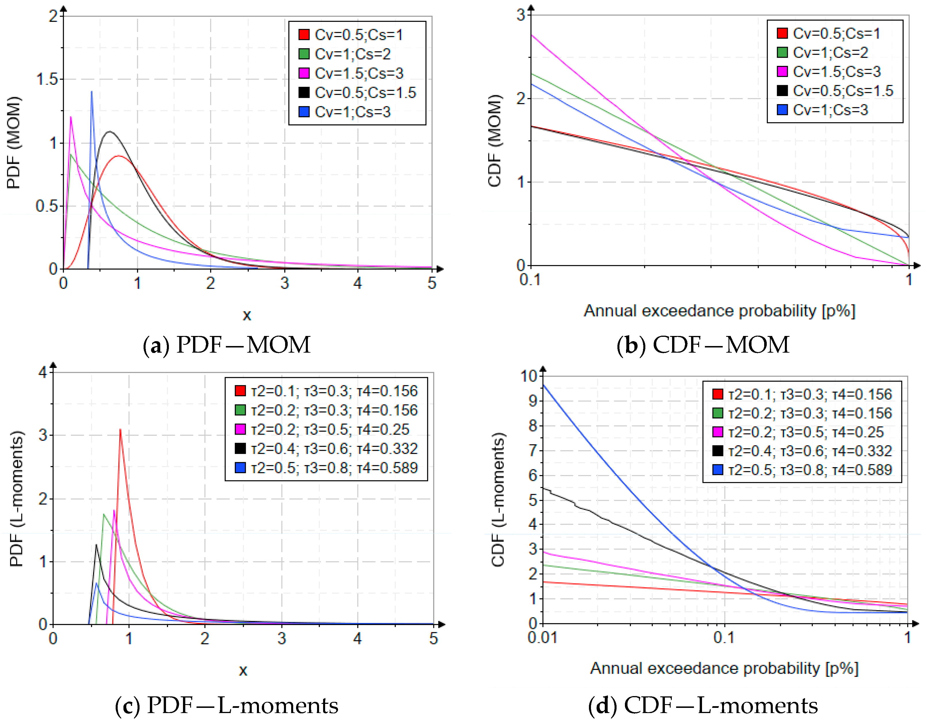
Figure 1. The PDF and CDF for PE3 (MOM and L-moments methods). Where C v , C s , τ 2 , τ 3 , τ 4 are defined in the List of Abbreviations.
Water 17 01539 g001
Figure 2. Evolution graphs of the shape parameter for estimation with MOM, L-moments, and LH-moments (of order 1).
Water 17 01539 g002
Figure 3. Evolution graphs of the parameters for MOM (Romanian methodology).
Water 17 01539 g003
Figure 4. The graph of the relative errors in the estimation of the parameter depending on L-skewness.
Water 17 01539 g004
Figure 5. The variation diagram of linear skewness and linear kurtosis.
Water 17 01539 g005
Figure 6. The graph of the relative errors in the estimation of the parameter depending on LH-skewness.
Water 17 01539 g006
Figure 7. The variation diagram of LH-skewness and LH-kurtosis.
Water 17 01539 g007
Figure 8. The flow chart diagram of the presented analysis.
Water 17 01539 g008
Figure 9. Location of the four analyzed rivers.
Water 17 01539 g009
Figure 10. Maximum annual flows for the Ialomita, Siret, Jijia, and Nicolina Rivers.
Water 17 01539 g010
Figure 11. Box-plot representation of observed data.
Water 17 01539 g011
Figure 12. Evaluations of the quantile function for the five methods of parameter estimation.
Water 17 01539 g012
Table 1. New elements and information presented in the manuscript.
Nr. Crt.New Elements
1New relationships for estimating the shape parameter for the L-moments method.
2New relationships for estimating the shape parameter for the LH-moments method.
3The flexibility of the density function, using the L-moments approach.
4Variation graphs of the shape, scale, and position parameters for a wide range of values of the coefficient of variation and skewness.
5New relationships for estimating the frequency factor for the MOM (including widening the range of annual exceedance probabilities).
6New relationships for estimating the frequency factor for the L-moments method (including widening the range of annual exceedance probabilities).
7New relationships for estimating the frequency factor for the LH-moments method (including widening the range of annual exceedance probabilities).
8The Pearson III distribution’s theoretical biases, both for parameters and quantiles, for an extended field of statistical indicators particular to the L-moments and MOM approaches.
9A comparative analysis to determine the optimal empirical probability for both the distribution and the parameter estimation method.
10Rigorous recommendations regarding the applicability of this distribution.
Table 2. Parameters estimated with MOM and L-moments. Theoretical values.
Statistical indicators—MOM
Parameters C v = 0.5 ; C s = 1 C v = 1 ; C s = 2 C v = 1.5 ; C s = 3 C v = 0.5 ; C s = 1.5 C v = 1 ; C s = 3
α 410.4441.7780.444
β 0.2512.250.381.5
γ 0000.3330.333
Statistical indicators—L-moments
Parameters τ 2 = 0.1 ; τ 3 = 0.3 τ 2 = 0.2 ; τ 3 = 0.3 τ 2 = 0.2 ; τ 3 = 0.5 τ 2 = 0.4 ; τ 3 = 0.6 τ 2 = 0.5 ; τ 3 = 0.8
α 1.2331.2330.4220.2660.093
β 0.1760.3520.7081.9986.013
γ 0.7830.5650.7010.4680.438
Table 3. Biases (%) obtained with MOM ( 2 C v ).
Record LengthParameters C v C s μ Quantiles
0.01%0.10%0.50%1%
1000 α 40.5113.9783.2662.7442.511
β 0.25
γ 0
80 α 4.8960.4970.9040.9993.853.1822.692.469
β 0.225
γ −0.101
50 α 5.2720.4960.8710.9983.8043.1512.672.454
β 0.216
γ −0.14
25 α 6.1420.4940.8070.9963.7123.092.632.421
β 0.199
γ −0.224
Table 4. Biases (%) obtained with MOM ( 3 C v ).
Record LengthParameters C v C s μ Quantiles
0.01%0.10%0.50%1%
1000 α 1.7780.51.514.5463.6172.9552.665
β 0.375
γ 0.333
80 α 2.2290.4951.340.9984.3243.4752.8652.597
β 0.331
γ 0.26
50 α 2.4080.4931.2890.9974.2493.4262.8342.573
β 0.317
γ 0.234
25 α 2.810.4891.1930.9944.1033.332.7712.523
β 0.29
γ 0.18
Table 5. Biases (%) obtained with MOM ( 4 C v ).
Record LengthParameters C v C s μ Quantiles
0.01%0.1%0.5%1%
1000 α 10.5215.1053.9543.1492.803
β 0.5
γ 0.5
80 α 1.2950.4921.7570.9984.7633.7393.0172.704
β 0.431
γ 0.439
50 α 1.4060.4891.6870.9974.6543.6692.9732.67
β 0.411
γ 0.419
25 α 1.650.4811.5570.9934.4463.5332.8842.601
β 0.372
γ 0.379
Table 6. Biases (%) obtained with L-moments ( τ 3 = 0.1 ).
Record LengthParameters L 1 τ 2 τ 3 τ 4 Quantiles
0.01%0.10%0.50%1%
1000 α 10.7110.1820.10.1262.5642.2241.9691.852
β 0.094
γ −0.009
80 α 10.6910.1730.100090.1292.5752.2331.9761.858
β 0.095
γ −0.016
50 α 10.680.9990.1740.100140.1312.5822.2381.981.861
β 0.095
γ −0.02
25 α 10.650.9980.1760.100270.1342.5982.2511.9891.869
β 0.097
γ −0.03
Table 7. Biases (%) obtained with L-moments ( τ 3 = 0.5 ).
Record LengthParameters L 1 τ 2 τ 3 τ 4 Quantiles
0.01%0.1%0.5%1%
1000 α 0.42210.670.50.2517.2112.178.7327.29
β 2.373
γ −0.001
80 α 0.4100.9910.6750.505230.25417.3812.278.7867.325
β 2.411
γ −0.002
50 α 0.4100.9850.6780.508270.25717.4812.328.8177.346
β 2.433
γ −0.002
25 α 0.390.9710.6870.51610.26317.7412.488.8987.399
β 2.492
γ −0.004
Table 8. Biases (%) obtained with L-moments ( τ 3 = 0.9 ).
Record LengthParameters L 1 τ 2 τ 3 τ 4 Quantiles
0.01%0.1%0.5%1%
1000 α 0.04110.9490.90.77310963.0834.3623.52
β 24.6
γ −0.001
80 α 0.040.920.9560.912460.799112.964.1833.9922.74
β 26.373
γ −0.00131
50 α 0.030.8770.960.919450.814115.765.0333.8122.27
β 27.452
γ −0.0013
25 α 0.020.7710.9690.936530.85124.767.7933.2820.87
β 31.299
γ −0.00137
Table 9. The biases (%) for MOM and Q0.01%.
Multiplication
Coefficient, ξ
Coefficient of Variation, C v
0.10.30.50.70.91.11.31.51.72
Record length, n = 80
20.31.73.24.96.68.310121416
30.42.54.97.5101316192125
40.63.46.710141821252833
Record length, n = 50
20.52.34.46.58.71113151821
30.63.46.59.8131720232631
40.94.58.814182327313541
Record length, n = 25
20.73.66.79.8131619222529
31.05.29.714192428333742
41.46.81319263137424754
Table 10. The biases (%) for L-moments and Q0.01%.
L-Skewness,
τ 3
Coefficient of L-Variation, τ 2
0.10.30.50.70.9
Record length, n = 80
0−0.38−0.58−0.65−0.68−0.70
0.2−0.44−0.63−0.68−0.71−0.73
0.4−0.65−0.85−0.90−0.93−0.94
0.6−0.99−1.18−1.23−1.25−1.26
0.8−1.85−2.04−2.08−2.10−2.11
0.9−3.53−3.73−3.77−3.79−3.80
Record length, n = 50
0−0.505−0.773−0.865−0.911−0.939
0.2−0.582−0.836−0.916−0.955−0.978
0.4−0.879−1.14−1.212−1.246−1.265
0.6−1.352−1.612−1.677−1.706−1.723
0.8−2.583−2.846−2.906−2.932−2.947
0.9−5.057−5.344−5.406−5.433−5.448
Record length, n = 25
0−1.283−1.964−2.198−2.316−2.387
0.2−1.465−2.105−2.306−2.405−2.463
0.4−2.261−2.9−3.116−3.203−3.253
0.6−3.751−4.475−4.655−4.736−4.783
0.8−8.018−8.837−9.021−9.102−9.148
0.9−18.09−19.119−19.339−19.435−19.489
Table 11. The morphometric elements for the analyzed rivers [50].
RiverLength
[km]
Average
Stream Slope [‰]
Sinuosity
Coefficient [−]
Average
Altitude, [m]
Catchments
Area, [km2]
Ialomita4171.51.8832710,350
Siret5591.71.8651542,890
Jijia2751.01.451525757
Nicolina20161.37138177
Table 12. The statistical indicators for the analyzed rivers: MOM.
RiverNumber of Records
(n)
Hydrometric
Station
MOM
ξ μ C v C s
[−][m3/s][−][−]
Ialomita33Tandarei22240.5270.33
Siret39Lungoci214430.6341.41
Jijia35Vladeni356.10.8241.85
Nicolina39Iasi314.11.1932.80
Table 13. The statistical indicators for the analyzed rivers: L- and LH-moments method.
RiverL-Moments MethodLH-Moments Method
L 1 L 2 L 3 L 4 τ 2 τ 3 τ 4 L H 1 L H 2 L H 3 L H 4 τ H 2 τ H 3 τ H 4
[m3/s][m3/s][m3/s][m3/s][−][−][−][m3/s][m3/s][m3/s][m3/s][−][−][−]
Ialomita22468.66.131.690.3060.0890.02529356.15.222.300.1910.0930.041
Siret144349011290.60.3390.2280.185193245113589.90.2330.2990.199
Jijia56.123.27.866.010.4140.3380.25979.423.39.256.130.2940.3960.263
Nicolina14.17.553.602.220.5360.4770.29421.68.363.882.340.3860.4640.280
Notes: where L 1 ,   L 2 ,   L 3 , and L 4 represents the first four L-moments; L H 1 ,   L H 2 ,   L H 3 , and L H 4 represents the first four LH-moments.
Disclaimer/Publisher’s Note: The statements, opinions and data contained in all publications are solely those of the individual author(s) and contributor(s) and not of MDPI and/or the editor(s). MDPI and/or the editor(s) disclaim responsibility for any injury to people or property resulting from any ideas, methods, instructions or products referred to in the content.