Article

A Machine Learning Approach for the Estimation of Total Dissolved Solids Concentration in Lake Mead Using Electrical Conductivity and Temperature

Department of Civil and Environmental Engineering and Construction, University of Nevada Las Vegas, Las Vegas, NV 89154, USA
*
Author to whom correspondence should be addressed.
Water 2023, 15(13), 2439; https://doi.org/10.3390/w15132439
Submission received: 26 April 2023 / Revised: 26 May 2023 / Accepted: 28 June 2023 / Published: 2 July 2023
(This article belongs to the Section Water Quality and Contamination)

Abstract

:
Total dissolved solids (TDS) concentration determination in water bodies is sophisticated, time-consuming, and involves expensive field sampling and laboratory processes. TDS concentration has, however, been linked to electrical conductivity (EC) and temperature. Compared to monitoring TDS concentrations, monitoring EC and temperature is simpler, inexpensive, and takes less time. This study, therefore, applied several machine learning (ML) approaches to estimate TDS concentration in Lake Mead using EC and temperature data. Standalone models including the support vector machine (SVM), linear regressors (LR), K-nearest neighbor model (KNN), the artificial neural network (ANN), and ensemble models such as bagging, gradient boosting machine (GBM), extreme gradient boosting (XGBoost), random forest (RF), and extra trees (ET) models were used in this study. The models’ performance were evaluated using several performance metrics aimed at providing a holistic assessment of each model. Metrics used include the coefficient of determination (R2), mean absolute error (MAE), percent mean absolute relative error (PMARE), root mean square error (RMSE), the scatter index (SI), Nash–Sutcliffe model efficiency (NSE) coefficient, and percent bias (PBIAS). Results obtained showed varying model performance at the training, testing, and external validation stage of the models, with obtained R2 of 0.77–1.00, RMSE of 2.28–37.68 mg/L, an MAE of 0.14–22.67 mg/L, a PMARE of 0.02–3.42%, SI of 0.00–0.06, NSE of 0.77–1.00, and a PBIAS of 0.30–0.97 across all models for the three datasets. We utilized performance rankings to assess the model performance and found the LR to be the best-performing model on the external validation datasets among all the models (R2 of 0.82 and RMSE of 33.09 mg/L), possibly due to the established existence of a relationship between TDS and EC, although this may not always be linear. Similarly, we found the XGBoost to be the best-performing ensemble model based on the external validation with R2 of 0.81 and RMSE of 34.19 mg/L. Assessing the overall performance of the models across all the datasets, however, revealed GBM to produce a superior performance based on the ranks, possibly due to its ability to reduce overfitting and improve generalizations. The findings from this study could be employed in assisting water resources managers and stakeholders in effective monitoring and management of water resources to ensure their sustainability.

1. Introduction

Lake Mead, which lies on the Colorado River, is the largest reservoir in the Mohave Desert, Arizona–Nevada region in the Colorado River Basin (CRB) [1,2,3]. The lake is a crucial source of water for more than 25 million people in the southwestern US. The lake is, however, under intense water stress due to the prolonged drought fueled by climate change and the effects of rapid population growth [4,5]. The lake is also faced with water quality impairment caused by elevated levels of water quality parameters (WQPs) such as total dissolved solids (TDS) by natural and anthropogenic activities associated with population growth and urbanization including, but not limited to, irrigation, industrial, and municipal practices [6,7]. Some of these anthropogenic are unintended consequences that need to be minimized [8]. TDS-related economic damages to the CRB are estimated to be over USD 300 million per year, destroying millions of acres of irrigated lands [2,3,9,10,11,12].
TDS is a known physical WQP [3,13,14], categorized by the United States Environmental Protection Agency (US EPA) in its secondary drinking water regulations (SDWRs) with an allowable limit in drinking water set to 500 mg/L [3,12,15]. These SDWRs are described as nonenforceable federal guidelines that cause cosmetic and aesthetic effects. Cosmetic effects include skin or tooth discoloration while aesthetic includes tastes, color [15,16,17]. High levels of TDS in the water can cause scaling and corrosion of cooling systems and boilers. TDS levels in the water are influenced by natural sources, urban runoff, industrial and municipal waste, and chemicals used in water treatment [18]. Other sources of TDS in water bodies include mineral dissolution, desorption of ions, sediments, atmospheric precipitation, chemical, and biological occurrences, and processes including pH, organic carbon, temperature, and rock decomposition [19].
TDS concentration greater than 1200 mg/L is said to be inappropriate for consumption [20]. An increase in TDS or salt loadings in lakes may also contribute to the shifting timing of spring mixings and stratification of lakes. An elevated amount of TDS concentration can cause instability in water columns because of the density difference between less dense fresh and denser saline water. Lake salinization is a major threat to an ecologically significant spring turnover event of water columns as it has the potential to impact its stratification and mixing since the density of the lake profile is influenced by the mixing dynamics of the lake. The buildup of salts in lakes may result in an increment in density gradients in the column of water which could delay, diminish, and/or disrupt the lake from mixing. The effect of temperature on the density of the lake, therefore, largely influences its stratification [21]. An increase in water temperature can vary the biochemical rates of reaction of organisms, bringing about thermal stratification and reduction in lake mixing [14,22].
Researchers in [21] assessed the impact of salinization on lake stratification and spring mixing of two Wisconsin lakes, namely, Mendota and Monona, using an analytical approach to quantify salinity thresholds and the long-term impact of winter salt loading on mixing and stratification. The authors established that increased salt loading causes a delay in spring turnover which prolongs summer stratification and subsequently increases water column stability in north-temperate lakes. Lake mixing is also influenced by water density, which is influenced by water salinization solubility [23]. Microorganisms in water bodies including lakes have the potential to decompose TDS, and their activity may cause fluctuations in TDS concentration. Microorganisms may consume TDS during biological processes which may subsequently influence the dissolved ions in the water and, hence, the EC of the water [24]. Microbial earthworm ecofilters (MEEs), which comprise earthworms and constructed wetland systems, have the potential to cause a significant reduction in TDS concentration by up to 99.8% [25]. MEEs have been used to treat urban runoff. The results showed about a 21% reduction in TDS, showing that TDS concentration is likely impacted by the activities of microorganisms [25].
Measurement or determination of TDS can be performed through direct or indirect means. The direct method of determining TDS concentration is carried out through grab sampling which involves the collection of distinct samples at specific periods which are reflective of the conditions of the water at the time of sampling [26]. The samples collected from the field are prepared and filtrated, then a specific volume is oven-dried in the laboratory and residues are weighed to determine TDS [18].
One way to determine TDS indirectly is by summing measured concentrations of various constituents in the filtered water sample or empirically through electrical conductivity (EC). EC is the property of water that enables it to carry electric current due to the presence of charged ions in the water. TDS concentration and EC are both used to describe the salinity level in water bodies. EC is influenced by factors such as temperature, ion strength, and dissolved ion concentrations measured as TDS [27]. TDS is determined by multiplying EC measured micromhos per centimeter (µS/cm) by an empirical factor as depicted in Equation (1).
T D S = k · E C ,
where TDS is measured in mg/L, k the empirical factor is unitless, and EC is measured in µS/cm. The value of k is expected to increase with an increase in ions in water and is influenced by the activities of all ions in the water and their ionic strength [27]. Empirical factors used in TDS determination range from 0.55–0.9. The actual factor used is influenced by the temperature and soluble components of the water. This factor is determined by establishing repeated paired linear regressions of measurements of TDS and specific conductivity for the water system. High factors have been established for saline water, with the lower value used for water systems with considerable hydroxide or free acid [28]. An empirical factor of 0.67 is adopted for natural water systems according to a study by [28]; this, however, is slightly different from the 0.64 value used by [29] in their study on water quality physical and organic chemical indicators estimation and characterization. Water bodies are categorized into four types based on the TDS concentrations, namely, freshwater (type I) having a TDS concentration < 1000 mg/L, and brackish water (type II) having a TDS concentration between 1000 and 10,000 mg/L. Type III are saline waters with a TDS concentration of 10,000–100,000 mg/L, with brine water (type IV) having a TDS concentration > 100,000 mg/L [27].
TDS analysis is necessary and key as it offers a better understanding of the quality of water, particularly the groundwater, and the effect of seawater intrusion compared with EC analysis. Field measurement of WQPs such as TDS is, however, more difficult, cost-intensive, and time-consuming [14,30,31,32] as compared with EC measurement, as more equipment and time are required for its measurement [27]. EC measurement is quite easy and economical and can be carried out in situ using portable water quality checker devices [27]. As a result, many studies estimate TDS using correlation or empirical factors. TDS estimation from EC is based on the underlying assumption that dissolved solids are mainly ionic species of low concentration needed to yield a linear relationship between EC and TDS [33]. The relationship between EC and TDS is, however, not always linear as it depends on the salinity of the water and the contents of the materials in the water [27].
Machine learning (ML) or artificial intelligence (AI) techniques, however, use implicit algorithms to capture both linear and nonlinear relationships compared to empirical regressions [14,34,35,36] to solve intricate problems [37], and can therefore be applied for effective estimation of the TDS from EC and temperature. AI models have been strongly recommended in recent years for the prediction of WQPs and have been applied in the accurate estimation of water quality index (WQI) compared to conventional models [38,39]. ML techniques have received a lot of interest and have demonstrated astounding successes in various applications in recent years. Both standalone or single and ensemble models have been used in several studies, including water quality studies, to solve challenging problems and obtain accurate estimations of environmental phenomena. Ensemble predictive models are the aggregation of predictions from several ML models to create an overall stronger prediction [40,41,42]. Examples of standalone include support vector machines (SVM), artificial neuron networks (ANN), linear regressors (LR), and K-nearest neighbor model (KNN), while ensemble methods include bagging, gradient boosting machines (GBM), extreme gradient boosting (XGBoost), random forest (RF), and extra trees (ET) [37,41,42,43,44].
Several studies have applied standalone and ensemble ML in estimating WQPs. For example, researchers in [34] applied supervised standalone and ensemble ML models and remote sensing in the estimation of chlorophyll-a and suspended solids in water bodies in Brazil and achieved a prediction accuracy of R2 > 80% for both WQPs, which is a demonstration of the effectiveness of ML models. Similarly, researchers in [45] applied remote sensing and AI models evaluate to evaluate different WQPs in the Hudson River in New York and found the multivariate adaptive regression spline (MARS) model to be the best-performing model for monitoring the WQI in the river. Conversely, researchers in [46] found the forward selection M5 model tree (FS-M5 MT) to be the best-performing model for the estimation of WQI classifications for the Karun River in Iran.
Additionally, researchers in [39] utilized ML classifiers (MLC), namely, multivariate adaptive regression spline (MARS) and least-square support vector machine (LS-SVM) for the prediction of chemical oxygen demand (COD) and five-day biochemical oxygen demand (BOD5) indices in the same Karun River, Iran, and compared results to the outputs of ANN, multiple regression equations, and adaptive neuro-fuzzy inference system (ANFIS), and found the results of the MLC to be effective in predicting the WQPs.
Researchers in [47] applied ML to predict suspended sediment load in three river systems in the US, namely, the Missouri, Mississippi, and Rio Grande Rivers, using the ANN model. The results of the ANN model were compared to results from multiple linear regression (MLR) and multiple nonlinear regression (MNLR) models, and they found the ANN to be a better predictor compared to the MLR, showing superior performance, particularly in the rivers with fewer variations, with R2 = 97%, 96%, and 65%, respectively, for the Missouri, Mississippi, and Rio Grande Rivers.
Researchers in [48] utilized ML to assess the spatiotemporal variability of salinity in Lake Urmia in Iran, which is known to be the second-largest hypersaline lake globally. The authors found the ANN to be an accurate estimator of salinity concentration in the lake, with an R2 of 94%, compared to ANFIS and MLR models.
Researchers in [49] also applied ML models including ANN, SVM, and XGBoost in predicting contamination levels of pesticides and nitrates in groundwater to the water quality of 303 wells across 12 midwestern states in the US. Results from these models were compared to baseline LR. The researchers obtained the highest R2 of 69% for pesticide contamination using XGBoost and 53% for nitrate contamination using the ANN model. The LR was the worst-performing model, with R2 of 13% and 11% for both nitrate and pesticide, respectively.
Estimating TDS concentration using EC and temperature and ML techniques is motivated by the past success of ML models in water quality studies and the fact that TDS measurement is crucial for determining water quality, monitoring, and managing aquatic ecosystems. The health of people, aquatic species, and the general ecological balance can all be negatively impacted by high levels of TDS in the water. Therefore, it is important to develop effective and robust algorithms for the accurate estimation of TDS for efficient decision making concerning water quality management and ecosystem protection. Consequently, our study is leveraged on the existence of a relationship between EC and TDS, and the associated effect of water temperature on EC to capture the intricate interactions and nonlinear patterns related to TDS dynamics in Lake Mead using novel and promising ML techniques that provide the ability to understand complex patterns and relationships from big datasets for a robust and accurate estimation of TDS in Lake Mead.
This study, therefore, aims to develop and assess the predictive accuracy of ML models for the estimation or prediction of TDS in Lake Mead using EC and temperature. The developed models can be utilized to produce accurate and cost-effective TDS estimations, which can help with managing and monitoring water quality efforts. To achieve the objective of the study, the following questions were formulated. These are:
  • What is the strength of the relationship between TDS, EC, and temperature in Lake Mead?
  • How does the accuracy of estimation of TDS from EC and temperature using ensemble models compare with a standalone model?
  • Which ML model offers the best predictive accuracy in the estimation of TDS using EC and temperature?

2. Materials and Methods

This section presents the description of the study area, the data used, and the techniques used to achieve the objective of the study.

2.1. Study Area Descriptions

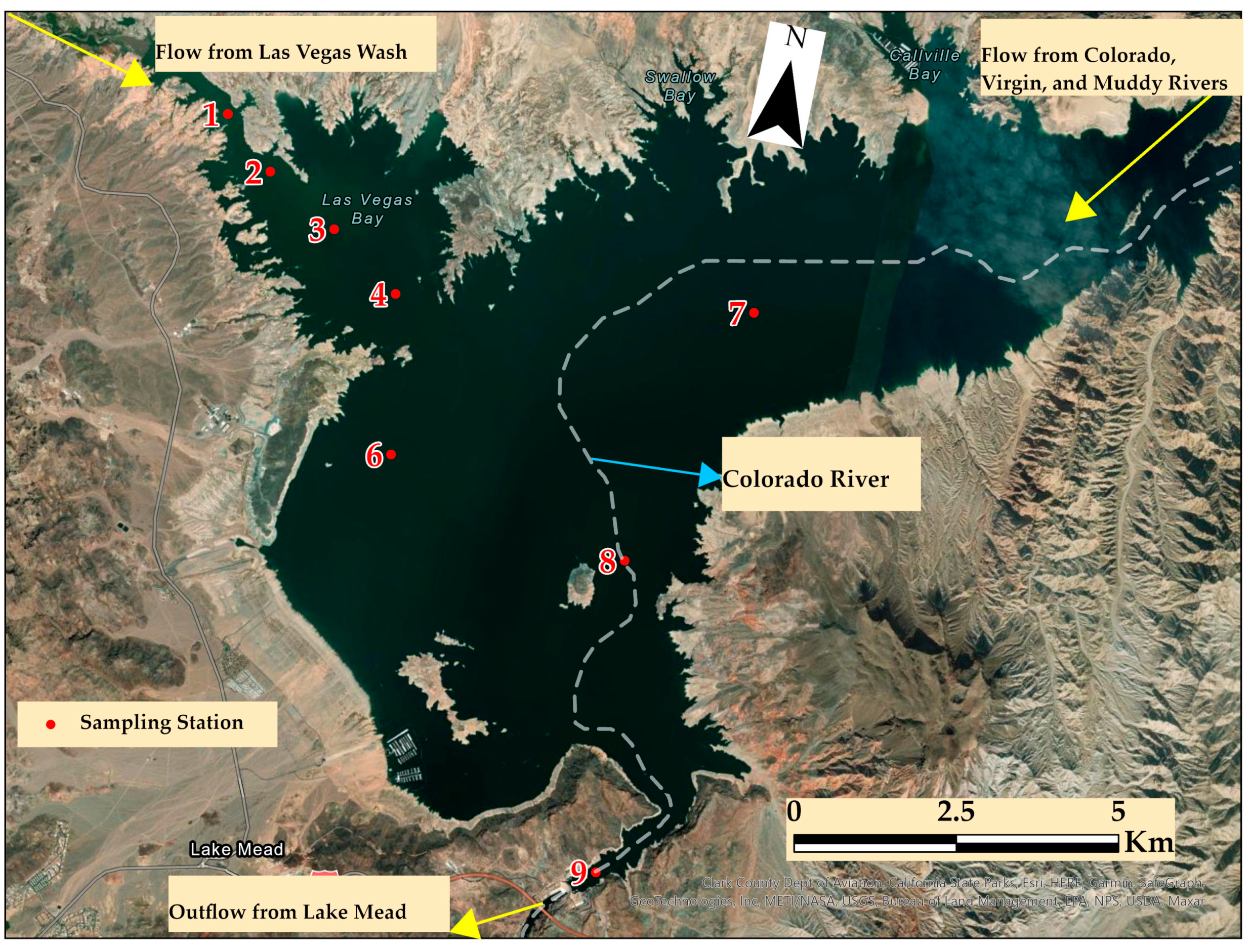
Lake Mead is the study area for this study. The lake lies on the Colorado River and it is the largest reservoir on the approximately 2333 km river located in the Mohave Desert, Arizona–Nevada region [1,2]. Lake Mead was formed after Hoover Dam was constructed in the 1930s and it is the largest reservoir in terms of water capacity within the United States. It is the source of water for about 90% of the Las Vegas Valley water supply [50,51]. Lake Mead is one of the water bodies currently under intense water stress due to climate change and the effects of rapid population growth. TDS is one of the known water parameters affecting the quality of water in Lake Mead, which is the source of water for more than 25 million people in the southwestern US, including Nevada. The average yearly precipitation for the lake is 14.58 cm [52]. TDS loadings into the lake are from the mainstem Colorado River, Little Colorado River, Virgin, Muddy Rivers, and the Las Vegas Wash [53]. The natural TDS of Lake Mead is about 610 mg/L which is above the EPA-recommended 500 mg/L. As a result, many commercial facilities and residents in the Las Vegas Valley (LVV) use ion-exchange-based water softeners that contain sodium or potassium chloride brines to remove TDS from their drinking water. The regenerant salt produced from the ion exchange process is discharged into sewer lines; it may not be removed during wastewater treatment and is subsequently discharged into Lake Mead [54]. The LVV has seen a great increase in population over the last three decades, causing an increase in commercial, residential, and industrial discharges. The use of salt and water softeners by households and in commercial quantities continues to increase. As the population in the LVV continues to grow, and with the current trend of drought in the Colorado River, TDS concentration release into Lake Mead may be expected to continue to rise over time [6], making TDS a WQP of concern in this study. Furthermore, a study by [6] to assess the TDS contribution to the Colorado River associated with the population growth in the LVV using system dynamic models revealed that the TDS concentration in the Las Vegas Wash (LVW) will rise to about 14% in the year 2035 and a 10% population increase with water softeners reduction will also reduce the TDS concentration by 126 mg/L. A detailed map of the study area presenting the sampling site on Lake Mead used in this research is presented in Figure 1.

2.2. Data Collection

Data used for this study were obtained from the city of Las Vegas, NV, USA. The LVW and Lake Mead are sampled annually for water quality data, including TDS, EC, and temperature, by the cities of Las Vegas, North Las Vegas, Clark County Water Reclamation District, and Henderson. The purpose of these monitoring activities is to comply with the Nevada Division of Environmental Protection’s (NDEP’s) yearly National Pollutant Discharge Elimination System (NPDES) permits (NDEP). Data used in the monitoring operations are gathered into a master database, maintained by the City of Las Vegas. Table 1 below provides a summary of the Lake Mead sampling sites and frequency as described in the Lake Mead and Las Vegas 2019 Annual Report [55]. The approximate locations of the stations are further presented in Figure 2 [55]. While temperature and EC measurements were made using a YSI EXO data sonde, TDS concentration was measured in the laboratory at the Clark County Wastewater facility, NV, USA, utilizing gravimetric (physical filtering) and drying procedures. The frequency and station of measurement were selected based on background information, location, and relevance.

2.3. Modeling and Analysis

Modeling and analysis were carried out using several ML models. These models are categorized as standalone and ensemble models. Standalone models used in the study include LR, SVM, ANN, and KNN, and ensemble models include bagging, GBM, XGBoost, RF, and ET [34,37,49,56,57].
The single models allow for fundamental modeling strategies as they serve as basic blocks for providing insights into the specific and individual performance of different techniques. They are therefore used as a baseline for comparison with more complex and sophisticated models. Ensemble models, on the other hand, combine multiple single models to build a more reliable and sophisticated model which captures a greater variety of patterns and minimizes the impact of individual model biases. Our study, therefore, seeks to leverage the potential advantage of integrating single models for powerful estimation [37,41,43,44]. We use both standalone and ensemble models in the study to address a variety of needs so that researchers and stakeholders who prefer the standalone models can learn and benefit from the performance and the constraints of these models, while those exploring beyond the predictive accuracy of standalone models could do so with the ensemble techniques, which can improve the generalization compared to standalone models [37,58].
We deliberately applied a variety of standalone and ensemble MLs aimed at exploring the effectiveness and applicability of the various ML algorithms for estimating the concentration of TDS using EC and temperature. The use of several models was necessary to compare and assess the efficacy of these models in capturing the intricate interactions between the EC and temperature and TDS concentrations. TDS concentration in the water is affected by several factors, making its quantification complex, hence the need to explore several ML algorithms. Additionally, each of these models has its unique advantages, underlying presumptions, and limitations. To give a thorough analysis that considers numerous algorithmic techniques and their corresponding evaluation metrics, we made use of a wide range of models. This enabled us to discover the models that are most robust and effective in capturing the underlying patterns in the TDS data, which is necessary to gain a more thorough and comprehensive knowledge of the applicability of the models in TDS estimations, thereby contributing to the scientific rigorousness of our research [34,49,56,57].
The models used in this study are described in detail in the subsequent subsections.

2.3.1. Standalone ML Techniques

A description of the various standalone ML techniques used in this study is presented in the following paragraphs.
LR is the most common algorithm that measures the relationship between variables used for prediction. It assumes that there is a linear association between the input features and the response variable. It works by estimating the coefficients of each of the input features to reduce the associated sum of squared errors. They are simple but powerful models used for decision making. The main hyperparameters of LR are the regularization parameter, denoted as α, which regulates the trade-off between complexity and overfitting of the model. Regularization, also termed shrinkage, is utilized to obtain reliable predictor coefficients when the predictors are strongly correlated. They work by imposing different penalties through “ridge” or “least absolute shrinkage and selection operator (LASSO)” mechanisms. The ridge maintains all the predictors in the final model by applying various penalties, whereas LASSO ensures the sparsity of the findings by precisely shrinking coefficients with less significant features to zero [59]. The extent of the regularization and the sensitivity of the model to outliers can be controlled via hyperparameter adjustment.
We used ordinary least square regression (OLS) which minimizes the sum of square errors between the observed and simulated values without any applying penalty on the coefficient [60,61]. Linear regression models are classified as simple or multiple regressions [60,62,63]. A simple regression analysis relates a single independent or predictor variable to a single dependent or response variable. The multiple regressions contain multiple predictors to predict the response variable. The MLR test allows for the combination of multiple predictors to explain the response variable [43,63]. Our study utilized the MLR using the EC and temperature as predictors for predicting TDS.
SVM: This technique was first created for classification purposes in the early 1990s and was later extended for regression [41,64,65]. It is a supervised ML technique utilized for classification based on statistical learning theory using hyperplane fitting which is said to provide the best separation between two classes in a multidimensional feature space. SVM attempts to minimize the difference between the measured and predicted data. Training of SVM is performed with learning algorithms that are derived from optimization theory. The main hyperparameters for the SVM include the kernel type, kernel-specific parameters such as the degree (°) and kernel width (γ), and the regularization parameter “C” [59]. The SVM uses different kernels including the linear, radial function, sigmoid, and polynomial. The linear kernel requires less computing power. The nonlinear kernels have the advantage of nonlinear forecasting although they cause the features to be projected to a higher-dimensional space, obscuring their original attributes; hence, ranking the features by importance is meaningless [44,49]. The radial kernel is, however, found to pose less numerical complexity [44]. The kernel type enlarges the feature space and generates nonlinear boundaries while C is a regularization parameter that controls the trade-off between minimizing the training error and then maximizing the margin. A high C value results in low biases and large variance, and vice versa. The γ, on the other hand, is a representation of kernel width that influences the class-dividing smoothing for the hyperplane shape. High γ value results in high biases and low variance, and vice versa. The ° hyperparameter is used in constructing separate hyperplanes when using the polynomial kernel. SVM has been found to outperform other ML algorithms, including neural-network models, in past studies [49,59,64,66,67].
The KNN is a nonparametric ML model used for classification and regression predictions and is used to identify the k-training samples in the training set that is closest to the target. Hyperparameters in the KNN model include the number of neighbors depicted by k, which establishes the locality and generality of the model. Another known hyperparameter for the KNN is the distance metric, which evaluates the similarity and other required preliminary processing steps. Distance metrics such as Euclidean and Manhattan distance are often used. Based on the closest distance, the most related K value is chosen to categorize the input features. The KNN algorithms rely on the voting function of the chosen ideal k value and distance [40,42,58,68,69]. The KNN techniques have been employed in various studies with a significant level of accuracy, including one where short-term energy forecasted was performed with a mean absolute percentage error (MAPE) of 4% [68] and the estimation of chlorophyll-a and suspended solids concentration in water bodies in Brazil with R2 > 80%.
The ANN models are flexible computational models inspired by the makeup and biological neurons of the human brain [49,56]. They are mathematical equation networks made of an input and one or several hidden layers consisting of interconnected nodes called neurons and an output layer [70]. ANN neurons are imitated to perform a nonlinear transformation to yield output. ANN models have the potential to predict outputs based on training and learning computational procedures. The hyperparameters to improve the performance of the ANN include the number of iterations, hidden layers, number of epochs, and neurons, learning rate, and transfer functions. Multilayer perception (MLP), an advanced representation of ANN, and a large iteration were utilized to improve the performance of the model [47,49,65,71,72,73].

2.3.2. Ensemble ML Techniques

Ensemble ML models consist of several base learners which are trained and aggregated to analyze and address various real-world problems [57]. The authors of [41] utilized an ensemble or ML predictive model and produced greater predictivity compared with standalone models such as the SVM. This study aimed to compare predictive water quality results from standalone ML techniques to ensemble ML. The ensemble ML techniques used in the study are described in the paragraphs below.
Bagging technique: This technique is also known as bootstrap aggregating. It is one of the earliest and simplest, yet most effective, ensemble ML techniques. It calculates its final predictions by averaging the results from all decision trees built on bootstrapped training subsets [59,74]. In this ensemble method, the bootstrap sampling procedure is used to acquire random subsets of the training set of the original model with replacement. It is used in regression and classification to improve the precision of the ML approaches by aiding in the deduction of variance and the enhancement of the robustness of the model using decision trees. Hyperparameters in the bagging techniques are mainly the choice of the base models such as decision trees and the number of base models used [57,59,75].
GBM technique: This technique creates prediction models by utilizing an ensemble of weak classifiers such as decision trees [57]. Hyperparameters for the GBM include the number of iterations, the learning rate, the loss function, and the maximum depth of the single weak models. The boosting model consists of several logistic regression or decision trees built by relying on some randomly chosen trees, with its performance improved by iteratively adding new randomly chosen decision trees which help to improve the accuracy of the previous iteration model [57,68,76].
Extra trees (ET) technique: Extremely randomized trees is another name for this ensemble method. The extra trees are an ensemble of regression trees or unpruned decisions using classical top-down approaches. Their primary distinction from other tree-based methods such as random forest—and what makes them unique—is how they divide nodes. They randomly choose cut points to divide their nodes, and they develop the trees using the entire learning sample. In this method, the bootstrap sampling approach is not used, and all trees are trained using the entire training dataset. Hyperparameters in the ET models include the number of trees, the number of features for splitting at each node, and the maximum depth of the trees [57,68,77].
RF: This technique combines the performance of several decision trees or individual learners to predict the value of a response variable. Each of the decision tree predictors uses randomly selected bootstrap sets from the original training set with replacement [58,65,78]. It receives input (in this case, water quality parameters) and performs analyses for the training data by building several regression trees. The results of these analyses are then averaged in the RF analysis. Hyperparameters for the RF include the number of trees, features to consider at each split, the maximum depth of trees, and the minimum number needed for node splitting. RF increases the diversity of its trees by ensuring that the trees grow from different training data subsets to avoid the correlation of different trees [65,65,78,79].
XGBoost: This technique uses weak learner decision trees in a sequence in which the next tree learning comes from the errors of the previous tree to produce highly accurate predictions [41]. The algorithm was developed in 2016 at the University of Washington. XGBoost shares many characteristics and advantages with RF forest in terms of predictive performance, simplicity, and interpretability. The key difference between the two is the fact that decision trees are built sequentially in XGBoost rather than them being built independently [80]. Hyperparameters control the structure of decision trees in the XGBoost, including the maximum tree depth, which regulates the overfitting, and ϒ, which is a regularization parameter (a larger value of ϒ leads to an enhanced conservative model). Other hyperparameters of the XGBoost include learning rate, number of estimators, and iterations [49]. The XGBoost was applied on the EC and temperature as a predictor to establish a predictive model for the TDS.

2.3.3. ML Model Hyperparameter Optimization

We first set aside the dataset for the whole of 2021 capturing a wide range of spatiotemporal information to be used as an unseen dataset for external validation to assess the models’ performance in a real-life scenario where newly acquired and unknown datasets are encountered. This is necessary and is often used to offer an unbiased assessment of the models’ performance and to validate their potential for generalization [40,59,64,66,74,81]. The rest of the dataset (2016–2020) to be used for the ML modeling was randomly split into 80%/20% proportions, respectively, for training and the test sets. We used the 80% for the training and development of the model and consequently used the 20% test sets for the model evaluation [37,42,82]. The length of the training dataset is generally larger than the testing data because the training stage of modeling seeks to identify the optimal hyperparameters to achieve the best generalization [64].
The predictive potential of ML is heavily dependent on the values of the hyperparameters that regulate the model’s learning process, hence it is expedient to explore which combinations of hyperparameters generate an optimal model [42]. We performed a grid search, which is a computation-intensive fine-tuning technique to optimize the hyperparameters and works by performing a thorough search to find the optimum values of hyperparameters, taking into account all conceivable combinations [37,42,82].
We utilized the k-fold cross-validation mechanisms to overcome the intrinsic deficiencies and issues of overfitting in the model. The k-fold cross-validation is a splitting process that allows for the repetition of the training process to improve the robustness of the ML algorithm. It works by following these numerical steps: (i) Allocating observed sample points into k mutually exclusive and collectively exhaustive folds in an even manner without shuffling by defaults; (ii) Using the k-1 part of the folds for training the model and the remaining one part for the model validation; (iii) Steps (ii) are then repeated till each part is used to train and validate; (iv) Average performance of k estimations is then computed as the model performance [37,42,82,83,84]. The k-fold cross-validation is said to provide a more consistent outcome and reduce biases and overfitting-related problems [34,85]. This study, therefore, combined the grid search with fivefold cross-validation, i.e., k = 5, for the hyperparameter optimization.
Many studies utilize 10 folds to find a balance between computing efficiency and offering an unbiased and robust model performance [34,37,42,82,85,86,87], but our study applied five folds due to the data size and also to reduce the associated computation time and biases in a less-computation-intensive manner. Using grid search with 10 folds could take significant time, up to several days, owing to the several models being analyzed. Many studies have also utilized several other folds, including the five folds in the hyper-tuning processes [88,89,90,91,92]. Researchers in [91] described the usage of the fivefold as successful in the prediction of WQI in a cost-effective and timely manner. Data science resources such as [93] provide a repository of base ML algorithms for analysis.
Analyses were carried out on a computer system which has the following specifications: Intel(R) Core (TM) i3-4150 CPU @ 3.50 GHz, RAM 16.0 GB, Windows 10 Pro, 64-bit operating system, x64-based processor. All the ML techniques were carried out using mainly Python version 3.9.12 employing libraries such as NumPy version 1.21.5, Pandas version 1.4.2, Seaborn version 0.11.2, and Matplotlib version 3.5.1, which are used for the analysis and visualization of datasets [94]. Python scripts were created and executed in the Jupyter Notebook environment which is a web-based graphical interface used for executing Python statements [94]. Python is free, relatively simple, and has a lot of useful data-science-related libraries [95].

2.3.4. Model Evaluation Metrics

To evaluate the model performance in estimating the observed data, widely used statistical metrics such as the coefficient of determination (R2), mean absolute error (MAE), percent mean absolute relative error (PMARE), and root mean square error were utilized [96,97,98]. These evaluation metrics were carried out using Python programming language in the Jupyter Notebook environment. R2 values indicate the proportion of variance in the dependent variable (TDS) which is predictable by the independent variable (EC and temperature). Values range from −∞ to 1, with 1 being the best value [99]. Additionally, we utilized the scatter index (SI), which is a representation of RMSE difference to the mean of the observed values, the Nash–Sutcliffe model efficiency (NSE) coefficient, which is a measure of the relative magnitude of the residual variance to the measured data, and percent bias (PBIAS), which is the probability of the predicted outcome to be greater or less than the observed value [45,97,98,100,101]. Lower values of RMSE, MAE, PMARE, and SI are an indication of better performance of the model, with zero indicating a perfect score [32,66,69,97,98,100,101,102]. NSE values range from −∞ to 1, with values of about 0.75 to 1.00 said to be very good and values less than 0.4 being unsatisfactory. Lower PBIAS values are an indication of accurate prediction. Positive and negative PBIAS represents underestimation and overestimation in the precision, respectively [97,98,103]. Equations for the model evaluation metrics are presented in Equations (2)–(8) [32,66,69,97,98,100,101,102].
R 2 = 1 i = 1 n Y p r e d Y o b s 2 i = 1 n Y o b s m e a n Y o b s 2
M A E = 1 n i = 1 n | Y o b s Y p r e d |
P M A R E = 1 n i = 1 n | Y o b s | 100
R M S E = 1 n i = 1 n Y o b s Y p r e d 2
S I = 1 n i n ( Y p r e d Y p r e d m e a n ) ( Y o b s Y o b s m e a n ) ² 1 n i n Y o b s
N S E = i = 1 n Y o b s Y p r e d ² i = 1 n Y o b s Y o b s m e a n ²
P B I A S = i = 1 n Y o b s Y p r e d i = 1 n Y o b s × 100 % ,
where Yobs, Ypred, Yobsmean, and Ypred are the observed, modeled, mean of the observed, and mean of the modeled values, respectively.

3. Results and Discussion

This chapter presents the results and discussion of the study which aimed to estimate TDS concentration using EC and temperature data as primary predictors. TDS is a crucial indicator of water quality that affects many aspects of water use, including taste, and suitability for various uses. Effective water resource management, monitoring, and treatment depend on accurate TDS prediction. Due to their ease of measurement and significant association with TDS, temperature and EC have been explored in several studies as proxies for TDS estimations. This research focuses on analyzing several ML models to determine how well they perform in estimating TDS based on temperature and EC data gathered from Lake Mead. The results of this study will advance the understanding of the concept and help people make better decisions on how to maintain water quality.

3.1. Statistical Summary

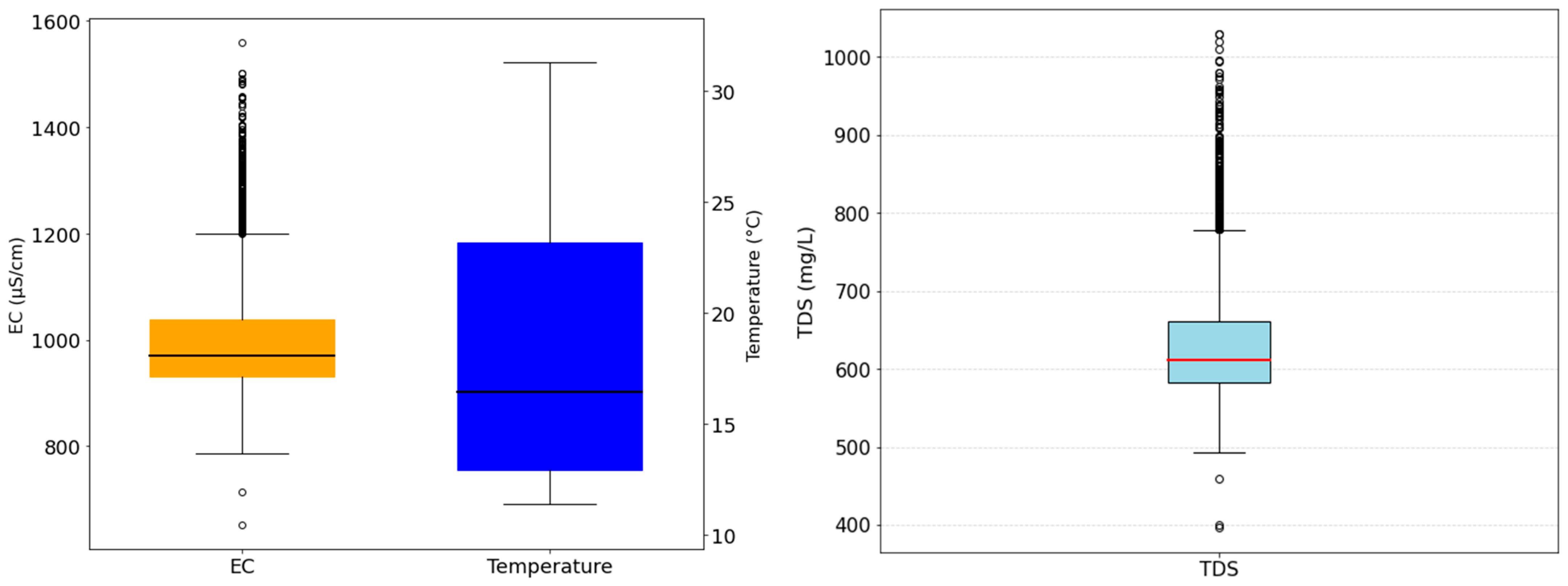
The boxplots showing variations in the EC, temperature, and TDS for all the data collected in the study area are presented in Figure 3. From the plots, it is seen that the highest TDS, EC, and temperature values recorded at the study area are 1030 mg/L, 1559.60 µS/cm, and 31.29 °C, with the lowest values being 397 mg/L, 652.40 µS/cm, and 11.39 °C, respectively. The summary statistics for TDS concentrations for the locations under consideration over an approximate six-year period (2016–2021) are presented in Table 2. Station LWLVB1.2 recorded the highest TDS concentration of 1030 mg/L over the period under study, while station LWLVB3.5 recorded the lowest concentration, at 493 mg/L. The mean and standard deviation of TDS concentration recorded was 598 mg/L and 84 mg/L, respectively. The greatest average TDS concentrations were found at the LVW stations, with values of 716, 670 mg/L, 555 mg/L, and 459 mg/L, as shown in Table 2. From the table, it is seen that the TDS levels varied among the stations. The Las Vegas Wash is a conduit of stormwater and urban overflow from the Las Vegas Valley to Lake Mead, which can impact the lake’s water quality significantly. The LVW watershed drains more than 5000 km2 of nonpoint surface and groundwater discharges from the Las Vegas metropolitan area of about 1165 km2, as well as treated wastewater from the municipal wastewater treatment facilities in the cities of Las Vegas, Henderson, North Las Vegas, and Clark County [52]. The increase in TDS in the LWV may be caused by several of the contaminants drained by the LWV watershed. Compared to the Las Vegas Wash stations, the basin stations had the lowest mean TDS values with less variability; the average values range from 581 mg/L to 598 mg/L for the basin stations. Variability in the TDS concentration could largely be due to factors including, but not limited to, human activities, climate change, and geological formations. The decrease in TDS concentration from the Las Vegas Wash to the Boulder Basin is also influenced by the amount of storage in the basin. The changes in the TDS concentration may also be due to prior events of irrigation, precipitation, runoff, and evaporation, which likely impact the salt concentrations [104]. Salt is left behind after the drying or evaporation process and accumulates in water bodies [104]; this is more prominent in rivers (the wash), unlike the lake (basin) which has large storage.

3.2. Correlation Analysis

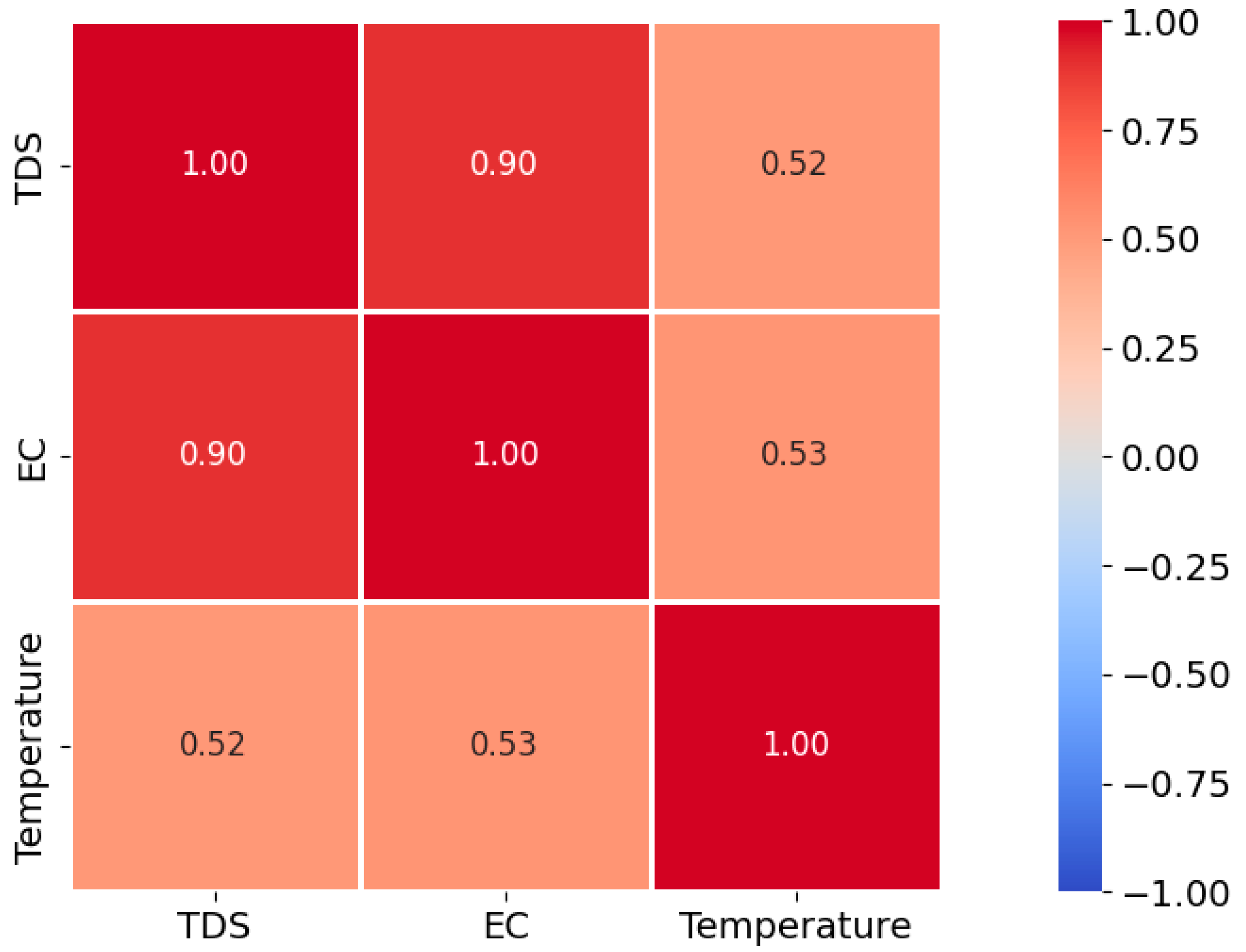
Correlation investigates the strength of relationships between the water quality parameters under study (TDS, EC, and temperature). The correlation coefficient (R) quantifies the strength and direction of the linear relationship between variables. R values range from −1 to 1, with values closer to 1 indicating a stronger correlation. Negative values indicate negative correlations.
The correlation heatmap to measure the degree of association between TDS, EC, and temperature is shown in Figure 4. From the figure, it is seen that TDS and EC have a strong positive correlation, with R = 0.90, demonstrating that a rise in TDS will cause an equal rise in EC. This relationship is expected given that EC measures the electrical conductivity of water, which is influenced by the presence of ions in solution, and TDS measures the concentration of dissolved solids in water. Studies from the past have established a connection between TDS and EC [27,105]. Temperature exhibits a moderately strong association with TDS and EC, with R > 0.50. This association was also anticipated since temperature variations might have an impact on the solubility of specific substances in water, which can alter TDS and EC. Studies have confirmed the existence of salinity (TDS), EC, and temperature [106]. The EC of water is influenced by its temperature as ions move faster when the water temperature is increased [107]. The temperature of the water can also affect the speed of biological and chemical processes, which can have an impact on water quality. When analyzing water quality data and developing monitoring plans, it is, therefore, crucial to take these relationships into account because changes in one could signal changes in other parameters. The correlation matrix can also guide further research by pointing out potential sources of water quality variance.

3.3. ML Predictions and Analysis

3.3.1. ML Model Hyperparameters Optimization

The grid search with fivefold cross-validation as described in Section 2.3.3 was used to find the optimal hyperparameters for each model. The obtained optimal hyperparameters to maximize accuracy [82,108,109] are presented in Table 3.

3.3.2. Model Performance Assessment

The model accuracy assessment was conducted on (i) the training dataset, (ii) the testing dataset, and (iii) external validation (unseen dataset). Carrying out a model assessment on these different datasets aids in fully comprehending the model’s strengths, limitations, and generalization capabilities. Additionally, it enables us to select, optimize, and deploy models in an informed manner, guaranteeing that the model works effectively in real-world scenarios and preventing overfitting or subpar generalization.
The findings of the ML analysis of the water quality data are presented in this chapter, with a particular emphasis on estimating TDS-based EC and water temperature. Several ML models such as RF, SVM, LR, and ensemble models were used to estimate TDS concentration.
The findings on the performance of the ML models are presented in this section.
Results were obtained for the standalone and ensemble ML models. A summary of the performance evaluation of the models is presented in Table 4 for the training, testing, and external validation phases of the model. Generally, evaluation metrics at the training phase of the model do not serve as a great baseline for performance evaluation [110].
Accurate assessment and comparison of the effectiveness of predictions of models is required in making well-informed decisions in a variety of fields. Our findings reveal that the standalone models had R2 of 0.80–0.84 (80–84% variability in TDS being explained by the EC and temperature) across the training, testing, and external validation datasets while the ensemble methods showed R2 of 0.77–1.00 (77–100% variability in TDS being explained by the EC and temperature) across the training, testing, and external validation. In terms of the R2, we see that the ET could explain 100% of the TDS variability in the training set but only explains 80% and 77% in the training and external datasets, which could be due to issues of overfitting and bias–variance trade-offs in the training dataset, hence the need to evaluate the external datasets to offer an unbiased assessment of the models’ performance and to validate their potential for generalization [40,59,64,66,74,81]. All the models exhibit varying performance in the evaluation metrics from the training to the external validation. Models that show exhibit consistent performance across all datasets are more likely to perform effectively in real-world settings. From the analysis, models such as the LR produced R2 of 0.80–0.83, with RMSE of 33.09–34.77 mg/L, and the SVM produced R2 of 0.80–0.83, with RMSE of 34.40–35.5 mg/L (showing little variation), and models such as ET, bagging, and XGBoost, although producing high R2, showed the greatest variability in the three datasets, with R2 ranging from 0.77–1.00 and RMSE from 2.28–37.68 mg/L, questioning their applicability for simulating real-life scenarios.
In comparison, researchers in [111] found that the RF was the best-performing model for estimating TDS, with R2 of 0.79, RMSE of 12.30 mg/L, MARE of 0.082, and NSE of 0.80, although they used remote sensing images as their features, and also conducted their research in a different water body (Lake Tana) located in Ethiopia (no external validation was carried out). Our research produced R2 of 0.80, RMSE of 35.25 mg/L, MARE of 0.0342, and NSE of 0.80 on the external validation for the RF. There is a huge difference between their RMSE and ours, possibly due to the variation in TDS between the two water bodies. While their TDS values ranged from 7.30 to 113.3 mg/L, ours range from 397 to 1030 mg/L. Additionally, researchers [112] found specific conductance to explain 87.6 to 96.9% variation in TDS at 25 °C using multiple linear regressions models for four sites at Yuma area of the Colorado River, located between the Imperial Dam and the southerly international boundary between the USA and Republic of Mexico with TDS ranging from 690 to 2580. Recorded RSME also varies from 5.91 to 26.6 mg/L. Researchers in [110], however, found the Gaussian process regression (GPR) (a nonlinear regression model) to be the best performing for modeling TDS from WQPs obtained from groundwater, surface water, and drinking water, including pH, TSS, turbidity, and EC, among others, with recorded average values of R2, RMSE, and MAE of 98.7%, 7.910, and 4.090, respectively, for a study conducted in Tarkwa (mining community in Ghana). TDS values collected ranged from 8.81 to 534.00 mg/L.
Analyzing the models based on individual indicators can be complicated and may not give a holistic assessment and picture of how well they perform. To overcome this challenge, we created a ranking summary that combines various performance metrics and offers a thorough evaluation of model performance, as presented in Table 5. We provide a ranking summary of the evaluation metrics to offer a structured and consistent overview of the model evaluation across the various datasets. The models are ranked for each dataset according to how well they perform in various measures with the highest R2 and NSE assigned 1 and the lowest assigned 9. Similarly, models with lower values of MAE, RMSE, PMARE, SI, and absolute values of PBIAS are assigned 1, and the models with the highest values of these metrics are assigned 9 [32,66,69,97,98,100,101,102].
From the results, we can observe the performance of the model changing from the training to external validation phases of the datasets, with a drastic change observed from the training stage to another dataset (an example is the case of the LR where the overall ranks changed from 7.1 in the training dataset to 4.3 in the testing dataset and to 2.0 in the external validation, an indication that performance evaluations in the training dataset may not be a great baseline for accurate model prediction, particularly with the close ranks in the testing and external validation dataset [110]).
It is seen from the results that the GBM ensemble method generally performs better than all the models based on the metrics used, with relatively lower ranks across the datasets (average rankings of 3.0, 1.7, and 4.6, respectively, for the training, testing, and external validation datasets and an overall average of 3.1) due to its underlying operations of using complex relationships to iteratively build trees and learn from the errors of preceding weaker trees [109,111]. These results, therefore, demonstrate the reliability and efficiency of the GBM in estimating TDS from EC and temperature. The LR, ANN, and XGBoost, however, showed a superior performance on the external validation datasets with ranks of 2.0, 2.7, and 3.1, respectively. Although the LR model shows relatively weaker performance on the training dataset (ranks of 7.1), which could be due to overfitting [40,49,57,113], its performance on the external validation dataset was most superior, possibly due to the existence of an established relationship between the TDS and EC, although the relationships may not always be linear [27,112].
The analysis based on model evaluation generally presents an understanding of the varied predictive potential of the ML models in different data phases due to several factors, including the complexity of relationships that exist within the data being analyzed [59].
The results from the evaluation metrics implied that ML models could be effectively used to accurately predict TDS in a very cost-effective manner, which is helpful for the water quality monitoring and aids in making well-informed decisions for water quality treatment and allocation of resources.
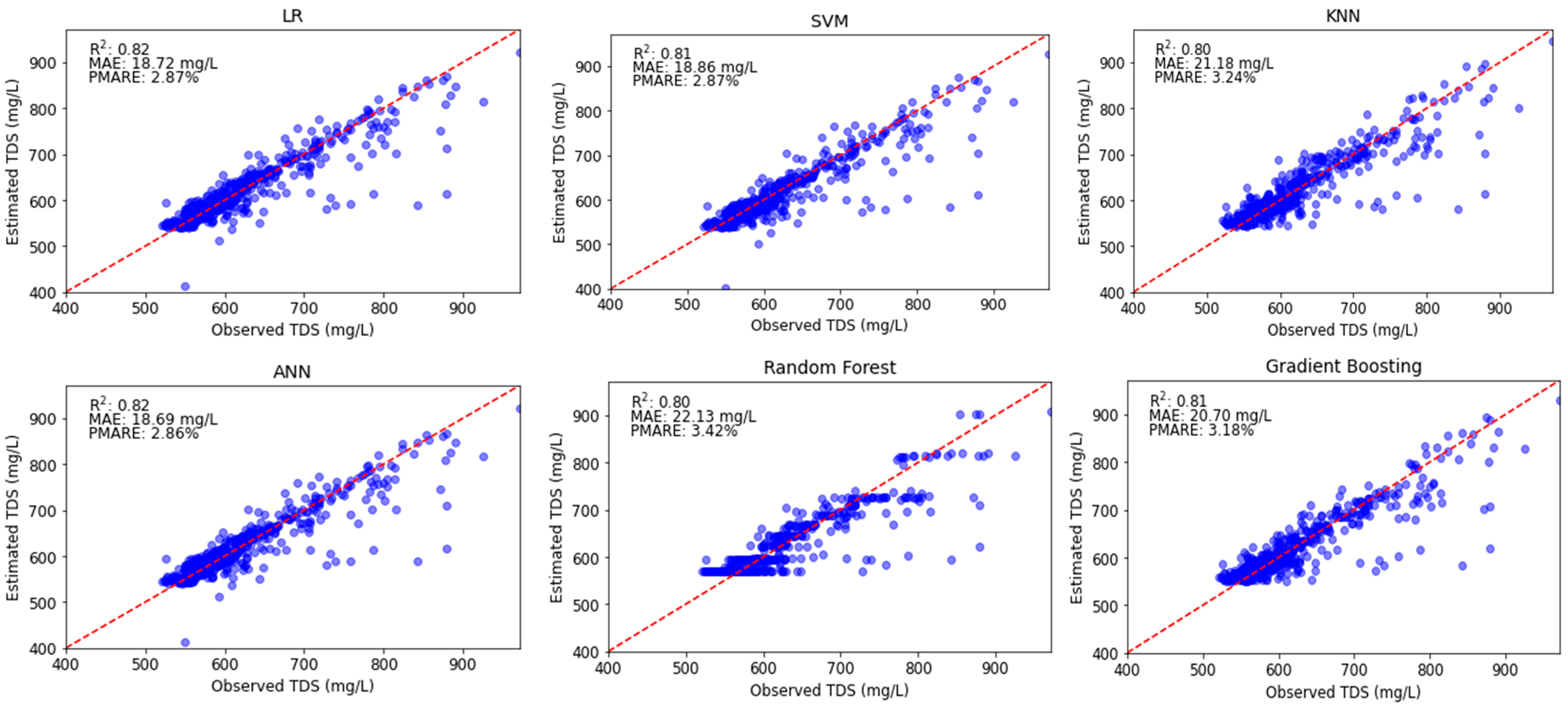
The results of the model evaluation for the unseen data (external validation), which represents potential estimates from real-life scenarios, are further presented using scatterplots, as shown in Figure 5, with a 45° bisector line to help researchers and decision-makers to visualize and interpret the model performance. The 45° bisector line aids in representing the perfect estimations. Best-performing models have the sample points lying around the bisector line, indicating best estimates [64]. From the plots, it is shown that all models perform similarly, with R2 ranging from 77 to 82%, with standalone models such as LR and ANN having the highest values of 82%, which is contrary to many studies reporting ensemble methods such as the RF and XGBoost to be best-performing models compared to standalone methods such as ANN, SVM, and LR [57,111,114], although studies such as [115,116] also found standalone ANN models to be better performers of WQPs than ensemble methods such as the RF. The findings from this study, therefore, mean that considering just one or few metrics in assessing the model performance may not necessarily give a better insight into the actual performance and that ensemble ML does not necessarily perform better than the standalone ML in every scenario. The superior performance of the standalone models such as the LR and the ANN on the external validation dataset in this study could be due to the simplicity of the relationships between the variables, particularly between TDS and EC [27].
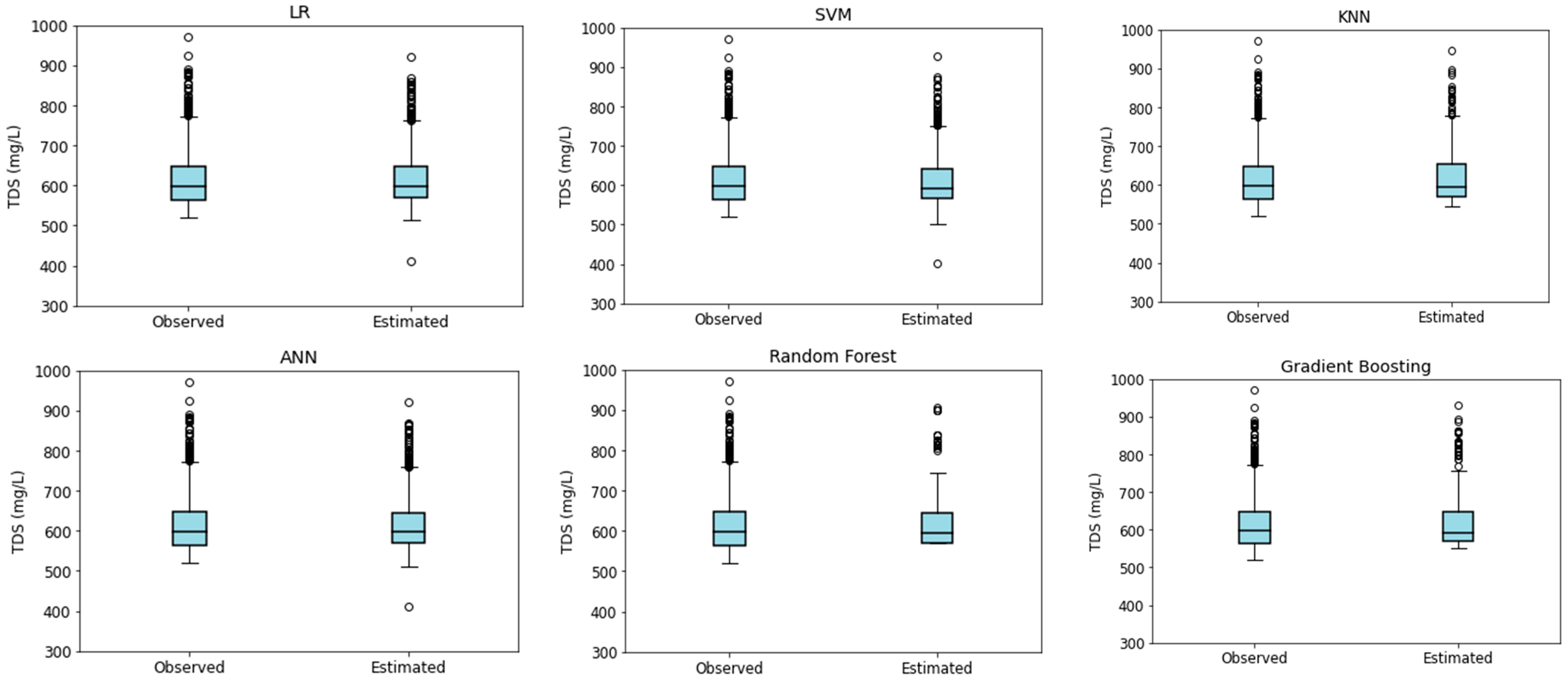
Boxplots used to visualize and compare the spread in the observed and estimated TDS concentrations for the ML models using the external validation are presented in Figure 6. The plots show the median (50th percentile) and other percentiles of TDS concentrations. The median value is displayed by the horizontal line inside the box, and the box indicates the interquartile range, or the values between the 25th and 75th percentiles, while the whiskers are the extension line from the first and third quartiles before the outliers [64]. The boxplots aid in further investigations and examinations of the model performance; with the boxplots, we gain further understanding of the performance of each model for estimating TDS. Models with more consistent and precise predictions are indicated with lower interquartile ranges and narrower whiskers. On the other hand, models with bigger whiskers and wider interquartile ranges imply increased variability and possible inaccuracies in the estimated TDS levels. The models accurately capture the extreme values, i.e., low and high TDS values, with the capture being prominent in the superior-performing models [64]. The findings from the boxplots can serve as a guide to further research or modeling technique improvements as well as aid in the selection of the best models for TDS estimation assignments.
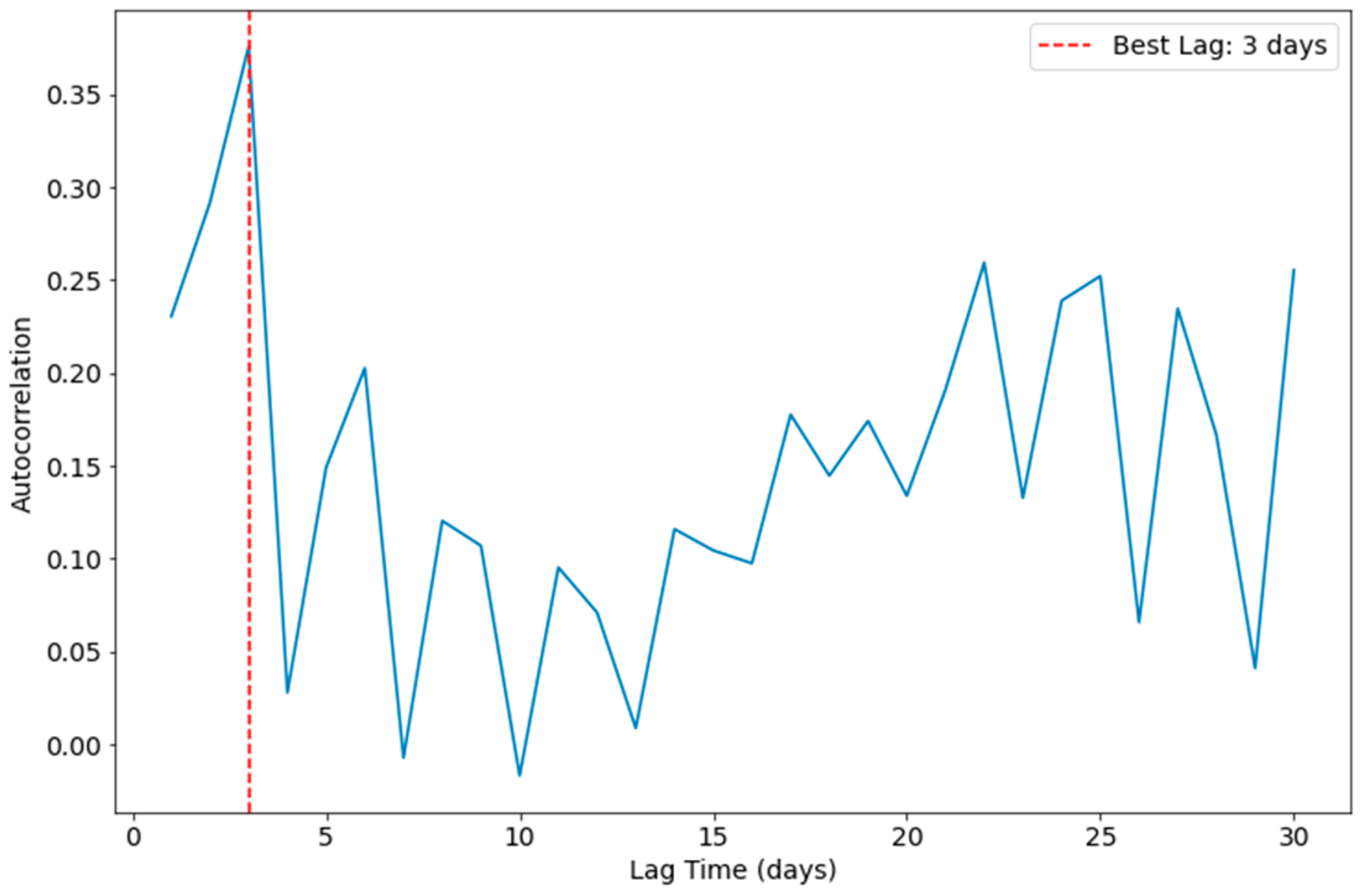
The time series of the observed and estimated TDS were produced to visually inspect the performance of the model. We used a lag time of 3 days to hypothetically account for the time it takes for the changes in EC and temperature to have an impact on the TDS concentration. This is important to minimize the significant irregularities between the predicted and observed TDS values and to accurately depict the temporally changing dynamics of the lake’s water system. To determine the optimal lag time to use, we based our analysis on how frequently the TDS concentration changes in the lake using autocorrelation of TDS values at different lag times, as presented by Equation (9). The lag time at which the highest autocorrelation occurs was taken as the period in which the change in the TDS is most apparent or pronounced [17,117,118,119], as presented in Figure 7.
p k = C o v ( X t , X t z ) σ t σ t z ,
where Cov (Xt, Xt−z,) are the covariances between the time series at time t and the lagged time (t − z), and σt and σt−z are the standard deviations for the time series at time t and lagged time, t − z. Values range from −1 to 1, with 1 meaning perfect positive correlations [17,118].
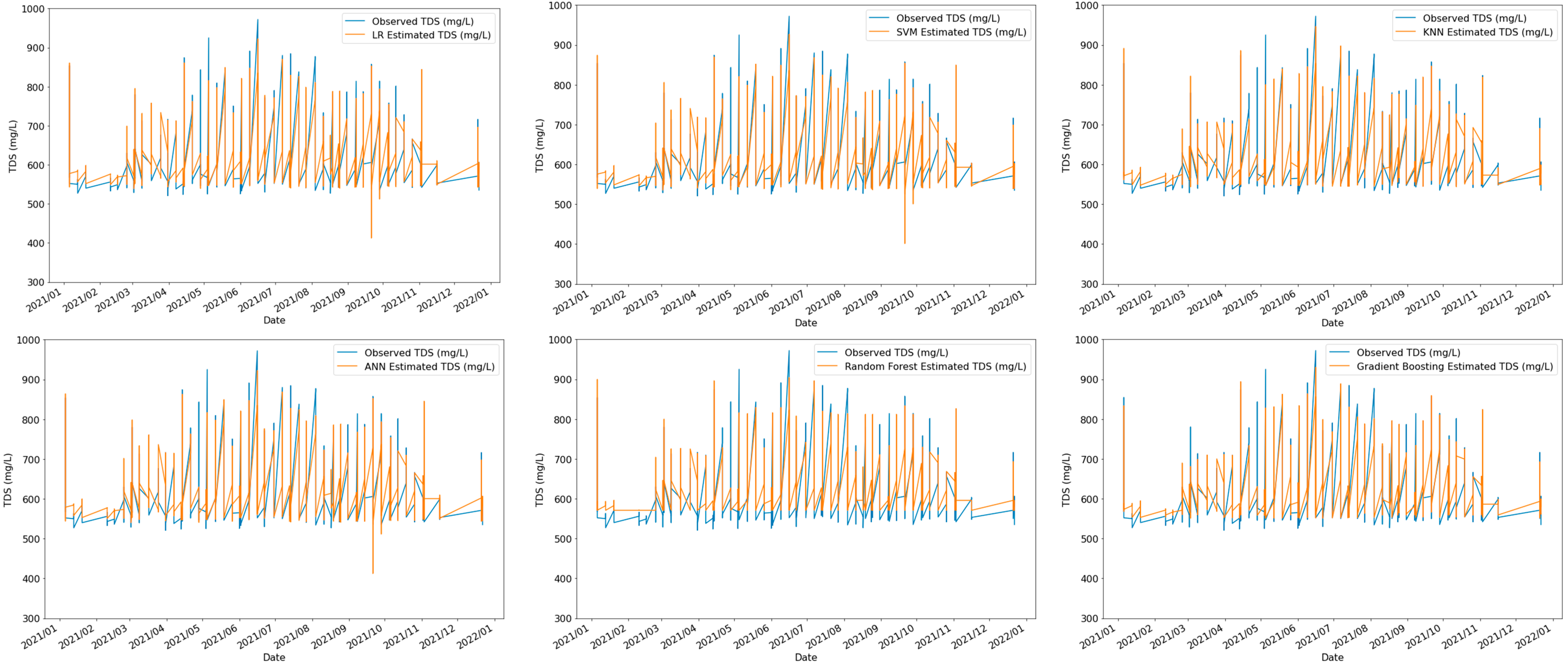
The time series of the observed and estimated TDS with the 3-day optimal lag time is presented in Figure 8.
The plots illustrate the performance of the models in estimating TDS concentration over the period under study. The observed and estimated TDS concentrations (using the external validation datasets) are presented in blue and orange colors, respectively, for visual temporal comparisons. If the estimated values closely match the observed values, the model is likely performing effectively and correctly identifying the fundamental patterns and trends in the data. Similarly, if the estimated values are routinely distant from the observed values, this indicates that the model is not performing effectively and may need to be improved. The time series plots, therefore, provide an opportunity in understanding the performance of each model in capturing the temporal trends and patterns in the TDS concentration. It is observed from the plots that modeled and observed values show similar trends, patterns, rises, and drops in the TDS, an indication of the potential of the models in the accurate detection of the temporal changes of the TDS. Comparing the time series plots for each model offers a great perspective on their performance. It is evident from the plots that the LR and GBM, respectively, for the standalone and ensemble models perform much more accurately compared to the other models.
Researchers and decision-makers can rely on these plots to understand and compare the potential of different models in detecting temporal changes of TDS.
Overall, these plots can help guide further improvement and optimization of the ML models by offering insightful information on how effectively the algorithms can estimate TDS concentration over time.

4. Conclusions

This study was aimed at estimating TDS concentration using EC and temperature. EC and TDS are indicators of the salinity level of a water body. The temperature has also been found to have an influence on the solubility of ions and hence the salinity of the water. Measurement of EC and temperature are simpler and straightforward compared with TDS measurement. TDS measurement is, however, paramount as it provides a more thorough explanation of the water quality than the EC and temperature. Conducting TDS analysis in the water requires detailed and elaborative field sampling and laboratory gravimetric experiments which are cost-prohibitive. Studies have discovered correlations between TDS and EC; these interactions are, however, not always linear and are dependent on the material content and salinity of the water.
This study, therefore, utilized several standalone models, such as LR, SVM, KNN, and ANN, and ensemble models, such as bagging, GBM, ET, RF, and XGBoost, for estimating TDS from conductivity and temperature. Different performance metrics were used to evaluate the performance of the models, including the R2, RMSE, MAE, PMARE, SI, NSE, and PBIAS.
The results obtained show, for the external validation dataset, standalone models producing R2 and RMSE of 0.80–0.82 and 33.10–35.12 mg/L, respectively, while the ensemble models produced R2 and RMSE of 0.77–0.81 and 34.19–37.69 mg/L, respectively. We summarized the performance of the models using the ranks and found that the LR has the superior prediction of all the models on the external validation dataset although it showed a weaker prediction on the training dataset, possibly due to overfitting, while the GBM showed superior prediction in the training and testing phase of the model. The LR provided a reliable and robust estimation of the external validation dataset, possibly due to the existence of the simplicity in the relations between the variables, particularly between TDS and EC [27].
Comparing the overall performance of all models across the three different dataset stages saw ensemble methods such as the GB and XGBoost outperforming all the models, with overall performance average rank of 3.1 and 3.4 indicating the overall superiority for TDS due to its robustness to overfitting and underlying algorithms described in Section 2.3.2. Results obtained indicate the potential of utilizing this ML in estimating TDS concentration across all the various stages of modeling (i.e., training, testing, and external validation).
Overall, the study showed the potential of utilizing a cost-effective ML in models to estimate TDS in water using EC and temperature. The developed models can be applied in cost-effective water quality management efforts. These models could also aid in environmental monitoring assisted programs, providing early warning alerts (when estimated TDS exceeds the regulatory limits), resource allocations, and water hazard assessments, ultimately adding to efforts in ensuring water sustainability.
The performance of each model varied among the models since each model presented strengths and limitations. An example is the case of the LR, which assumes the existence of linear association among the variables. The absence of such a relationship may limit the ability to fit it as a model for accurate predictions. All the models also rely on hyperparameters, and selecting the optimal hyperparameters for the models may also contribute to their performance. This study used grid search with five folds to carry out cross-validation for optimizing the hyperparameters, which may contribute to the model performance. Some studies have that found cross-validations with 10 folds provides accurate estimations, although they are computing-intensive and time-consuming, particularly for a large dataset.
Further analysis may be required to validate the models to make them robust using datasets collected from different water bodies for the generalization of the model. Additionally, there is a need to explore other techniques that may improve the performance reliability, accuracy, and usefulness, including increasing the number of folds used in the cross-validation.

Author Contributions

G.E.A. contributed to the conceptualization, methodology, analysis, and original and final writing of the manuscript. H.S. and S.A. both contributed to the conceptualization and writing—review and editing, and supervision of the manuscript. All authors have read and agreed to the published version of the manuscript.

Funding

This research received no external funding.

Data Availability Statement

Data used for this study is available upon request.

Acknowledgments

The publication fees for this article were supported by the UNLV MSI Open Article Fund. The authors would like to acknowledge Captain Scott H. Schiefer of the City of Las Vegas and David James of the Civil and Environmental Engineering and Construction Department at the University of Nevada, Las Vegas (UNLV), for their help in obtaining the water quality data for this study. Many thanks to Charles Adjovu for his help in explaining some ML principles and models.

Conflicts of Interest

The authors declare no conflict of interest.

References

  1. Venkatesan, A.K.; Ahmad, S.; Johnson, W.; Batista, J.R. Salinity Reduction and Energy Conservation in Direct and Indirect Potable Water Reuse. Desalination 2011, 272, 120–127. [Google Scholar] [CrossRef]
  2. Adjovu, G.E.; Stephen, H.; Ahmad, S. Monitoring of Total Dissolved Solids Using Remote Sensing Band Reflectance and Salinity Indices: A Case Study of the Imperial County Section, AZ-CA, of the Colorado River. In Proceedings of the World Environmental and Water Resources Congress 2022, Atlanta, Georgia, 5–8 June 2022. [Google Scholar] [CrossRef]
  3. Adjovu, G.E.; Stephen, H.; Ahmad, S. Spatial and Temporal Dynamics of Key Water Quality Parameters in a Thermal Stratified Lake Ecosystem: The Case Study of Lake Mead. Earth 2023, 4, 461–502. [Google Scholar] [CrossRef]
  4. Wheeler, K.G.; Udall, B.; Wang, J.; Kuhn, E.; Salehabadi, H.; Schmidt, J.C. What Will It Take to Stabilize the Colorado River? Science 2022, 377, 373–375. [Google Scholar] [CrossRef] [PubMed]
  5. Rahaman, M.M.; Thakur, B.; Kalra, A.; Ahmad, S. Modeling of GRACE-Derived Groundwater Information in the Colorado River Basin. Hydrology 2019, 6, 19. [Google Scholar] [CrossRef] [Green Version]
  6. Venkatesan, A.K.; Ahmad, S.; Batista, J.R.; Johnson, W.S. Total Dissolved Solids Contribution to the Colorado River Associated with the Growth of Las Vegas Valley. In Proceedings of the World Environmental and Water Resources Congress 2010, Providence, RI, USA, 16–20 May 2010; pp. 3376–3385. [Google Scholar] [CrossRef]
  7. Shaikh, T.A.; Adjovu, G.E.; Stephen, H.; Ahmad, S. Impacts of Urbanization on Watershed Hydrology and Runoff Water Quality of a Watershed: A Review. In Proceedings of the World Environmental and Water Resources Congress 2023, Henderson, NV, USA, 21–25 May 2023; Volume 1, pp. 1271–1283. Available online: https://ascelibrary.org/doi/10.1061/9780784484852.116 (accessed on 25 May 2023).
  8. Sowby, R.B.; Hotchkiss, R.H. Minimizing Unintended Consequences of Water Resources Decisions. J. Water Resour. Plan. Manag. 2022, 148, 02522007. [Google Scholar] [CrossRef]
  9. Shope, C.L.; Gerner, S.J. Assessment of Dissolved-Solids Loading to the Colorado River in the Paradox Basin between the Dolores River and Gypsum Canyon, Utah; U.S. Geological Survey Scientific Investigations Report 2014-5031; U.S. Geological Survey: Reston, VA, USA, 2016. [CrossRef] [Green Version]
  10. Nauman, T.W.; Ely, C.P.; Miller, M.P.; Duniway, M.C. Salinity Yield Modeling of the Upper Colorado River Basin Using 30-m Resolution Soil Maps and Random Forests. Water Resour. Res. 2019, 55, 4954–4973. [Google Scholar] [CrossRef]
  11. Tillman, F.D.; Day, N.K.; Miller, M.P.; Miller, O.L.; Rumsey, C.A.; Wise, D.R.; Longley, P.C.; McDonnell, M.C. A Review of Current Capabilities and Science Gaps in Water Supply Data, Modeling, and Trends for Water Availability Assessments in the Upper Colorado River Basin. Water 2022, 14, 3813. [Google Scholar] [CrossRef]
  12. Adjovu, G.E.; Stephen, H.; Ahmad, S. Spatiotemporal Variability in Total Dissolved Solids and Total Suspended Solids along the Colorado River. Hydrology 2023, 10, 125. [Google Scholar] [CrossRef]
  13. Khan, I.; Khan, A.; Khan, M.S.; Zafar, S.; Hameed, A.; Badshah, S.; Rehman, S.U.; Ullah, H.; Yasmeen, G. Impact of City Effluents on Water Quality of Indus River: Assessment of Temporal and Spatial Variations in the Southern Region of Khyber Pakhtunkhwa, Pakistan. Environ. Monit. Assess. 2018, 190, 267. [Google Scholar] [CrossRef]
  14. Adjovu, G.E.; Stephen, H.; James, D.; Ahmad, S. Overview of the Application of Remote Sensing in Effective Monitoring of Water Quality Parameters. Remote Sens. 2023, 15, 1938. [Google Scholar] [CrossRef]
  15. U.S. EPA. 2018 Edition of the Drinking Water Standards and Health Advisories Tables; U.S. EPA: Washington, DC, USA, 2018. Available online: https://www.epa.gov/system/files/documents/2022-01/dwtable2018.pdf (accessed on 25 May 2023).
  16. EPA. National Primary Drinking Water Guidelines; U.S. EPA: Washington, DC, USA, 2009. Available online: https://www.epa.gov/sites/production/files/2016-06/documents/npwdr_complete_table.pdf (accessed on 25 May 2023).
  17. Mejía Ávila, D.; Torres-Bejarano, F.; Martínez Lara, Z. Spectral Indices for Estimating Total Dissolved Solids in Freshwater Wetlands Using Semi-Empirical Models. A Case Study of Guartinaja and Momil Wetlands. Int. J. Remote Sens. 2022, 43, 2156–2184. [Google Scholar] [CrossRef]
  18. Hach Solids (Total & Dissolved). Available online: https://www.hach.com/parameters/solids (accessed on 25 May 2023).
  19. Butler, B.A.; Ford, R.G. Evaluating Relationships between Total Dissolved Solids (TDS) and Total Suspended Solids (TSS) in a Mining-Influenced Watershed. Mine Water Environ. 2018, 31, 18–30. [Google Scholar] [CrossRef]
  20. Shareef, M.A.; Toumi, A.; Khenchaf, A. Estimating of Water Quality Parameters Using SAR and Thermal Microwave Remote Sensing Data. In Proceedings of the 2nd International Conference on Advanced Technologies for Signal and Image Processing (ATSIP), Monastir, Tunisia, 21–23 March 2016; pp. 586–590. [Google Scholar] [CrossRef]
  21. Ladwig, R.; Rock, L.A.; Dugan, H.A. Impact of Salinization on Lake Stratification and Spring Mixing. Limnol. Oceanogr. Lett. 2021, 8, 93–102. [Google Scholar] [CrossRef]
  22. Fant, C.; Srinivasan, R.; Boehlert, B.; Rennels, L.; Chapra, S.C.; Strzepek, K.M.; Corona, J.; Allen, A.; Martinich, J. Climate Change Impacts on Us Water Quality Using Two Models: HAWQS and US Basins. Water 2017, 9, 118. [Google Scholar] [CrossRef] [Green Version]
  23. Denys, L. Incomplete Spring Turnover in Small Deep Lakes in SE Michigan. McNair Sch. Res. J. 2010, 2, 10. [Google Scholar]
  24. Sauck, W.A. A Model for the Resistivity Structure of LNAPL Plumes and Their Environs in Sandy Sediments. J. Appl. Geophys. 2000, 44, 151–165. [Google Scholar] [CrossRef]
  25. Jiang, L.; Liu, Y.; Hu, X.; Zeng, G.; Wang, H.; Zhou, L.; Tan, X.; Huang, B.; Liu, S.; Liu, S. The Use of Microbial-Earthworm Ecofilters for Wastewater Treatment with Special Attention to Influencing Factors in Performance: A Review. Bioresour. Technol. 2016, 200, 999–1007. [Google Scholar] [CrossRef]
  26. Chapter 5—Sampling. In NPDES Compliance Inspection Manual; U.S. Environmental Protection Agency: Washington, DC, USA, 2017. Available online: https://www.epa.gov/sites/default/files/2017-03/documents/npdesinspect-chapter-05.pdf (accessed on 25 May 2023).
  27. Rusydi, A.F. Correlation between Conductivity and Total Dissolved Solid in Various Type of Water: A Review. IOP Conf. Ser. Earth Environ. Sci. 2018, 118, 012019. [Google Scholar] [CrossRef]
  28. Rodger, B.; Baird, A.D.; Eaton, E.W.R. Standard Methods for the Examination of Water and Wastewater; American Public Health Association, American Water Works Association, Water Environment Federation: Washington, DC, USA, 2017; pp. 1–1545. [Google Scholar]
  29. Shareef, M.A.; Toumi, A.; Khenchaf, A. Estimation and Characterization of Physical and Inorganic Chemical Indicators of Water Quality by Using SAR Images. SAR Image Anal. Model. Technol. XV 2015, 9642, 96420U. [Google Scholar] [CrossRef]
  30. Woodside, J. What Is the Difference among Turbidity, TDS, and TSS? Available online: https://www.ysi.com/ysi-blog/water-blogged-blog/2022/05/understanding-turbidity-tds-and-tss (accessed on 25 May 2023).
  31. Gholizadeh, M.H.; Melesse, A.M.; Reddi, L. A Comprehensive Review on Water Quality Parameters Estimation Using Remote Sensing Techniques. Sensors 2016, 16, 1298. [Google Scholar] [CrossRef] [PubMed] [Green Version]
  32. Adjovu, G.E.; Ali Shaikh, T.; Stephen, H.; Ahmad, S. Utilization of Machine Learning Models and Satellite Data for the Estimation of Total Dissolved Solids in the Colorado River System. In Proceedings of the World Environmental and Water Resources Congress 2023, Henderson, NV, USA, 21–24 May 2023; Volume 1, pp. 1147–1160. [Google Scholar]
  33. Taylor, M.; Elliott, H.A.; Navitsky, L.O. Relationship between Total Dissolved Solids and Electrical Conductivity in Marcellus Hydraulic Fracturing Fluids. Water Sci. Technol. 2018, 77, 1998–2004. [Google Scholar] [CrossRef]
  34. Kupssinskü, L.S.; Guimarães, T.T.; De Souza, E.M.; Zanotta, D.C.; Veronez, M.R.; Gonzaga, L.; Mauad, F.F. A Method for Chlorophyll-a and Suspended Solids Prediction through Remote Sensing and Machine Learning. Sensors 2020, 20, 2125. [Google Scholar] [CrossRef] [Green Version]
  35. Peterson, K.T.; Sagan, V.; Sidike, P.; Cox, A.L.; Martinez, M. Suspended Sediment Concentration Estimation from Landsat Imagery along the Lower Missouri and Middle Mississippi Rivers Using an Extreme Learning Machine. Remote Sens. 2018, 10, 1503. [Google Scholar] [CrossRef] [Green Version]
  36. Yang, H.; Kong, J.; Hu, H.; Du, Y.; Gao, M.; Chen, F. A Review of Remote Sensing for Water Quality Retrieval: Progress and Challenges. Remote Sens. 2022, 14, 1770. [Google Scholar] [CrossRef]
  37. Wakjira, T.G.; Rahmzadeh, A.; Alam, M.S.; Tremblay, R. Explainable Machine Learning Based Efficient Prediction Tool for Lateral Cyclic Response of Post-Tensioned Base Rocking Steel Bridge Piers. Structures 2022, 44, 947–964. [Google Scholar] [CrossRef]
  38. Najafzadeh, M.; Ghaemi, A.; Emamgholizadeh, S. Prediction of Water Quality Parameters Using Evolutionary Computing-Based Formulations. Int. J. Environ. Sci. Technol. 2019, 16, 6377–6396. [Google Scholar] [CrossRef]
  39. Najafzadeh, M.; Ghaemi, A. Prediction of the Five-Day Biochemical Oxygen Demand and Chemical Oxygen Demand in Natural Streams Using Machine Learning Methods. Environ. Monit. Assess. 2019, 191, 380. [Google Scholar] [CrossRef]
  40. Kaur, H.; Malhi, A.K.; Pannu, H.S. Machine Learning Ensemble for Neurological Disorders. Neural Comput. Appl. 2020, 32, 12697–12714. [Google Scholar] [CrossRef]
  41. Singh, A.K. Impact of the Coronavirus Pandemic on Las Vegas Strip Gaming Revenue. J. Gambl. Bus. Econ. 2021, 14. [Google Scholar] [CrossRef]
  42. Kutty, A.A.; Wakjira, T.G.; Kucukvar, M.; Abdella, G.M.; Onat, N.C. Urban Resilience and Livability Performance of European Smart Cities: A Novel Machine Learning Approach. J. Clean. Prod. 2022, 378, 134203. [Google Scholar] [CrossRef]
  43. Hope, T.M.H. Linear Regression. In Machine Learning; Elsevier: Amsterdam, The Netherlands, 2020; pp. 67–81. ISBN 9780128157398. [Google Scholar]
  44. Li, S.; Song, K.; Wang, S.; Liu, G.; Wen, Z.; Shang, Y.; Lyu, L.; Chen, F.; Xu, S.; Tao, H.; et al. Quantification of Chlorophyll-a in Typical Lakes across China Using Sentinel-2 MSI Imagery with Machine Learning Algorithm. Sci. Total Environ. 2021, 778, 146271. [Google Scholar] [CrossRef]
  45. Najafzadeh, M.; Basirian, S. Evaluation of River Water Quality Index Using Remote Sensing and Artificial Intelligence Models. Remote Sens. 2023, 15, 2359. [Google Scholar] [CrossRef]
  46. Najafzadeh, M.; Homaei, F.; Farhadi, H. Reliability Assessment of Water Quality Index Based on Guidelines of National Sanitation Foundation in Natural Streams: Integration of Remote Sensing and Data-Driven Models; Springer: Dordrecht, The Netherlands, 2021; Volume 54, ISBN 0123456789. [Google Scholar]
  47. Melesse, A.M.; Ahmad, S.; McClain, M.E.; Wang, X.; Lim, Y.H. Suspended Sediment Load Prediction of River Systems: An Artificial Neural Network Approach. Agric. Water Manag. 2011, 98, 855–866. [Google Scholar] [CrossRef]
  48. Bayati, M.; Danesh-Yazdi, M. Mapping the Spatiotemporal Variability of Salinity in the Hypersaline Lake Urmia Using Sentinel-2 and Landsat-8 Imagery. J. Hydrol. 2021, 595, 126032. [Google Scholar] [CrossRef]
  49. Bedi, S.; Samal, A.; Ray, C.; Snow, D. Comparative Evaluation of Machine Learning Models for Groundwater Quality Assessment. Environ. Monit. Assess. 2020, 192, 776. [Google Scholar] [CrossRef] [PubMed]
  50. Adjovu, G.E.; Ahmad, S.; Stephen, H. Analysis of Suspended Material in Lake Mead Using Remote Sensing Indices. In Proceedings of the World Environmental and Water Resources Congress 2021, Virtual, 7–11 June 2021. [Google Scholar]
  51. Edalat, M.M.; Stephen, H. Socio-Economic Drought Assessment in Lake Mead, USA, Based on a Multivariate Standardized Water-Scarcity Index. Hydrol. Sci. J. 2019, 64, 555–569. [Google Scholar] [CrossRef]
  52. Rosen, M.R.; Turner, K.; Goodbred, S.L.; Miller, J.M. A Synthesis of Aquatic Science for Management of Lakes Mead and Mohave; US Geological Survey: Reston, VA, USA, 2012; ISBN 9781411335271.
  53. Morfín, O. Effects of System Conservation on Salinity in Lake Mead. Available online: https://www.multi-statesalinitycoalition.com/wp-content/uploads/2017-Morfin.pdf (accessed on 25 May 2023).
  54. Venkatesan, A.K.; Ahmad, S.; Johnson, W.; Batista, J.R. Systems Dynamic Model to Forecast Salinity Load to the Colorado River Due to Urbanization within the Las Vegas Valley. Sci. Total Environ. 2011, 409, 2616–2625. [Google Scholar] [CrossRef] [PubMed]
  55. Dunbar, M.; Harney, S.; Morgan, D.; LaRance, D.; Speaks, F. Lake Mead and Las Vegas Wash 2019 Annual Report; City of Las Vegas, Clark County Water Reclamation District, City of Henderson City, City of North Las Vegas. 2020. Available online: https://drive.google.com/file/d/1XSWvEf74XX2KULmsYQ3ZHRAsOo8RsXN8/view?usp=sharing (accessed on 25 May 2023).
  56. Di Napoli, M.; Carotenuto, F.; Cevasco, A.; Confuorto, P.; Di Martire, D.; Firpo, M.; Pepe, G.; Raso, E.; Calcaterra, D. Machine Learning Ensemble Modelling as a Tool to Improve Landslide Susceptibility Mapping Reliability. Landslides 2020, 17, 1897–1914. [Google Scholar] [CrossRef]
  57. Zounemat-Kermani, M.; Batelaan, O.; Fadaee, M.; Hinkelmann, R. Ensemble Machine Learning Paradigms in Hydrology: A Review. J. Hydrol. 2021, 598, 126266. [Google Scholar] [CrossRef]
  58. Wakjira, T.G.; Ibrahim, M.; Ebead, U.; Alam, M.S. Explainable Machine Learning Model and Reliability Analysis for Flexural Capacity Prediction of RC Beams Strengthened in Flexure with FRCM. Eng. Struct. 2022, 255, 113903. [Google Scholar] [CrossRef]
  59. Chen, J.; de Hoogh, K.; Gulliver, J.; Hoffmann, B.; Hertel, O.; Ketzel, M.; Bauwelinck, M.; van Donkelaar, A.; Hvidtfeldt, U.A.; Katsouyanni, K.; et al. A Comparison of Linear Regression, Regularization, and Machine Learning Algorithms to Develop Europe-Wide Spatial Models of Fine Particles and Nitrogen Dioxide. Environ. Int. 2019, 130, 104934. [Google Scholar] [CrossRef]
  60. Maulud, D.; Abdulazeez, A.M. A Review on Linear Regression Comprehensive in Machine Learning. J. Appl. Sci. Technol. Trends 2020, 1, 140–147. [Google Scholar] [CrossRef]
  61. Ansari, M.; Akhoondzadeh, M. Mapping Water Salinity Using Landsat-8 OLI Satellite Images (Case Study: Karun Basin Located in Iran). Adv. Sp. Res. 2020, 65, 1490–1502. [Google Scholar] [CrossRef]
  62. Rong, S.; Bao-Wen, Z. The Research of Regression Model in Machine Learning Field. MATEC Web Conf. 2018, 176, 8–11. [Google Scholar] [CrossRef] [Green Version]
  63. Kavitha, S.; Varuna, S.; Ramya, R. A Comparative Analysis on Linear Regression and Support Vector Regression. In Proceedings of the 2016 Online International Conference on Green Engineering and Technologies (IC-GET) 2016, Coimbatore, India, 19 November 2016. [Google Scholar] [CrossRef]
  64. Ahmad, S.; Kalra, A.; Stephen, H. Estimating Soil Moisture Using Remote Sensing Data: A Machine Learning Approach. Adv. Water Resour. 2010, 33, 69–80. [Google Scholar] [CrossRef]
  65. Rodriguez-Galiano, V.; Sanchez-Castillo, M.; Chica-Olmo, M.; Chica-Rivas, M. Machine Learning Predictive Models for Mineral Prospectivity: An Evaluation of Neural Networks, Random Forest, Regression Trees and Support Vector Machines. Ore Geol. Rev. 2015, 71, 804–818. [Google Scholar] [CrossRef]
  66. Banadkooki, F.B.; Ehteram, M.; Panahi, F.; Sammen, S.S.; Othman, F.B.; EL-Shafie, A. Estimation of Total Dissolved Solids (TDS) Using New Hybrid Machine Learning Models. J. Hydrol. 2020, 587, 124989. [Google Scholar] [CrossRef]
  67. Rumora, L.; Miler, M.; Medak, D. Impact of Various Atmospheric Corrections on Sentinel-2 Land Cover Classification Accuracy Using Machine Learning Classifiers. ISPRS Int. J. Geo-Inf. 2020, 9, 277. [Google Scholar] [CrossRef] [Green Version]
  68. Phyo, P.P.; Byun, Y.C.; Park, N. Short-Term Energy Forecasting Using Machine-Learning-Based Ensemble Voting Regression. Symmetry 2022, 14, 160. [Google Scholar] [CrossRef]
  69. Alexei Botchkarev Performance Metrics (Error Measures) in Machine Learning Regression, Forecasting and Prognostics: Properties and Typology. J. Chem. Inf. Model. 1981, 53, 1689–1699.
  70. Kumar, V.; Sharma, A.; Bhardwaj, R.; Thukral, A.K. Water Quality of River Beas, India, and Its Correlation with Reflectance Data. J. Water Chem. Technol. 2020, 42, 134–141. [Google Scholar] [CrossRef]
  71. Kumar, V.; Sharma, A.; Chawla, A.; Bhardwaj, R.; Thukral, A.K. Water Quality Assessment of River Beas, India, Using Multivariate and Remote Sensing Techniques. Environ. Monit. Assess. 2016, 188, 137. [Google Scholar] [CrossRef]
  72. Mosavi, A.; Ozturk, P.; Chau, K.W. Flood Prediction Using Machine Learning Models: Literature Review. Water 2018, 10, 1536. [Google Scholar] [CrossRef] [Green Version]
  73. Song, K.; Li, L.; Wang, Z.; Liu, D.; Zhang, B.; Xu, J.; Du, J.; Li, L.; Li, S.; Wang, Y. Retrieval of Total Suspended Matter (TSM) and Chlorophyll-a (Chl-a) Concentration from Remote-Sensing Data for Drinking Water Resources. Environ. Monit. Assess. 2011, 184, 1449–1470. [Google Scholar] [CrossRef] [PubMed]
  74. Zhang, C.; Ma, Y. Ensemble Machine Learning: Methods and Applications; Zhang, C., Ma, Y., Eds.; Springer: Boston, MA, USA, 2012; ISBN 978-1-4419-9325-0. [Google Scholar]
  75. Rocca, J. Ensemble Methods: Bagging, Boosting and Stacking. Available online: https://towardsdatascience.com/ensemble-methods-bagging-boosting-and-stacking-c9214a10a205 (accessed on 25 May 2023).
  76. Scikit Learn Hyperparameter Tuning. Available online: https://inria.github.io/scikit-learn-mooc/python_scripts/ensemble_hyperparameters.html (accessed on 25 May 2023).
  77. Geurts, P.; Ernst, D.; Wehenkel, L. Extremely Randomized Trees. Mach. Learn. 2006, 63, 3–42. [Google Scholar] [CrossRef] [Green Version]
  78. Livingston, F. Implementation of Breiman’s Random Forest Machine Learning Algorithm. Mach. Learn. J. Pap. 2005, Fall, 1–13. [Google Scholar]
  79. Tillman, F.D.; Anning, D.W.; Heilman, J.A.; Buto, S.G.; Miller, M.P. Managing Salinity in Upper Colorado River Basin Streams: Selecting Catchments for Sediment Control Efforts Using Watershed Characteristics and Random Forests Models. Water 2018, 10, 676. [Google Scholar] [CrossRef] [Green Version]
  80. Wolff, S.; O’Donncha, F.; Chen, B. Statistical and Machine Learning Ensemble Modelling to Forecast Sea Surface Temperature. J. Mar. Syst. 2020, 208, 103347. [Google Scholar] [CrossRef]
  81. Imen, S.; Chang, N.B.; Yang, Y.J. Developing the Remote Sensing-Based Early Warning System for Monitoring TSS Concentrations in Lake Mead. J. Environ. Manag. 2015, 160, 73–89. [Google Scholar] [CrossRef]
  82. Wakjira, T.G.; Abushanab, A.; Ebead, U.; Alnahhal, W. FAI: Fast, Accurate, and Intelligent Approach and Prediction Tool for Flexural Capacity of FRP-RC Beams Based on Super-Learner Machine Learning Model. Mater. Today Commun. 2022, 33, 104461. [Google Scholar] [CrossRef]
  83. Sciikit Learn Sklearn.Model_selection.KFold. Available online: https://scikit-learn.org/stable/modules/generated/sklearn.model_selection.KFold.html (accessed on 25 May 2023).
  84. Wang, Z.; Lei, Y.; Cui, H.; Miao, H.; Zhang, D.; Wu, Z.; Liu, G. Enhanced RBF Neural Network Metamodelling Approach Assisted by Sliced Splitting-Based K-Fold Cross-Validation and Its Application for the Stiffened Cylindrical Shells. Aerosp. Sci. Technol. 2022, 124, 107534. [Google Scholar] [CrossRef]
  85. Shah, M.I.; Javed, M.F.; Abunama, T. Proposed Formulation of Surface Water Quality and Modelling Using Gene Expression, Machine Learning, and Regression Techniques. Environ. Sci. Pollut. Res. 2021, 28, 13202–13220. [Google Scholar] [CrossRef] [PubMed]
  86. Saberioon, M.; Brom, J.; Nedbal, V.; Souček, P.; Císař, P. Chlorophyll-a and Total Suspended Solids Retrieval and Mapping Using Sentinel-2A and Machine Learning for Inland Waters. Ecol. Indic. 2020, 113, 106236. [Google Scholar] [CrossRef]
  87. Dritsas, E.; Trigka, M. Efficient Data-Driven Machine Learning Models for Water Quality Prediction. Computation 2023, 11, 16. [Google Scholar] [CrossRef]
  88. Leigh, C.; Kandanaarachchi, S.; McGree, J.M.; Hyndman, R.J.; Alsibai, O.; Mengersen, K.; Peterson, E.E. Predicting Sediment and Nutrient Concentrations from High-Frequency Water-Quality Data. PLoS ONE 2019, 14, e0215957. [Google Scholar] [CrossRef] [PubMed] [Green Version]
  89. Mahanty, B.; Lhamo, P.; Sahoo, N.K. Inconsistency of PCA-Based Water Quality Index–Does It Reflect the Quality? Sci. Total Environ. 2023, 866, 161353. [Google Scholar] [CrossRef] [PubMed]
  90. Jung, K.; Bae, D.H.; Um, M.J.; Kim, S.; Jeon, S.; Park, D. Evaluation of Nitrate Load Estimations Using Neural Networks and Canonical Correlation Analysis with K-Fold Cross-Validation. Sustainability 2020, 12, 400. [Google Scholar] [CrossRef] [Green Version]
  91. Mamat, N.; Hamzah, M.F.; Jaafar, O. Hybrid Support Vector Regression Model and K-Fold Cross Validation for Water Quality Index Prediction in Langat River, Malaysia. bioRxiv 2021. [Google Scholar] [CrossRef]
  92. Normawati, D.; Ismi, D.P. K-Fold Cross Validation for Selection of Cardiovascular Disease Diagnosis Features by Applying Rule-Based Datamining. Signal Image Process. Lett. 2019, 1, 23–35. [Google Scholar] [CrossRef]
  93. Scikit Learn Supervised Learning-Scikit Learn Documentation. Available online: https://scikit-learn.org/0.23/supervised_learning.html (accessed on 25 May 2023).
  94. VanderPlas, J. Python Data Science Handbook; O’Reilly Media: Sebastopol, CA, USA, 2019; Volume 53, ISBN 9788578110796. [Google Scholar]
  95. Grus, J. Data Science from Scratch; O’Reilly Media: Sebastopol, CA, USA, 2019; Volume 1542, ISBN 9781492041139. [Google Scholar]
  96. Adjovu, G.E.; Gamble, R. Development of HEC-HMS Model for the Cane Creek Watershed. In Proceedings of the 22nd Tennessee Water Resources Symposium, Burns, TN, USA, 10–12 April 2019; Tennessee Section of the American Water Resources Association: Nashville, TN, USA; pp. 1C-2–1C-6. Available online: https://img1.wsimg.com/blobby/go/12ed7af3-57dc-468c-af58-da8360f35f16/downloads/Proceedings2019.pdf?ver=1618503482462 (accessed on 25 May 2023).
  97. Moriasi, D.N.; Arnold, J.G.; Van Liew, M.W.; Bingner, R.L.; Harmel, R.D.; Veith, T.L. Model Evaluation Guidelines for Systematic Quantification of Accuracy in Watershed Simulations. Trans. ASABE 2007, 50, 885–900. [Google Scholar] [CrossRef]
  98. da Silva, M.G.; de Aguiar Netto, A.d.O.; de Jesus Neves, R.J.; do Vasco, A.N.; Almeida, C.; Faccioli, G.G. Sensitivity Analysis and Calibration of Hydrological Modeling of the Watershed Northeast Brazil. J. Environ. Prot. 2015, 6, 837–850. [Google Scholar] [CrossRef] [Green Version]
  99. Chicco, D.; Warrens, M.J.; Jurman, G. The Coefficient of Determination R-Squared Is More Informative than SMAPE, MAE, MAPE, MSE and RMSE in Regression Analysis Evaluation. PeerJ Comput. Sci. 2021, 7, e623. [Google Scholar] [CrossRef] [PubMed]
  100. Saberi-Movahed, F.; Najafzadeh, M.; Mehrpooya, A. Receiving More Accurate Predictions for Longitudinal Dispersion Coefficients in Water Pipelines: Training Group Method of Data Handling Using Extreme Learning Machine Conceptions. Water Resour. Manag. 2020, 34, 529–561. [Google Scholar] [CrossRef]
  101. Adjovu, G.E. Evaluating the Performance of A GIS-Based Tool for Delineating Swales Along Two Highways in Tennessee. Ph.D. Thesis, Tennessee Technological University, Cookeville, TN, USA, 2020. [Google Scholar]
  102. Sun, K.; Rajabtabar, M.; Samadi, S.Z.; Rezaie-Balf, M.; Ghaemi, A.; Band, S.S.; Mosavi, A. An Integrated Machine Learning, Noise Suppression, and Population-Based Algorithm to Improve Total Dissolved Solids Prediction. Eng. Appl. Comput. Fluid Mech. 2021, 15, 251–271. [Google Scholar] [CrossRef]
  103. Abba, S.I.; Linh, N.T.T.; Abdullahi, J.; Ali, S.I.A.; Pham, Q.B.; Abdulkadir, R.A.; Costache, R.; Nam, V.T.; Anh, D.T. Hybrid Machine Learning Ensemble Techniques for Modeling Dissolved Oxygen Concentration. IEEE Access 2020, 8, 157218–157237. [Google Scholar] [CrossRef]
  104. Rhoades, J.D.; Corwin, D.L.; Lesch, S.M. Geospatial Measurements of Soil Electrical Conductivity to Assess Soil Salinity and Diffuse Salt Loading from Irrigation. Geophys. Monogr. Ser. 1998, 108, 197–215. [Google Scholar] [CrossRef]
  105. Sehar, S.; Aamir, R.; Naz, I.; Ali, N.; Ahmed, S. Reduction of Contaminants (Physical, Chemical, and Microbial) in Domestic Wastewater through Hybrid Constructed Wetland. ISRN Microbiol. 2013, 2013, 350260. [Google Scholar] [CrossRef] [Green Version]
  106. Poisson, A. Conductivity/Salinity/Temperature Relationship of Diluted and Concentrated Standard Seawater. IEEE J. Ocean. Eng. 1980, 5, 41–50. [Google Scholar] [CrossRef]
  107. Rietman, E.A.; Kaplan, M.L.; Cava, R.J. Lithium Ion-Poly (Ethylene Oxide) Complexes. I. Effect of Anion on Conductivity. Solid State Ionics 1985, 17, 67–73. [Google Scholar] [CrossRef]
  108. Kurra, S.S.; Naidu, S.G.; Chowdala, S.; Yellanki, S.C.; Sunanda, E. Water Quality Prediction Using Machine Learning. Int. Res. J. Mod. Eng. Technol. Sci. 2022, 04, 692–696. Available online: https://www.irjmets.com/uploadedfiles/paper/issue_5_may_2022/22391/final/fin_irjmets1651989957.pdf (accessed on 25 May 2023).
  109. Lin, S.; Zheng, H.; Han, B.; Li, Y.; Han, C.; Li, W. Comparative Performance of Eight Ensemble Learning Approaches for the Development of Models of Slope Stability Prediction. Acta Geotech. 2022, 17, 1477–1502. [Google Scholar] [CrossRef]
  110. Ewusi, A.; Ahenkorah, I.; Aikins, D. Modelling of Total Dissolved Solids in Water Supply Systems Using Regression and Supervised Machine Learning Approaches. Appl. Water Sci. 2021, 11, 13. [Google Scholar] [CrossRef]
  111. Leggesse, E.S.; Zimale, F.A.; Sultan, D.; Enku, T.; Srinivasan, R.; Tilahun, S.A. Predicting Optical Water Quality Indicators from Remote Sensing Using Machine Learning Algorithms in Tropical Highlands of Ethiopia. Hydrology 2023, 10, 110. [Google Scholar] [CrossRef]
  112. Cederberg, J.R.; Paretti, N.V.; Coes, A.L.; Hermosillo, E.; Lucia, A. Estimation of Dissolved-Solids Concentrations Using Continuous Water-Quality Monitoring and Regression Models at Four Sites in the Yuma Area, Arizona and California, January 2017 through March 2019; Scientific Investigations Report 2021-5080; U.S. Geological Survey: Reston, VA, USA, 2021; pp. 1–26. [Google Scholar]
  113. Hastie, T.; Tibshirani, R.; Friedman, J. The Elements of Statistical Learning Data Mining, Inference, and Prediction; Springer: New York, NY, USA, 2009; Available online: https://www.amazon.com/Elements-Statistical-Learning-Prediction-Statistics/dp/0387848576 (accessed on 25 May 2023).
  114. Nguyen, P.T.B.; Koedsin, W.; McNeil, D.; Van, T.P.D. Remote Sensing Techniques to Predict Salinity Intrusion: Application for a Data-Poor Area of the Coastal Mekong Delta, Vietnam. Int. J. Remote Sens. 2018, 39, 6676–6691. [Google Scholar] [CrossRef]
  115. Hafeez, S.; Wong, M.S.; Ho, H.C.; Nazeer, M.; Nichol, J.; Abbas, S.; Tang, D.; Lee, K.H.; Pun, L. Comparison of Machine Learning Algorithms for Retrieval of Water Quality Indicators in Case-II Waters: A Case Study of Hong Kong. Remote Sens. 2019, 11, 617. [Google Scholar] [CrossRef] [Green Version]
  116. Guo, H.; Huang, J.J.; Chen, B.; Guo, X.; Singh, V.P. A Machine Learning-Based Strategy for Estimating Non-Optically Active Water Quality Parameters Using Sentinel-2 Imagery. Int. J. Remote Sens. 2021, 42, 1841–1866. [Google Scholar] [CrossRef]
  117. Yang, S.; Liang, M.; Qin, Z.; Qian, Y.; Li, M.; Cao, Y. A Novel Assessment Considering Spatial and Temporal Variations of Water Quality to Identify Pollution Sources in Urban Rivers. Sci. Rep. 2021, 11, 8714. [Google Scholar] [CrossRef]
  118. Skiena, S. Lecture 14: Correlation and Autocorrelation, Department of Computer Science. Ph.D. Thesis, State University of New York, Stony Brook, NY, USA. Available online: https://www3.cs.stonybrook.edu/~skiena/691/lectures/lecture14.pdf (accessed on 25 May 2023).
  119. Jat, P. Geostatistical Estimation of Water Quality Using River and Flow Covariance Models. Ph.D. Dissertation, University of North Carolina at Chapel Hill, Chapel Hill, CA, USA, 2016. [Google Scholar] [CrossRef]
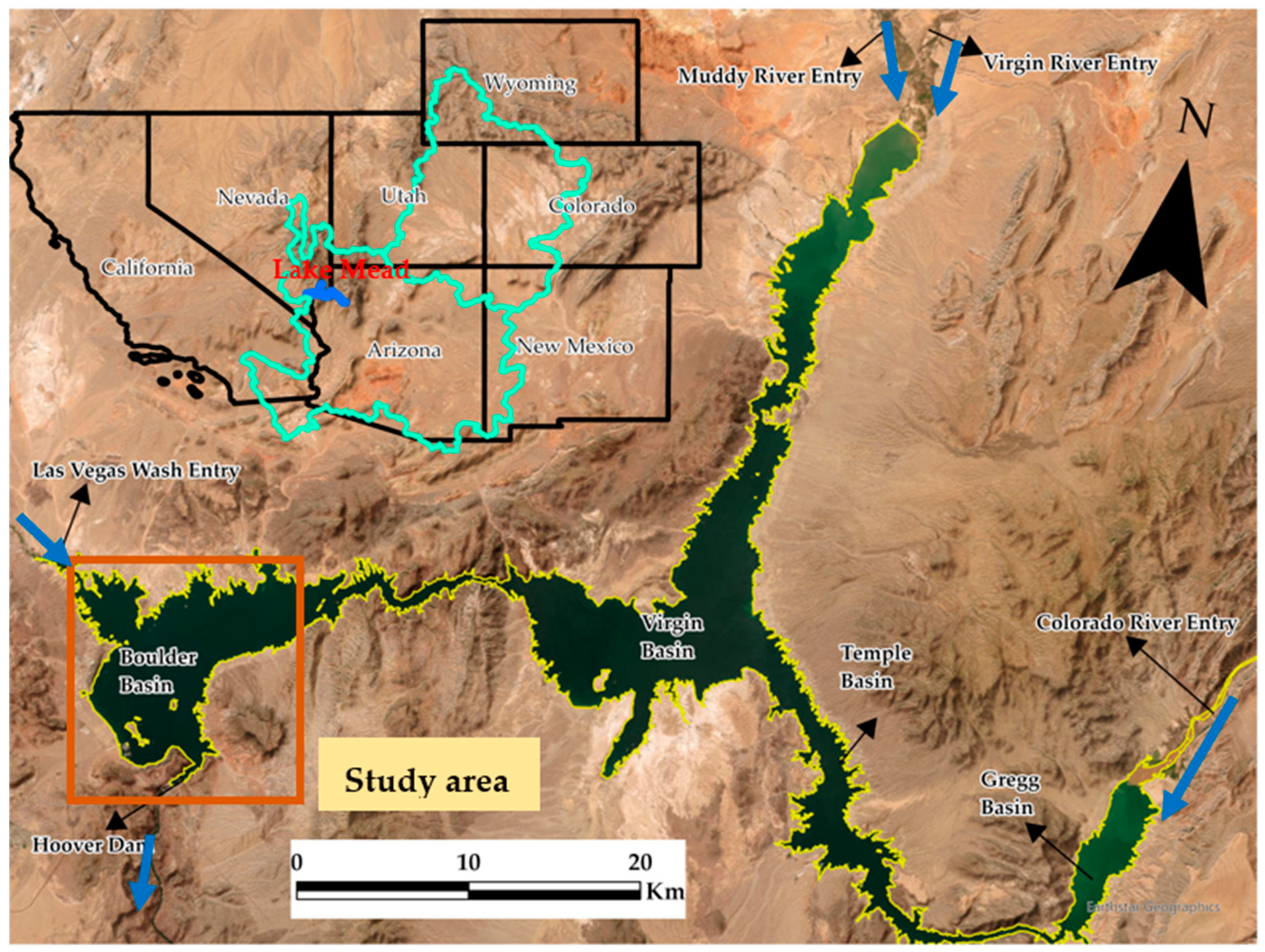
Figure 1. Detailed map of Lake Mead located on the Colorado River Basin (light green boundary). The location of the lake is indicated by the small boundary within the Colorado River Basin and the enlarged as depicted by the yellow boundary. The study area is shown by the orange square. boundary.
Water 15 02439 g001
Figure 2. Detailed map showing stations (marked with red dots and numbers) on Lake Mead. The yellow arrows indicate the flow directions into the study area. The Colorado River through the lake is identified by the blue arrow.
Water 15 02439 g002
Figure 3. Boxplots of the studied WQPs.
Water 15 02439 g003
Figure 4. Correlation matrix for the variables.
Water 15 02439 g004
Figure 5. TDS estimations for the various ML models with the 45° bisector line. LR denotes linear regressors, SVM denotes support vector machine or regressors, KNN denotes K-nearest neighbor regressors, ANN denotes artificial neural network, Random Forest denotes random forest regressor, Gradient Boosting denotes Gradient Boosting Regressor, Bagging denotes bagging regressor, Extra Trees denote extra tree regressors, and XGBoost denotes extreme gradient boosting.
Water 15 02439 g005aWater 15 02439 g005b
Figure 6. Boxplots of the observed and estimated TDS concentration for the various ML models. LR denotes linear regressors, SVM denotes support vector machine or regressors, KNN denotes K-nearest neighbor regressors, ANN denotes artificial neural network, Random Forest denotes random forest regressor, Gradient Boosting denotes Gradient Boosting Regressor, Bagging denotes bagging regressor, Extra Trees denote extra tree regressors, and XGBoost denotes extreme gradient boosting.
Water 15 02439 g006aWater 15 02439 g006b
Figure 7. Identification of the optimal lag time using autocorrelation analysis.
Water 15 02439 g007
Figure 8. Time series plots of the observed and estimated TDS for the ML model.
Water 15 02439 g008aWater 15 02439 g008b
Table 1. Lake Mead sampling stations [55].
No.StationLocationLat. /Long.Sampling Frequency
1LWLVB1.2In channel 1.2 miles from the confluence of the Las Vegas Wash and Las Vegas Bay.MovableWeekly (March–October)
Monthly (November–February)
2LWLVB1.85In channel 1.85 miles from the confluence of the Las Vegas Wash and Las Vegas Bay.MovableWeekly (March–October)
Monthly (November–February)
3LWLVB2.7In channel 2.7 miles from the confluence of the Las Vegas Wash and Las Vegas Bay.MovableBiweekly (March–October)
Monthly (November–February)
4LWLVB3.5In channel 3.5 miles from the confluence of the Las Vegas Wash and Las Vegas Bay.MovableBiweekly (March–October)
Monthly (November–February)
5IPS3In Boulder Basin on the northeast side of the mouth of Las Vegas Bay.36.0896° N 114.7662° WMonthly year-round
6BB3In Boulder Basin on the northeast side of Saddle Island.36.0715° N 114.7832° WMonthly year-round
7CR350.0SE0.55Between Battleship Rock and Burro Point.36.0985° N 114.7257° WMonthly year-round
8CR346.4In Boulder Basin between Sentinel Island and the shoreline of Castle Cove.36.0617° N 114.7392° WMonthly year-round
9CR342.5In Boulder Basin in the middle of Black Canyon, near Hoover Dam.36.01910° N
114.7333° W
Monthly year-round
Table 2. Summary statistics of TDS concentration at sampling locations.
No.StationMax. TDS mg/LAvg. TDS mg/LMin. TDS mg/LStd. TDS mg/LTime Range
1LWLVB1.210307165551072016–2021
2LWLVB1.85957670523752016–2021
3LWLVB2.7803626459512016–2021
4LWLVB3.5784605493412016–2021
5IPS3661581521242017–2021
6BB3789598536332016–2021
7CR350.0SE0.55700585532292016–2021
8CR346.4667588397352016–2021
9CR342.5667588524292016–2021
Table 3. Optimal values of the hyperparameters for the standalone and ensemble models.
ModelHyperparameterOptimal Value
StandaloneLRFit interceptFalse
SVMKernelLinear
C1
Gamma0.1
KNNNumber of neighbors10
WeightsUniform
ANNHidden layer sizes100
ActivationReLU
EnsembleBaggingNumber of estimators20
GBMLearning rate0.1
Number of estimators100
ETNumber of estimators100
RFNumber of estimators100
Maximum depth3
XGBoostLearning rate0.1
Maximum depth3
Table 4. Performance metrics for ML models used in the study.
Training (Sample Size =1928)Testing (Sample Size = 483)External Validation (Unseen Data)
(Sample Size = 553)
ModelR2RMSE (mg/L)MAE (mg/L)PMARE (%)SINSEPBIAS (%)R2RMSE (mg/L)MAE (mg/L)PMARE (%)SINSEPBIAS (%)R2RMSE (mg/L)MAE (mg/L)PMARE (%)SINSEPBIAS (%)
LR0.8034.7720.403.060.050.80−0.250.8334.2820.183.040.050.83−0.090.8233.0918.722.870.050.820.11
SVM0.8035.3519.502.900.060.800.400.8334.6119.012.830.050.830.620.8134.4018.862.870.050.810.97
KNN0.8431.7619.212.880.050.84−0.230.8136.9822.513.380.060.81−0.070.8035.1221.183.240.060.800.09
ANN0.8034.8220.183.030.050.80−0.270.8334.3519.702.950.050.830.060.8233.3318.802.880.050.820.09
Bagging0.9714.578.471.270.020.97−0.110.8136.4122.673.420.060.81−0.060.7836.6822.193.390.060.78−0.03
GBM0.8728.0817.282.610.040.87−0.190.870.8433.8820.143.020.050.840.8134.5220.713.190.060.810.02
ET1.002.280.140.020.001.000.000.8037.3522.673.420.060.80−0.080.7737.6822.263.400.060.770.06
RF0.8233.7020.443.070.050.82−0.280.8136.8421.793.240.060.810.060.8035.2522.133.420.060.80−0.30
XGBoost0.8728.8717.542.640.050.87−0.200.8433.9820.193.020.050.840.080.8134.1920.513.160.050.81−0.01
Table 5. Summary of the performance ranks for the ML models.
Training (Sample Size =1928)Testing (Sample Size = 483)External Validation (Unseen Data)
(Sample Size = 553)
OverallAvg.
RanksRanksRanks
ModelR2RMSEMAEPMARESINSEPBIASAvg.R2RMSEMAEPMARESINSEPBIASAvg.R2RMSEMAEPMARESINSEPBIASAvg.
LR77887767.133454384.311121172.04.5
SVM99669998.155113594.144313494.05.4
KNN55555555.088778857.366666655.96.0
ANN88778877.644225423.322232262.74.5
Bagging22222222.066886636.188878837.15.1
GBM33333333.011341111.755555524.63.1
ET11111111.099999978.799989948.16.0
RF66996687.177667746.377797787.47.0
XGBoost44444444.022532263.133444313.13.4
Disclaimer/Publisher’s Note: The statements, opinions and data contained in all publications are solely those of the individual author(s) and contributor(s) and not of MDPI and/or the editor(s). MDPI and/or the editor(s) disclaim responsibility for any injury to people or property resulting from any ideas, methods, instructions or products referred to in the content.