Article

Estimating Evapotranspiration from Commonly Occurring Urban Plant Species Using Porometry and Canopy Stomatal Conductance

by
Syed Hamza Askari
*,
Simon De-Ville
,
Elizabeth Abigail Hathway
and
Virginia Stovin
Department of Civil & Structural Engineering, The University of Sheffield, Sir Frederick Mappin Building, Mappin Street, Sheffield S1 3JD, UK
*
Author to whom correspondence should be addressed.
Water 2021, 13(16), 2262; https://doi.org/10.3390/w13162262
Submission received: 28 June 2021 / Revised: 9 August 2021 / Accepted: 16 August 2021 / Published: 19 August 2021

Abstract

:
Evapotranspiration (ET) is a key moisture flux in both the urban stormwater management and the urban energy budgets. While there are established methods for estimating ET for agricultural crops, relatively little is known about ET rates associated with plants in urban Green Infrastructure settings. The aim of this study was to evaluate the feasibility of using porometry to estimate ET rates. Porometry provides an instantaneous measurement of leaf stomatal conductance. There are two challenges when estimating ET from porometry: converting from leaf stomatal conductance to leaf ET and scaling from leaf ET to canopy ET. Novel approaches to both challenges are proposed here. ET was measured from three commonly occurring urban plant species (Sedum spectabile, Bergenia cordifolia and Primula vulgaris) using a direct mass loss method. This data was used to evaluate the estimates made from porometry in a preliminary study (Sheffield, UK). The Porometry data captured expected trends in ET, with clear differences between the plant species and the reproducible decreasing rates of ET in response to reductions in soil moisture content.

1. Introduction

Cities are dominated by impervious surfaces, which lead to high volumes and rates of surface water flow following rainfall [1]. Stormwater runoff contributes to urban flooding and poor urban water quality [2]. At the same time, hard impervious surfaces (often dark in colour) and a lack of moisture (because of reduced vegetation coverage) also contribute to the Urban Heat Island (UHI) [3] associated with tall buildings and their reflective surfaces trapping incoming solar radiation. The UHI creates an added perturbation alongside global warming [3].
Internationally it is now recognised that urban resilience to climate change can be supported by the adoption of stormwater management techniques that aim to mimic the natural hydrological cycle, often using vegetated systems designed to encourage evapotranspiration. Within England, these approaches are referred to as Sustainable Drainage Systems (SuDS) [2]. SuDS are designed to efficiently manage the drainage of surface water in the urban environment by infiltrating, storing or re-using it at source. Examples include vegetated devices such as green roofs, rain gardens, swales and street trees [4]. Implementing SuDS enhances evapotranspiration (ET) within the urban hydrological cycle. This leads to a reduction in the volumes/rates of surface water flow and to a mitigation of urban heat stress through the absorption of incoming radiation by green surfaces [5,6].
ET is defined as water transpiring through pores and evaporating from the surfaces of green foliage, vegetation, growing plants and planting media surfaces (where there is not 100% coverage) [7]. Green surfaces intercept and retain rainfall, subsequently releasing water back into the atmosphere before it has a chance to enter drainage networks. ET restores the stormwater retention capacity of a city. In the process, it also uses incoming solar radiation to produce a latent heat flux (during evapotranspiration), thereby reducing temperature in the urban area [8].
For local authorities to implement SuDS and Green Infrastructure (GI) on a large scale, evidence that they will perform effectively is required. Stormwater engineers typically utilise hydrological/hydraulic models to estimate the impact that specific design interventions will have on downstream flood risk and on receiving water quality. Such models therefore need to properly capture all relevant hydrological processes. The amount of surface runoff generated by a rainfall event is dependent on the retention capacity of a SuDS device. Retention capacity (or initial losses) depends on moisture levels within the substrate, which are controlled by ET rates during the antecedent dry period [9]. In the context of green roof hydrological modelling, for example, Stovin et al. [10] proposed an approach to modelling ET as part of a validated rainfall-runoff model. Their work showed that ET can account for up to 50% of the annual water budget for a green roof. Stovin et al. [10] and Berretta et al. [11] both found that moisture loss rates (from GI) due to ET have an exponential decay in dry periods.
While there are established methods for estimating ET for agricultural crops [12], relatively little is known about ET rates associated with plants in urban Green Infrastructure settings. Compared with green roofs, many SuDS (e.g., roadside bioretention cells) incorporate trees and larger plants, for which ET estimates are not available. Attempts to quantify ET to date have focused on invasive, infrastructure heavy techniques, such as lysimetry and chamber methods [13]. Lysimetry is a water balance approach, in which incoming and outgoing moisture flows from a sample volume are monitored to estimate ET. Chamber methods enclose vegetation in a temporary environment to monitor changes in the local humidity due to ET [14]. These techniques provide useful data in controlled research experiments but cannot readily be transferred to field measurements in urban Green Infrastructure settings. Data are required from real field settings to understand how different plant assemblages and urban microclimates affect ET rates.
Shuttleworth [15,16] provides a comprehensive list of possible ET measurement methods. Of these methods, porometry appears to be potentially applicable in this context. Porometry is a characterisation technique based on the diffusion of water from leaf stomata. The technique measures leaf stomatal conductance through changes in humidity caused by a displacement of water from inside the stomatal cavity [17]. Stomatal conductance is defined as the rate of water vapour exiting the stomata (stomata are small pores or openings that are apparent on plants) [18]. It is an inherent physical property of a plant, providing an indication of the degree of the stomatal opening of a leaf. However, leaf stomatal conductance is not enough to make an estimation of ET; it does not provide specific information about the quantity of water leaving the stomata. The authors have been unable to find any published work that has used data directly from porometry to estimate ET. There are two challenges when estimating ET from porometry: converting from leaf stomatal conductance to leaf ET and scaling from leaf ET to canopy ET. Spinelli et al. [19] and Zhao et al. [20] have both provided relationships linking ET to canopy-scale stomatal resistance (the inverse of stomatal conductance). Spinelli et al. [19] also outlined a method to convert leaf stomatal resistance to canopy stomatal resistance, based on whether leaves were sunlight exposed or shaded.
The research aim is to investigate the feasibility of using Porometry to estimate ET from commonly occurring urban plants. There are two key research objectives: a method to transfer between the measurements of leaf stomatal conductance to leaf ET and the scaling of leaf ET to canopy ET.

2. Materials and Methods

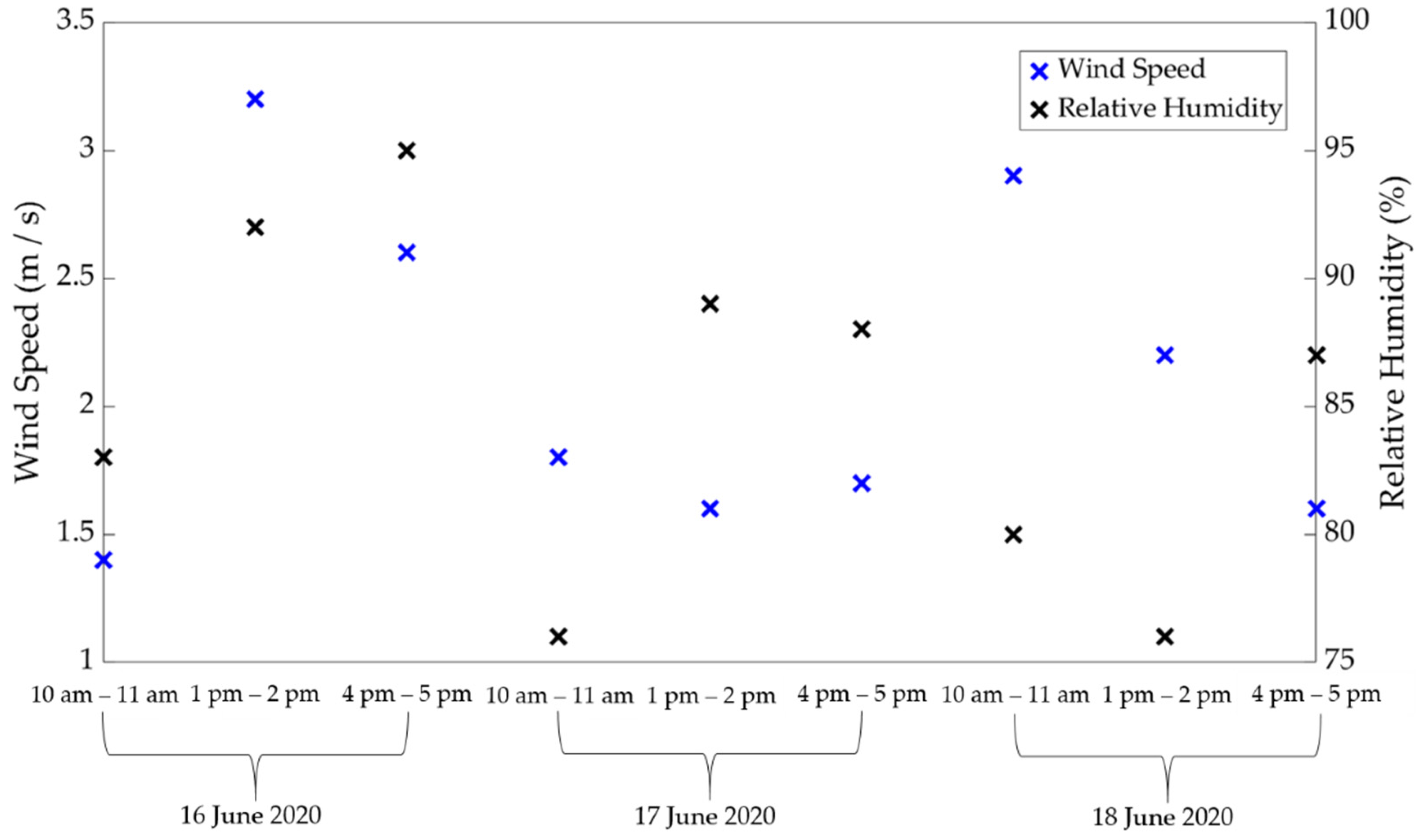
2.1. Materials and Location

This experiment aimed to estimate ET from three commonly occurring urban plant species that would be found in green infrastructure such as green roofs and rain gardens. The experiment took place in the suburban garden environment setting of Crookes, North West Sheffield, UK (53.3860, −1.5046) at an altitude of 208 m. The experiment took place outdoors so that a natural relationship between plant ET and the local microclimate could be explored. The three plants chosen for this investigation were: Sedum spectabile, Bergenia cordfolia and Primula vulgaris (Figure 1). These plants were chosen because they are often found in urban landscape planting, including SuDS/Green Infrastructure, and because they were expected to demonstrate contrasting rates of ET (Table 1).

2.2. Obtaining ET from Mass Losses

Measurements of ET rates from each potted plant based on mass losses serve as a reference for the estimations of ET made via porometry from the same plants. The potted plant was considered a closed system in which mass losses are only a result of ET and mass gains only arise from controlled irrigation. Plant pots were brought indoors on rainy days to avoid unknown inputs of moisture. Changes in plant biomass can also affect system mass; regular photos were taken to account for this. Over a defined period, ET losses from a plant/soil system can be defined as the difference between incoming precipitation, P and irrigation, I and outgoing runoff, R and change in soil moisture content, ∆S over that time, as shown in Equation (1) [21].
E T = P + I R Δ S
The experiment ran over a 3-day period from 16–18 June 2020. A 3-day period was chosen to provide an opportunity to observe actual ET rates decay exponentially in response to reduced soil moisture content, whilst not allowing for the growing media to reach its Permanent Wilting Point (PWP).
At the start of each measurement period, each plant’s soil moisture content was at, or close to, its field capacity (θfc). Field capacity defines the condition when the soil can hold no more moisture under gravity after excess water has been drained from the macro-pores, i.e., not held in place by capillary action or hydrostatic forces. Each plant pot was placed in a bucket and irrigated by slowly filling the bucket with water up to the lip of the plant pot. This was done to bring the soil to saturation. After irrigation, the pots were placed on a drainage board over a collection vessel and allowed to drain for up to 2 h. The collection vessel was used to record the volume of water that had drained through the soil. The volume of drainage was recorded at 10-min intervals. When the collection vessel had recorded no change in drained water for 30 min, the plant pots were assumed to have reached field capacity and were placed on a balance and their mass recorded. It is not essential to be exactly at field capacity, but this method ensures that the plants will be close to θfc and therefore provides information about plant ET in plentiful moisture conditions. The method adopted here is comparable with the standard method recommended by the FLL for determining the maximum moisture holding capacity (field capacity) in green roof substrates [22]. In the subsequent days after irrigation, it may also be possible to observe ET effects in moderately moisture stressed conditions.
The irrigation process was completed by 10:00 a.m. on the first day of investigation. The mass of each plant pot was then recorded at 10:00 a.m., 1:00 p.m., 4:00 p.m. and 7:00 p.m. on that day and each subsequent day for three days. This allowed ET rates to be evaluated for three, 3-h periods each day. The mass changes in grams were converted into a volume in millilitres by assuming that the density of water is 1000 kg·m−3. Volumes were converted into depths of moisture change due to ET, in mm, by assuming that the mass loss occurred over the complete canopy one-sided leaf surface area of each plant. The recorded 3-h ET rate was divided by three to give an ET rate in mm·h−1.
The leaf canopy surface area of each plant was calculated using five representative leaves (from each plant) to find average leaf widths/lengths. The width and length of each representative leaf was measured and used to find an average leaf width/length for each plant. Assuming each leaf was rectangular, an assumed typical leaf area for each plant was calculated. The typical leaf area was multiplied by the number of leaves in each canopy to find the complete leaf surface area of each plant. The calculated total leaf surface areas for the S. spectabile, B. cordfolia and P. vulgaris species were 0.0546 m2, 0.0448 m2 and 0.0756 m2, respectively.

2.3. Using Porometry to Obtain Canopy Stomatal Conductance and ET

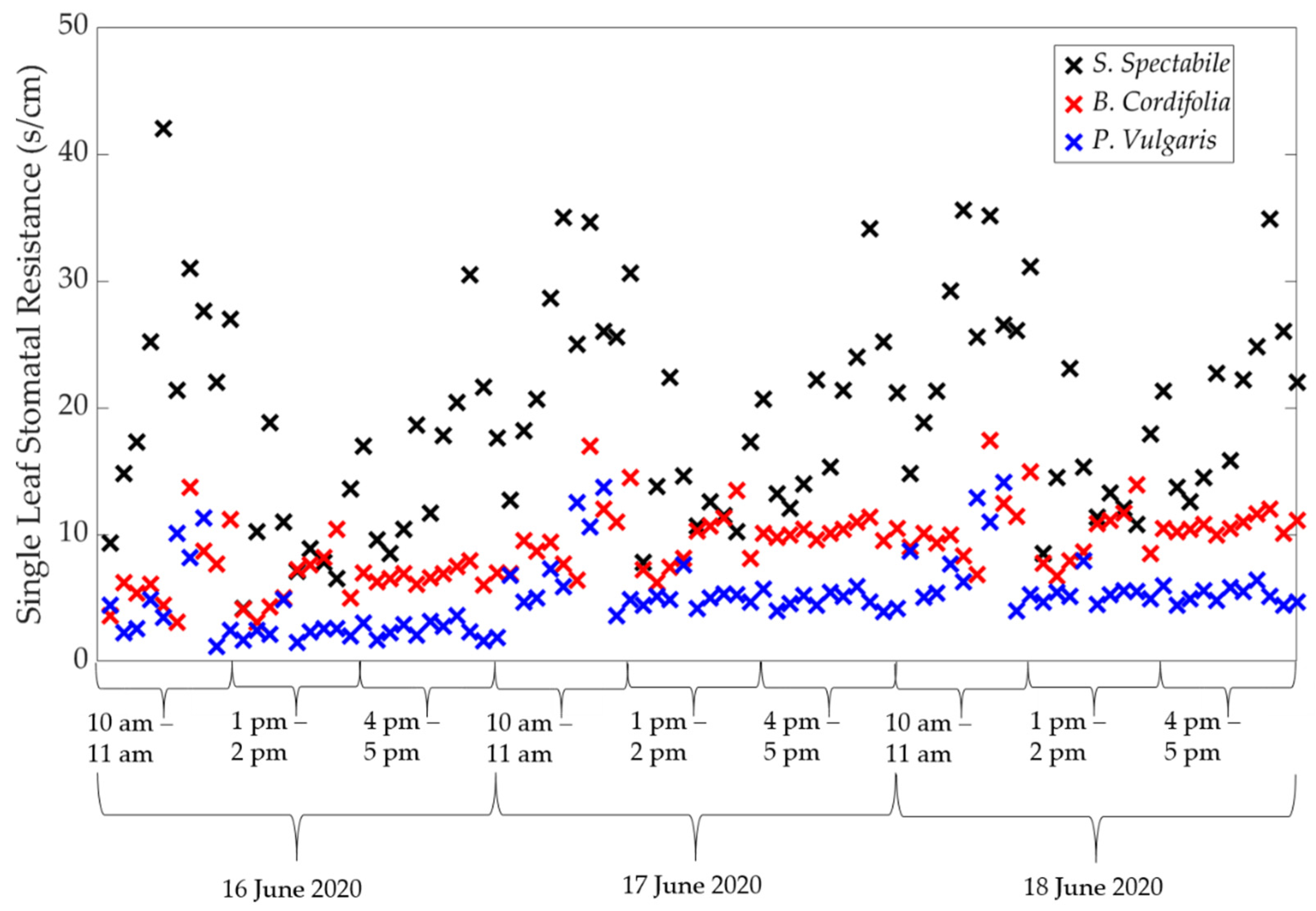
2.3.1. The Porometer

An AP4-Porometer (Delta-T Devices, Cambridge, UK) was used to obtain ET rates from the three plant pots. Porometry is a hands-on technique that uses a porometer to directly measure gaseous mass transfer through a plant’s stomata. It does this by recording stomatal conductance or resistance through the leaf of a plant [23]. All plants produce most of their transpiration from leaves, and this is why the measurements are concentrated here [18]. The porometer is a compact handheld device. The porometer creates a temporary chamber environment enclosing part of a leaf. The device measures the time elapsed for a section of the leaf to release a sufficient amount of water vapour to change the relative humidity inside the chamber by a fixed amount [18]. This value is directly compared to a prepared calibration plate of known resistance/conductance.
When the chamber’s relative humidity increases to a system-defined set point, dry air is pumped into and circulated within the chamber. The porometer records the time to produce the change in relative humidity, and measurements are repeated until a constant time elapsed for the same relative humidity rise is established [24]. This provides the basis of the stomatal conductance or resistance measurements, which are computed by the device in units of m·s−1 or s·m−1, respectively.
Once a dataset of leaf stomatal conductance has been recorded, the results are used to calculate representative ET rates. This is done using a method to scale measurements from the single-leaf to canopy level in combination with climatic measurements.

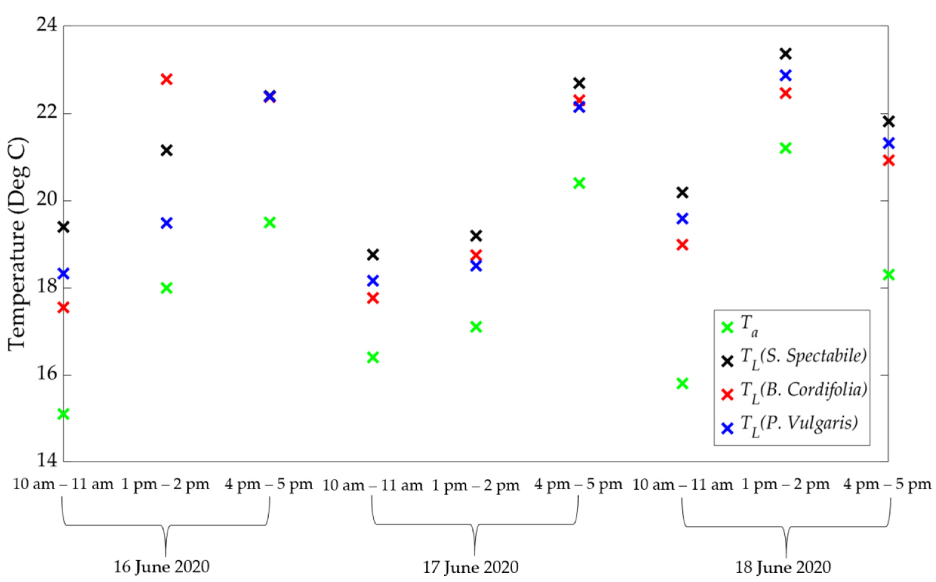
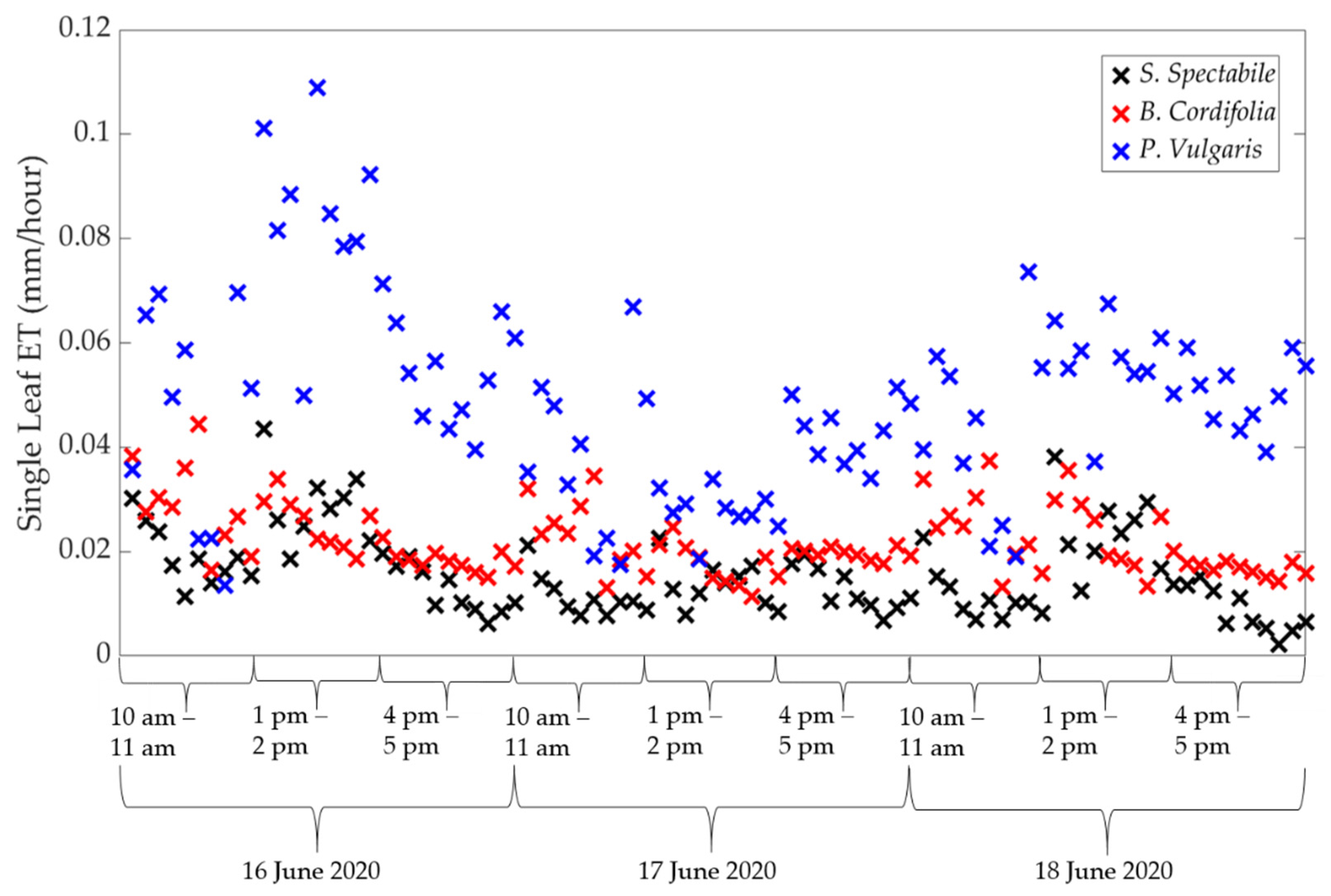
2.3.2. Calculating Single Leaf ET

ET is typically estimated on the scale of a vegetated canopy or larger. Attempting to quantify ET on the leaf scale is not an approach typically found in the literature. The studies highlighted in the introduction [19,20] explored ET on vegetated canopies, tens of metres in size. This study attempts to quantify ET in a novel way by quantifying the physiological properties on the leaf scale and working upwards to a complete definition of the canopy.
ET is a result of a close relationship between the physiological properties of a plant (the size and diffusivity of stomata) and the local micrometeorological properties. To use porometry to estimate ET, local estimations of leaf temperature, air temperature, relative humidity and wind speed are required. ET is the diffusion of water vapour between two mediums, from within the stomata to the immediate local air layer [25]. Fick’s law of diffusion states that the rate of diffusion is dependent on the gradient of concentration between the two mediums [26]. The local climate measurements are used to estimate a difference in water vapour concentration between inside the stomata and the adjacent air layer [27]. ET [m·s−1] is calculated via a difference in water vapour concentrations (Equation (2)).
E T = g s g a g s + g a ( C s C a )
where gs [m·s−1] describes leaf stomatal conductance measured using the porometer, ga [m·s−1] is the air boundary layer conductance and Cs [%] and Ca [%] are the concentration of water vapour within the stomata and air layer, respectively. gs and ga describe the resistance to movement experienced by water vapour molecules from inside the leaf to the bulk air. ga is a function of wind speed, u [m·s−1] and the characteristic dimension of leaf width, d [m], as shown in Equation (3) [26].
g a = 0.135 u 0.72 d
The concentration of water vapour is a function of the saturation vapour pressure at local temperature, es(T) [Pa], and air pressure, P [Pa]. Air pressure can be found as a function of local altitude [26]. For concentration at the stomata level, leaf temperature, TL [°C], is used, and for within the boundary layer, air temperature, Ta [°C], is used. The concentration of water vapour in the air boundary layer is also a function of the local relative humidity, hr [%]. Concentration calculations are described by Equations (4)–(6) [26].
C s = e s ( T L )   P  
C a = e s ( T a ) h r P  
e s ( T ) = 0.611   e x p ( 17.5   T 240.97 + T )
The specific formulation of saturation vapour pressure outlined in Equation (6) was chosen, as it describes vapour pressure resulting from changes in state (liquid to gas from inside to outside the leaf).
Data on leaf stomatal conductance and leaf temperature were obtained directly from the porometer. This investigation was completed as a home study during a National UK lockdown for the COVID-19 pandemic, and on-site climate measurements were not possible due restricted equipment access. The air temperature, relative humidity and wind speed data were provided by a nearby weather station as part of the Urban Flows Observatory network [28], situated 269 m away from, and at an elevated height of 15 m above, the test site. The conditions measured by the weather station were assumed equal to those at the test site during the investigation. The climate data were only available at an hourly temporal resolution, so values were assumed constant for each stomatal measurement in a single hourly period. This approach might not capture the changing interactions that are occurring temporally across the entire canopy surface between each leaf/stomatal cavity and the immediate air layer.

2.3.3. Scaling Single Leaf ET to Canopy ET

The process of converting single leaf ET to pot ET does not follow a standardised method. The objective is to use an appropriate method to obtain a mean value of leaf ET, weighted by a Leaf Area Index (LAI). LAI is a non-dimensional representation of the total one-sided area of leaf tissue per unit ground area of a vegetated canopy [29]. In making the transition to pot level ET, ET from different types of leaves was considered. These were grouped into ET from sunlight exposed leaves, shaded leaves, young leaves, old leaves, middle aged leaves and ET from the upper and lower surfaces of leaves. Based on the scaling methods identified in the literature [30,31,32], Equation (7) describes an original approach to scale between the leaf and canopy level. This builds on the work of Spinelli et al. [19], where leaves were only categorised by sun or shade. Investigations with the porometer have shown that leaf properties differ depending on their age and from which side of the leaf they transpire. These variables have been accounted for in this proposed formulation for canopy ET.
E T c a n o p y = i a l l   l e a f   t y p e s L A I i   ( E T ¯ u i + E T ¯ l i )  
In Equation (7), canopy ET is found by summing the LAI of each leaf type multiplied by the sum of the average ET from the upper, E T ¯ u i , and lower, E T ¯ l i , leaf surfaces (again, for each leaf type). The sum over i leaf types considers six different groups: sunlight exposed leaves that are young, middle-aged or old and shaded leaves that are young, middle-aged or old. During this investigation, no part of any plant pot was in the shade in any measurement session. Therefore, only the first three terms (sunlight exposed) were relevant in the analysis. The three shaded terms will be important for future studies on a larger vegetated canopy.
The leaf area index for each group was found using a ratio between the leaf surface area of each type (young, old and middle aged) and the pot surface area. Counting the number of leaves in each group by eye, the fraction of surface area for each leaf type was found from the calculations of the total leaf surface area described in the mass-loss method calculations in Section 2.1. The one-sided surface area of each leaf type (from each plant) was then divided by the relevant pot surface area to find the leaf area index values presented in Table 2.
The start of each porometer measurement session coincided with the mass measurement of each plant pot. Each stomatal measurement session took place between 10:00–11:00 a.m., 1:00–2:00 p.m. and 4:00–5:00 p.m. (each day). This gives the pot level canopy ET at these hourly periods. The mass loss method provided the ET rates from each plant for 3-h periods between 10:00 a.m.–1:00 p.m., 1:00–4:00 p.m. and 4:00–7:00 p.m. ET rates are expected to vary during the day. These three time periods were chosen to discern whether porometry could capture this daily variation.

3. Results and Discussion

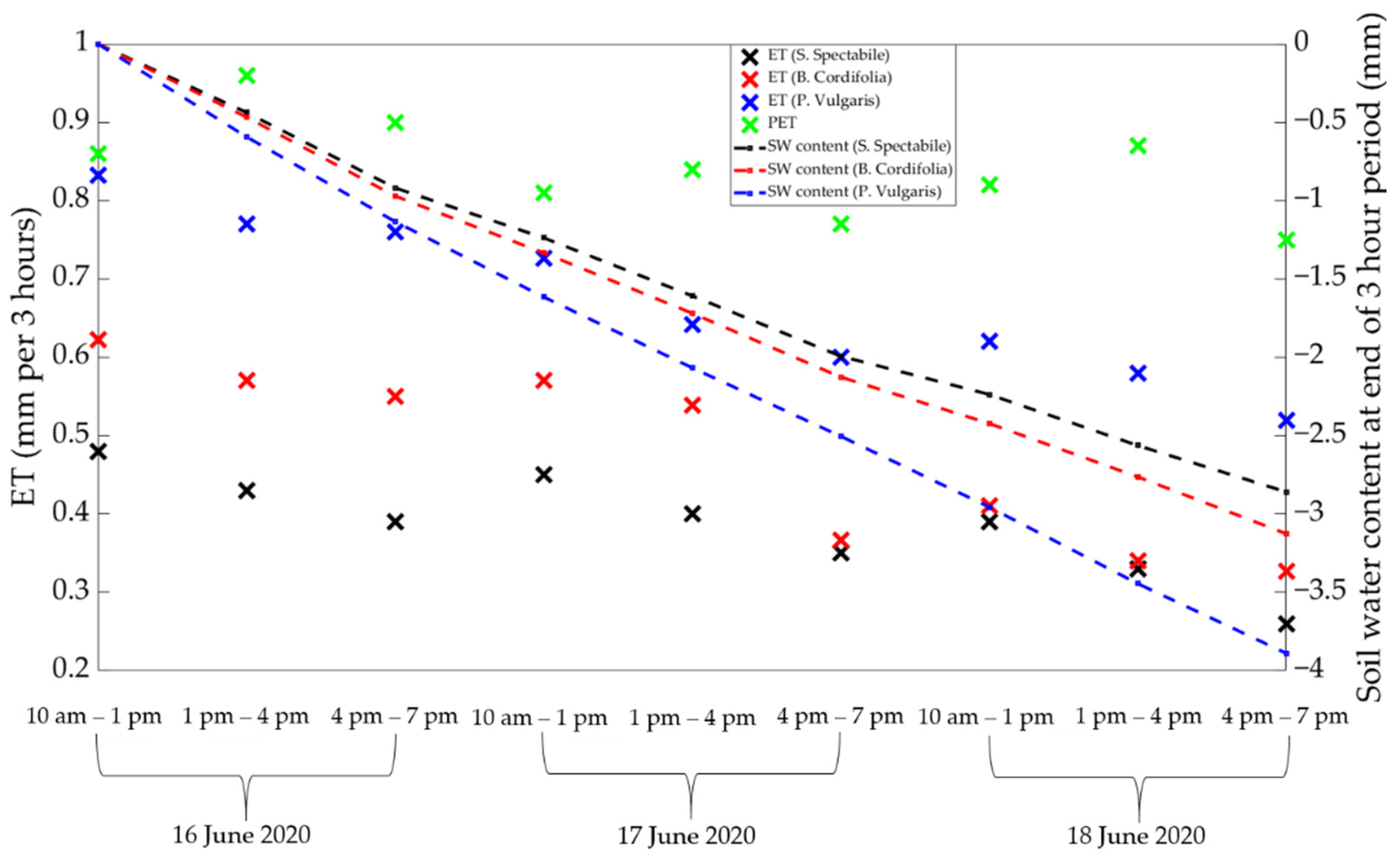
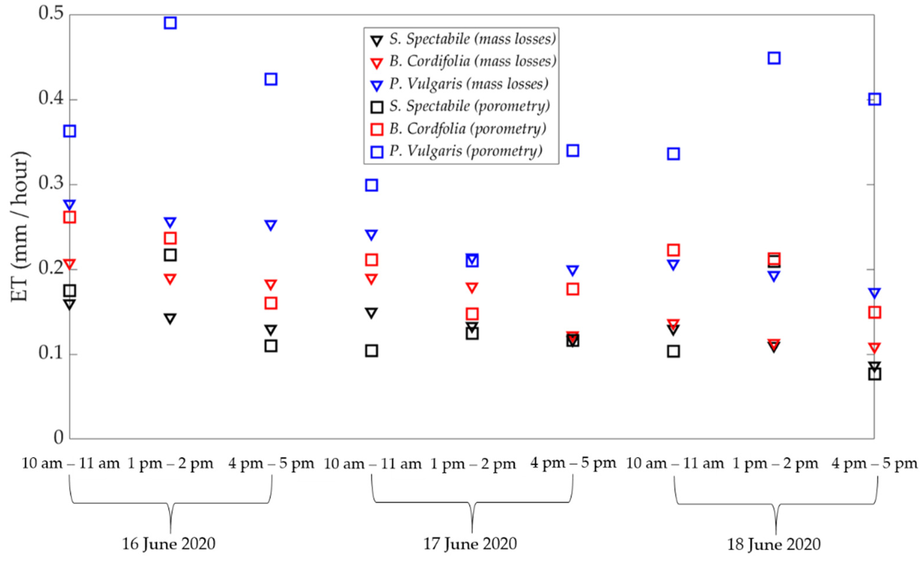
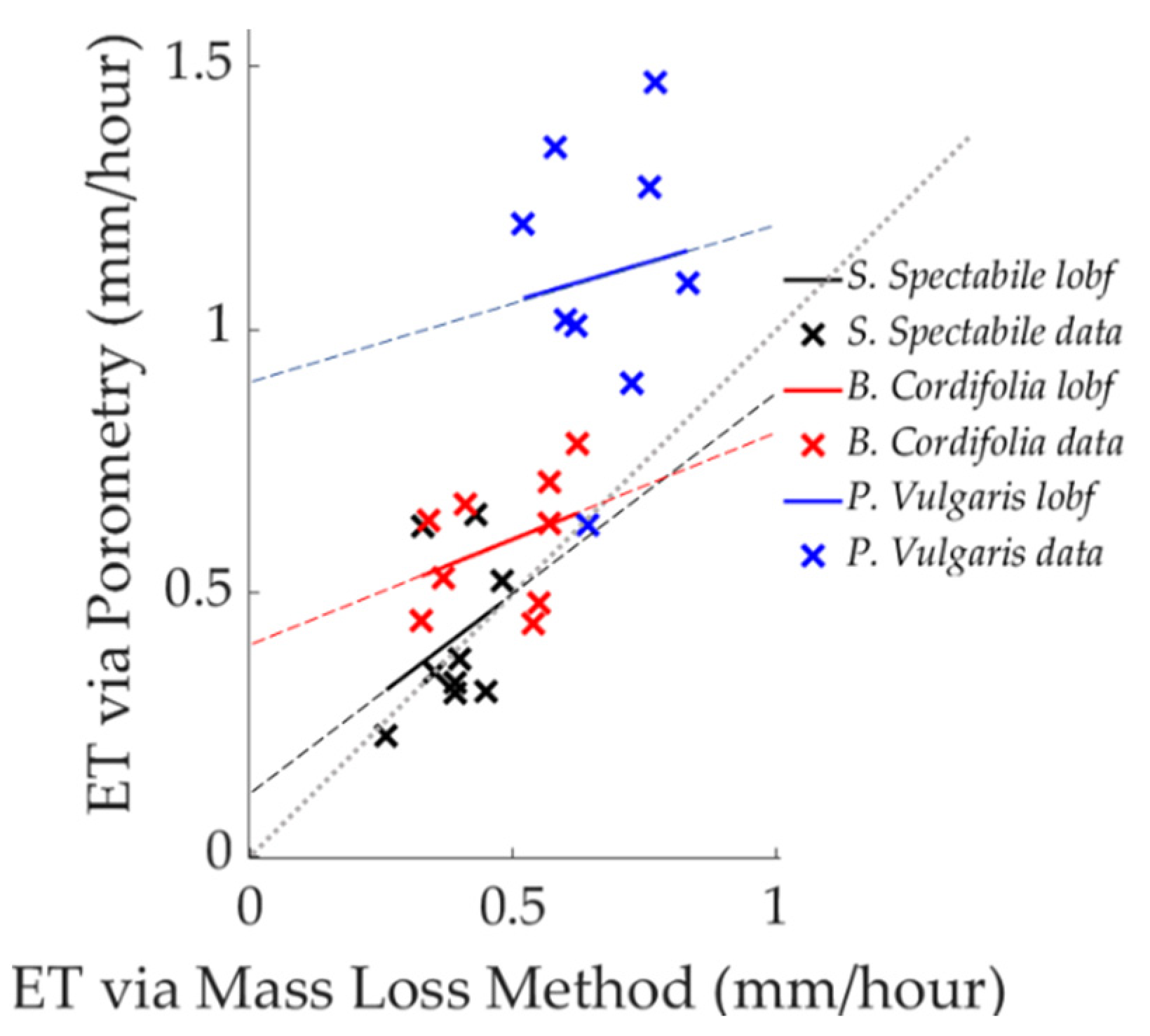
3.1. Comparison of Estimated ET between Porometric and Mass-Loss Measurements

The porometer recorded values of leaf stomatal resistance, rs [s·m−1]; this is the inverse of leaf stomatal conductance, gs [33].
r s = 1 g s
The single leaf stomatal conductance data from each of the three plants from the porometer are shown in Figure 2. Eight leaves from each plant were used to sample representative stomatal resistance: four middle-aged leaves, two young leaves and two old leaves. Four middle-aged leaves were used in the sample (compared with two young and old leaves), as each plant canopy was dominated by this leaf type. A larger sample of middle-aged leaves provides a better representation of the canopy. One measurement of the stomatal resistance from each leaf was taken in each session.
Old-aged leaves recorded stomatal resistance values higher than middle-aged and young leaves. This implies that, comparatively, old-aged leaves do not significantly contribute towards canopy ET rates. The sampled data suggest that young leaves have similar rates of stomatal resistance to middle-aged leaves.
Figure 2 shows the S. spectabile leaves to have highest stomatal resistance and P. vulgaris leaves the lowest. There is greater restriction to water flow out of leaf stomata with greater resistance. Therefore, expected lower rates of ET (and vice versa) were demonstrated via Equation (2). A high rs describes a low concentration of water vapour within the stomatal cavity. Sedum spectabile leaves are shown to have high rs, which is also shown in the literature [34].
Figure 3 presents the hourly air and leaf temperature data, while Figure 4 presents the windspeed and relative humidity. The data in Figure 2, Figure 3 and Figure 4 were used to estimate single leaf ET in each measurement session, with Equations (2)–(6); the results are shown in Figure 5.
The data in Figure 5 corroborate the resistance data in Figure 2; S. spectabile has the lowest ET rates. The single leaf ET data also highlight a degree of regular diurnal variation over the 3-day period, peaking at 1:00–2:00 pm, which is to be expected. There is a noticeable increase in ET rates on day three compared with day two; this could be a result of an increase in temperatures (see Figure 3).
Canopy ET (pot level) was calculated for each hour using the model described in Equation (7). Nine values of canopy ET (three each day for three days) were calculated for each plant. The estimates found using the mass loss method are compared with the ET results from porometry in Figure 6. The comparisons are very encouraging; the basic physiological processes of a plant system undergoing losses via ET are highlighted in the data. Similar trends and variations over the 3-day period are observed, and it is encouraging to find that porometry can distinguish ET rates between different plants, confirming that S. spectabile plants have the lowest ET rates, with P. vulgaris having the highest.
It would be expected to find the highest ET levels in the middle of the day when there is greater exposure to the sun’s solar radiation [35]. This is only evident in the porometry data for S. spectabile. The results in Figure 6 are scattered with respect to time of day. This is not surprising for three days of data, as the interacting effects of temperature, radiation, wind and humidity could be very different with time. A larger dataset in a further study will be required to confirm these diurnal trends from all plants.
Figure 6 shows that porometry typically overestimates ET compared to the reference mass loss data. The average percentage difference is 43.3% (considering all three plants). There is scope for further work based on these initial findings. The methodology is able to capture some of the underpinning processes, even though many assumptions have been used.
In Figure 6, when both methods show similar results in a particular measurement session, this occurs for all plants. When results from both methods diverge in a particular session, they seem to diverge for all plants; this divergence could pertain to another consistent factor affecting the plant systems.
Figure 7 provides a direct comparison between the porometric estimates of ET and the baseline mass loss data. Sedum spectabile and B. cordfolia suggest a closer relationship between both sets of data than P. vulgaris. Sedum spectabile shows the strongest relationship between both sets of data; the line of best fit (lobf) almost extrapolates to the origin. The reason for this may be due to S. spectabile’s low ET rates in comparison to those of P. vulgaris. The level of scatter in the plots also highlights the variability in the data and provides reason for further study.

3.2. Uncertainty in Analysis

Understanding where the uncertainty lies requires consideration of the relationship between boundary/stomatal conductance, climatic factors and the resulting impact on ET.
One source of uncertainty is that exact measurements of the local climatic conditions (where the system is placed) have not been used. This does not take into account the effects of local microclimate. The yard space where this experiment took place is sheltered by tall buildings. Therefore, shading effects will have an impact on the air temperature. This would result in lowered ET rates, which correlates with the findings in Figure 7; porometric estimated ET is mostly overestimated.
Considering Equation (2), it is shown that this methodology is dominated by ET’s sensitivity to temperature (leaf and air). Equation (5) shows that ET is dependent on the exponent of temperature, whereas a linear relationship with relative humidity is found. This highlights that small discrepancies in temperature can have large impacts on the final calculations of ET, further signifying the importance of accurate temperature readings. Leaf temperature is provided by the porometer, highlighting that the uncertainty in the final results is most likely from the error in the air temperature readings.
Local wind speed is also affected by surrounding microclimate effects. Boundary layer conductance, and hence ET, have a positive proportionality with wind speed. ga is a function of the square root of wind speed, producing an exponential functionality. Due to the sheltered nature of the test site, wind speed measurements from the weather station will result in an over-estimation of ET. There is a high sensitivity to potentially non-representative readings of wind speed.
Characteristic leaf width is another variable that has an exponent relationship with boundary layer conductance and ET. In this analysis, a single average characteristic leaf width was used in the calculation for each plant. Each plant system has been viewed as having one type of interaction with the local atmosphere based on a single geometrical leaf size. An uncertainty regarding the final ET results has arisen by disregarding the individual relationship between each leaf and the local air layer. This is encapsulated by the exponent dependency on characteristic leaf width.

3.3. Considering Potential Evapotranspiration (PET) to Understand Decaying ET Rates

Figure 6 shows that ET rates decrease over three days. This is expected in a plant system with falling moisture content in the soil over the same period. Naturally, with lowered moisture content levels, there is less water to draw up through the plant during transpiration. However, it is important to verify whether this effect is starting to dominate the plant system over the duration of the three days. Lowered ET rates can also be influenced by climate conditions; the level to which the local microclimate is having an impact is found through estimating potential evapotranspiration (PET) across the three days. The formula for calculating PET is given by the FAO56 Penman-Monteith (FAO56PM) equation, as shown in Equation (9) [12].
E T = 0.408 Δ ( R n G ) + γ 900 T + 273 u 2 ( e s e a ) Δ + γ ( 1 + 0.34 u 2 )
where PET is potential ET [mm·day−1], Rn is net radiation [MJ·m−2·day−1], G is soil heat flux density [MJ·m−2·day−1], T is mean temperature [°C], u2 is wind speed [m·s−1], es is saturation vapour pressure [kPa], ea is actual vapour pressure [kPa], ∆ is the slope of the vapour pressure curve [kPa·°C−1] and γ is the psychrometric constant [kPa·°C−1]. The soil heat flux is assumed to be zero for this analysis.
PET is a reference value for ET from a common grass species and is only dependent on climatic variables [36]. es and ea are functions of both temperature and relative humidity, both of which have been recorded during the experiment, as well as wind speed. Equation (9) is recommended to be used for daily estimations of PET. However, for this analysis, it is assumed that this formulation of PET remains true for hourly estimations.
The values of PET for each 3-h period are shown in Figure 8 alongside ET rates (mass-loss method) and soil water content decrease (converted from grams to mm) at the end of each 3-h investigation period for each species. ET values here are shown for 3-h periods, in Figure 8, as this was the sampling rate for ET via the mass loss method and the measurements of soil water content. Figure 8 shows that there is a small decrease in PET between the start and end of the investigation. During the same period, soil water (SW) content gradually declines for each plant. Figure 8 highlights that P. vulgaris soil water content decreases at a faster rate than the other two plants, due to the greater ET losses for P. vulgaris (also shown in Figure 8). The evolution of PET and SW over time provides insight into why ET rates have fallen. On day 3, PET marginally rises at the beginning of the day, while ET rates seem to fall compared to the previous day. In this case, actual ET is controlled more by soil water content than by local climate conditions. There is a divergence of ET from PET as moisture becomes limited.
The ET results from the mass loss method are consistently lower than the PET results. This could be a consequence of the shady yard in which the investigations were carried out. The PET estimates are based on data from weather station sensors not located in shade. Another possible reason for the divergence is that the reference crop used for PET estimates is not physiologically similar to the plants used in this investigation. Porometry provides an opportunity to discern crop factors for the trialled plants here or in another study.
There are two steps in the Porometry method: defining ET at the leaf scale and scaling to canopy level. The climate data are used in the prior step. The climate data required for ET estimates are also used in the PET calculations. There is confidence that the raw climate data can provide reliable single leaf ET rates given that ET (from all plants) and PET are both of similar orders of magnitude. This suggests that errors in the Porometry ET data could pertain to issues with the scaling method proposed or with how the physiological properties of the plant have been defined. A further investigation could explore a sensitivity analysis that describes how ET is affected by differing methods of canopy scaling. In Spinelli et al. [13] there was a disparity between scaled stomatal conductance and the results found using the trusted eddy co-variance method. The results in Spinelli et al. [13] suggest there is an issue with the scaling method, which only consider leaves that are shaded or in direct sunlight. This highlights the importance of finding a reliable scaling method that captures variations in a plant canopy.

4. Conclusions

This investigation has demonstrated that it was possible to make reasonable estimations of ET from raw measurements of stomatal conductance made via porometry. This is only achievable with concurrent measurements of local climatic parameters. A clear understanding of the moisture flux near the stomatal cavity (of each leaf) is required.
There are two challenges when implementing porometry to estimate ET: (a) formalizing a clear relationship between leaf stomatal conductance and leaf evapotranspiration and (b) formalizing a method to scale from leaf evapotranspiration to plant canopy evapotranspiration. This study has presented solutions to tackle both of these challenges.
ET via porometry has captured the underpinning processes behind moisture losses from plants. The results from porometry have been found to overestimate ET consistently throughout the investigation but have captured ET trends during a single day and over the course of a 3-day period correctly. ET estimated via porometry is of the correct order of magnitude; this is promising given the complexity of the methodology.
ET estimated through porometry for S. spectabile shows a consistent peak in the day (less so for the other two plants). ET for all plants is also seen to reduce with decreasing soil moisture content (as expected). Further research should consider days when moisture availability from the soil becomes restricted to identify the functionality of porometry in these conditions.
Uncertainties have been attributed to the definition of the physiological properties of the plant, the exact formulation of the scaling process and/or the assumed constant ET rates over three hours (mass loss method). This investigation serves as a backdrop for a more complete and comprehensive study into porometry and has highlighted improvements that are needed for further research

Author Contributions

Conceptualization, S.H.A. and V.S.; methodology, S.H.A.; software, S.H.A.; validation, S.H.A., V.S. and E.A.H.; formal analysis, S.H.A.; investigation, S.H.A.; resources, S.H.A. and S.D.-V.; data curation, S.H.A.; writing—original draft preparation, S.H.A.; writing—review and editing, S.H.A., V.S., S.D.-V. and E.A.H.; visualization, S.H.A. and S.D.-V.; supervision, V.S. and E.A.H.; project administration, V.S.; funding acquisition, V.S. All authors have read and agreed to the published version of the manuscript.

Funding

This research was funded by the United Kingdom’s Engineering and Physical Sciences Research Council (EPSRC) (grant numbers: EP/S005536/1 and EP/R013411/1).

Institutional Review Board Statement

Not applicable.

Informed Consent Statement

Not applicable.

Data Availability Statement

All generated data are publicly available via The University of Sheffield’s Online Research Data (ORDA) service, doi:10.15131/shef.data.15135201 (accessed on 9 August 2021).

Conflicts of Interest

The authors declare no conflict of interest. The funder had no role in the design of the study; in the collection, analyses, or interpretation of data; in the writing of the manuscript; or in the decision to publish the results.

References

  1. Zhang, Z.; Paschalis, A.; Mijic, A. Planning London’s green spaces in an integrated water management approach to enhance future resilience in urban stormwater control. J. Hydrol. 2021, 597, 126126. [Google Scholar] [CrossRef]
  2. Woods-Ballard, B.; Kellagher, R.; Martin, P.; Jefferies, C.; Bray, R.; Shaffer, P. The SuDS Manual (C697); CIRIA (Construction Industry Research and Information Association): London, UK, 2007; ISBN 978-0-86017-759-3. [Google Scholar]
  3. Levermore, G.; Parkinson, J.; Lee, K.; Laycock, P.; Lindley, S. The increasing trend of the urban heat island intensity. Urban Clim. 2018, 24, 360–368. [Google Scholar] [CrossRef]
  4. Gimenez-Maranges, M.; Breuste, J.; Hof, A. Sustainable Drainage Systems for transitioning to sustainable urban flood management in the European Union: A review. J. Clean. Prod. 2020, 255, 120191. [Google Scholar] [CrossRef]
  5. Castro, A.S.; Goldenfum, J.A.; da Silveira, A.L.; DallAgnol, A.L.; Loebens, L.; Demarco, C.F.; Leandro, D.; Nadaleti, W.C.; Quadro, M.S. The analysis of green roof’s runoff volumes and its water quality in an experimental study in Porto Alegre, Southern Brazil. Environ. Sci. Pollut. Res. 2020, 27, 9520–9534. [Google Scholar] [CrossRef] [PubMed]
  6. Sahnoune, S.; Benhassine, N. Quantifying the Impact of Green-Roofs on Urban Heat Island Mitigation. Int. J. Environ. Sci. Dev. 2017, 8, 116–123. [Google Scholar] [CrossRef] [Green Version]
  7. Allen, R.; Jensen, M. Evaporation, Evapotranspiration, and Irrigation Water Requirements; American Society of Civil Engineers: Reston, VA, USA, 2016; ISBN 978-0-87262-763-5. [Google Scholar]
  8. Huryna, H.; Pokorný, J. The role of water and vegetation in the distribution of solar energy and local climate: A review. Folia Geobot. 2016, 51, 191–208. [Google Scholar] [CrossRef]
  9. Stovin, V.; Vesuviano, G.; Kasmin, H. The hydrological performance of a green roof test bed under UK climatic conditions. J. Hydrol. 2012, 414–415, 148–161. [Google Scholar] [CrossRef]
  10. Stovin, V.; Poë, S.; Berretta, C. A modelling study of long term green roof retention performance. J. Environ. Manag. 2013, 131, 206–215. [Google Scholar] [CrossRef] [Green Version]
  11. Berretta, C.; Poë, S.; Stovin, V. Moisture content behaviour in extensive green roofs during dry periods: The influence of vegetation and substrate characteristics. J. Hydrol. 2014, 511, 374–386. [Google Scholar] [CrossRef]
  12. Allen, R.G.; Pereira, L.S.; Raes, D.; Smith, M. Crop Evapotranspiration-Guidelines for Computing Crop Water Requirements-FAO Irrigation and Drainage Paper 56; FAO: Rome, Italy, 1998; Volume 300, p. D05109. ISBN 92-5-104219-5. [Google Scholar]
  13. Wang, T.; Melton, F.S.; Pôças, I.; Johnson, L.F.; Thao, T.; Post, K.; Cassel-Sharma, F. Evaluation of crop coefficient and evapotranspiration data for sugar beets from landsat surface reflectances using micrometeorological measurements and weighing lysimetry. Agric. Water Manag. 2021, 244, 106533. [Google Scholar] [CrossRef]
  14. Luo, C.; Wang, Z.; Sauer, T.; Helmers, M.; Horton, R. Portable canopy chamber measurements of evapotranspiration in corn, soybean, and reconstructed prairie. Agric. Water Manag. 2018, 198, 1–9. [Google Scholar] [CrossRef] [Green Version]
  15. Shuttleworth, W.J. Evaporation. In Handbook of Hydrology; Maidment, D.R., Ed.; McGraw Hill: New York, NY, USA, 1993; pp. 4.1–4.53. [Google Scholar]
  16. Shuttleworth, W.J.; Wallace, J.S. Evaporation from sparse crops—An energy combination theory. Quart. J. Roy Meteorol. Soc. 1985, 111, 839–853. [Google Scholar] [CrossRef]
  17. Thomas, B.; Murphy, D.; Murray, B. Encyclopedia of Applied Plant Sciences, 2nd ed.; Gro-Reg. Amsterdam Etc.; Elsevier: Amsterdam, The Netherlands, 2017; ISBN 9780123948083. [Google Scholar]
  18. Wu, X.; Xu, Y.; Shi, J.; Zuo, Q.; Zhang, T.; Wang, L. Estimating stomatal conductance and evapotranspiration of winter wheat using a soil-plant water relations-based stress index. Agric. For. Meteorol. 2021, 303, 108393. [Google Scholar] [CrossRef]
  19. Spinelli, G.; Snyder, R.; Sanden, B.; Gilbert, M.; Shackel, K. Low and variable atmospheric coupling in irrigated Almond (Prunus dulcis) canopies indicates a limited influence of stomata on orchard evapotranspiration. Agric. Water Manag. 2018, 196, 57–65. [Google Scholar] [CrossRef]
  20. Zhao, W.; Liu, B.; Chang, X.; Yang, Q.; Yang, Y.; Liu, Z.; Cleverly, J.; Eamus, D. Evapotranspiration partitioning, stomatal conductance, and components of the water balance: A special case of a desert ecosystem in China. J. Hydrol. 2016, 538, 374–386. [Google Scholar] [CrossRef]
  21. Rana, G.; Katerji, N. Measurement and estimation of actual evapotranspiration in the field under Mediterranean climate: A review. Eur. J. Agron. 2000, 13, 125–153. [Google Scholar] [CrossRef]
  22. Forschungsgesellschaft Landschaftsentwickung Landschaftsbau. Guidelines for the Planning, Construction and Maintenance of Green Roofing; Landscape Development and Landscaping Research Society: Bonn, Germany, 2018. [Google Scholar]
  23. Kirkham, M. Principles of Soil and Plant Water Relations; Academic Press: Oxford, UK, 2014; pp. 101–115. ISBN 9780124200784. [Google Scholar]
  24. Smith, W.; Roy, J.; Hinckley, T. Ecophysiology of Coniferous Forests; Elsevier Science: Saint Louis, MO, USA, 2014; pp. 255–308. ISBN 9780080925936. [Google Scholar]
  25. Verstraeten, W.; Veroustraete, F.; Feyen, J. Assessment of Evapotranspiration and Soil Moisture Content across Different Scales of Observation. Sensors 2008, 8, 70–117. [Google Scholar] [CrossRef] [Green Version]
  26. Enderle, J.; Bronzino, J. Introduction to Biomedical Engineering; Elsevier/Academic Press: Amsterdam, The Netherlands, 2012; pp. 359–445. ISBN 9780080961217. [Google Scholar]
  27. Pearcy, R.; Ehleringer, J.; Mooney, H.; Rundel, P. Plant Physiological Ecology, 1st ed.; Springer: Dordrecht, The Netherlands, 2000; pp. 137–160. ISBN 978-3-030-29639-1. [Google Scholar]
  28. Urban Flows Sheffield Live [Internet]. 2021. Available online: https://sheffield-portal.urbanflows.ac.uk/uflobin/ufportal/ (accessed on 19 June 2020).
  29. Singh, M.; Singh, K.; Singh, J. Indirect method for measurement of leaf area and leaf area index of soilless cucumber crop. Adv. Plants Agric. Res. 2018, 8, 188–191. [Google Scholar] [CrossRef] [Green Version]
  30. Wallace, J.; Roberts, J.; Sivakumar, M. The estimation of transpiration from sparse dryland millet using stomatal conductance and vegetation area indices. Agric. For. Meteorol. 1990, 51, 35–49. [Google Scholar] [CrossRef] [Green Version]
  31. Leuning, R.; Kelliher, F.; Pury, D.; Schulze, E. Leaf nitrogen, photosynthesis, conductance and transpiration: Scaling from leaves to canopies. Plant Cell Environ. 1995, 18, 1183–1200. [Google Scholar] [CrossRef]
  32. Ding, R.; Kang, S.; Du, T.; Hao, X.; Zhang, Y. Scaling Up Stomatal Conductance from Leaf to Canopy Using a Dual-Leaf Model for Estimating Crop Evapotranspiration. PLoS ONE 2014, 9, e95584. [Google Scholar] [CrossRef] [PubMed] [Green Version]
  33. Zhu, K.; Sun, Z.; Zhao, F.; Yang, T.; Tian, Z.; Lai, J.; Long, B.; Li, S. Remotely sensed canopy resistance model for analyzing the stomatal behavior of environmentally-stressed winter wheat. ISPRS J. Photogramm. Remote Sens. 2020, 168, 197–207. [Google Scholar] [CrossRef]
  34. Stovin, V.; Poë, S.; De-Ville, S.; Berretta, C. The influence of substrate and vegetation configuration on green roof hydrological performance. Ecol. Eng. 2015, 85, 159–172. [Google Scholar] [CrossRef] [Green Version]
  35. Hillel, D.; Hatfield, J. Encyclopedia of Soils in the Environment; Elsevier/Academic Press: Oxford, UK, 2005; pp. 502–506. ISBN 9780123485304. [Google Scholar]
  36. Zhao, L.; Xia, J.; Xu, C.; Wang, Z.; Sobkowiak, L.; Long, C. Evapotranspiration estimation methods in hydrological models. J. Geogr. Sci. 2013, 23, 359–369. [Google Scholar] [CrossRef]
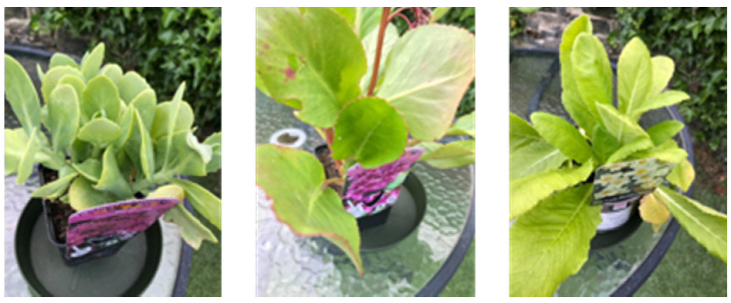
Figure 1. Left to right: Sedum spectabile, Bergenia cordfolia and Primula vulgaris.
Water 13 02262 g001
Figure 2. Leaf stomatal resistance values from the S. spectabile, B. cordfolia and P. vulgaris species between 16 and 18 June 2020.
Water 13 02262 g002
Figure 3. Average leaf temperature (TL) from S. spectabile, B. cordfolia and P. vulgaris species and local air temperature (Ta) over 9 hourly periods between 16 and 18 June 2020.
Water 13 02262 g003
Figure 4. Wind speed and relative humidity measured in each hourly investigative period between 16 and 18 June 2020.
Water 13 02262 g004
Figure 5. Single leaf ET rates found via porometry for S. spectabile, B. cordfolia and P. vulgaris species. Data shown are between 16–18 June in each measurement session.
Water 13 02262 g005
Figure 6. ET rates found via porometry and the mass loss method for the S. spectabile, B. cordfolia and P. vulgaris species. Data shown are between 16–18 June.
Water 13 02262 g006
Figure 7. Scatter plots comparing the ET results from the mass loss and porometry methods.
Water 13 02262 g007
Figure 8. Calculated PET, measurements of ET (via mass loss method, for each plant) and soil water content decrease, SW, (for each plant) between 16–18 June 2020.
Water 13 02262 g008
Table 1. Basic properties of Sedum spectabile, Bergenia cordfolia and Primula vulgaris.
Plant 1, Sedum spectabilePlant 2, Bergenia cordfoliaPlant 3, Primula vulgaris
Small ‘succulent species’ leaf type.
Drought tolerant.
Evergreen, flowering plant.
Dense canopy.
Expected low ET.
Medium sized broad shape leaf.
Requires regular irrigation.
Evergreen, flowering plant.
Dense canopy.
Expected medium ET.
Large, long broad shaped leaf.
Requires regular irrigation.
Evergreen, flowering plant.
Sprawling canopy.
Expected high ET.
Table 2. Leaf area index values of Sedum spectabile, Bergenia cordfolia and Primula vulgaris.
LAIPlant Species
Sedum spectabileBergenia cordifoliaPrimula vulgaris
LAImid7.36.95.9
LAIold0.41.40.6
LAIyng1.50.70.9
Publisher’s Note: MDPI stays neutral with regard to jurisdictional claims in published maps and institutional affiliations.

