A Model for Selecting the Most Cost-Effective Pressure Control Device for More Sustainable Water Supply Networks


Abstract
1. Introduction
2. Methodology
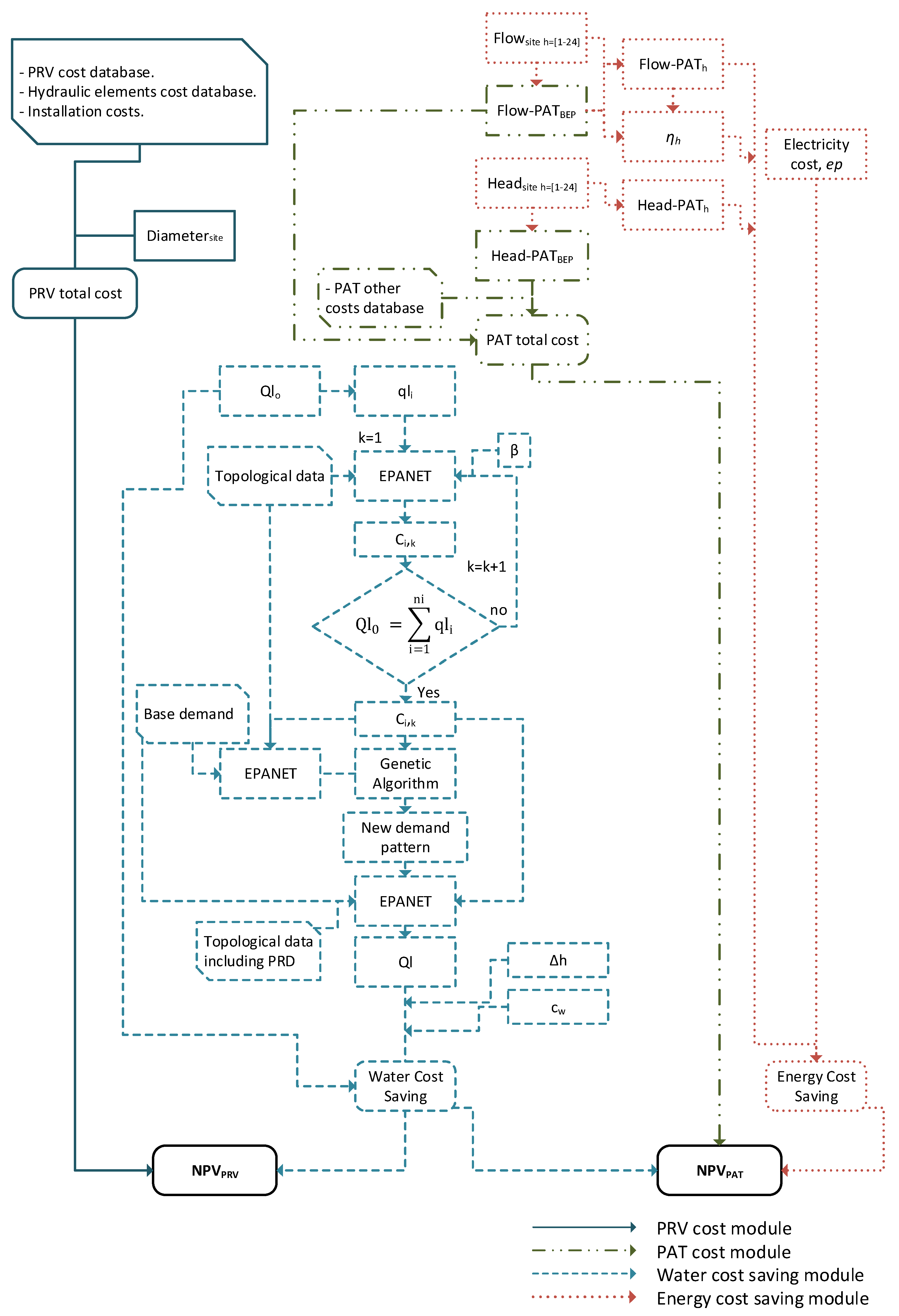
2.1. Problem Approach
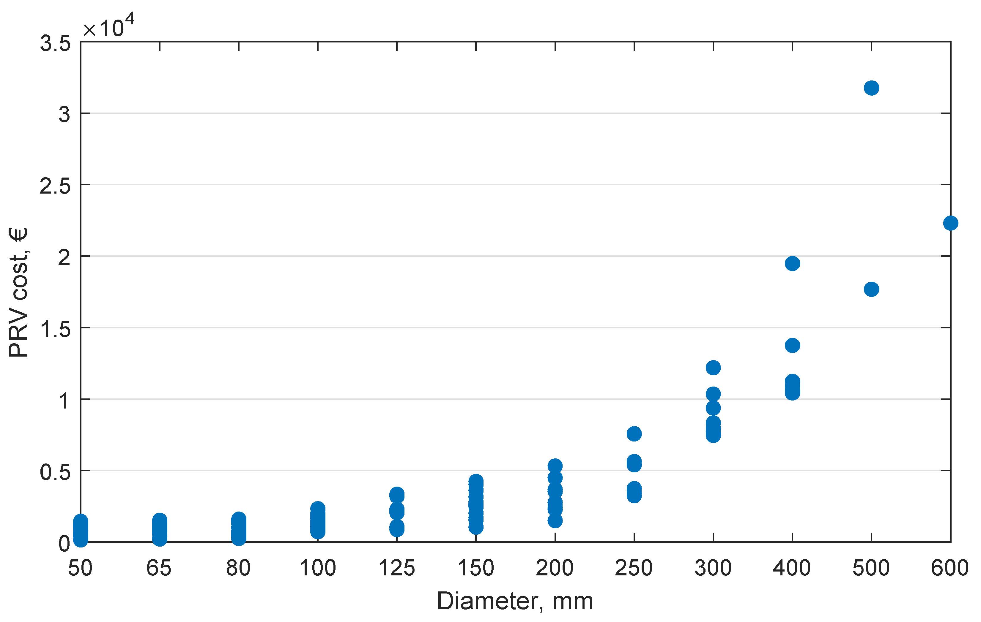
2.2. PRV Total Installation Costs
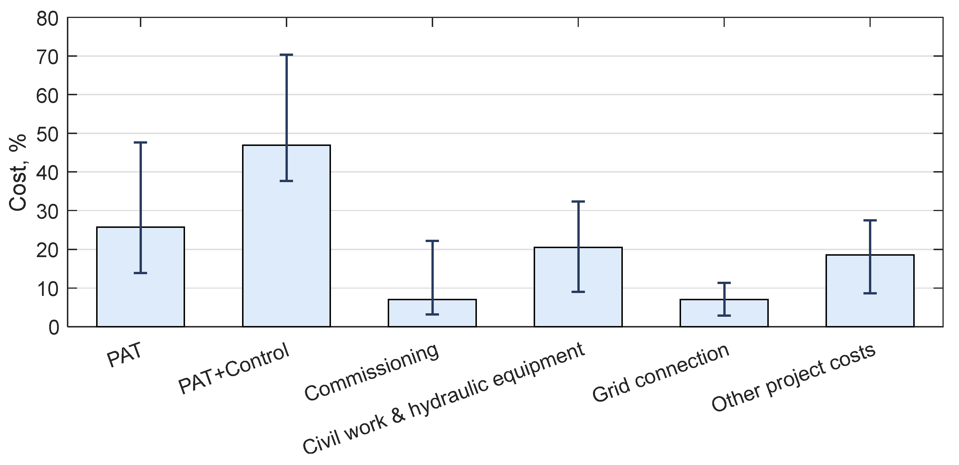
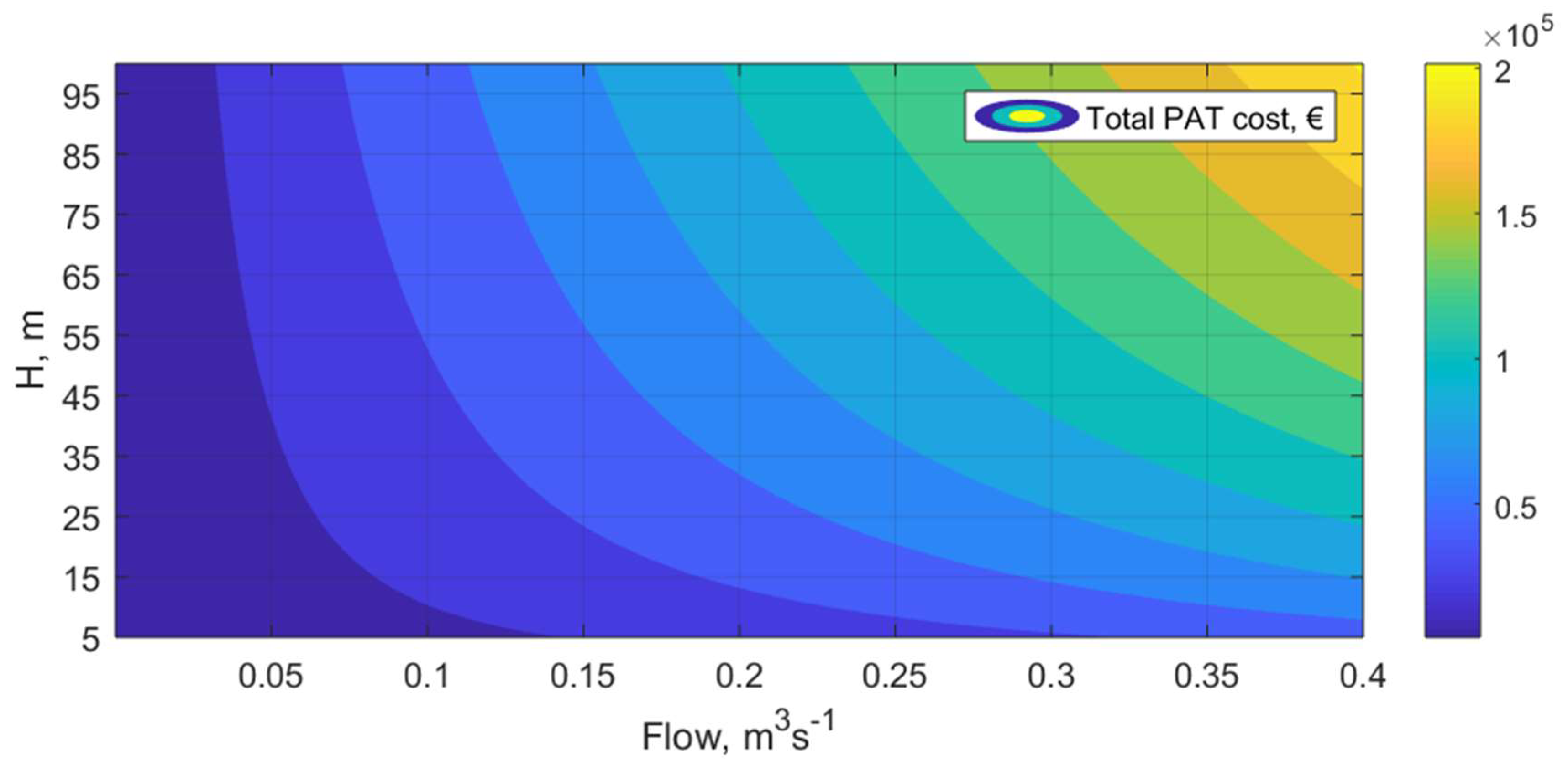
2.3. PAT Total Installation Cost
- -
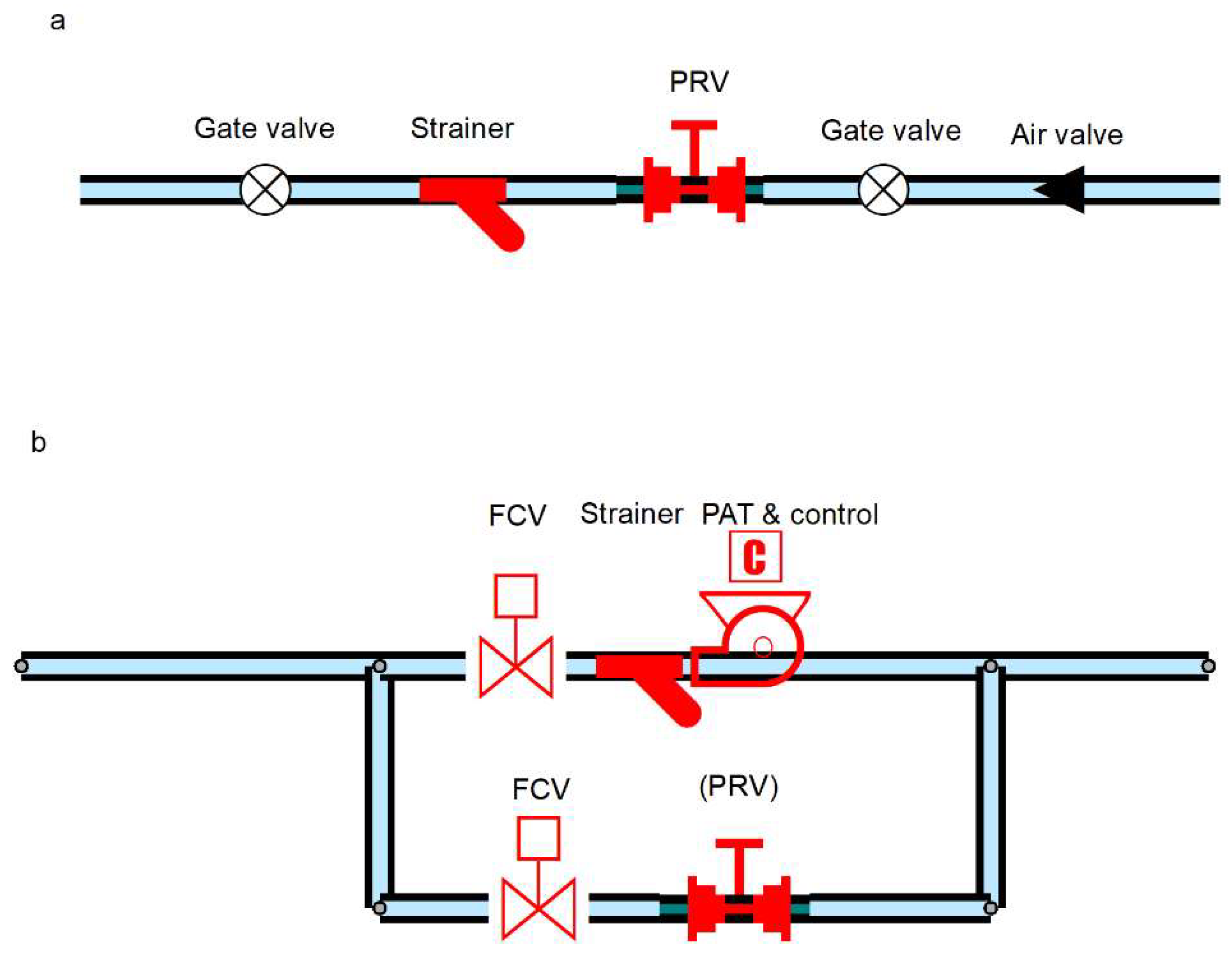
- Civil works and hydraulic equipment, including:
- ○
- a bypass pipe;
- ○
- a set of actuated or manually operated control and sectioning valves;
- ○
- a PRV (in certain installations). The necessity of installing this device depends on whether the PAT will operate far from its BEP at a given site, and the capability of the actuated valves to control the pressure received at downstream nodes. If the pressure is too high to be controlled by the actuated control valves, a PRV installed in the bypass is required.
- ○
- a Y-strainer;
- ○
- a powerhouse hosting the equipment.
- -
- Electric cabinet and control system
- -
- Grid connection fee
- -
- Commissioning
- -
- Other project costs (including consultancy)
- -
- turbogenerator alone;
- -
- turbogenerator and control system;
- -
- commissioning;
- -
- civil works and hydraulic equipment;
- -
- grid connection;
- -
- other project costs.
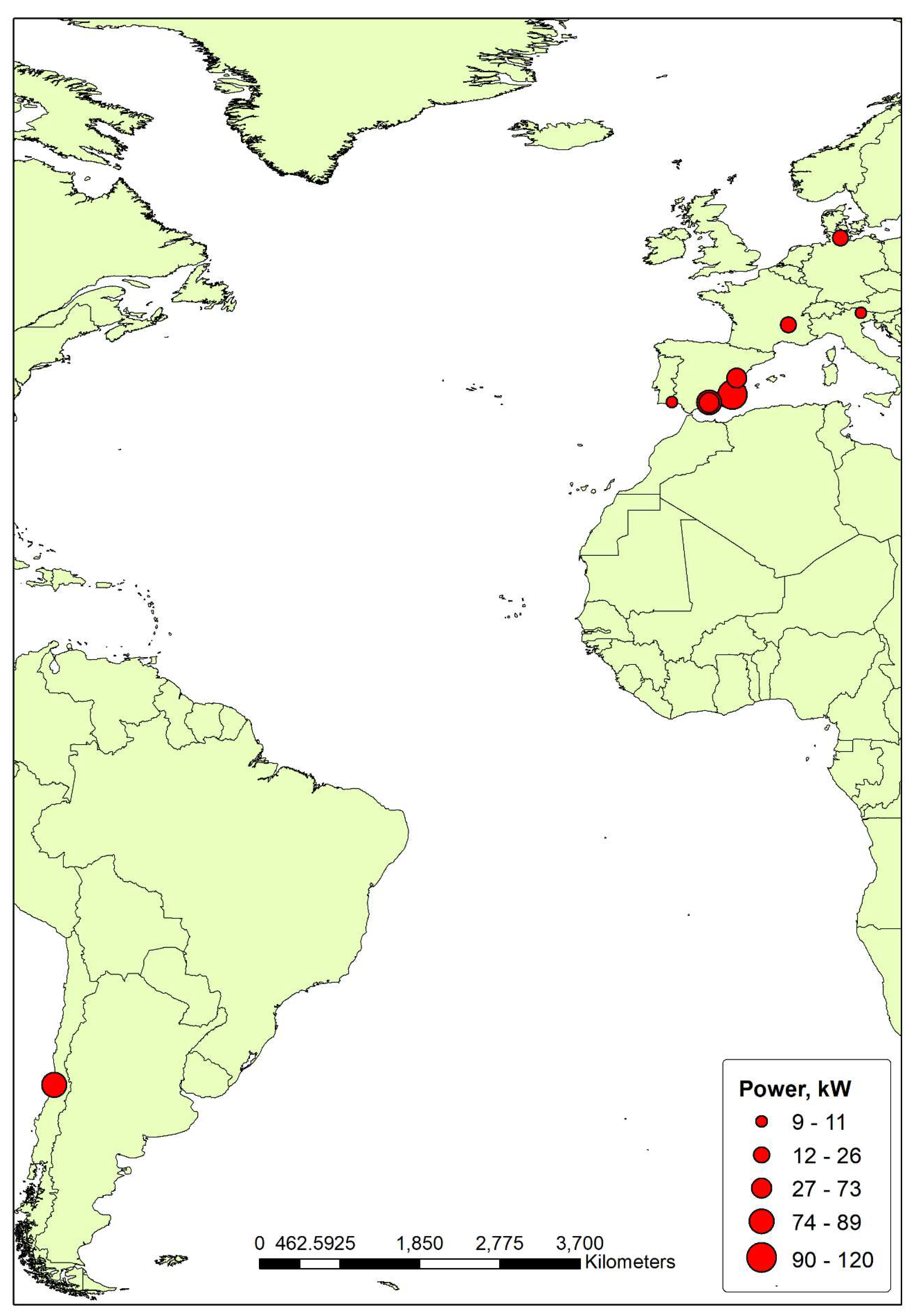
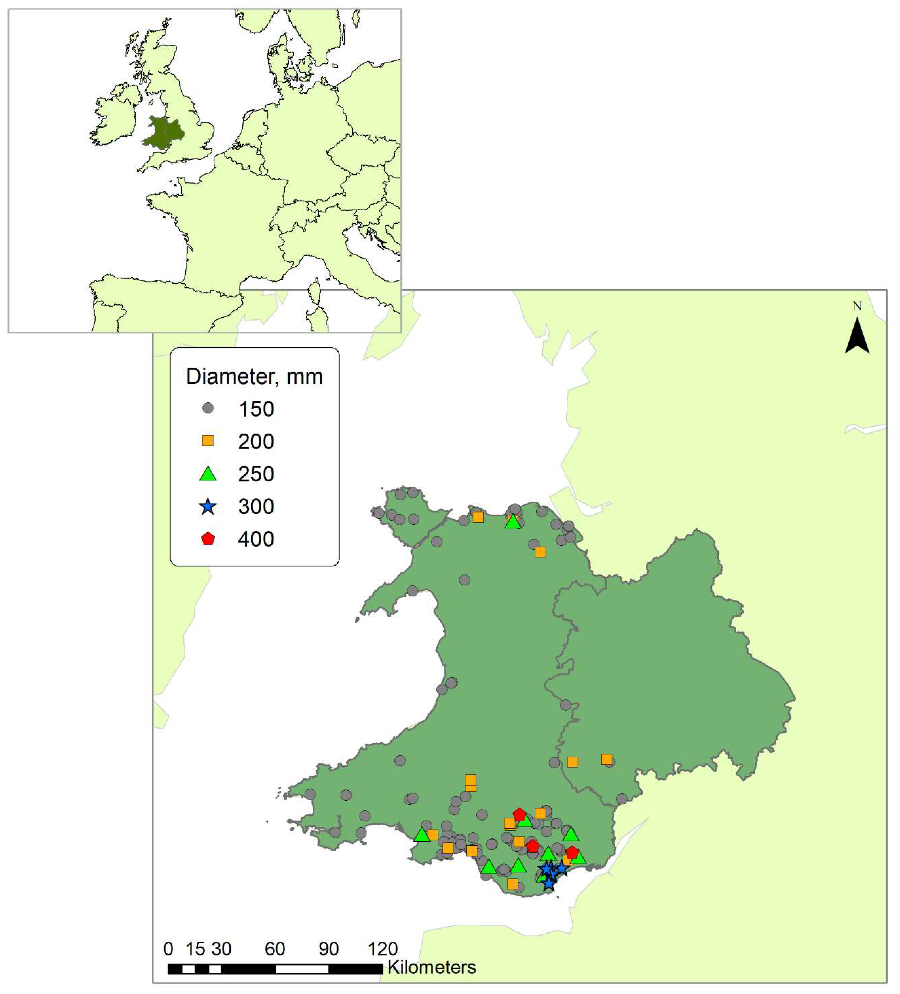
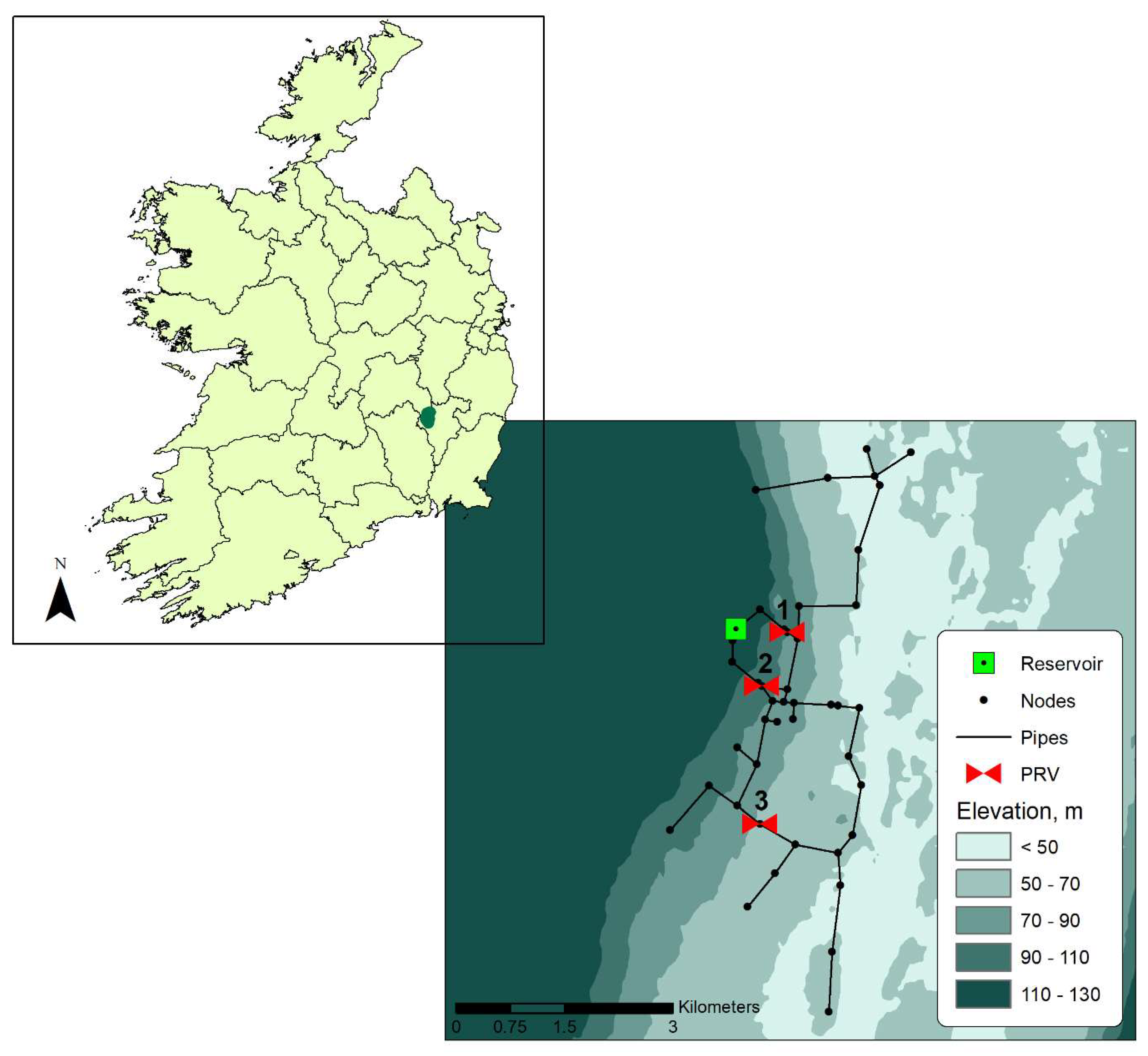
2.4. Case Studies
3. Results
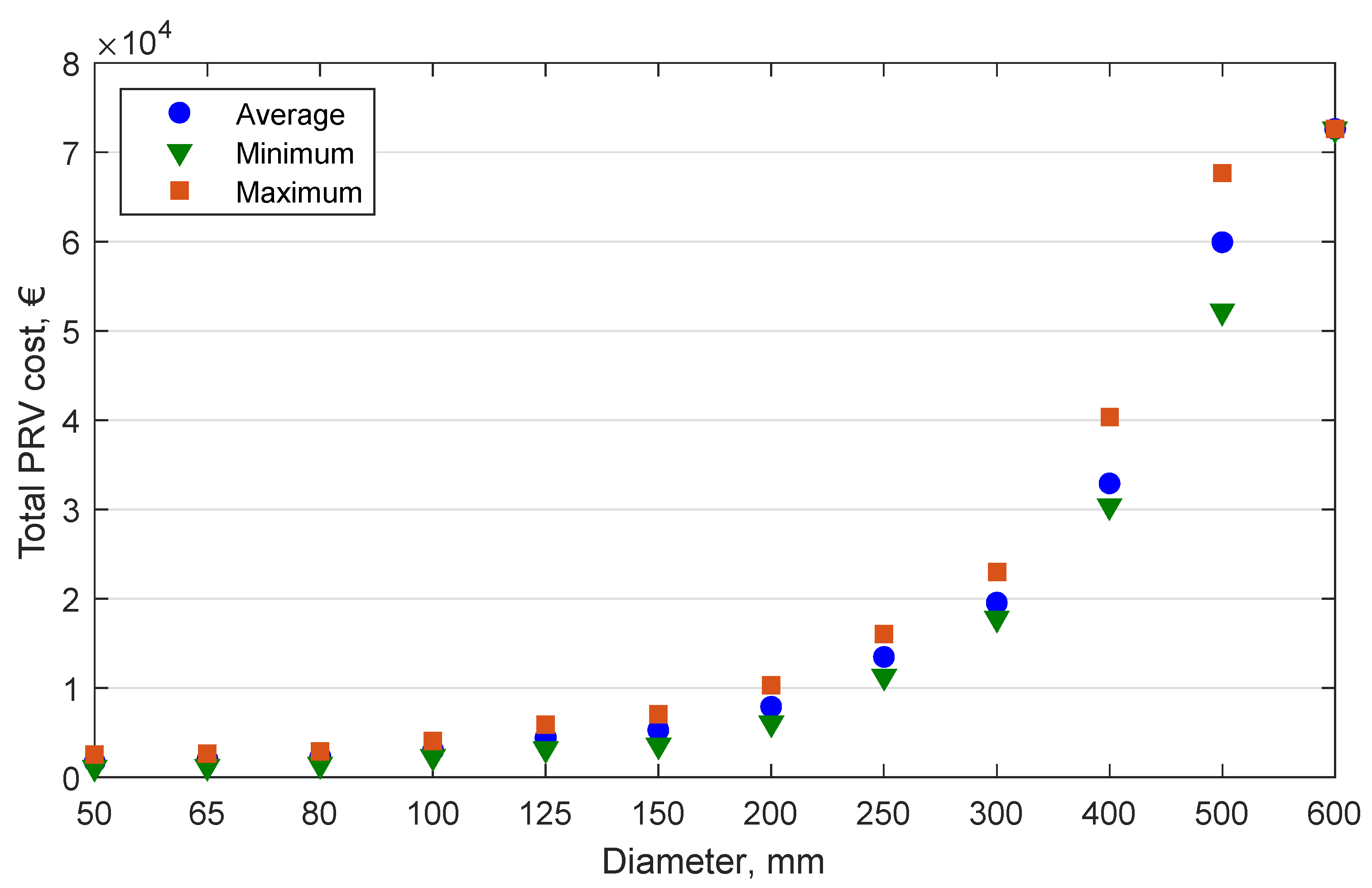
3.1. PRV Cost Model
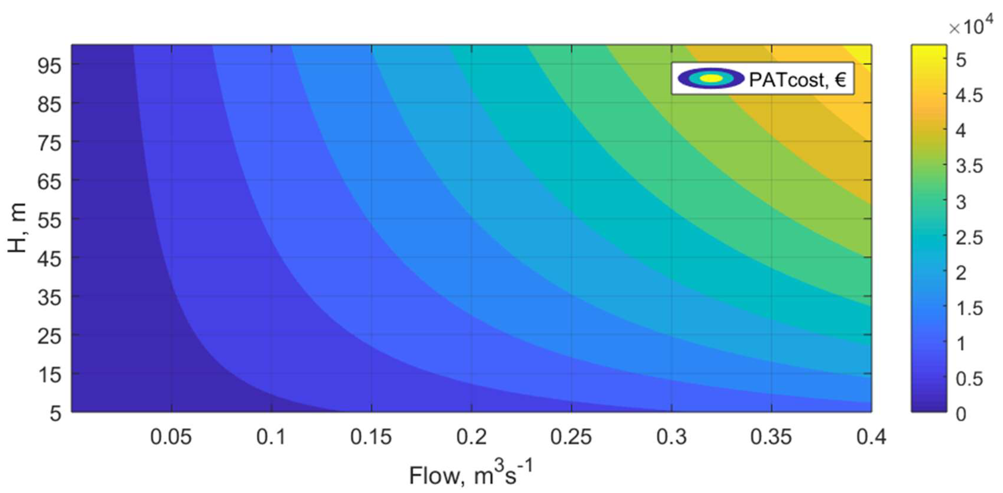
3.2. PAT Cost Model
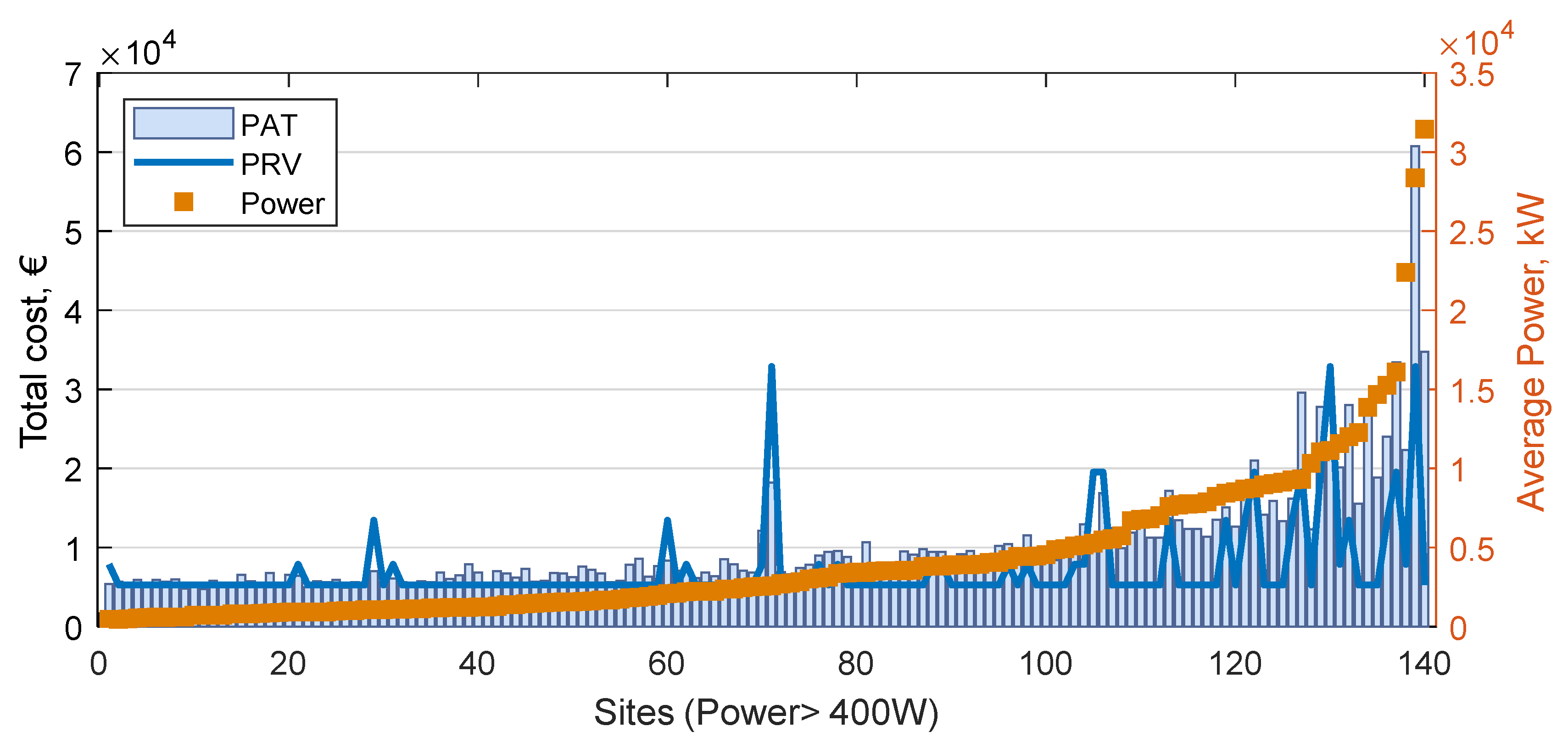
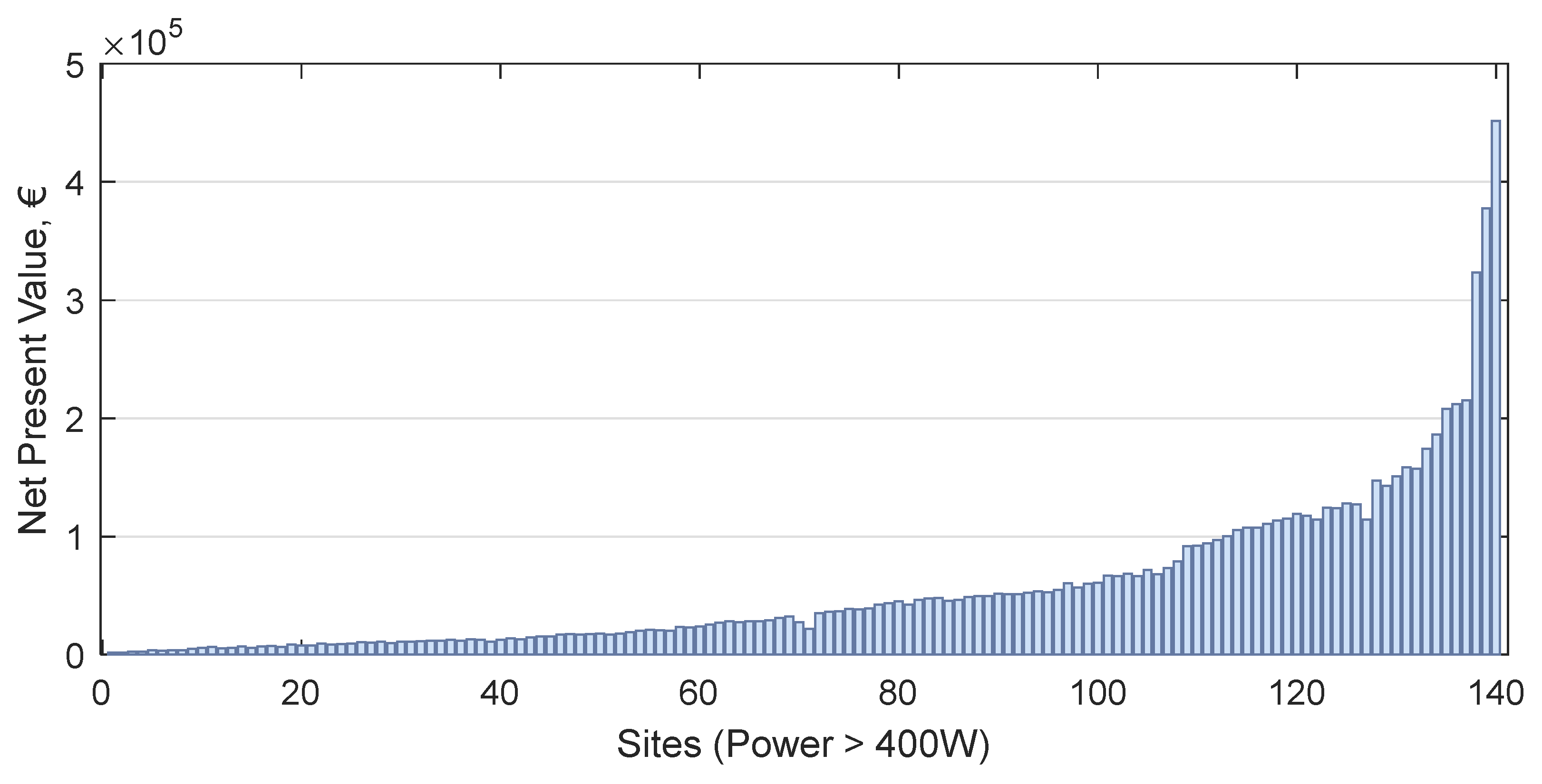
3.3. Determination of the Most Feasible Pressure Reduction Device, PRV or PAT, in the Case Studies
4. Discussion
5. Conclusions
Author Contributions
Funding
Conflicts of Interest
References
- WWAP (United Nations World Water Assessment Programme). The United Nations World Water Development Report 2018: Nature-Based Solutions for Water; WWAP: Paris, France, 2018. [Google Scholar]
- Singh, L.K.; Jha, M.K.; Chowdary, V.M. Multi-criteria analysis and GIS modeling for identifying prospective water harvesting and artificial recharge sites for sustainable water supply. J. Clean. Prod. 2017, 142, 1436–1456. [Google Scholar] [CrossRef]
- McDonald, R.I.; Weber, K.; Padowski, J.; Flörke, M.; Schneider, C.; Green, P.A.; Gleeson, T.; Eckman, S.; Lehner, B.; Balk, D.; et al. Water on an urban planet: Urbanization and the reach of urban water infrastructure. Glob. Environ. Chang. 2014, 27, 96–105. [Google Scholar] [CrossRef]
- European Environment Agency. Use of Freshwater Resources. Available online: https://www.eea.europa.eu/data-and-maps/indicators/use-of-freshwater-resources-2/assessment-2 (accessed on 24 May 2018).
- U.S. Energy Information Administration. International Energy Outlook. 2017. Available online: www.eia.gov/ieo (accessed on 24 May 2018).
- Enerdata. Enerdata World Energy Consumption Statistics. Available online: https://yearbook.enerdata.net/total-energy/world-consumption-statistics.html (accessed on 14 February 2018).
- World-Bank. What is Non-Revenue Water? How Can We Reduce It for Better Water Service? Available online: https://blogs.worldbank.org/water/what-non-revenue-water-how-can-we-reduce-it-better-water-service (accessed on 5 June 2019).
- Loureiro, D.; Amado, C.; Martins, A.; Vitorino, D.; Mamade, A.; Coelho, S.T. Water distribution systems flow monitoring and anomalous event detection: A practical approach. Urban. Water J. 2016, 13, 242–252. [Google Scholar] [CrossRef]
- Mérida García, A.; Fernández García, I.; Camacho Poyato, E.; Montesinos Barrios, P.; Rodríguez Díaz, J.A. Coupling irrigation scheduling with solar energy production in a smart irrigation management system. J. Clean. Prod. 2018, 175, 670–682. [Google Scholar] [CrossRef]
- Kollmann, R.; Neugebauer, G.; Kretschmer, F.; Truger, B.; Kindermann, H.; Stoeglehner, G.; Ertl, T.; Narodoslawsky, M. Renewable energy from wastewater—Practical aspects of integrating a wastewater treatment plant into local energy supply concepts. J. Clean. Prod. 2017, 155, 119–129. [Google Scholar] [CrossRef]
- Gupta, A.; Dpt, C.; National, V.; Bokde, N.; Dpt, C.; National, V.; Marathe, D.; Dpt, C.; National, V.; Kulat, K.; et al. Leakage Reduction in Water Distribution Systems with Efficient Placement and Control of Pressure Reducing Valves Using Soft Computing Techniques. Eng. Technol. Appl. Sci. Res. 2017, 7, 1528–1534. [Google Scholar]
- Parra, S.; Krause, S.; Krönlein, F.; Günthert, F.W.; Klunke, T. Intelligent pressure management by pumps as turbines in water distribution systems: Results of experimentation. Water Sci. Technol. Water Supply 2017, 6, ws2017154. [Google Scholar] [CrossRef]
- Fontana, N.; Giugni, M.; Glielmo, L.; Marini, G.; Zollo, R. Real-Time Control of Pressure for Leakage Reduction in Water Distribution Network: Field Experiments. J. Water Resour. Plan. Manag. 2018, 144, 04017096. [Google Scholar] [CrossRef]
- Gallagher, J.; Styles, D.; McNabola, A.; Williams, A.P. Life cycle environmental balance and greenhouse gas mitigation potential of micro-hydropower energy recovery in the water industry. J. Clean. Prod. 2015, 99, 152–159. [Google Scholar] [CrossRef]
- Lydon, T.; Coughlan, P.; McNabola, A. Pressure management and energy recovery in water distribution networks: Development of design and selection methodologies using three pump-as-turbine case studies. Renew. Energy 2017, 114, 1038–1050. [Google Scholar] [CrossRef]
- McNabola, A.; Coughlan, P.; Corcoran, L.; Power, C.; Prysor Williams, A.; Harris, I.; Gallagher, J.; Styles, D. Energy recovery in the water industry using micro-hydropower: An opportunity to improve sustainability. Water Policy 2014, 16, 168. [Google Scholar] [CrossRef]
- Power, C.; Coughlan, P.; McNabola, A. Microhydropower Energy Recovery at Wastewater-Treatment Plants: Turbine Selection and Optimization. J. Energy Eng. 2017, 143, 04016036. [Google Scholar] [CrossRef]
- Gallagher, J.; Harris, I.M.; Packwood, A.J.; McNabola, A.; Williams, A.P. A strategic assessment of micro-hydropower in the UK and Irish water industry: Identifying technical and economic constraints. Renew. Energy 2015, 81, 808–815. [Google Scholar] [CrossRef]
- Sinagra, M.; Sammartano, V.; Morreale, G.; Tucciarelli, T. A New Device for Pressure Control and Energy Recovery in Water Distribution Networks. Water 2017, 9, 309. [Google Scholar] [CrossRef]
- Samora, I.; Manso, P.; Franca, M.; Schleiss, A.; Ramos, H. Energy Recovery Using Micro-Hydropower Technology in Water Supply Systems: The Case Study of the City of Fribourg. Water 2016, 8, 344. [Google Scholar] [CrossRef]
- Sammartano, V.; Sinagra, M.; Filianoti, P.; Tucciarelli, T. A Banki–Michell turbine for in-line water supply systems. J. Hydraul. Res. 2017, 55, 686–694. [Google Scholar] [CrossRef]
- Sinagra, M.; Aricò, C.; Tucciarelli, T.; Amato, P.; Fiorino, M.; Sinagra, M.; Aricò, C.; Tucciarelli, T.; Amato, P.; Fiorino, M. Coupled Electric and Hydraulic Control of a PRS Turbine in a Real Transport Water Network. Water 2019, 11, 1194. [Google Scholar] [CrossRef]
- Carravetta, A.; del Giudice, G.; Fecarotta, O.; Ramos, H. PAT Design Strategy for Energy Recovery in Water Distribution Networks by Electrical Regulation. Energies 2013, 6, 411–424. [Google Scholar] [CrossRef]
- Carravetta, A.; Derakhshan Houreh, S.; Ramos, H.M. Application of PAT Technology; Springer International Publishing: Berlin/Heidelberg, Germany, 2018; pp. 189–218. [Google Scholar]
- Fecarotta, O.; McNabola, A. Optimal Location of Pump as Turbines (PATs) in Water Distribution Networks to Recover Energy and Reduce Leakage. Water Resour. Manag. 2017, 31, 5043–5059. [Google Scholar] [CrossRef]
- Novara, D.; Carravetta, A.; Derakhshan, S.; McNabola, A.; Ramos, H.M. A Cost model for Pumps as Turbines and a comparison of design strategies for their use as energy recovery devices in Water Supply Systems. In Proceedings of the 10th International Conference on Energy Efficiency in Motor Driven Systems (EEMODS’17), Rome Italy, 6–8 September 2017. [Google Scholar]
- Giugni, M.; Fontana, N.; Ranucci, A. Optimal Location of PRVs and Turbines in Water Distribution Systems. J. Water Resour. Plan. Manag. 2014, 140, 1–6. [Google Scholar] [CrossRef]
- Tricarico, C.; Morley, M.S.; Gargano, R.; Kapelan, Z.; Savić, D.; Santopietro, S.; Granata, F.; de Marinis, G. Optimal energy recovery by means of pumps as turbines (PATs) for improved WDS management. Water Sci. Technol. Water Supply 2018, 184, 1365–1374. [Google Scholar] [CrossRef]
- Pérez-Sánchez, M.; Sánchez-Romero, F.; Ramos, H.; López-Jiménez, P.A. Optimization Strategy for Improving the Energy Efficiency of Irrigation Systems by Micro Hydropower: Practical Application. Water 2017, 9, 799. [Google Scholar] [CrossRef]
- García Morillo, J.; McNabola, A.; Camacho, E.; Montesinos, P.; Rodríguez Díaz, J.A. Hydro-power energy recovery in pressurized irrigation networks: A case study of an Irrigation District in the South of Spain. Agric. Water Manag. 2018, 204, 17–27. [Google Scholar] [CrossRef]
- Fecarotta, O.; Aricò, C.; Carravetta, A.; Martino, R.; Ramos, H.M. Hydropower Potential in Water Distribution Networks: Pressure Control by PATs. Water Resour. Manag. 2015, 29, 699–714. [Google Scholar] [CrossRef]
- Patelis, M.; Kanakoudis, V.; Gonelas, K. Pressure Management and Energy Recovery Capabilities Using PATs. Procedia Eng. 2016, 162, 503–510. [Google Scholar] [CrossRef]
- The Public Spending Code. Ireland Department of Public Expenditure and Reform E-Technical References. Available online: http://publicspendingcode.per.gov.ie/technical-references/ (accessed on 14 May 2018).
- Araujo, L.S.; Ramos, H.; Coelho, S.T. Pressure Control for Leakage Minimisation in Water Distribution Systems Management. Water Resour. Manag. 2006, 20, 133–149. [Google Scholar] [CrossRef]
- Rossman, L.A. EPANET 2 Users Manual EPA/600/R-00/57; U.S. Environmental Protection Agency: Cincinnati, OH, USA, 2000.
- Araujo, L.S.; Ramos, H.; Coelho, S.T. Estimation of distributed pressure-dependent leakage and consumer demand inwater supply networks. In Advance in Water Supply Management; CRC Press: London, UK, 2003. [Google Scholar]
- Fernández García, I.; Ferras, D.; McNabola, A. Potential of energy recovery and water saving using microhydropower in rural water distribution networks. J. Water Resour. Plan. Manag. 2019, 145, 1–11. [Google Scholar] [CrossRef]
- The MathWorks Inc. MATLAB Version R2016b; The MathWorks Inc.: Natick, MA, USA, 2016. [Google Scholar]
- SEAI. Electricity & Gas Prices in Ireland. 1st Semester (January–June) 2017. Available online: https://www.seai.ie/resources/publications/Electricity_Gas_Prices_January_June_2017 (accessed on 10 May 2018).
- Carravetta, A.; Fecarotta, O.; Ramos, H.M. A new low-cost installation scheme of PATs for pico-hydropower to recover energy in residential areas. Renew. Energy 2018, 125, 1003–1014. [Google Scholar] [CrossRef]
- Fecarotta, O.; Ramos, H.M.; Derakhshan, S.; Del Giudice, G.; Carravetta, A. Fine Tuning a PAT Hydropower Plant in a Water Supply Network to Improve System Effectiveness. J. Water Resour. Plan. Manag. 2018, 144, 04018038. [Google Scholar] [CrossRef]
- Novara, D.; McNabola, A. A model for the extrapolation of the characteristic curves of Pumps as Turbines from a datum Best Efficiency Point. Energy Convers. Manag. 2018, 174, 1–7. [Google Scholar] [CrossRef]
- Grancho Ferreira, A.R. Energy Recovery in Water Distribution Networks towards Smart Water Grids. Master’s Thesis, University of Lisbon, Lisbon, Portugal, 2017. [Google Scholar]
- BERMAD PRV cost. Personal Communication, 2018.
- CLA-VAL PRV cost. Personal Communication, 2018.
- WATTs PRV cost. Personal Communication, 2018.
- Flomatic PRV cost. Personal Communication, 2018.
- AVK PRV cost. Personal Communication, 2018.
- CSA PRV cost. Personal Communication, 2018.
- Valves-Online PRV cost. Personal Communication, 2018.
- Talis PRV cost. Personal Communication, 2018.
- TRAGSA Tarifas 2015 Para Encomiendas Sujetas a Impuestos. 2015. Available online: https://www.tragsa.es/es/grupo-tragsa/regimen-juridico/Documents/ACTUALIZACI%C3%93N%20TARIFAS%20AGOSTO/Tarifas%202015%20para%20encomiendas%20sujetas%20a%20impuestos.pdf (accessed on 20 June 2019).
- Novara, D.; Carravetta, A.; McNabola, A.; Ramos, H.M. Cost model for Pumps As Turbines in run-off-river and in-pipe micro-hydropower applications. J. Water Resour. Plan. Manag. 2019, 145, 04019012. [Google Scholar] [CrossRef]
- Ogayar, B.; Vidal, P.G. Cost determination of the electro-mechanical equipment of a small hydro-power plant. Renew. Energy 2009, 34, 6–13. [Google Scholar] [CrossRef]
- Kramer, M.; Terheiden, K.; Wieprecht, S. Pumps as turbines for efficient energy recovery in water supply networks. Renew. Energy 2018, 122, 17–25. [Google Scholar] [CrossRef]
- Livramento, J.M. Central micro-hídrica incorporada em adutora. Master’s Thesis, Faculdade de Ciências e Tecnologia, Universidade do Algarve, Faro, Portugal, 2013. [Google Scholar]
- Lledó, J. Tecnoturbines. Powering Water 2016. Available online: https://www.mapa.gob.es/images/es/tt-center_tcm30-131554.pdf (accessed on 20 June 2019).
- Alkasseh, J.M.A.; Adlan, M.N.; Abustan, I.; Aziz, H.A.; Hanif, A.B.M. Applying Minimum Night Flow to Estimate Water Loss Using Statistical Modeling: A Case Study in Kinta Valley, Malaysia. Water Resour. Manag. 2013, 27, 1439–1455. [Google Scholar] [CrossRef]
- Ramos, H.; Borga, A. Pumps as turbines: An unconventional solution to energy production. Urban. Water 1999, 1, 261–263. [Google Scholar] [CrossRef]
- Pérez-Sánchez, M.; Sánchez-Romero, F.J.; López-Jiménez, P.A.; Ramos, H.M. PATs selection towards sustainability in irrigation networks: Simulated annealing as a water management tool. Renew. Energy 2018, 116, 234–249. [Google Scholar] [CrossRef]


| Diameter, mm | ||||||||||||
|---|---|---|---|---|---|---|---|---|---|---|---|---|
| 50 | 65 | 80 | 100 | 125 | 150 | 200 | 250 | 300 | 400 | 500 | 600 | |
| Gate valve (2) | 146 | 190 | 218 | 274 | 374 | 514 | 800 | 1216 | 1676 | 2899 | 4462 | 6370 |
| Strainer | 148 | 159 | 208 | 227 | 410 | 391 | 717 | 1377 | 2104 | 5331 | 11,669 | 18,063 |
| Air valve | 543 | 543 | 615 | 854 | 1215 | 1290 | 2520 | 4430 | 4947 | 8953 | 13,624 | 19,286 |
| TOTAL | 837 | 892 | 1041 | 1355 | 1999 | 2195 | 4037 | 7023 | 8727 | 17,183 | 29,756 | 43,719 |
| Power, kW | Total PRV Cost, € | Total PAT Cost, € | PAT NPV, € | PAT Payback Period, years | |||||||
|---|---|---|---|---|---|---|---|---|---|---|---|
| 26% 1 | 48% 2 | 14% 3 | 26% 1 | 48% 2 | 14% 3 | 26% 1 | 48% 2 | 14% 3 | |||
| Ave. | 4338 | 7236 | 10,397 | 5567 | 20,831 | 57,960 | 61,489 | 59,163 | 4 | 3 | 6 |
| Max. | 31,455 | 32,909 | 60,770 | 32,862 | 112,534 | 451,467 | 467,421 | 421,875 | 10 | 7 | 10 |
| Min. | 460 | 5284 | 4761 | 2575 | 9097 | 2695 | 4197 | 5079 | 2 | 2 | 3 |
| PRV | PAT | |||||
|---|---|---|---|---|---|---|
| Site Number | 1 | 2 | 3 | 1 | 2 | 3 |
| Diameter, mm | 150 | 100 | 100 | 150 | 100 | 100 |
| Power BEP, W | 1223 | 1533 | 457 | |||
| Energy, kWh year−1 | 7346 | 9203 | 2744 | |||
| Ave cost, € | 5284 | 3009 | 3009 | 5919 | 6268 | 5323 |
| Min cost, € | 3574 | 2303 | 2303 | 3201 | 3390 | 2879 |
| Max cost, € | 7074 | 4067 | 4067 | 10,984 | 11,633 | 9879 |
| Water saving, m3 year−1 | 15,559 | 15,559 | 15,559 | 15,559 | 15,559 | 15,559 |
| Water cost saving, € year−1 | 4668 | 4668 | 4668 | 4668 | 4668 | 4668 |
| Energy cost saving, € year−1 | 1249 | 1565 | 466 | |||
| Payback period, year | 3.0 | 2.0 | 2.0 | 3.0 | 3.0 | 3.0 |
| NPV, € | 43,164 | 45,440 | 45,440 | 55,493 | 58,420 | 47,967 |
| NPV/Water saving, € m−3 | 0.18 | 0.19 | 0.19 | 0.24 | 0.25 | 0.21 |
© 2019 by the authors. Licensee MDPI, Basel, Switzerland. This article is an open access article distributed under the terms and conditions of the Creative Commons Attribution (CC BY) license (http://creativecommons.org/licenses/by/4.0/).
Share and Cite
García, I.F.; Novara, D.; Mc Nabola, A. A Model for Selecting the Most Cost-Effective Pressure Control Device for More Sustainable Water Supply Networks. Water 2019, 11, 1297. https://doi.org/10.3390/w11061297
García IF, Novara D, Mc Nabola A. A Model for Selecting the Most Cost-Effective Pressure Control Device for More Sustainable Water Supply Networks. Water. 2019; 11(6):1297. https://doi.org/10.3390/w11061297
Chicago/Turabian StyleGarcía, Irene Fernández, Daniele Novara, and Aonghus Mc Nabola. 2019. "A Model for Selecting the Most Cost-Effective Pressure Control Device for More Sustainable Water Supply Networks" Water 11, no. 6: 1297. https://doi.org/10.3390/w11061297
APA StyleGarcía, I. F., Novara, D., & Mc Nabola, A. (2019). A Model for Selecting the Most Cost-Effective Pressure Control Device for More Sustainable Water Supply Networks. Water, 11(6), 1297. https://doi.org/10.3390/w11061297