Abstract
This study presents a simple mapping key suitable for quick and systematic assessments of the types of agricultural and civil engineering structures present in a certain agricultural catchment as well as the impact they may have on the spatial distribution of critical source areas. An application of this mapping key to three small sub-catchments of a case study catchment with an area of several hundred square kilometres (one-stage cluster sampling) in Austria clearly reveals that road embankments with subsurface drainage can exert a major influence on emissions and transport pathways of sediment-bound pollutants like particulate phosphorus (PP). Due to this, the semi-empirical, spatially distributed PhosFate model is extended to separately model PP emissions into surface waters via storm drains along road embankments. Furthermore, the overall share of road embankments with subsurface drainage on all road embankments in the case study catchment is inferred with the help of a Bayesian hierarchical model. The combination of the results of these two models shows that the share of storm drains at road embankments on total PP emissions ranges from about one fifth to one third in the investigated area.
1. Introduction
Many efforts to control diffuse pollution of surface waters in agricultural catchments are based on the concept of critical source areas. This concept commonly refers to relevant source areas connected to surface waters in a way that allows significant amounts of pollutants to enter surface waters (e.g., [1,2,3]). While the concept of critical source areas is basically applicable to many different pollutants, it is particularly relevant in the case of particulate phosphorus (PP) and other sediment-bound emissions.
PP emissions in agricultural catchments are in fact often dominated by soil erosion processes and PP transport into surface waters by overland flow. In this context, a common approach to identify critical source areas is the use of spatially distributed models. De Vente et al. [4] compared different models developed to predict soil erosion rates, sediment yield and in case of spatially distributed models also sediment sources and sinks. They conclude that while empirical/conceptual, spatially distributed models show good model performances in comparison to data requirements, the application of this type of models is only appropriate in cases where the considered erosion (e.g., sheet, rill and ephemeral gully erosion) and sediment transport processes (e.g., overland flow, soil creep and debris flow) effectively dominate the catchment of interest.
This implies that in order to successfully apply such a model to a certain catchment, a priori knowledge on its dominant erosion and sediment transport processes as well as pathways is required. Jetten et al. [5] even advocate including observed patterns in modelling studies, since this can greatly improve model results. Such knowledge, however, is only scarcely available.
A number of studies report that agricultural and civil engineering structures (e.g., roads, ditches and culverts) may exert a decisive influence on erosion and sediment transport within catchments. Roads are found to “accelerate water flows and sediment transport” [6] and are responsible for altering flow routing patterns as well as slope lengths [7,8]. Particularly in combination with roadside ditches and culverts, they can directly connect sections of catchment areas to stream networks, which otherwise would only be indirectly connected or not connected at all [9,10,11,12,13,14].
Moussa et al. [15] furthermore point out that inter-field ditch networks increase the portions of catchment areas directly contributing to the discharge of surface waters. In short, linear agricultural and civil engineering structures hold a large potential to boost direct pollutant emissions into surface waters even from remote and at first glance disconnected fields.
This a priori knowledge is very valuable when it comes to applying a model to a certain catchment. In case of catchments where roads play a major role, they are capable of extending the natural stream network considerably. Or to say it with the words of Hösl et al. [12]: “Ditches may occur near almost every road or track to drain road systems.”
Despite all these observations, linear structures are rarely considered in models and modelling studies [16]. A notable exception is the WaTEM/SEDEM model [8,17,18], which optionally takes a roads data layer as additional input. Instead of integrating linear structures into models, there is, however, also the alternative of digital elevation model (DEM) pre-processing. The RIDEM model [19,20] takes this approach. It utilises cross-sectional templates of different configurations of roads and roadside ditches to enforce their effect on flow directions. Although DEM pre-processing has the advantage of not necessarily being dependent on a certain model, it does not seem to be widely applied in the context of linear structures.
While the role of roads and ditches in altering overland flow patterns is generally rather well-known, still vague is the role of another common agricultural and civil engineering structure: storm drains [21]. This point-shaped structure is similarly capable of directly connecting remote fields to surface waters. The main difference to ditches lies in its subsurface transport pathway via sewers. In direct comparison with ditches, this means there is less retention, given that roadside ditches are often at least partly vegetated with grass and occasionally cleaned.
Several applications of the semi-empirical, spatially distributed PhosFate model [22,23] in the Austrian federal state of Upper Austria [24,25] suggest that storm drains may have a significant influence on sediment emissions into surface waters. Verstraeten et al. [26] state that the effect of riparian vegetated buffer strips on catchment scale may be rather low, since a considerable amount of sediment bypasses them through sewers, among others. Another study found that artificial zones like farm courtyards are responsible for about half of the fields connected to the stream network [27]. While they do not decidedly mention storm drains or sewers, it can be reasoned, that they are a major cause of this. In addition, Djodjic and Villa [28] express that surface water inlets are common in Sweden and due attention should be paid to them.
As a result of a field mapping campaign in a catchment in north-western Switzerland, Bug [29] reports that storm drains occur mainly at asphalt roads leading across a hillside and in areas with flow convergence. However, for another catchment in the German federal state of Lower Saxony, he depicts a dense network of ditches but no storm drains at all. This indicates that there exist different traditions in implementing agricultural and civil engineering measures.
Since detailed datasets on the existence of ditches and storm drains are rarely available but a prerequisite for modelling studies aiming at the identification of critical source areas, there is a need to map them. Although several studies have carried out related field mapping campaigns in the past (e.g., [10,12,29]), no ready to use mapping key exists for this task. This study therefore intends to develop, present and discuss a simple mapping key suitable for practitioners interested in a quick and systematic assessment of the types of agricultural and civil engineering structures present in a certain catchment as well as the impact they may have on the spatial distribution of critical source areas.
A further objective is to estimate the share of PP emissions entering surface waters via storm drains and sewers at road embankments. The relevance of these structures is assessed for a case study catchment with an area of several hundred square kilometres. This is seen as essential information for policy makers facing the task to meet water quality targets in catchments of similar size.
2. Material and Methods
2.1. Case Study Catchment
This study was performed on the catchment of the river Pram in the Austrian federal state of Upper Austria, which is located in the northern part of the country. Its area is approximately 380 km2 in size and it belongs to the geologic formation Molasse basin with small parts in the north and northeast belonging to the crystalline Bohemian Massif. The prevalent soil texture is silt loam (nearly 50% of the soil surface) followed by other types of loam. Only 5% of the soil surface are dominated by clay. Soil textures dominated by sand are not present in the catchment area.
Annual precipitation ranges from roughly 900 in the north with an elevation of about 300 a. s. l. to around 1200 in the south with an elevation of about 800 a. s. l. Agricultural land (approx. 45% arable land and 25% grassland) is prevailing in the predominantly hilly terrain. Forests account for about 20% and built-up areas for almost 10% of the catchment area. The most important crops are winter grains and maize covering approximately 40 and 30% of the arable land respectively. Additional catchment properties are listed in Table 1. Diffuse PP emissions are totally dominated by erosion from, especially, agricultural land. Other types of sources are negligible [30]. Altogether, anthropogenic influence can be considered as high in this catchment.

Table 1.
Additional properties of the case study catchment.
2.2. Mapping Key
The mapping key was developed based on the hydrological connectivity definitions related to landscape features and hillslope scale as collected by Ali and Roy ([32], Table 1). Among these definitions, the one from Croke et al. [10] distinguishes “two types of connectivity: direct connectivity via new channels or gullies, and diffuse connectivity as surface runoff reaches the stream network via overland flow pathways.”
For this mapping key, the direct connectivity type was extended to include not only channels and gullies but also ditches, culverts, storm drains and sewers. Direct connectivity was furthermore split into known and unknown direct connectivity in order to differentiate between areas connected to an existing (e.g., governmental mapped) stream network dataset and areas connected to the actual stream network via features unknown to such a dataset (cf. [33]). The term diffuse connectivity was kept as it is.
A major issue with all connectivity mapping methods is that they merely record “snapshots” [34]. Within the concept of hydrological connectivity one can distinguish static/structural and dynamic/ functional elements of connectivity [35,36]. A simplified view on these elements comprehends space as structure and space-time as function [37]. Omitting the functional element leads to a purely structural approach, which is solely capable of pointing out potential connectivity [34].
De Vente et al. [4] note that empirical/conceptual, spatially distributed models are frequently built on the RUSLE [38]. Since this erosion model as well as its precursor USLE [39,40] estimate long term yearly erosion rates under average climatic conditions only, which can likewise be considered a potential (erosion potential), they match comparatively well with purely structural connectivity approaches.
Ultimately, the development of this mapping key aimed at aiding practitioners in preparing modelling studies with empirical/conceptual, spatially distributed models for water quality management at catchment scale. It therefore was based on a purely structural approach focusing on discrete mapping units like fields or (parts of) zero-order catchments. With the term zero-order catchments we refer to the catchment areas of all zones in a landscape exhibiting an overland-channel transition (Figure 1).
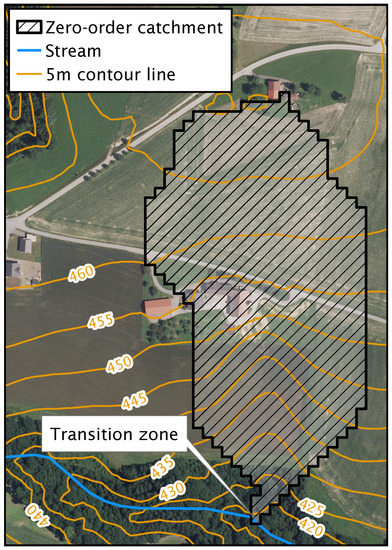
Figure 1.
Example of a zero-order catchment (catchment area belonging to a single overland-channel transition zone) based on a DEM with resolution and the D8 single flow direction algorithm [41].
For each mapping unit, this mapping key fundamentally records if it is (i) connected or (ii) not connected in a natural way and/or if an (additional) artificial connection is (i) present, (ii) not present or (iii) present in a downstream mapping unit. It is thus required to map from downstream to upstream. Both of these types of connectivity are further supported by explanatory details, which include the cause of a mapping unit being connected or not in a natural way and, in case one is present, the type of the artificial connection.
Additionally, this mapping key allows for mapping artificial point-shaped and linear structures as well as natural features like channels missing in existing datasets. This can help with retracing flow pathways in case of questions once the mapping has been completed. The full ready to use and basically adaptable mapping key tables can be found in Appendix A.
Since connectivity is linked, among others, to discharge frequency, especially the categorisation of mapping units regarding connected in a natural way or not is somewhat arbitrary and in danger of subjectivity of the person(s) carrying out a mapping campaign. This issue can be addressed by defining a threshold obstacle height. Mosimann et al. [33] acknowledge obstacles higher than 50 as effective barriers for surface runoff, preventing connectivity, and so do we.
In order to efficiently apply this mapping key, a mobile geographic information system (GIS) supporting a global navigation satellite system (GNSS) with at least two datasets is required: (i) an existing stream network and (ii) borders of the desired mapping units as well as the ability to alter them. Additional digital orthophotos help furthermore with orientation and locating certain landscape features.
2.3. Application of the Mapping Key
For the application of the mapping key, agricultural fields were chosen as mapping units. The statistical population of the case study catchment is therefore the total amount of its fields. Survey sampling was carried out with the help of one-stage cluster sampling. Cluster sampling is particularly useful when the statistical population under consideration can be grouped geographically. In the present case, it was grouped into small sub-catchments, which allowed for minimising travel times.
Generally speaking, one-stage cluster sampling refers to the random selection of a subset of all clusters and the systematic assessment of all elements within the selected clusters. On the contrary, two-stage cluster sampling refers to not only the random selection of a subset of all clusters but also to the random selection of a subset of the elements to be assessed within the selected clusters. In this context, three small sub-catchments/clusters (Figure 2) were randomly selected from the total of 154 small sub-catchments/clusters of the case study catchment. The one-stage cluster sampling was then carried out by systematically mapping all of their fields.
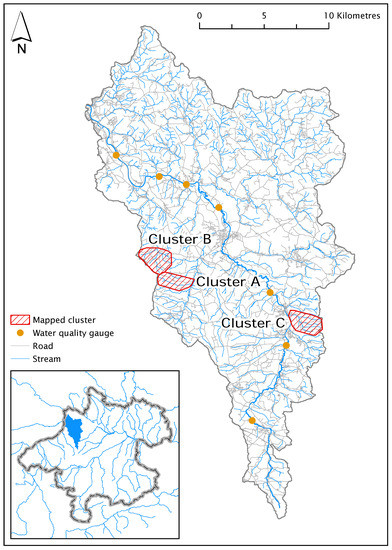
Figure 2.
The case study catchment with the three randomly selected and systematically mapped clusters as well as the seven water quality gauges along the river Pram used for calibrating PhosFate.
For this task, a tablet computer running Microsoft Windows 10 with Esri ArcPad version 10.2.1 employing an external Global Positioning System (GPS) receiver was used. The field borders could be taken from a (geo-)database related to the Integrated Administration and Control System (IACS) of the Common Agricultural Policy (CAP) of the European Union (EU) [42]. A high-quality governmental mapped stream network was available from the Federal Office of Metrology and Surveying [43] and digital orthophotos were contributed by the State Government of Upper Austria. Moreover, for referencing, a picture geodatabase was created containing overview pictures and pictures showing the relevant details of each field.
About 650 of agricultural land corresponding to 323 fields were mapped in total (Table 2). These are approximately 2.5% of the overall agricultural land within the case study catchment. Each mapped cluster has its own characteristics: cluster A is elongated with tendentiously steep slopes and roads mainly on the ridges, cluster B has a tree-like stream network, tendentiously gentle slopes and roads mainly on the ridges as well and cluster C has roads primarily leading across hillsides and partially cased streams. The fairly smaller average field size of cluster C may be due to its roads leading across hillsides, which split more fields apart. While cluster A’s diffuse PP emissions reaching surface waters are with roughly kg ha−1 rather high due to its steep slopes, those of cluster B and C are lower and amount to roughly 1.4 and kg ha−1 respectively.
Table 2.
Mapped agricultural land and number of fields per catchment and agricultural land use type.
2.4. Modelling the Impact of Storm Drains at Road Embankments on PP Transport
2.4.1. The PhosFate Model
PhosFate is a semi-empirical, spatially distributed phosphorus emission and transport model created for the identification of critical source areas in a management context at catchment scale [22,23]. It is based on raster GIS data and utilises the (R)USLE [38,39,40] incorporating a single flow algorithm version of the slope length factor of Desmet and Govers [44]. PP emissions are then calculated from the erosion and PP content of each raster cell considering a local enrichment ratio [24].
The PP transport part of PhosFate consists of the computation of the PP retention via an exponential function of the cell residence time and a mass balance equation considering the inflowing PP load, the local PP emission and the local as well as the transfer PP retention. Computing the cell residence time requires the calculation of the hydraulic radius among others. This variable in turn involves model parameters related to discharge frequency [24]. So again, a potential (transport potential) is calculated. PP transport as calculated by PhosFate thus reflects maximum potential PP transport for a chosen discharge frequency.
2.4.2. Storm Drains Model Extension
The current version of PhosFate does not consider any linear structures potentially influencing PP transport. As a result of the field mapping campaign (see Section 3.1), it was deemed necessary to take storm drains at varying distances along road embankments often in combination with roadside ditches (Figure 3) into account. An algorithm incorporating known locations of storm water infrastructure is the (W)ASI algorithm [45,46]. At catchment scale, however, particularly the locations of rural storm drains are hardly known.
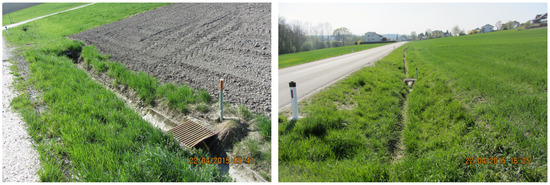
Figure 3.
Roadside ditch with multiple storm drains at varying distances. The left picture was taken upstream of the right.
It was therefore decided to regard every raster cell bordering and flowing in the direction of a road as a storm drain with its outlet at the nearest stream cell (cf., [9]). Since the flow lengths in roadside ditches between the actual locations of surface runoff leaving a field and entering a storm drain remain unknown choosing such an approach, the retention potential in roadside ditches is likewise unknown. Retention in roadside ditches was thus considered globally by means of a transfer coefficient. This transfer coefficient represents the share of PP emissions reaching a storm drain, which is further routed to a stream cell. In this way, it emulates retention in roadside ditches.
In order not to account retention in roadside ditches to the bottom cells of fields bordering roads, it was necessary to introduce an additional raster layer taking care of this. The purpose of this layer is to store the amount of PP emissions further routed to a stream cell, which allows for calculating the amount of PP retained in roadside ditches among others.
2.4.3. Modelling Case Study
The storm drains model extension was tested at a spatial resolution of on several scenarios within the case study catchment: two road and three transport coefficient scenarios. Both types of scenarios were combined one by one adding up to six scenarios in total. The first road scenario takes all asphalt roads (termed all roads) and the second just major roads into account. Road data was taken from an up-to-date governmental reference routing dataset [47] and while the major roads scenario encompasses about 100 urban and 200 km non-urban roads, the all roads scenario encompasses about 500 urban and 850 km non-urban roads.
Compared to the natural stream network, which is about 700 km long, this means that the non-urban road network is even longer than the natural stream network. In this comparison, it has to be considered, though, that roads usually have one uphill side only, whereas streams are fed from both of their sides.
Regarding the transport coefficient scenarios, values of 0.4, 0.6 and 0.8 were chosen and kept constant during calibration. The channel deposition rate was furthermore calibrated on a fixed total in-channel PP retention at catchment outlet of approximately 20%. This value was adopted from a modelling study [25] with the lumped catchment model MONERIS [48,49,50]. The period of the modelling case study ranged from the year 2008 to the year 2013 and all model parameters related to discharge frequency for the calculation of the hydraulic radius were set accordingly, i. e. to a recurrence interval of six years.
As most important input data for the model served the already mentioned (geo-)database related to the IACS of the CAP of the EU [42]. It not only contains field borders of agricultural land but also detailed information on cultivated crops as well as the different factors of the USLE. Other important input data were a DEM with resolution utilised for flow routing as well as slope calculation, a dataset based on the digital cadastre map providing non-agricultural land use and another dataset derived from the digital soil map of Austria encompassing top soil characteristics. The State Government of Upper Austria contributed the latter three datasets. In addition, Manning’s roughness coefficients were taken from Engman [51] and data on PP accumulation in top soil from Zessner et al. [30,52]. Zessner et al. [53,54] give more detailed information on the input data.
Calibration quality was assessed with the help of Nash-Sutcliffe efficiency (NSE), modified Nash-Sutcliffe efficiency (mNSE), percent bias (PBIAS) and ratio of the root mean square error to the standard deviation of measured data (RSR) [55,56] by comparing observed mean annual PP loads of seven water quality gauges along the river Pram (Figure 2) with modelled mean annual PP loads at the same locations (Table 3).
Table 3.
Modelled shares of storm drains at road embankments on total PP emissions including the calibration quality of the six modelled scenarios and plausibility check of the chosen PP transfer coefficients in roadside ditches utilising the estimated PP retention per metre roadside ditch range. The closer the values of the modelled mean PP retention in roadside ditches and the mean estimated PP retention per metre roadside ditch range for a given transfer coefficient scenario are, the more plausible we consider the coefficient.
Water quality data was available from the surface water monitoring programme of the State Government of Upper Austria [57] for the full period of the modelling case study (2008 to 2013). It is a routine sampling programme with a sampling interval of two weeks and measures PP concentration according to EN ISO 15681-2 and EN ISO 6878 with a minimum limit of quantification (LOQ) of 0.005 mg L. This data was then combined with stream discharge from the web GIS eHYD [31] and mean annual PP river loads were calculated according to the flow intervals method of Zoboli et al. [58].
This method facilitates the calculation of river loads for different flow conditions. Since the PP loads modelled by PhosFate represent solely rainfall induced loads stemming from erosion, they cannot be directly compared to total PP river loads. For this, the total PP river loads first have to be reduced by the amount of PP emanated during baseflow conditions.
One of the results of the extended PhosFate model is the ratio of emissions reaching surface waters via cells defined as storm drains on total emissions. In order to check the chosen transfer coefficients, which strongly affect this ratio, for plausibility, it was possible to obtain data concerning roadside ditch cleaning from the State Government of Upper Austria (personal communication). Although this data is from the year 2015 only, it integrates over a period of approximately 10 to 15 years as this is the regular interval of cleaning campaigns. It was not possible to get additional years, since data on these operations is not part of general record keeping.
In total, data on the amount of material removed from a cleaned length of about 80 km was collected. This data was then used to estimate average minimum and maximum values of PP retention per metre roadside ditch (3.0 to 11.3 g m). Despite the consideration of different soil particle densities and material types as well as cleaning intervals to account for uncertainty, this best to worst case range has to be considered as indicative only, as it originates from little data. Nonetheless, the minimum, mean and maximum values of this estimated range could be used to check if the modelled retention rate due to the chosen transfer coefficients in roadside ditches is plausible.
2.5. Statistical Inference of the Overall Impact of Storm Drains at Road Embankments on Diffuse PP Emissions
While fields appear to be the “natural” mapping unit from a management point of view, they are problematic from a statistical point of view. Due to potential flow routing from one field to another, not all of them are statistically independent. This problem was solved, however, by allocating all mapped fields influenced by road embankments to delineated zero-order catchments.
Subsequently, we applied a Bayesian hierarchical model on the reallocated data. The purpose of this model was to infer the mode as well as an equal-tailed credible and highest posterior density interval (HPDI) for the share of road embankments with subsurface drainage on all road embankments in the case study catchment. In order to make a best estimate of the overall impact of storm drains at road embankments on diffuse PP emissions, the results of the Bayesian model in turn were combined with the results of the extended PhosFate model.
The Bayesian model considered all 154 clusters of the case study catchment of which the data of three was known. First, the number of zero-order catchments influenced by road embankments was drawn from a Poisson distribution with a weakly informative gamma prior for the unmapped clusters. Then the number of influenced zero-order catchments with subsurface drainage was estimated from the total number by means of a binomial distribution. Its success probability was allowed to vary on the logit-scale for each cluster. For this, a weakly informative normal prior on its mean and a weakly informative half-Cauchy prior as a conservative choice on its standard deviation [59,60] were applied. The model was written in R [61] using JAGS (Just Another Gibbs Sampler) [62].
3. Results
3.1. Field Mapping Campaign
Among the mapped clusters and agricultural land use types, the minimum share of fields connected in a natural way is about 50 and the maximum about 75%, whereas fields connected in an artificial way constitute approximately 10 to 30% (Figure 4). The proportion of fields showing both attributes lies between roughly 5 and 15% and fields not connected at all exhibit a minimum share of 0 and a maximum of about 10%.
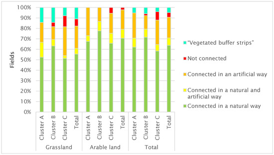
Figure 4.
Proportions of the assessed connectivity types among the mapped clusters and agricultural land use types. The results indicate a rather low overall variability (“Vegetated buffer strips” can be considered as grassland fields connected in a natural way).
Furthermore, a fifth category was identified and termed “vegetated buffer strips” (VBS). These are grassland fields connected in a natural way and located between arable land and streams showing some of the properties (i.e., dimensions) of “normal” VBS. They are, however, not arable land with VBS but leftovers, which for some reason were not turned into arable land and are not subject to fertiliser restrictions. Their share varies between approximately 10 and 15% among the grassland fields and constitutes roughly 5% of all mapped fields. Moreover, a general comparison of all these results—especially when accounting the mapped “VBS” to grassland fields connected in a natural way—indicates a rather low overall variability.
Due to the assessment of the explanatory details, it was possible to analyse the causes of fields not being connected in a natural way and the different types of artificial connections present in the mapped clusters (Figure 5). Fields categorised as “VBS” were excluded from this analysis. Table 4 shows the causes and their respective shares as identified in the field mapping campaign. These data clearly reveal that road embankments are the main cause of influence on emissions and transport pathways (approx. 65%). They are followed by single storm drains unrelated to roads or roadside ditches and influences stemming from differences between the actual and the mapped stream network (e.g., as a result of cased streams or unknown channels) (both approx. 15%). The remaining almost 10% are composed of a variety of causes including sinks and settlements.
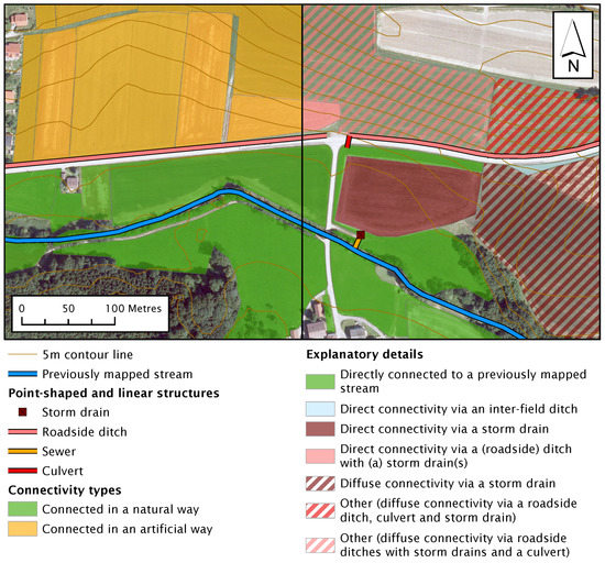
Figure 5.
Exemplified visualisation of some of the results of the field mapping campaign with connectivity types shown on the left and explanatory details on the right side of the figure. The part above connectivity types on the left side of the legend is common to both sides. Please note that the top- and rightmost, bright looking field behind the north arrow does not belong to the mapped cluster.
Table 4.
Causes of influence on emissions and transport pathways expressed as percentage of all influenced fields as well as all mapped fields.
Considering all mapped fields, road embankments with subsurface drainage (i.e., storm drains at varying distances along road embankments often in combination with roadside ditches) are responsible for influencing emissions and transport pathways of almost a quarter of the fields. Given that about 45% of the mapped fields are subject to an influence, road embankments with subsurface drainage account for approximately half of all influences present in the mapped clusters. They furthermore constitute about 80% of the fields influenced by road embankments.
3.2. Impact of Storm Drains at Road Embankments on PP Transport
The calibration quality of the six modelled scenarios (two road and three transport coefficient scenarios) indicates good model performance (cf., [56]) and is consistent across all scenarios (Table 3). Unfortunately, a validation with independent river loads could not be performed, since not all of the input data are available at the same spatial resolution in another period of time.
The plausibility check of the chosen PP transfer coefficients in roadside ditches utilising the estimated PP retention per metre roadside ditch range demonstrates that a transfer coefficient of 0.6 fits best with both road scenarios. Whereas a transfer coefficient of 0.8 scrapes at the lower limit of the estimated PP retention per metre roadside ditch range in both instances, a transfer coefficient of 0.4 only scrapes at the upper limit of the major road scenario and indicates that the best fit actually seems to be somewhere between a transfer coefficient of 0.5 and 0.6 in the other case.
A comparison of the modelled shares of storm drains at road embankments on total PP emissions between the six modelled scenarios results in a small range of 8 to 14% for the major roads scenarios and a big range of 27 to 44% for the scenarios considering all roads. Overall, the range encompasses a share of as little as approximately one tenth and as much as almost one half.
3.3. Best Estimate of the Overall Impact of Storm Drains at Road Embankments on Diffuse PP Emissions
Overall, the retention rate as calculated by the extended PhosFate model fits well to real world data. By comparing the values of the transfer coefficients and the resulting mean estimated PP transfer ratios in roadside ditches, it can be concluded that a transfer coefficient of 0.6 fits best and is therefore the most likely coefficient. However, neither the major roads nor the all roads scenario seems to appropriately reflect the situation in the case study catchment.
According to the results of the Bayesian model, the mode of the share of road embankments with subsurface drainage on all road embankments is 77% and the equal-tailed 95% credible interval ranges from 20 to 98%. While this is quite a big range, the 90% HPDI ranges from 54 to 100% only. Taking into account that the case study catchment appears all in all fairly homogeneous, our best estimate of the share of storm drains at road embankments on total PP emissions consequently ranges from about one fifth to one third. This estimate was obtained by combining the 90% HPDI with the PhosFate results of the all roads scenario with a transfer coefficient of 0.6.
4. Discussion
By applying the mapping key presented here, it could be shown that it is capable of collecting valuable information on agricultural and civil engineering structures potentially influencing emissions and transport pathways in agricultural catchments. It clearly revealed that the main influencing factor in the mapped clusters are road embankments with subsurface drainage and that the most important question in this case study catchment is whether a road embankment is equipped with one or more storm drains or not.
A limitation of the mapping key is that it is adequate to assess structural but not functional elements of connectivity. It thus only points out potential connectivity [34]. This, however, fits well to spatially distributed models like PhosFate, which incorporate the (R)USLE, as this equation only estimates an (erosion) potential as well. Beyond that, due to the involvement of parameters for the calculation of the hydraulic radius related to discharge frequency, PhosFate again calculates a (transport) potential only. This calculation of mere potentials can be considered a limitation of the chosen modelling approach, which otherwise shows a good ratio of model performance to data requirements (cf., [4]).
Calibrating PhosFate on several water quality gauges along the main river of the case study catchment ensured that the utilised input data reflect the spatial distribution of the relevant transport pathways and that the assumption of global calibration parameters was justified. The fact that all modelled scenarios show an equally good calibration quality further supports this.
When interpreting the channel and in particular the field deposition rate resulting from calibration, one has to bear in mind, though, that they include a temporal component. This means that apart from integrating catchment properties influencing transport (e.g., density and average width of hedges as well as reins not covered by the land use input data), they also relate the local modelled mean annual transport loads corresponding to the chosen discharge frequency of the hydraulic radius to the global observed mean annual loads at water quality gauges. In other words, they at least partly control whether a certain area contributes to the overall river load (i.e., becomes connected) or not (cf., [63]).
Another limitation of the mapping key is its use of discrete mapping units. For one thing, they are of different sizes, for another, due to potential flow routing from one unit to another, not all of them may be statistically independent. The latter can be solved by delineating zero-order catchments and using these as mapping units.
Addressing the issue of different sizes is more challenging. In fact, assuming an equal-sized sampling grid at a spatial resolution smaller than the average field size would increase the issue of dependent samples, whereas a sampling grid at a spatial resolution larger than the average field size would lead to ambiguity. This already is a problem with fields (e.g., same field on both sides of a ridge) and means that a certain property is sometimes only valid for the majority but not all of the assessed area.
Getting back to zero-order catchments, though, and assuming that the sizes of those (parts) showing a certain property and those not showing a certain property average out in a sampling cluster (i.e., small sub-catchment in this case), this issue can probably be neglected, as the weights stay the same in both cases. This would even allow for a geostatistical approach, interpolating ratios between clusters [64]. The total number of affected units and their associated areas or pollutant loads could then be estimated with the help of auxiliary data.
Ali and Roy [32] compare different spatial sampling schemes and conclude that cyclic sampling is the most adequate sampling design for geostatistical analysis. It should therefore be investigated how and with how much effort it can be successfully applied to cluster sampling within catchment areas of several hundred square kilometres and if the above assumption holds true.
So while the use of fields as mapping units worked well, there may be much precision to gain by switching to zero-order catchments in the future. This, nonetheless, has the complication of many possible statistical populations (cf., [65]), each strongly depending on the type and resolution of elevation data as well as flow routing algorithm used for their delineation. Again, future research should investigate if mapping results are sensitive to these and if it may be advantageous to only consider zero-order catchments with a certain minimum size or showing a certain shape for statistical inference.
Furthermore, another limitation of the chosen modelling approach results from using a global transport coefficient. As storm drains are usually built at locations of high overland flow concentration, it is not unlikely that their locations also exhibit high erosion and in turn high diffuse PP emissions along with steep slopes and short or even no passages through roadside ditches where retention can take place. A global transport coefficient simply considering average conditions may therefore overestimate retention under such conditions. Thus, the overall impact of storm drains at road embankments on diffuse PP emissions may be even higher. This consideration should likewise be subject of future research.
Finally, if one wanted to know the exact locations of, for example, storm drains or culverts, a conceivable solution could be to focus on a narrow strip along roads only. In this case, the question could be formulated as machine learning classification problem for which several existing model types could be utilised (e.g., logistic regression, decision trees, support vector machines and artificial neural networks).
A good start for this might be to use high resolution orthophotos in combination with high resolution airborne topographic Light Detection And Ranging (LiDAR) data as input to learn from. Another possibility would be to equip a car with appropriate sensors and collect topographic LiDAR data including pictures and videos from the roadsides by merely driving along all of them or at least along those of interest [66]. In the light of rather recent advancements in image recognition with deep neural networks (e.g., [67]) and their emerging ability to produce a measure of uncertainty even in the context of large scale image classification problems [68], such a task becomes less and less utopian. To get an idea of what is going on in a catchment area, such detail, however, is usually not required.
5. Conclusions
The influence of road embankments with subsurface drainage can be of importance in catchment areas with a strong tradition towards this drainage type. In case there is indication of this in a certain catchment, a field mapping campaign assessing the degree of their influence should be performed. This is particularly important when trying to identify critical source areas and finding suitable spots for the implementation of measures reducing pollutant emissions into surface waters (cf., [69]).
Field observations capable of collecting valuable information on agricultural and civil engineering structures potentially influencing emissions and transport pathways can already be accomplished with very simple means. Carried out with a mobile GIS application and a simple mapping key as the one presented in this study, they can easily be integrated into the preparation of modelling studies aiming at the identification of critical source areas at catchment scale. In the end, the combination and comparison of field observations with simplifying hypothesis [70] and model output [71,72] proved to be of great help in assessing the impact of agricultural and civil engineering structures in this case study catchment.
Author Contributions
Conceptualization, G.H. and M.Z.; Data curation, G.H.; Formal analysis, G.H.; Funding acquisition, M.Z.; Methodology, G.H.; Project administration, M.Z.; Supervision, M.Z.; Visualization, G.H.; Writing—original draft, G.H.; Writing—review & editing, M.Z.
Funding
This research was funded by the State Government of Upper Austria contract numbers AUWR-2012- 61484/46-StU and AUWR-2015-231931/24-StU.
Acknowledgments
The authors especially thank Franz Überwimmer and Ulrike Steinmair of the State Government of Upper Austria for hosting constructive discussions of the results. Furthermore, our thank goes to Markus Langer, Andreas Lechner and Helene Trautvetter for carrying out the field mapping campaign as well as to Ottavia Zoboli and Arabel Amann for their valuable help in improving the manuscript.
Conflicts of Interest
The authors declare no conflict of interest.
Appendix A. Mapping Key Tables
Table A1.
Connected or not in a natural way. Mosimann et al. [33] acknowledge obstacles higher than 50 as effective barriers for surface runoff, preventing connectivity, and so do we.
Table A1.
Connected or not in a natural way. Mosimann et al. [33] acknowledge obstacles higher than 50 as effective barriers for surface runoff, preventing connectivity, and so do we.
| Code | Description |
|---|---|
| 0 | Not connected in a natural way |
| 1 | Connected in a natural way |
Table A2.
Explanatory details for mapping units not connected in a natural way. Particularly code 4 and 5 in combination with the codes of Table A3 can also be used to indicate a change in connectivity (e.g., a change from direct towards diffuse connectivity).
Table A2.
Explanatory details for mapping units not connected in a natural way. Particularly code 4 and 5 in combination with the codes of Table A3 can also be used to indicate a change in connectivity (e.g., a change from direct towards diffuse connectivity).
| Code | Description |
|---|---|
| 1 | Road embankment |
| 2 | Levee or other linear structure |
| 3 | Depression |
| 4 | Previously mapped stream is missing |
| 5 | Previously mapped stream is cased |
| 99 | Other |
Table A3.
Explanatory details for mapping units connected in a natural way.
Table A3.
Explanatory details for mapping units connected in a natural way.
| Code | Description |
|---|---|
| 1 | Directly connected to a previously mapped stream |
| 2 | Direct connectivity via a previously unknown channel |
| 3 | Direct connectivity via a gully |
| 4 | Diffuse connectivity |
| 99 | Other |
Table A4.
Artificial connection.
Table A4.
Artificial connection.
| Code | Description |
|---|---|
| 0 | Not present |
| 1 | Present |
| 2 | Diffusely present in a downstream mapping unit |
Table A5.
Explanatory details for mapping units connected in an artificial way. Diffuse connectivity in this context means that an artificial connection is either diffusely present in a downstream mapping unit (see code 2 of Table A4) or that an artificial structure is not directly connected to a surface water (e.g., a ditch ending in a forest).
| Code | Description |
|---|---|
| 1 | Direct connectivity via an inter-field ditch |
| 2 | Direct connectivity via a roadside ditch |
| 3 | Direct connectivity via a storm drain |
| 4 | Direct connectivity via a culvert |
| 5 | Direct connectivity via a (roadside) ditch with (a) storm drain(s) |
| 6 | Direct connectivity via a (roadside) ditch with (a) culvert(s) |
| 7 | Diffuse connectivity via an inter-field ditch |
| 8 | Diffuse connectivity via a roadside ditch |
| 9 | Diffuse connectivity via a storm drain |
| 10 | Diffuse connectivity via a culvert |
| 11 | Diffuse connectivity via a (roadside) ditch with (a) storm drain(s) |
| 12 | Diffuse connectivity via a (roadside) ditch with (a) culvert(s) |
| 99 | Other |
Table A6.
Presence and absence of natural features as well as artificial point-shaped and linear structures.
Table A6.
Presence and absence of natural features as well as artificial point-shaped and linear structures.
| Code | Description |
|---|---|
| 1 | Channel |
| 2 | Gully |
| 3 | Inter-field ditch |
| 4 | Roadside ditch |
| 5 | Storm drain |
| 6 | Sewer |
| 7 | Culvert |
| 8 | Stream casing |
| 9 | Missing, previously mapped stream |
| 99 | Other |
References
- Heathwaite, A.L.; Quinn, P.F.; Hewett, C.J.M. Modelling and Managing Critical Source Areas of Diffuse Pollution from Agricultural Land Using Flow Connectivity Simulation. J. Hydrol. 2005, 304, 446–461. [Google Scholar] [CrossRef]
- Pionke, H.B.; Gburek, W.J.; Sharpley, A.N. Critical Source Area Controls on Water Quality in an Agricultural Watershed Located in the Chesapeake Basin. Ecol. Eng. 2000, 14, 325–335. [Google Scholar] [CrossRef]
- Strauss, P.; Leone, A.; Ripa, M.N.; Turpin, N.; Lescot, J.M.; Laplana, R. Using Critical Source Areas for Targeting Cost-Effective Best Management Practices to Mitigate Phosphorus and Sediment Transfer at the Watershed Scale. Soil Use Manag. 2007, 23, 144–153. [Google Scholar] [CrossRef]
- De Vente, J.; Poesen, J.; Verstraeten, G.; Govers, G.; Vanmaercke, M.; Van Rompaey, A.; Arabkhedri, M.; Boix-Fayos, C. Predicting Soil Erosion and Sediment Yield at Regional Scales: Where Do We Stand? Earth Sci. Rev. 2013, 127, 16–29. [Google Scholar] [CrossRef]
- Jetten, V.; Govers, G.; Hessel, R. Erosion Models: Quality of Spatial Predictions. Hydrol. Process. 2003, 17, 887–900. [Google Scholar] [CrossRef]
- Forman, R.T.T.; Alexander, L.E. Roads and Their Major Ecological Effects. Annu. Rev. Ecol. Syst. 1998, 29, 207–231. [Google Scholar] [CrossRef]
- Aurousseau, P.; Gascuel-Odoux, C.; Squividant, H.; Trepos, R.; Tortrat, F.; Cordier, M.O. A Plot Drainage Network as a Conceptual Tool for the Spatial Representation of Surface Flow Pathways in Agricultural Catchments. Comput. Geosci. 2009, 35, 276–288. [Google Scholar] [CrossRef]
- Van Oost, K.; Govers, G.; Desmet, P. Evaluating the Effects of Changes in Landscape Structure on Soil Erosion by Water and Tillage. Landsc. Ecol. 2000, 15, 577–589. [Google Scholar] [CrossRef]
- Alder, S.; Prasuhn, V.; Liniger, H.; Herweg, K.; Hurni, H.; Candinas, A.; Gujer, H.U. A High-Resolution Map of Direct and Indirect Connectivity of Erosion Risk Areas to Surface Waters in Switzerland—A Risk Assessment Tool for Planning and Policy-Making. Land Use Policy 2015, 48, 236–249. [Google Scholar] [CrossRef]
- Croke, J.; Mockler, S.; Fogarty, P.; Takken, I. Sediment Concentration Changes in Runoff Pathways from a Forest Road Network and the Resultant Spatial Pattern of Catchment Connectivity. Geomorphology 2005, 68, 257–268. [Google Scholar] [CrossRef]
- Doppler, T.; Camenzuli, L.; Hirzel, G.; Krauss, M.; Lück, A.; Stamm, C. Spatial Variability of Herbicide Mobilisation and Transport at Catchment Scale: Insights from a Field Experiment. Hydrol. Earth Syst. Sci. 2012, 16, 1947–1967. [Google Scholar] [CrossRef]
- Hösl, R.; Strauss, P.; Glade, T. Man-Made Linear Flow Paths at Catchment Scale: Identification, Factors and Consequences for the Efficiency of Vegetated Filter Strips. Landsc. Urban Plan. 2012, 104, 245–252. [Google Scholar] [CrossRef]
- La Marche, J.L.; Lettenmaier, D.P. Effects of Forest Roads on Flood Flows in the Deschutes River, Washington. Earth Surf. Process. Landforms 2001, 26, 115–134. [Google Scholar] [CrossRef]
- Wemple, B.C.; Jones, J.A.; Grant, G.E. Channel Network Extension by Logging Roads in Two Basins, Western Cascades, Oregon. J. Am. Water Resour. Assoc. 1996, 32, 1195–1207. [Google Scholar] [CrossRef]
- Moussa, R.; Voltz, M.; Andrieux, P. Effects of the Spatial Organization of Agricultural Management on the Hydrological Behaviour of a Farmed Catchment during Flood Events. Hydrol. Process. 2002, 16, 393–412. [Google Scholar] [CrossRef]
- Fiener, P.; Auerswald, K.; Van Oost, K. Spatio-Temporal Patterns in Land Use and Management Affecting Surface Runoff Response of Agricultural Catchments—A Review. Earth Sci. Rev. 2011, 106, 92–104. [Google Scholar] [CrossRef]
- Van Rompaey, A.J.J.; Verstraeten, G.; Van Oost, K.; Govers, G.; Poesen, J. Modelling Mean Annual Sediment Yield Using a Distributed Approach. Earth Surf. Process. Landforms 2001, 26, 1221–1236. [Google Scholar] [CrossRef]
- Verstraeten, G.; Van Oost, K.; Van Rompaey, A.; Poesen, J.; Govers, G. Evaluating an Integrated Approach to Catchment Management to Reduce Soil Loss and Sediment Pollution through Modelling. Soil Use Manag. 2002, 18, 386–394. [Google Scholar] [CrossRef]
- Duke, G.D.; Kienzle, S.W.; Johnson, D.L.; Byrne, J.M. Improving Overland Flow Routing by Incorporating Ancillary Road Data into Digital Elevation Models. J. Spat. Hydrol. 2003, 3, 23–49. [Google Scholar]
- Duke, G.D.; Kienzle, S.W.; Johnson, D.L.; Byrne, J.M. Incorporating Ancillary Data to Refine Anthropogenically Modified Overland Flow Paths. Hydrol. Process. 2006, 20, 1827–1843. [Google Scholar] [CrossRef]
- Gramlich, A.; Stoll, S.; Stamm, C.; Walter, T.; Prasuhn, V. Effects of Artificial Land Drainage on Hydrology, Nutrient and Pesticide Fluxes from Agricultural Fields—A Review. Agric. Ecosyst. Environ. 2018, 266, 84–99. [Google Scholar] [CrossRef]
- Kovacs, A.S.; Honti, M.; Clement, A. Design of Best Management Practice Applications for Diffuse Phosphorus Pollution Using Interactive GIS. Water Sci. Technol. 2008, 57, 1727–1733. [Google Scholar] [CrossRef] [PubMed]
- Kovacs, A.; Honti, M.; Zessner, M.; Eder, A.; Clement, A.; Blöschl, G. Identification of Phosphorus Emission Hotspots in Agricultural Catchments. Sci. Total Environ. 2012, 433, 74–88. [Google Scholar] [CrossRef] [PubMed]
- Kovacs, A. Quantification of Diffuse Phosphorous Inputs into Surface Water Systems. Ph.D. Thesis, Technische Universität Wien, Vienna, Austria, 2013. [Google Scholar]
- Zessner, M.; Hepp, G.; Kuderna, M.; Weinberger, C.; Gabriel, O.; Windhofer, G. Konzipierung und Ausrichtung übergeordneter strategischer Maßnahmen zur Reduktion von Nährstoffeinträgen in oberösterreichische Fließgewässer; Technical Report; Amt der Oberösterreichischen Landesregierung: Wien, Austria, 2014.
- Verstraeten, G.; Poesen, J.; Gillijns, K.; Govers, G. The Use of Riparian Vegetated Filter Strips to Reduce River Sediment Loads: An Overestimated Control Measure? Hydrol. Process. 2006, 20, 4259–4267. [Google Scholar] [CrossRef]
- Gascuel-Odoux, C.; Aurousseau, P.; Doray, T.; Squividant, H.; Macary, F.; Uny, D.; Grimaldi, C. Incorporating Landscape Features to Obtain an Object-Oriented Landscape Drainage Network Representing the Connectivity of Surface Flow Pathways over Rural Catchments. Hydrol. Process. 2011, 25, 3625–3636. [Google Scholar] [CrossRef]
- Djodjic, F.; Villa, A. Distributed, High-Resolution Modelling of Critical Source Areas for Erosion and Phosphorus Losses. AMBIO 2015, 44, 241–251. [Google Scholar] [CrossRef]
- Bug, J.F. Modellierung der linearen Erosion und des Risikos von Partikeleinträgen in Gewässer. Ph.D. Thesis, Leibniz Universität Hannover, Hannover, Germany, 2011. [Google Scholar]
- Zessner, M.; Gabriel, O.; Kovacs, A.; Kuderna, M.; Schilling, C.; Hochedlinger, G.; Windhofer, G. Analyse der Nährstoffströme in oberösterreichischen Einzugsgebieten nach unterschiedlichen Eintragspfaden für strategische Planungen (Nährstoffströme Oberösterreich); Technical Report; Amt der Oberösterreichischen Landesregierung: Wien, Austria, 2011.
- BMLFUW. Hydrografisches Jahrbuch von Österreich 2013. Daten und Auswertungen; Technical Report 121; Bundesministerium für Land- und Forstwirtschaft, Umwelt und Wasserwirtschaft: Wien, Austria, 2015.
- Ali, G.A.; Roy, A.G. Revisiting Hydrologic Sampling Strategies for an Accurate Assessment of Hydrologic Connectivity in Humid Temperate Systems. Geogr. Compass 2009, 3, 350–374. [Google Scholar] [CrossRef]
- Mosimann, T.; Backhaus, J.; Westphal, H. Gewässeranschluss von Ackerflächen. Ein Schlüssel für Betriebsleiter und Berater in Niedersachsen; Landwirtschaftskammer Niedersachsen: Hannover, Germany, 2007. [Google Scholar]
- Bracken, L.J.; Wainwright, J.; Ali, G.A.; Tetzlaff, D.; Smith, M.W.; Reaney, S.M.; Roy, A.G. Concepts of Hydrological Connectivity: Research Approaches, Pathways and Future Agendas. Earth Sci. Rev. 2013, 119, 17–34. [Google Scholar] [CrossRef]
- Bracken, L.J.; Croke, J. The Concept of Hydrological Connectivity and Its Contribution to Understanding Runoff-Dominated Geomorphic Systems. Hydrol. Process. 2007, 21, 1749–1763. [Google Scholar] [CrossRef]
- Turnbull, L.; Wainwright, J.; Brazier, R.E. A Conceptual Framework for Understanding Semi-Arid Land Degradation: Ecohydrological Interactions across Multiple-Space and Time Scales. Ecohydrology 2008, 1, 23–34. [Google Scholar] [CrossRef]
- Wainwright, J.; Turnbull, L.; Ibrahim, T.G.; Lexartza-Artza, I.; Thornton, S.F.; Brazier, R.E. Linking Environmental Régimes, Space and Time: Interpretations of Structural and Functional Connectivity. Geomorphology 2011, 126, 387–404. [Google Scholar] [CrossRef]
- Renard, K.G.; Foster, G.R.; Weesies, G.A.; McCool, D.K.; Yoder, D.C. Predicting Soil Erosion by Water: A Guide to Conservation Planning with the Revised Universal Soil Loss Equation (RUSLE); Number 703 in Agriculture Handbook; U.S. Government Printing Office: Washington, DC, USA, 1997.
- Schwertmann, U.; Vogl, W.; Kainz, M. Bodenerosion durch Wasser. Vorhersage des Abtrags und Bewertung von Gegenmaßnahmen, 2nd ed.; Ulmer: Stuttgart, Germany, 1987. [Google Scholar]
- Wischmeier, W.H.; Smith, D.D. Predicting Rainfall Erosion Losses. A Guide to Conservation Planning; Number 537 in Agriculture Handbook; U.S. Government Printing Office: Washington, DC, USA, 1978.
- O’Callaghan, J.F.; Mark, D.M. The Extraction of Drainage Networks from Digital Elevation Data. Comput. Vis. Graph. Image Process. 1984, 28, 323–344. [Google Scholar] [CrossRef]
- Hofer, O.; Fahrner, W.; Pavlis-Fronaschitz, G.; Linder, S.; Gmeiner, P. INVEKOS-Datenpool 2014 des BMLFUW. Übersicht über alle im Ordner, Invekosdaten“ enthaltenen Datenbanken mit ausführlicher Tabellenbeschreibung sowie Informationen zu sonstigen verfügbaren Datenbanken; Technical Report; Bundesministerium für Land- und Forstwirtschaft, Umwelt und Wasserwirtschaft: Wien, Austria, 2014.
- Federal Office of Metrology and Surveying. Digitales Landschaftsmodell. Fließende Gewässer. Available online: http://www.bev.gv.at/portal/page?_pageid=713,2847785&_dad=portal&_schema=PORTAL (accessed on 31 August 2015).
- Desmet, P.J.J.; Govers, G. A GIS Procedure for Automatically Calculating the USLE LS Factor on Topographically Complex Landscape Units. J. Soil Water Conserv. 1996, 51, 427–433. [Google Scholar]
- Choi, Y.; Yi, H.; Park, H.D. A New Algorithm for Grid-Based Hydrologic Analysis by Incorporating Stormwater Infrastructure. Comput. Geosci. 2011, 37, 1035–1044. [Google Scholar] [CrossRef]
- Choi, Y. A New Algorithm to Calculate Weighted Flow-Accumulation from a DEM by Considering Surface and Underground Stormwater Infrastructure. Environ. Model. Softw. 2012, 30, 81–91. [Google Scholar] [CrossRef]
- Geoland.at. Intermodales Verkehrsreferenzsystem Österreich (GIP.at); Technical Report; Geodatenverbund der Länder: Wien, Austria, 2016. [Google Scholar]
- Behrendt, H.; Opitz, D. Retention of Nutrients in River Systems: Dependence on Specific Runoff and Hydraulic Load. Hydrobiologia 1999, 410, 111–122. [Google Scholar] [CrossRef]
- Venohr, M.; Hirt, U.; Hofmann, J.; Opitz, D.; Gericke, A.; Wetzig, A.; Ortelbach, K.; Natho, S.; Neumann, F.; Hürdler, J. The Model System MONERIS Version 2.14.1vba; Leibniz-Institute of Freshwater Ecology and Inland Fisheries: Berlin, Germany, 2009. [Google Scholar]
- Zessner, M.; Kovacs, A.; Schilling, C.; Hochedlinger, G.; Gabriel, O.; Natho, S.; Thaler, S.; Windhofer, G. Enhancement of the MONERIS Model for Application in Alpine Catchments in Austria. Int. Rev. Hydrobiol. 2011, 96, 541–560. [Google Scholar] [CrossRef]
- Engman, E.T. Roughness Coefficients for Routing Surface Runoff. J. Irrig. Drain. Eng. 1986, 112, 39–53. [Google Scholar] [CrossRef]
- Zessner, M.; Zoboli, O.; Hepp, G.; Kuderna, M.; Weinberger, C.; Gabriel, O. Shedding Light on Increasing Trends of Phosphorus Concentration in Upper Austrian Rivers. Water 2016, 8, 404. [Google Scholar] [CrossRef]
- Zessner, M.; Hepp, G.; Zoboli, O.; Mollo Manonelles, O.; Kuderna, M.; Weinberger, C.; Gabriel, O. Erstellung und Evaluierung eines Prognosetools zur Quantifizierung von Maßnahmenwirksamkeiten im Bereich der Nährstoffeinträge in oberösterreichische Oberflächengewässer; Technical Report; Amt der Oberösterreichischen Landesregierung: Wien, Austria, 2016.
- Zessner, M.; Hepp, G.; Kuderna, M.; Weinberger, C.; Gabriel, O. Zustandserfassung, Nährstoffentwicklung und Quantifizierung der Maßnahmenwirksamkeiten von ÖPUL 2007 in oberösterreichischen Einzugsgebieten; Technical Report; Amt der Oberösterreichischen Landesregierung: Wien, Austria, 2017.
- Krause, P.; Boyle, D.P.; Bäse, F. Comparison of Different Efficiency Criteria for Hydrological Model Assessment. Adv. Geosci. 2005, 5, 89–97. [Google Scholar] [CrossRef]
- Moriasi, D.N.; Arnold, J.G.; Van Liew, M.W.; Bingner, R.L.; Harmel, R.D.; Veith, T.L. Model Evaluation Guidelines for Systematic Quantification of Accuracy in Watershed Simulations. Trans. ASABE 2007, 50, 885–900. [Google Scholar] [CrossRef]
- Kapfer, S. Jahresbericht 2013—Korrektur. Zustand der Oö. Fließgewässer gem. WRRL; Technical Report; Amt der Oberösterreichischen Landesregierung: Linz, Austria, 2014.
- Zoboli, O.; Viglione, A.; Rechberger, H.; Zessner, M. Impact of Reduced Anthropogenic Emissions and Century Flood on the Phosphorus Stock, Concentrations and Loads in the Upper Danube. Sci. Total Environ. 2015, 518–519, 117–129. [Google Scholar] [CrossRef] [PubMed]
- Gelman, A. Prior Distributions for Variance Parameters in Hierarchical Models (Comment on Article by Browne and Draper). Bayesian Anal. 2006, 1, 515–534. [Google Scholar] [CrossRef]
- Gelman, A.; Jakulin, A.; Pittau, M.G.; Su, Y.S. A Weakly Informative Default Prior Distribution for Logistic and Other Regression Models. Ann. Appl. Stat. 2008, 2, 1360–1383. [Google Scholar] [CrossRef]
- R Core Team. R: A Language and Environment for Statistical Computing; R Core Team: Vienna, Austria, 2016. [Google Scholar]
- Plummer, M. JAGS: A Program for Analysis of Bayesian Graphical Models Using Gibbs Sampling. In Proceedings of the 3rd International Workshop on Distributed Statistical Computing, Vienna, Austria, 20–22 March 2003. [Google Scholar]
- Lane, S.N.; Reaney, S.M.; Heathwaite, A.L. Representation of Landscape Hydrological Connectivity Using a Topographically Driven Surface Flow Index. Water Resour. Res. 2009, 45, W08423. [Google Scholar] [CrossRef]
- Krivoruchko, K.; Gribov, A.; Krause, E. Multivariate Areal Interpolation for Continuous and Count Data. Procedia Environ. Sci. 2011, 3, 14–19. [Google Scholar] [CrossRef]
- Poeppl, R.; Parsons, A. The Geomorphic Cell: A Basis for Studying Connectivity. Earth Surf. Process. Landf. 2018, 43, 1155–1159. [Google Scholar] [CrossRef]
- Holland, D.A.; Pook, C.; Capstick, D.; Hemmings, A. The Topographic Data Deluge—Collecting and Maintaining Data in a 21st Century Mapping Agency. Int. Arch. Photogramm. Remote Sens. Spat. Inf. Sci. 2016, XLI-B4, 727–731. [Google Scholar] [CrossRef]
- He, K.; Zhang, X.; Ren, S.; Sun, J. Deep Residual Learning for Image Recognition. In Proceedings of the CVPR 2015: 28th IEEE Conference on Computer Vision and Pattern Recognition, Boston, MA, USA, 7–12 June 2015. [Google Scholar]
- Heek, J.; Kalchbrenner, N. Bayesian Inference for Large Scale Image Classification. arXiv 2019, arXiv:1908.03491. [Google Scholar]
- Blackwell, M.S.A.; Hogan, D.V.; Maltby, E. The Use of Conventionally and Alternatively Located Buffer Zones for the Removal of Nitrate from Diffuse Agricultural Run-Off. Water Sci. Technol. 1999, 39, 157–164. [Google Scholar] [CrossRef]
- Ludwig, B.; Boiffin, J.; Chadœuf, J.; Auzet, A.V. Hydrological Structure and Erosion Damage Caused by Concentrated Flow in Cultivated Catchments. CATENA 1995, 25, 227–252. [Google Scholar] [CrossRef]
- Jetten, V.; de Roo, A.; Favis-Mortlock, D. Evaluation of Field-Scale and Catchment-Scale Soil Erosion Models. CATENA 1999, 37, 521–541. [Google Scholar] [CrossRef]
- van Dijk, P.M.; Auzet, A.V.; Lemmel, M. Rapid Assessment of Field Erosion and Sediment Transport Pathways in Cultivated Catchments after Heavy Rainfall Events. Earth Surf. Process. Landf. 2005, 30, 169–182. [Google Scholar] [CrossRef]
© 2019 by the authors. Licensee MDPI, Basel, Switzerland. This article is an open access article distributed under the terms and conditions of the Creative Commons Attribution (CC BY) license (http://creativecommons.org/licenses/by/4.0/).