Forecasting Groundwater Level for Soil Landslide Based on a Dynamic Model and Landslide Evolution Pattern

Abstract

The occurrence and migration of groundwater is a key natural factor that directly affects the stability of landslides, and rainfall has a large effect on the groundwater level in soil landslides. This study used the Baijiabao landslide in the Three Georges area of China as the research subject and used a combination of more than seven years of rainfall and GPS (Global Positioning System) monitoring data from 2007 to 2013. We applied the K-means clustering method to classify one cycle of the evolution stage into three classes based on the relative displacement of the main sliding surface of the landslide. To illustrate the relationship between the three landslide evolution divisions and the dynamic indicators, we identified rainfall factors that correspond to the actual change in the landslide using the minimal description length principle method. Based on the relationship between the actual deformation stage of the landslide and the rainfall factor from historical monitoring, the mean absolute error of the dynamic exponential smoothing model was 0.053, and the correlation coefficient was 0.929. The size of the smoothness index could be modified in real-time to achieve dynamic correction, which indicates that the model exhibited high reliability and confirmed the usefulness of the proposed model for forecasting groundwater level changes based on deep-seated soil landslide type.

1. Introduction

Landslides have the characteristics of large loss, a frequent occurrence, widespread regional distribution, and other features [1]. Fluctuations in groundwater levels are an important natural factor that influences the stability of landslides [2]. It has been estimated that more than 90% of soil slope failures are related to rainfall and groundwater [3], and the Landslide groundwater level evolution is controlled by both hydrological and geological factors, which are mainly affected by the rainfall and reservoir water or the temperature. These factors make the groundwater environment a synthetic and nonlinear dynamic system [4]. Rainfall is largely the main groundwater supply source for many landslides; thus, variations in groundwater levels could be estimated based on rainfall monitoring data [5]. Fluctuations in groundwater levels caused by heavy rainfall will continuously influence the stability coefficient of the soft surface of soil landslides in certain areas [6]. Some scholars have established a correlation analysis model for rainfall and groundwater levels and have indirectly estimated the groundwater level trend [7]. The flow of groundwater influences the infiltration (dynamic water pressure) to the deep body of the landslide and then increases the sliding force of the surface [8]. Therefore, predicting dynamic groundwater level changes is critical in the evaluation of landslide stability [9].

Several groundwater level forecasting studies have been conducted for landslide areas as well as other areas. Sangrey et al. [10] applied a numerical simulation model to study groundwater levels based on external factors. Iverson and Major [11] determined seasonal changes in groundwater using a physical interpretation of empirical relations. Cappa et al. [12] determined the slope stability via hydro-mechanical modeling to determine groundwater levels. Unlike other deterministic models, Vallet et al. [13] chose an indirect conceptual model to determine the groundwater level of the Séchilienne landslide. Chen et al. [14] developed a groundwater level forecasting model by combining the theories of self-organizing maps (SOMs) and a radial basis function network (RBFN), and they found that the model could forecast the one-month-ahead groundwater level more precisely than the single-site model. By imputing weekly rainfall, pan evaporation, river stage, and water level in the drain, Mohanty et al. [15] used an artificial neural network (ANN) trained with the Bayesian regularization (BR) algorithm and further predicted groundwater levels two, three, and four weeks ahead in the tube wells of one cluster using the above inputs. From the perspective of spatial analysis, groundwater levels are also subject to seasonal fluctuations [16]. Gundogdu and Guney [17] determined groundwater levels using the universal kriging method in irrigation areas. Due to the close relationship between rainfall and groundwater level, some experts have established correlation analysis models between rainfall and groundwater to predict the tendency of groundwater levels [18] indirectly; thus, this information could be used to reduce the dependence on groundwater monitoring facilities in the context of advanced landslide warnings [19]. For some deep-seated soil landslides, continuous heavy rain may cause large fluctuations in groundwater levels [20], which results in a rapid advancement to the deformation stage. The evolution of groundwater levels in the vicinity of landslides is complicated; rainfall has a hysteresis effect on groundwater levels, and a prediction model derived from static historical data may not reflect the real process timeliness and randomness [21]. At present, most groundwater level forecasting research has been based on the law of historical data by applying data mining approaches, because it is not associated with the actual geological evolution of landslides, mathematical models have poor timeliness and inheritance [22]. Therefore, improving the mathematical precision of these models is important. However, if we consider the influence of nonlinear dynamic factors (e.g., rainfall) on groundwater levels based on the actual evolution process of landslides, the prediction accuracy of groundwater level models may be improved.

In this paper, we use the Baijiabao landslide in the Three Georges area of China as the research subject, which has been categorized as a deep-seated soil and coastal-type landslide. We use the K-means clustering and minimal description length principle (MDLP) methods to extract the relationship between the actual deformation stage of landslides and rainfall factors based on historical monitoring data between 2007 and 2013. Using the temporal changes in the suitable rainfall indicator characteristics, the exponential smoothing model parameters can be dynamically adjusted to respond to the landslide evolution process in real-time; thus, modeling of groundwater level changes in a typical soil landslide can be conducted based on prior knowledge. Furthermore, accuracy tests of the model results were also performed to ensure that this type of model is robust and has extensive practical applications.

2. Theoretical Background

2.1. Quadratic Exponential Smoothing Model

The groundwater level may reflect the stability of a landslide, and changes in future groundwater levels must be predicted. Exponential smoothing is a data processing method, and the weights from this method decline as the temporal scale of the data increasingly differs from that of the forecasting period [23,24]. It is a complicated task to forecast changes in groundwater levels. However, this model has some advantages, such as a short modeling time and limited training data requirements. In some situations, if the data curve exhibits a rising or falling trend, it is better to apply the quadratic, exponential smoothing model, although the basic exponential method may yield a large deviation in the predictions [25]. This model can be used to perform other types of exponential smoothing based on a static parameter. In most cases, only three training data sets and a single parameter are needed to build a predictive model. Groundwater levels change depending on the rainy and dry seasons; therefore, this algorithm can be well adapted to forecasting groundwater fluctuations under certain conditions.

The algorithm can be represented as follows:

V_t⁽¹⁾ = aM_{t − 1} + (1 − a)V_{t − 1}⁽¹⁾

(1)

V_t⁽²⁾ = aV_t⁽¹⁾ + (1 − a)V_{t − 1}⁽²⁾

(2)

All subscripts here indicate the current time or time period, where V_t and V_t−1 stand for the smoothed groundwater levels, and a is a constant, which can be called the smoothing coefficient [26]. M_t−1 is the measured groundwater level, and V_t⁽¹⁾ and V_t⁽²⁾ can be acquired from the training data set; this method could be described as follows:

D_{t + T} = a_t + r_tT

(3)

a_t = 2V_t⁽¹⁾ − V_t⁽²⁾

(4)

r_t = a(V_t⁽¹⁾ − V_t⁽²⁾)/(1 − a)

(5)

In the above three formulas, T is the forecasted stage, D_{t + T} represents the forecasted groundwater level, and a_t and r_t are parameters in the model. Equations (1)–(5) indicate that the smoothing coefficient, or damping coefficient (a) has a large impact on the related calculations, and it may reflect an approximation of the forecasted values based on the available data [27].

2.2. Effect of Smoothness Parameter on the Forecasted Value

In real applications, the smoothness parameter or smoothness coefficient is often used as a static value (from 0 to 1). The predicted values are more closely related to current data when the smoothness coefficient approaches 1, although there is an inherent deviation between the model values based on the available training data. In this case, the data curve will change more sharply than that before the beginning of the steep trend. In contrast, when the smoothness parameter approaches 0, the groundwater level curve is smoother than before and more related to the model values based on the training data. The smoothing parameter can be derived from the results of many cases, and personal expert experience is often used to confirm the values of the smoothness coefficient [28]. In this study, we considered the specific features of soil landslide movements, tried to acquire dynamic smoothness coefficients for different periods, and ultimately obtained a general trend in the groundwater fluctuations of the changing system.

Two methods are often used to represent the forecasting accuracy of a time series model [29]. Namely, the mean absolute error (MAE) and the correlation coefficient (R):

$$\mathrm{MAE}=\frac{1}{\mathrm{n}}{\displaystyle \sum }_{\mathrm{t}=1}^{\mathrm{n}}\left|D\left(t\right)-D^{\prime }\left(t\right)\right|$$

(6)

$$\mathrm{R}={\displaystyle \sum }_{\mathrm{i}=1}^{\mathrm{n}}\left[\left(X_i-X^{\prime }\right)\left(Y_i-Y^{\prime }\right)\right]/\sqrt{{\displaystyle \sum }_{\mathrm{i}=1}^{\mathrm{n}}{\left(X_i-X^{\prime }\right)}^2}\sqrt{{\displaystyle \sum }_{\mathrm{i}=1}^{\mathrm{n}}{\left(Y_i-{\mathrm{Y}}^{\prime }\right)}^2}$$

(7)

In Equations (6) and (7), D(t) represents the actual data, $D^{\prime }\left(t\right)$ is the forecasted value, n is the number of data points, and t represents the interval time of the two data in one adjacent period, which is two months in this paper. X_i represents the actual data, and Y_i represents the forecasted value of the modeling process; $X^{\prime }$ and $Y^{\prime }$ represent the means of the two data types. The lower the MAE is, the lower the model error. Moreover, if R increases, the correlation between the modeled values and actual data increases, indicating an improvement in the model forecasting ability.

2.3. Clustering Analysis

Clustering is a method that can be used to divide a dataset into groups or classes. On the premise of no prior knowledge, this method can automatically group data based on the relative degree of certain characteristics, and the results indicate that the characteristics of individuals in the same group are similar in structure; in contrast, individuals in different groups are less similar [30]. The advantage of having “no prior knowledge” refers to the lack of pre-specified grouping criteria for the clustering analysis, which still has the characteristics of comprehensiveness and objectivity in terms of exploring the internal structure of the data. We applied the K-means method to determine the evolution of soil landslides, and this method facilitated the introduction of dynamic parameters, namely, the dynamic smoothness coefficient.

The K-means clustering process is accomplished by repeatedly moving the cluster center to minimize the total measurement in the cluster [31]. The most commonly used distance calculation method is the Euclidean metric. For example, the Euclidean metric between x and y is the square root of the sum of the difference between the selected variables; thus, the Euclidean metric of two datasets can be defined as follows:

$$d\left(x,y\right)=\sqrt{{\displaystyle \sum }_{i=1}^p{\left(x_i-y_i\right)}^2}$$

(8)

The sample dataset was set as x_i (i = 1, 2,…, N), p represents the value of the N, and it was given a random initial cluster center—c_e (e =1, 2,…, K); it can be specified according to the actual needs. The K-means clustering algorithm alternately performs the following two steps [32]:

(1)

Identify the nearest central point for each sample point X_i:

$$\mathrm{e}=mi{n}_{e\in \left\{1,2,\dots ,K\right\}}d\left(c_e,X_i\right), e=1,2,\dots ,K$$

(9)

(2)

Calculate the means of the samples in each cluster. The mean vector will be the new center:

$$c_e=\frac{1}{n_e}{\displaystyle \sum }_{j=1}^{n_e}{X}_j^{\left(e\right)}, e=1,2,\dots ,K$$

(10)

x_j represents the value in cluster e, and j represents the serial number of the element in one cluster, the number of clustering elements in cluster e was set as n_e. The above two steps are repeated until no samples or very few samples are assigned to different clusters. Note that the K-mean clustering algorithm uses K as the input parameter and divides the collection of N objects into K clusters [33]. Ultimately, the similarity within each cluster is high, and the similarity between different clusters is low. The K-means clustering method generally uses the mean square error as the clustering evaluation criteria; thus, the clustering result exhibits the minimum mean square error (Figure 1).

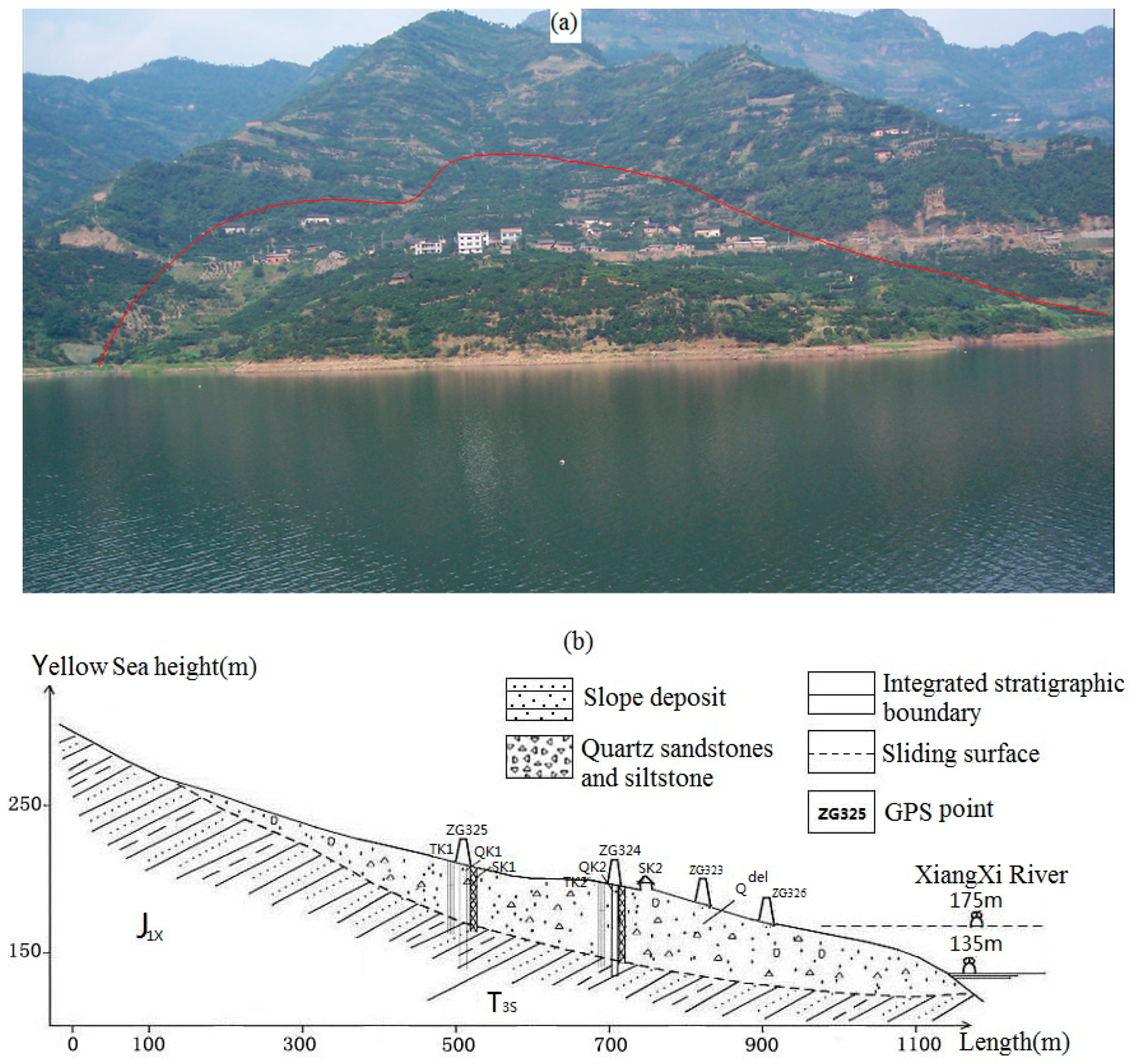
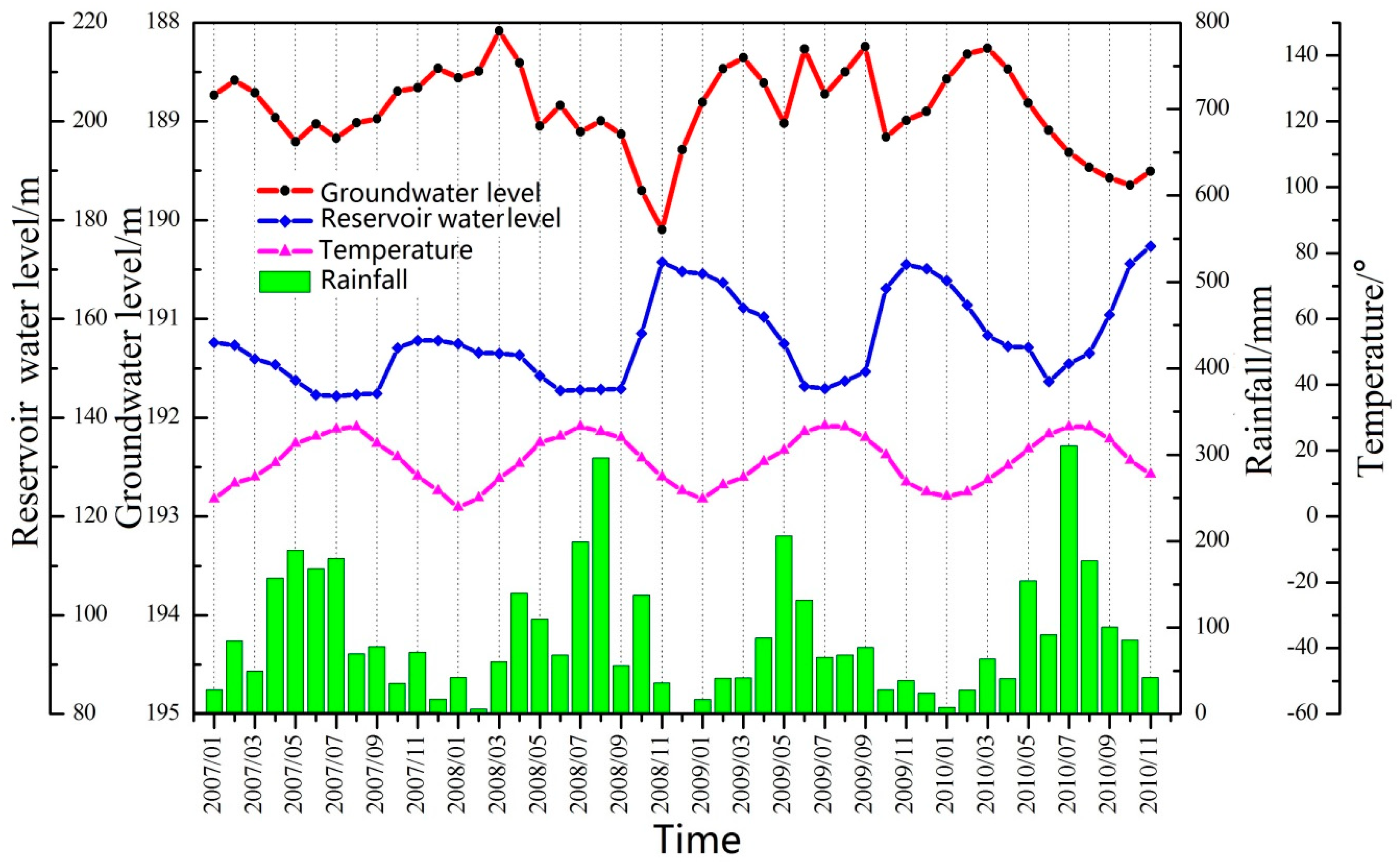
3. Characteristics of Groundwater Level in a Soil Landslide

The Baijiabao landslide is located in Zigui County, Hubei Province, China. It occurred on the right bank of the Xingxi River, which is a tributary of the Yangtze River in the Three Gorges Reservoir (Figure 2a). The landslide area is within a subtropical and monsoon climate belonging to the Three Gorges region. Its sliding interface was a colluvial deposit and underlying bedrock, which formed a relatively water-resistant layer. The maximum sliding direction was from 75° to 85°. The main material of the Baijiabao landslide was composed of crushed stone with silty clay, which was loose and disjointed [34]. The leading edge of the slope was basically submerged in the Xiangxi River, and some landslide bodies become submerged underwater when the reservoir water level reaches 175 m (Figure 2b).

The ZG324 and ZG325 monitoring points were installed in the main sliding zone, and ZG323 and ZG326 were set up in the lower part of the landslide (Figure 2b). During the rainy months (i.e., June to September), as the probability of instability increases, the monitoring frequency is correspondingly increased. The main types of groundwater in the Baijiabao landslide are pore water from loose colluvial deposits, and the slip zone represents the waterproof layer. The groundwater level is mainly affected by rainfall and the reservoir water level; thus, the main source of groundwater is atmospheric rainfall, and the reservoir water is poured into the landslide body when the water level rises. The landslide is located in the Xiangxi River Valley; therefore, its groundwater has the characteristics of on-site recharge and in situ excretion. The groundwater level, reservoir water level, rainfall, and temperature monitoring data are shown in Figure 3.

The landslide is under the monitoring range of the Guizhou rain station in the reservoir area, and the rainfall is reported as the monthly cumulative amount, as shown in Figure 3. From this figure, the groundwater level has a significant relationship with the reservoir water level and rainfall [35]. Considering the effect of the time lag, when rainfall increases or decreases, the groundwater level will also change accordingly within a short time. For example, the accumulated rainfall in July 2010 rose to 301.21 mm, and the groundwater level rose to 189.322 m; however, when the reservoir water level dropped, and the rainfall increased, the rainfall was sufficient to relieve the influence of the reservoir water level, and the groundwater level rose accordingly, e.g., May 2007, May 2008 and May 2009. Rainfall flow into the surface water, and reservoir water becomes the groundwater through infiltration into the landslide body; however, due to the characteristics of the landslide material that influence the permeability of the area, both rainfall and reservoir water have a certain hysteresis effect on the groundwater level. Therefore, when the reservoir water level decreases or rises, and the rainfall decreases or increases, the groundwater level displays a corresponding decrease or increase, and the change was largest in November 2008.

Temperature mainly affects the evaporation of surface water, e.g., as temperature increases, the evaporation capacity of the surface becomes larger, and there is a relatively low amount of surface water in the landslide. However, if the temperature reaches zero or below, the surface freezes, and the amount of surface water infiltration is minimized.

The Baijiabao landslide represents a typical deep-seated soil slope, the material composition of the landslide is very complex, and the standard deviation of the groundwater level data is 18.9, indicating that the fluctuations are very large. The relationship between the groundwater level and its influencing factors is complex and displays a nonlinear response. To minimalize the effect of nonlinearity, groundwater level prediction models are primarily based on external factors [36]. In this study, we chose an environmental factor (rainfall) and physical factors (landslide displacement) to establish a dynamic optimization model to determine the groundwater level changes during the evolution of the soil landslide.

4. Methods

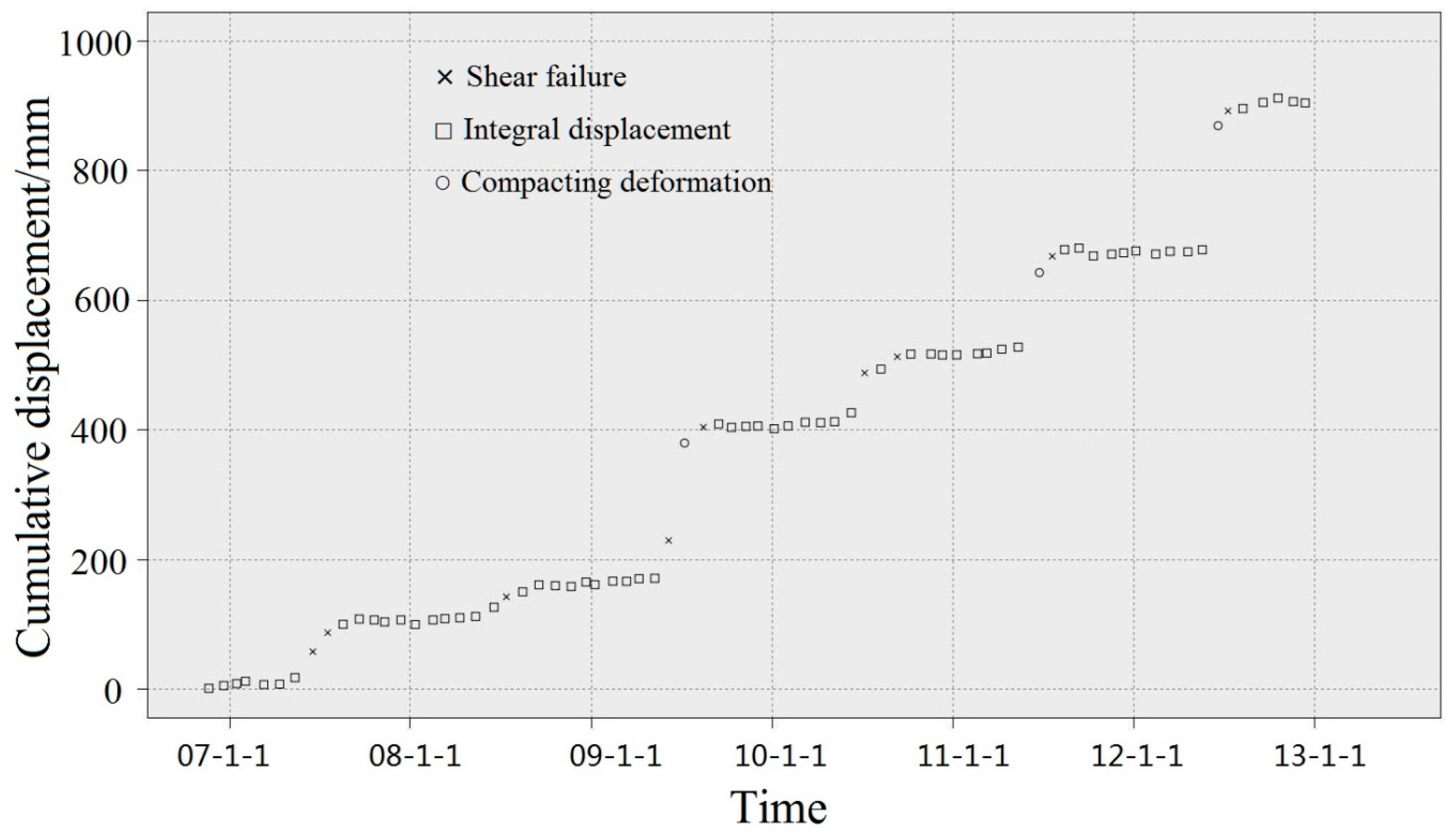
4.1. Division of Landslide Evolution

We used the cumulative displacement of four GPS points in each part of the Baijiabao landslide combined with the monthly rainfall data to obtain a displacement-time scatterplot, as shown in Figure 4.

Important features of the Baijiabao landslide can be ascertained from Figure 4. The data for each GPS point are relatively complete, with no obviously missing values, and the deformation trend of the different monitoring sites is roughly the same. Additionally, the displacement curve has obvious segmentation, periodicity, tendency, and randomness, and it increases during the rainy season from June to September every year. For example, the monthly relative displacement of ZG326 in June 2012 reached 190 mm. With regard to the deformation part, the displacement of the leading edge is not large, and the overall deformation trend is greater than that in the northern part of the landslide. Additionally, relevant research has shown that landslide displacement is related to the evolution stage [37]. The displacement also exhibits three types of changes (i.e., steady rise, steady, and dramatic rise), which could be determined from changes in the slope of the cumulative displacement curve.

In our study, ZG326, a middle trailing edge monitoring site with a large displacement trend and sensitivity to rainfall excretion, was used as the training data to divide the evolution stages of the landslide. We used the K-means clustering method to divide the monthly relative displacement into six initial classes, as described in the following

Table 1. Cluster Similarity.

	C-1	C-2	C-3	C-4	C-5	C-6
C-1	0
C-2	0.02	0
C-3	0.42	0.60	0
C-4	0.70	0.31	0.71	0
C-5	0.24	0.78	0.82	0.53	0
C-6	0.79	0.13	0.53	0.82	0.35	0

¹ C-1 – C-6 represent 6 clustering classes for monthly relative displacement.

.

Many studies have shown that soil landslides progress through a rapid cycle of initial deformation, constant velocity deformation, and acceleration in one phase [38]; moreover, the development of the slope deformation can be divided into three types: compacting deformation, integral displacement, and shear failure. We relied on the cluster similarity of the monthly relative displacement data and the combination of data from clustering-2, clustering-3, and clustering-5 (defined as the shear failure stages), data from clustering-4 and clustering-6 (defined as the integral displacement stage), and data from clustering-1 (used to represent the phase of compacting deformation). Finally, we divided the Baijiabao landslide evolution stages, and the results are shown in Figure 5.

4.2. Establishment of the Dynamic Evaluation Factors

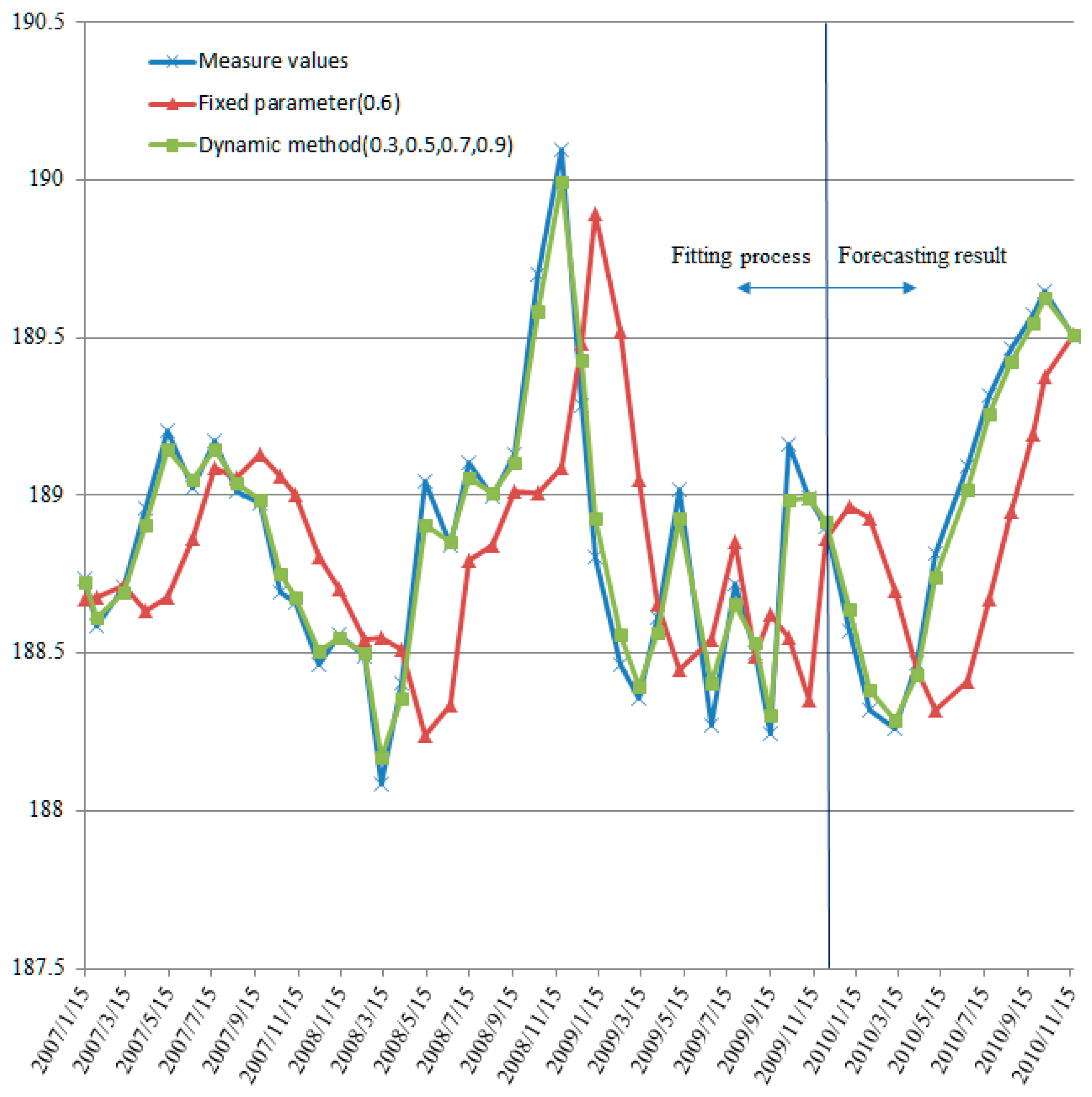
The selection of groundwater level dynamic evaluation factors is critical to the prediction results and can be achieved using a smoothing model. The appropriate factors could reflect the corresponding relationship between the evaluation factors and the groundwater level fluctuations. Based on previous research, rainfall is largely the main groundwater source for some soil landslides. However, we cannot ignore the hysteresis effect of rainfall on groundwater. We considered the use of single parameters used in different stages of landslides and established a dynamic response factor for changing environmental conditions in different deformation stages; thus, we obtained a more accurate model.

In most cases, rainfall indicators are more accessible and reliable than groundwater levels or landslide displacement values due to the robustness of the monitoring instruments. To eliminate the hysteresis effect of rainfall to the groundwater level, we tested three types of rainfall indexes: accumulated monthly rainfall, maximum monthly rainfall, and monthly average rainfall. Based on Equation (6), the correlation coefficients for the three indexes of the deformation stage were determined to be 0.998, 0.827, and 0.447, respectively. In reality, the Baijiabao landslide is relatively loose in terms of its surface structure, and the leading body is submerged in water; thus, the volume of single rainfall events is more likely to form a flood in the river, which results in short-term rainfall having little effect on the groundwater level. As a result, continuous heavy rainfall is an important factor that affects the stability of the Baijiabao landslide and groundwater level fluctuations. From the above analysis, there is no doubt that the accumulated monthly rainfall is more sensitive to groundwater level fluctuations in this typical soil landslide; as a result, we chose this indicator as a dynamic factor for our model.

Based on the discussion in the previous section, we applied dynamic evaluation factors to correspond to the evolution process of landslides. However, the accumulated monthly rainfall is continuous. To illustrate the relationship between the three landslide evolution stages and the selected dynamic indicator, the rainfall data were subjected to a binning operation using the MDLP, and the segmentation results of the accumulated monthly rainfall data are as follows: (3.5–62.1), (62.1–124.1), (124.1–151.1), and (151.1–316). Thus, a relationship between the deformation stage of the landslide and rainfall can be established, and the size of the smoothness index can be modified in real-time to achieve the goal of the model with dynamic correction.

5. Results

As shown in Figure 3, the groundwater level curve exhibits obvious segmentation, periodicity, trend, and randomness features, and the slope of the curve changes significantly during rainy months due to the hysteresis effect of rainfall on the groundwater. Thus, the predicted value should differ substantially from the smoothed trend of the historical data in these periods after the modeling process, which means that the smoothing index parameter of the quadratic, exponential smoothing model should be close to 1. Similarly, the slope of the groundwater level curve should change slightly during periods of little rainfall, which means that the smoothing index parameter should be close to 0. Based on the dynamic evaluation factors established in the last section, the accumulated monthly rainfall data may reflect the different deformation stages of the Baijiabao landslide. Based on the close connection between the rainfall index and the deformation stage of the landslide, we finally applied the results shown in

Table 2. Dynamic Parameters.

Rainfall factor	Stage	Parameter
3.5–62.1	Compacting deformation	0.3
62.1–124.1	Integral displacement	0.5
124.1–151.1	Integral displacement	0.7
151.1–316	Shear failure compaction	0.9

by artificial settings to build dynamic parameters for the groundwater level modeling process.

We dynamically monitored the values of the accumulated monthly rainfall and then chose the appropriate smoothing parameters during the three stages of landslide evolution according to the principles proposed in Table 2. To verify the accuracy of the dynamic exponential smoothing model, we also took the value of 0.6 as the fixed smoothing parameter to generate the comparison model. The groundwater level data from 2007 to 2009 were used as the training sample for the two models, and the values in 2010 were predicted using the models described above. All fitted, forecasted, and measured values are shown in Figure 6.

6. Discussion

The results showed that the fitting and predicted values of the two model types are basically consistent with the measured values, but the model with fixed parameters had a relatively large prediction error at the turning point of the groundwater level change, and there was an obvious hysteresis effect during the whole process. The reason for this effect was that the groundwater system of the landslide is controlled by the physical characteristics of the slope, such as the permeability, which leads to the uncertainty of the main factors affecting the groundwater level. In addition, the turning point often corresponds to sudden changes in the influencing factors, such as rainfall or reservoir water level. The relationship between the actual change in the groundwater level and the model parameters becomes more complicated here, resulting in a relatively large prediction error. For the model with a fixed parameter, the fitting and prediction situation was especially true, e.g., as seen in March 2008. Especially in the period from June to September each year, this soil landslide was more affected by external rainfall, and the fixed-parameter failed to respond to changes in the slope of the groundwater level time series over time; this model value was far from the measured value.

Compared with the observed data, the predicted values generated by the dynamic model were closer to the measured values than those of the exponential smoothing model with a fixed parameter. By classifying the accumulated monthly rainfall, the landslide was divided into three evolution types, and prior knowledge was used to determine the deformation stage and to obtain and set the smoothing parameters of the different processes before modeling. The groundwater level change was represented in real-time by the dynamic method so that the fitted and the forecasted results were significantly improved. The predicted value in 2010 was well correlated with the measured value, which improved the hysteresis effect. The overall accuracy of the two models was evaluated using the mean absolute error and correlation coefficient, and the results are shown in

Table 3. Accuracy evaluation.

Model	Mean Absolute Error	R
Dynamic Fixed	0.053 0.363	0.929 0.327

.

From the previous interpretation of Equations (6) and (7), the evaluation results shown in Table 3, reveal that the dynamic model exhibited a higher degree of fitting and generalization ability than the traditional model, with the error of the former model being approximately six times smaller, and the correlation coefficient increased by approximately a factor of three. The influence of the deep-seated soil landslide dynamic system on the groundwater level was considered; therefore, the varying smoothing parameter values were established in each evolution stage of the landslide; thus, improving the accuracy of the exponential smoothing model. However, due to the influence of the physical properties of the slope on the landslide groundwater system, the prediction error of the dynamic model was relatively large when the influencing factors experienced abrupt changes. Therefore, the influence of the physical properties of the slope in the prediction model warrants attention in future work.

7. Conclusions

The occurrence and migration of groundwater directly affect the stability of soil landslides. The Three Gorges Reservoir area of China experiences a high volume of rainfall, and land surface weathering fissures are common. Thus, atmospheric rainfall recharge is pronounced, and the reservoir water level is high with a well-defined cycle. Therefore, groundwater fluctuations in the reservoir area are very high, and the alternate circulation of groundwater is strong, which is very likely to cause landslides in the coastal parts of the reservoir area. Therefore, predicting dynamic changes in groundwater levels plays a key role in the evaluation of coastal landslide stability.

By referring to the relative displacement of the studied deep-seated soil landslide during an unstable period, the existing theory of three stages of evolution was verified: initial deformation, constant velocity deformation, and acceleration. In this paper, the K-means clustering algorithm was first used to classify the displacement of the main sliding surface of the landslide. Rainfall indicators are more accessible and reliable than groundwater level or landslide displacement data due to the robustness of the monitoring instruments. To illustrate the relationship between the three landslide evolution stages and the rainfall indicator, we implemented a binning operation based on the MDLP method; thus, a relationship between rainfall and the deformation stages was established.

By establishing an association between the model parameters and rainfall classification results, a dynamic exponential smoothing model was used to forecast the groundwater level of the landslide. The MAE and correlation coefficients of the prediction results were 0.053 and 0.929, respectively, which indicated that the model exhibited higher prediction accuracy than the traditional modeling approach. We had established a priori connections with the actual evolution stage of the landslide through the rainfall indicator; hence, the improved model exhibited better fitting and generalization ability than the traditional prediction model, and the proposed model is an effective method for predicting landslide groundwater levels. It should be noted that the prediction error of the model was relatively high when abrupt changes in groundwater level occurred. Therefore, we will combine the physical factors of the landslide itself in the modeling approach to improve the overall accuracy in each deformation stage of a soil landslide in future work.

References

1. Cojean, R.; Cai, Y.J. Analysis and modeling of slope stability in the Three-Gorges Dam reservoir (China)—The case of Huangtupo landslide. J. Mt. Sci. 2011, 8, 166–175. [Google Scholar] [CrossRef]
2. Sun, G.; Zheng, H.; Tang, H.; Dai, F. Huangtupo landslide stability under water level fluctuations of the Three Gorges reservoir. Landslides 2016, 13, 1167–1179. [Google Scholar] [CrossRef]
3. Gattinoni, P. Parametrical landslide modeling for the hydrogeological susceptibility assessment: From the Crati Valley to the Cavallerizzo landslide (Southern Italy). Nat. Hazards 2009, 50, 161–178. [Google Scholar] [CrossRef]
4. Martins-Campina, B.; Huneau, F.; Fabre, R. The Eaux-Bonnes landslide (Western Pyrenees, France): Overview of possible triggering factors with emphasis on the role of groundwater. Environ. Geol. 2008, 55, 397–404. [Google Scholar] [CrossRef]
5. Hong, Y.M.; Wan, S. Forecasting groundwater level fluctuations for rainfall-induced landslide. Nat. Hazards 2011, 57, 167–184. [Google Scholar] [CrossRef]
6. Caris, J.; Van Asch, T. Geophysical, geotechnical and hydrological investigations of a small landslide in the French Alps. Eng. Geol. 1991, 31, 249–276. [Google Scholar] [CrossRef]
7. Bredehoeft, J.D. The water budget myth revisited: Why hydrogeologists model. Ground Water 2002, 40, 340–345. [Google Scholar] [CrossRef]
8. Corominas, J.; Moya, J.; Ledesma, A.; Lloret, A.; Gili, J.A. Prediction of ground displacements and velocities from groundwater level changes at the Vallcebre landslide (Eastern Pyrenees, Spain). Landslides 2005, 2, 83–96. [Google Scholar] [CrossRef]
9. Cascini, L.; Calvello, M.; Grimaldi, G.M. Groundwater Modeling for the Analysis of Active Slow-Moving Landslides. J. Geotech. Geoenviron. Eng. 2010, 136, 1220–1230. [Google Scholar] [CrossRef]
10. Sangrey, D.A.; Harrop-Williams, K.O.; Klaiber, J.A. Predicting Ground-Water Response to Precipitation. J. Geotech. Eng. 1984, 110, 957–975. [Google Scholar] [CrossRef]
11. Iverson, R.M.; Major, J.J. Rainfall, ground-water flow, and seasonal movement at Minor Creek landslide, northwestern California: Physical interpretation of empirical relations. GSA Bull. 1987, 99, 579. [Google Scholar] [CrossRef]
12. Cappa, F.; Guglielmi, Y.; Soukatchoff, V.M.; Mudry, J.; Bertrand, C.; Charmoille, A. Hydromechanical modeling of a large moving rock slope inferred from slope levelling coupled to spring long-term hydrochemical monitoring: Example of the La Clapière landslide (Southern Alps, France). J. Hydrol. 2009, 291, 67–90. [Google Scholar] [CrossRef]
13. Vallet, A.; Bertrand, C.; Mudry, J.; Bogaard, T.; Fabbri, O.; Baudement, C.; Régent, B. Contribution of time-related environmental tracing combined with tracer tests for characterization of a groundwater conceptual model: A case study at the Séchilienne landslide, western Alps (France). Hydrogeol. J. 2015, 23, 1761–1779. [Google Scholar] [CrossRef]
14. Chen, L.-H.; Chen, C.-T.; Pan, Y.-G. Groundwater Level Prediction Using SOM-RBFN Multisite Model. J. Hydrol. Eng. 2010, 15, 624–631. [Google Scholar] [CrossRef]
15. Mohanty, S.; Jha, M.K.; Kumar, A.; Sudheer, K.P. Artificial Neural Network Modeling for Groundwater Level Forecasting in a River Island of Eastern India. Water Resour. Manag. 2010, 24, 1845–1865. [Google Scholar] [CrossRef]
16. Zencich, S.J.; Froend, R.H.; Turner, J.V.; Gailitis, V. Influence of groundwater depth on the seasonal sources of water accessed by Banksia tree species on a shallow, sandy coastal aquifer. Oecologia 2002, 131, 8–19. [Google Scholar] [CrossRef]
17. Gundogdu, K.S.; Guney, I. Spatial analyses of groundwater levels using universal kriging. J. Earth Syst. Sci. 2007, 116, 49–55. [Google Scholar] [CrossRef] [Green Version]
18. Schmertmann, J.H. Estimating Slope Stability Reduction due to Rain Infiltration Mounding. J. Geotech. Geoenviron. Eng. 2006, 132, 1219–1228. [Google Scholar] [CrossRef]
19. Ling, H.I.; Wu, M.-H.; Leshchinsky, D.; Leshchinsky, B. Centrifuge Modeling of Slope Instability. J. Geotech. Geoenviron. Eng. 2009, 135, 758–767. [Google Scholar] [CrossRef]
20. Cho, S.E. Infiltration analysis to evaluate the surficial stability of two-layered slopes considering rainfall characteristics. Eng. Geol. 2009, 105, 32–43. [Google Scholar] [CrossRef]
21. Baker, R. Inter-relations between experimental and computational aspects of slope stability analysis. Int. J. Numer. Anal. Methods Géoméch. 2003, 27, 379–401. [Google Scholar] [CrossRef]
22. Jia, G.; Zhan, T.L.; Chen, Y.; Fredlund, D. Performance of a large-scale slope model subjected to rising and lowering water levels. Eng. Geol. 2009, 106, 92–103. [Google Scholar] [CrossRef]
23. Wood, S.N.; Pya, N.; Säfken, B. Smoothing parameter and model selection for general smooth models. Publ. Am. Stat. Assoc. 2015, 111, 1548–1563. [Google Scholar] [CrossRef]
24. Bermúdez, J.D.; Corberán-Vallet, A.; Vercher, E. Multivariate exponential smoothing: A Bayesian forecast approach based on simulation. Math. Comput. Simul. 2009, 79, 1761–1769. [Google Scholar] [CrossRef]
25. Sbrana, G.; Silvestrini, A. Random switching exponential smoothing and inventory forecasting. Int. J. Prod. Econ. 2014, 156, 283–294. [Google Scholar] [CrossRef]
26. Zhang, W.; Fan, J. Statistical estimation in varying coefficient models. Ann. Stat. 1999, 27, 1491–1518. [Google Scholar] [CrossRef]
27. Kourentzes, N.; Petropoulos, F.; Trapero, J.R. Improving forecasting by estimating time series structural components across multiple frequencies. Int. J. Forecast. 2014, 30, 291–302. [Google Scholar] [CrossRef] [Green Version]
28. Billah, B.; King, M.L.; Snyder, R.D.; Koehler, A.B. Exponential smoothing model selection for forecasting. Int. J. Forecast. 2006, 22, 239–247. [Google Scholar] [CrossRef] [Green Version]
29. Yang, D.; Sharma, V.; Ye, Z.; Lim, L.I.; Zhao, L.; Aryaputera, A.W. Forecasting of global horizontal irradiance by exponential smoothing, using decompositions. Energy 2015, 81, 111–119. [Google Scholar] [CrossRef] [Green Version]
30. Kang, S.H.; Sandberg, B.; Yip, A.M. A regularized k-means and multiphase scale segmentation. Inverse Probl. Imaging 2017, 5, 407–429. [Google Scholar] [CrossRef]
31. Chen, K. On Coresets for k -Median and k -Means Clustering in Metric and Euclidean Spaces and Their Applications. SIAM J. Comput. 2009, 39, 923–947. [Google Scholar] [CrossRef]
32. Chang, H.; Yeung, D.-Y.; Cheung, W.K. Relaxational metric adaptation and its application to semi-supervised clustering and content-based image retrieval. Pattern Recognit. 2006, 39, 1905–1917. [Google Scholar] [CrossRef]
33. Har-Peled, S.; Kushal, A. Smaller Coresets for k-Median and k-Means Clustering. Discret. Comput. Geom. 2007, 37, 3–19. [Google Scholar] [CrossRef]
34. Peng, L.; Xu, S.; Hou, J.; Peng, J. Quantitative risk analysis for landslides: The case of the Three Gorges area, China. Landslides 2015, 12, 943–960. [Google Scholar] [CrossRef]
35. Ilia, I.; Tsangaratos, P. Applying weight of evidence method and sensitivity analysis to produce a landslide susceptibility map. Landslides 2016, 13, 379–397. [Google Scholar] [CrossRef]
36. Shrestha, H.K.; Yatabe, R.; Bhandary, N.P. Groundwater flow modeling for effective implementation of landslide stability enhancement measures—A case of landslide in Shikoku, Japan. Landslides 2008, 5, 281–290. [Google Scholar] [CrossRef]
37. Tang, H.M.; Li, C.D.; Hu, X.L.; Su, A.; Wang, L.; Wu, Y.; Criss, R.; Xiong, C.; Li, Y. Evolution characteristics of the Huangtupo landslide based on in situ tunneling and monitoring. Landslides 2015, 12, 511–521. [Google Scholar] [CrossRef]
38. Dai, F.; Lee, C. Frequency–volume relation and prediction of rainfall-induced landslides. Eng. Geol. 2001, 59, 253–266. [Google Scholar] [CrossRef]
Figure 1. K-means clustering process. (a) Defining the initial three cluster centers, (b) Moving the cluster center to minimize the total mean square error, (c) Forming the final cluster result.
Water 11 02163 g001
Figure 2. Baijiabao landslide geological characteristics: (a) Geological landscape, (b) Profile map of the Baijiabao landslide. The surrounding area of the ground belongs to the Jurassic system.
Water 11 02163 g002
Figure 3. The monitoring data of the reservoir water level, rainfall, temperature, and groundwater level in the Baijiabao landslide.
Water 11 02163 g003
Figure 4. The main GPS (Global Positioning System) monitoring data of the Baijiabao landslide.
Water 11 02163 g004
Figure 5. The deformation stage of the landslide. We use the relative displacement of ZG326 on the main sliding surface to identify each evolution stage: Compacting deformation (0.191 mm–14.132 m), integral displacement (16.122 mm–61.361 mm), and shear failure compaction (114.996 mm–191.358 mm).
Water 11 02163 g005
Figure 6. Modeling result of the groundwater level in Baijiabao landslide (fitted and predicted).
Water 11 02163 g006