WCSPH with Limiting Viscosity for Modeling Landslide Hazard at the Slopes of Artificial Reservoir


Abstract
1. Introduction
2. Numerical Aspects and Mathematical Details
2.1. Mixture Model for Dense Granular Flows
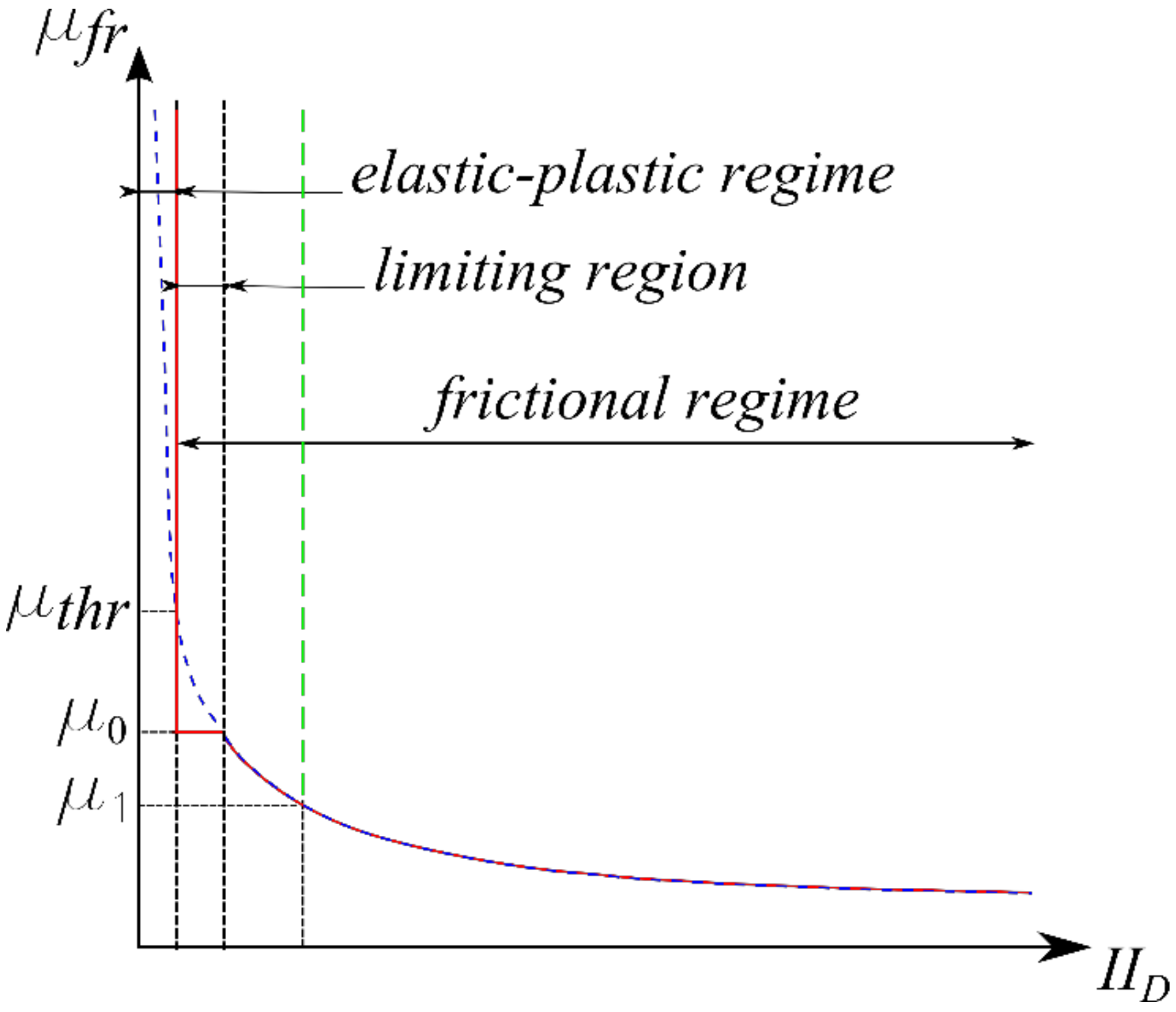
2.2. Implementation of the Limiting Viscosity
3. Numerical Results
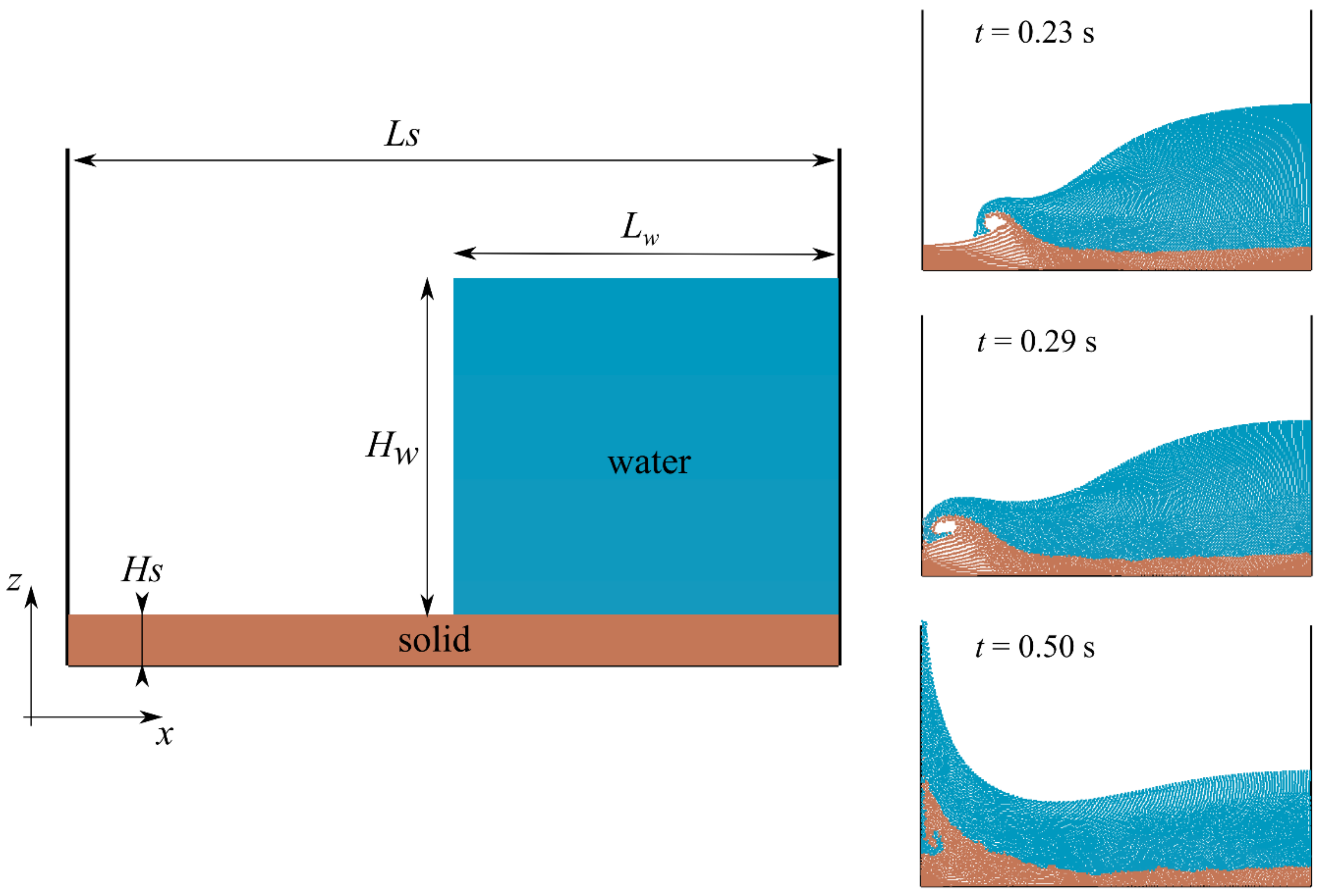
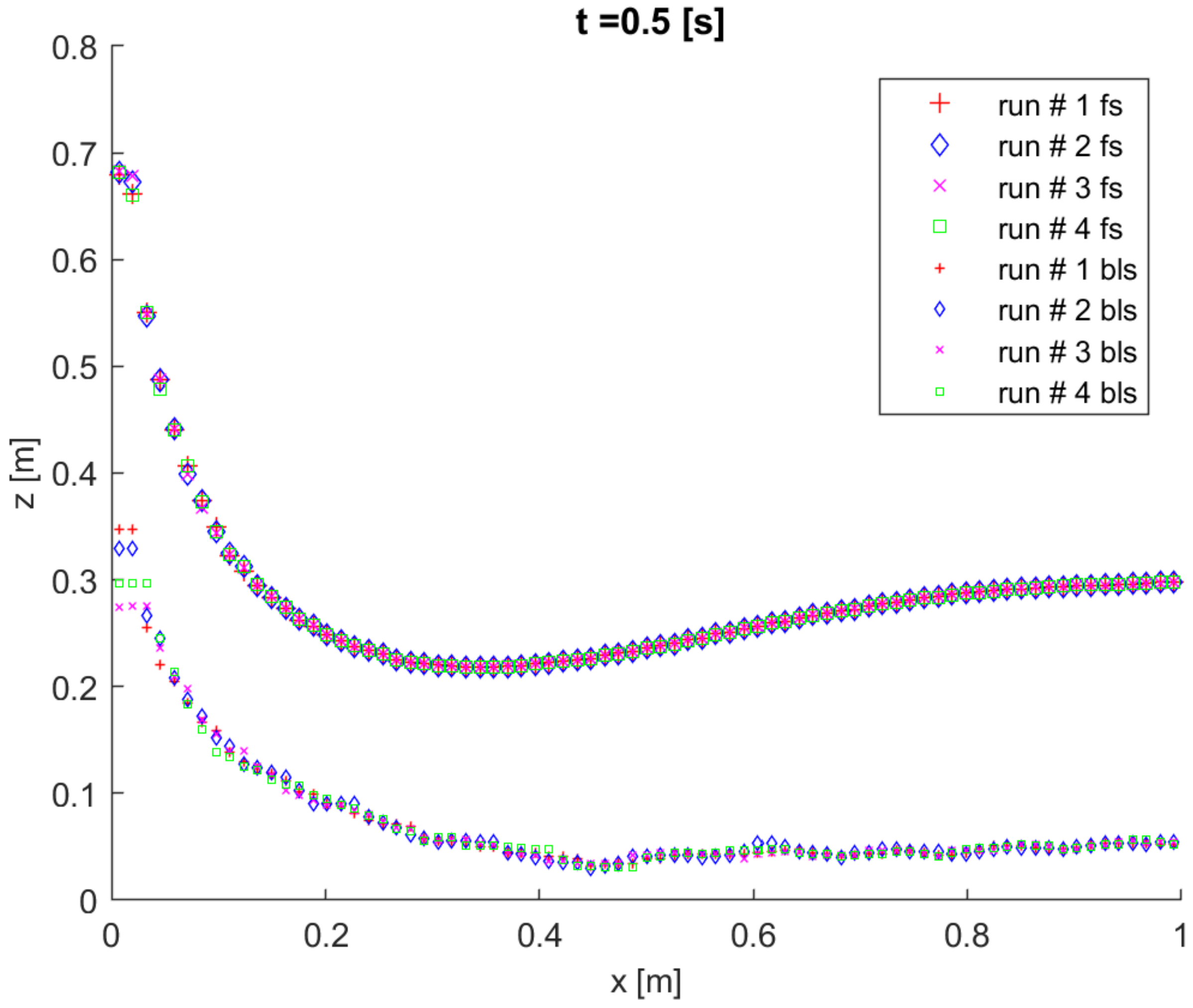
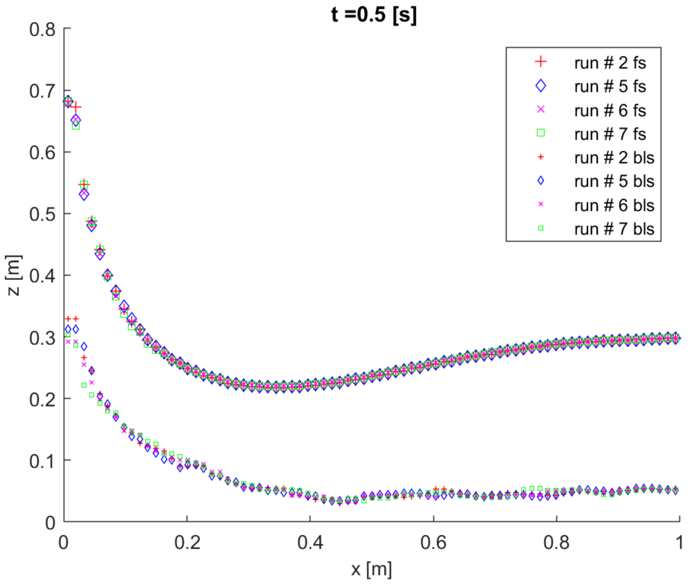
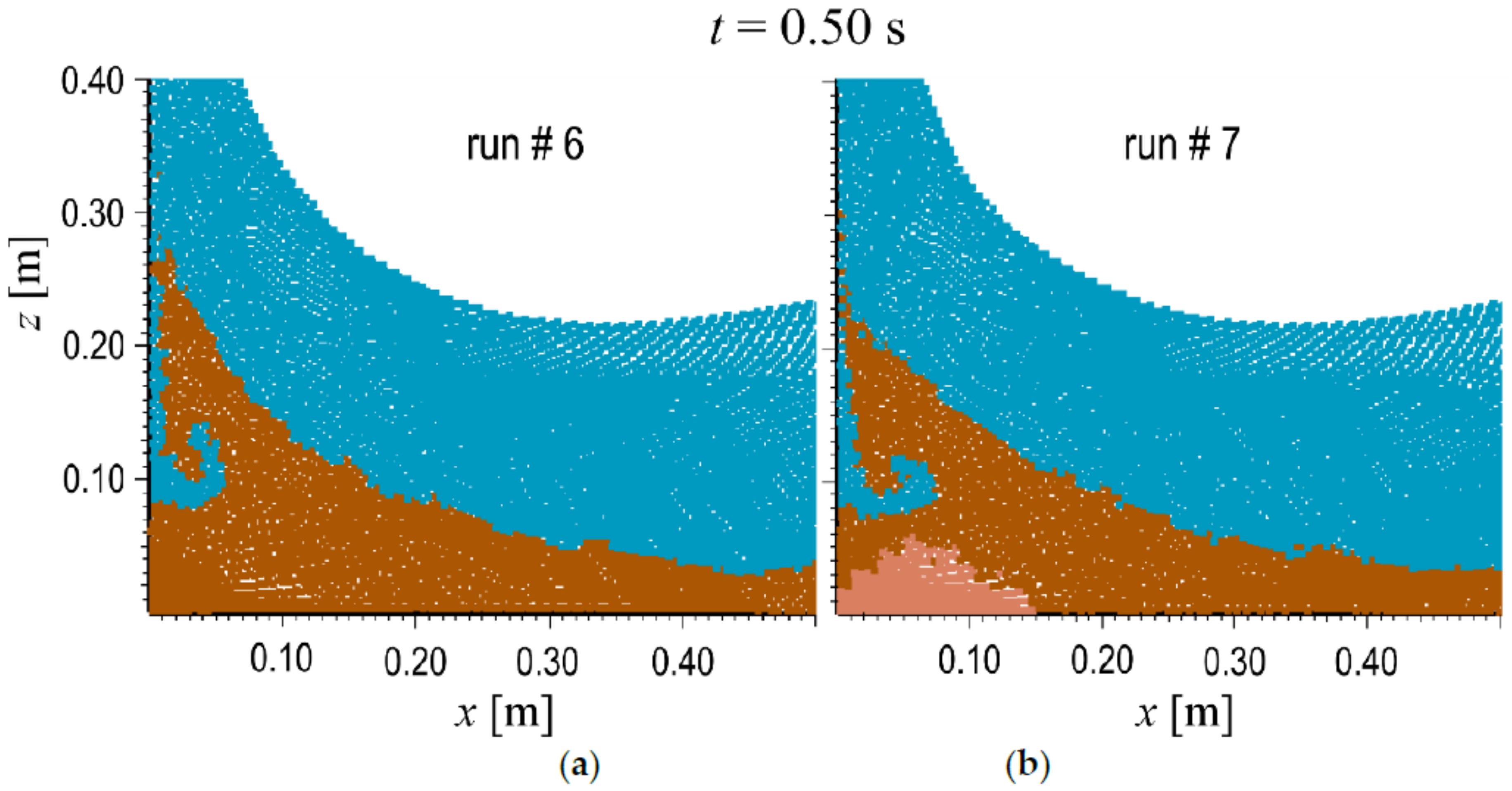
3.1. Two-Dimensional Erosive Dam Break
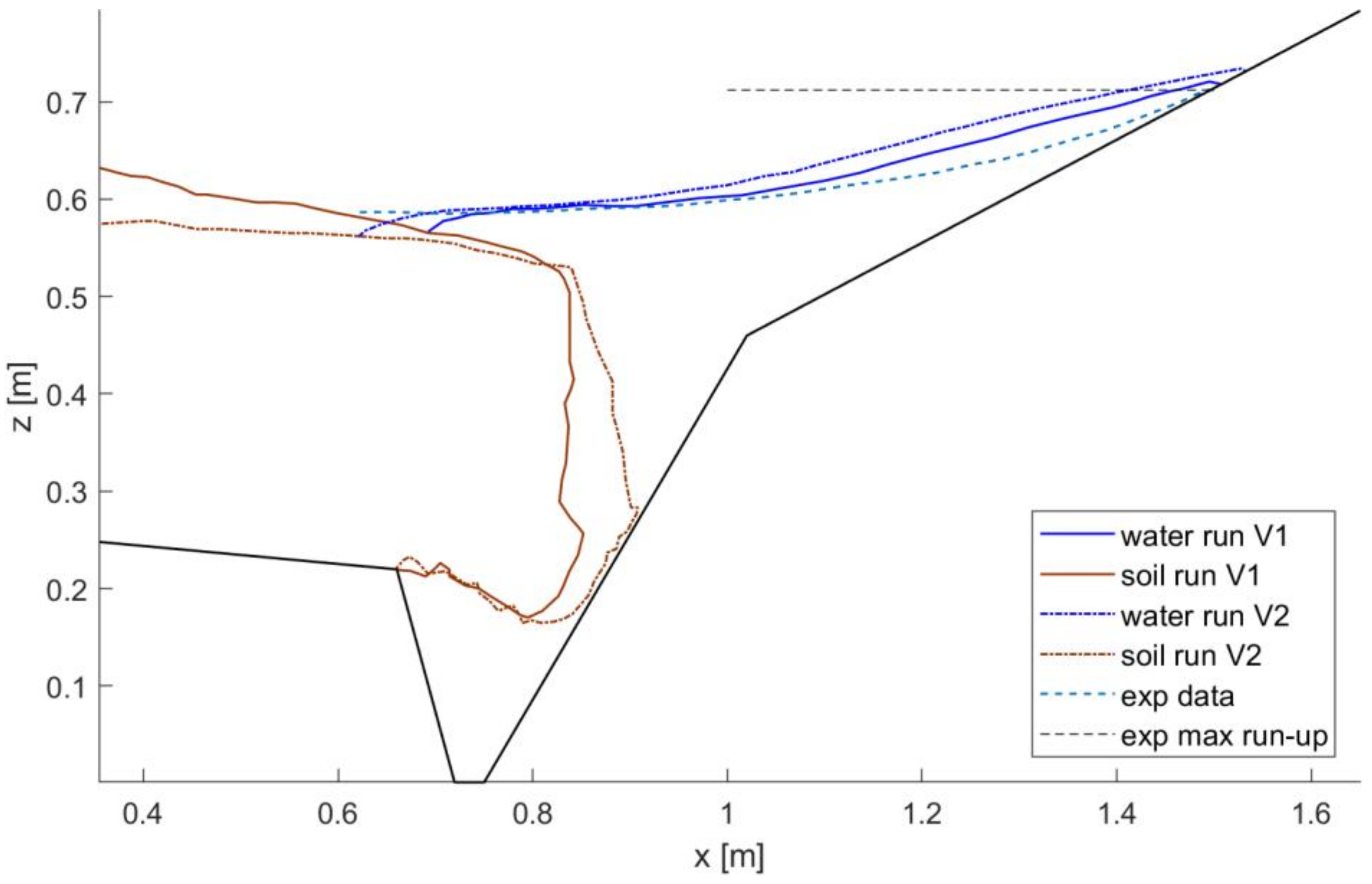
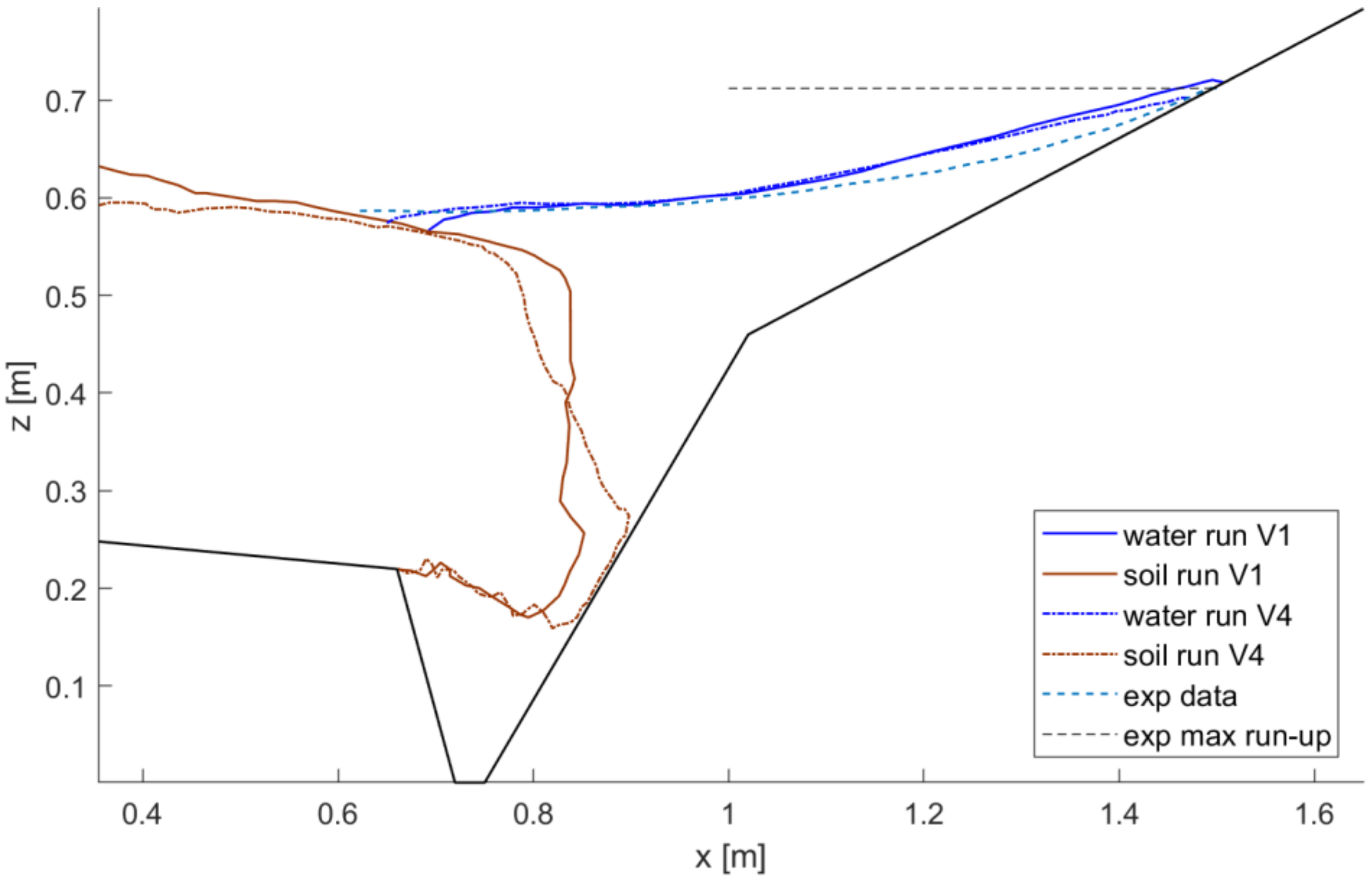
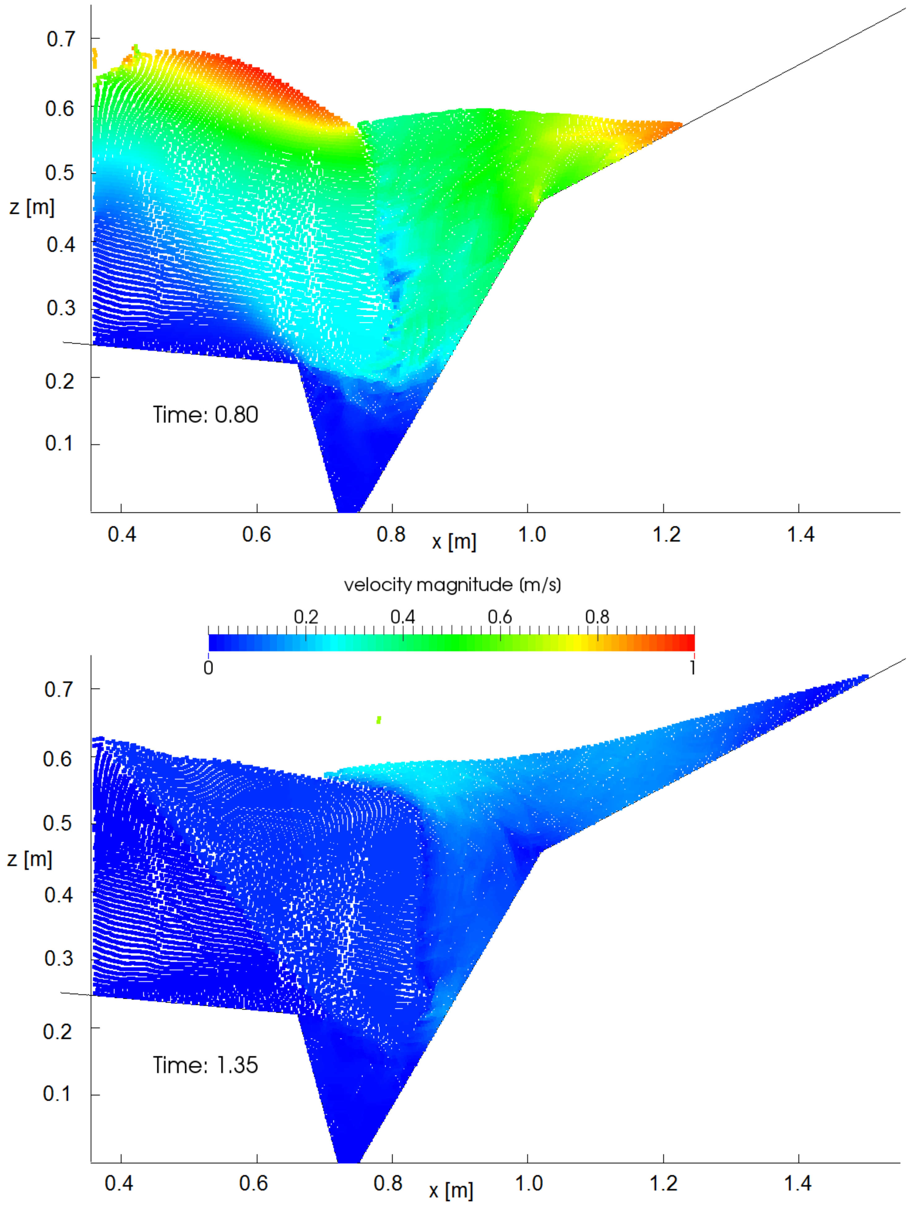
3.2. Validation
4. Conclusions
Acknowledgments
Author Contributions
Conflicts of Interest
References
- Bordoni, M.; Meisina, C.; Valentino, R.; Luc, N.; Bittelli, M.; Chersich, S. Hydrological factors affecting rainfall-induced shallow landslides: From the field monitoring to a simplified slope stability analysis. Eng. Geol. 2015, 193, 19–37. [Google Scholar] [CrossRef]
- Lu, N.; Godt, J. Hillslope Hydrology and Stability; Cambridge University Press: New York, NY, USA, 2013. [Google Scholar]
- Montgomery, D.R.; Dietrich, W.E. A physically based model for the topographic control on shallow landsliding. Water Resour. Res. 1994, 30, 1153–1171. [Google Scholar] [CrossRef]
- Wu, W.; Sidle, R.C. A distributed slope stability model for steep forested basins. Water Resour. Res. 1995, 31, 2097–2110. [Google Scholar] [CrossRef]
- Freeze, R.A. Streamflow generation. Rev. Geophys. 1974, 12, 627–647. [Google Scholar] [CrossRef]
- Iverson, R.M. The physics of debris flows. Rev. Geophys. 1997, 35, 245–296. [Google Scholar] [CrossRef]
- Iverson, R.M. Landslide triggering by rain infiltration. Water Resour. Res. 2000, 36, 1897–1910. [Google Scholar] [CrossRef]
- Conte, E.; Troncone, A. Simplified approach for the analysis of rainfall-induced shallow landslides. J. Geotech. Geoenviron. Eng. 2012, 138, 398–406. [Google Scholar] [CrossRef]
- Conte, E.; Donato, A.; Troncone, A. A finite element approach for the analysis of active slow-moving landslides. Landslides 2014, 11, 723–731. [Google Scholar] [CrossRef]
- Conte, E.; Donato, A.; Troncone, A. A simplified method for predicting rainfall-induced mobility of active landslides. Landslides 2017, 14, 35–45. [Google Scholar] [CrossRef]
- Conte, E.; Troncone, A.; Donato, A. A Simple Approach for Evaluating Slope Movements Induced by Groundwater Variations. Procedia Eng. 2016, 158, 200–205. [Google Scholar] [CrossRef]
- Conte, E.; Troncone, A. A performance-based method for the design of drainage trenches used to stabilize slopes. Eng. Geol. 2018, 239, 158–166. [Google Scholar] [CrossRef]
- Todeschini, S. Trends in long daily rainfall series of Lombardia (Northern Italy) affecting urban stormwater control. Int. J. Climatol. 2012, 32, 900–919. [Google Scholar] [CrossRef]
- Di Risio, M.; Bellotti, G.; Panizzo, A.; De Girolamo, P. Three-dimensional experiments on landslide generated waves at a sloping coast. Coast. Eng. 2009, 56, 659–671. [Google Scholar] [CrossRef]
- Panizzo, A.; De Girolamo, P.; Petaccia, A. Forecasting impulse waves generated by subaerial landslides. J. Geophys. Res. Oceans 2005, 110, 1–23. [Google Scholar] [CrossRef]
- Panizzo, A.; De Girolamo, P.; Di Risio, M.; Maistri, A.; Petaccia, A. Great landslide events in Italian artificial reservoirs. Nat. Hazards Earth Syst. Sci. 2005, 5, 733–740. [Google Scholar] [CrossRef]
- Manenti, S.; Pierobon, E.; Gallati, M.; Sibilla, S.; D’Alpaos, L.; Macchi, E.; Todeschini, S. Vajont Disaster: Smoothed Particle Hydrodynamics Modeling of the Postevent 2D Experiments. J. Hydraul. Eng. 2016, 142, 05015007. [Google Scholar] [CrossRef]
- Dai, F.C.; Lee, C.F.; Ngai, Y.Y. Landslide risk assessment and management: An overview. Eng. Geol. 2002, 64, 65–87. [Google Scholar] [CrossRef]
- Newman, J.P.; Maier, H.R.; Riddell, G.A.; Zecchin, A.C.; Daniell, J.E.; Schaefer, A.M.; van Delden, H.; Khazai, B.; O’Flaherty, M.J.; Newland, C.P. Review of literature on decision support systems for natural hazard risk reduction: Current status and future research directions. Environ. Model. Softw. 2017, 96, 378–409. [Google Scholar] [CrossRef]
- Damiano, E.; Mercogliano, P.; Netti, N.; Olivares, L. A “simulation chain” to define a Multidisciplinary Decision Support System for landslide risk management in pyroclastic soils. Nat. Hazards Earth Syst. Sci. 2012, 12, 989–1008. [Google Scholar] [CrossRef]
- Gu, S.; Ren, L.; Wang, X.; Xie, H.; Huang, Y.; Wei, J.; Shao, S. SPHysics Simulation of Experimental Spillway Hydraulics. Water 2017, 9, 973. [Google Scholar] [CrossRef]
- De Padova, D.; Mossa, M.; Sibilla, S. SPH Modelling of Hydraulic Jump Oscillations at an Abrupt Drop. Water 2017, 9, 790. [Google Scholar] [CrossRef]
- Gu, S.; Zheng, X.; Ren, L.; Xie, H.; Huang, Y.; Wei, J.; Shao, S. SWE-SPHysics Simulation of Dam Break Flows at South-Gate Gorges Reservoir. Water 2017, 9, 387. [Google Scholar] [CrossRef]
- Di Monaco, A.; Manenti, S.; Gallati, M.; Sibilla, S.; Agate, G.; Guandalini, R. SPH modeling of solid boundaries through a semi-analytic approach. Eng. Appl. Comput. Fluid Mech. 2011, 5, 1–15. [Google Scholar] [CrossRef]
- Zheng, X.; Ma, Q.; Shao, S.; Khayyer, A. Modelling of Violent Water Wave Propagation and Impact by Incompressible SPH with First-Order Consistent Kernel Interpolation Scheme. Water 2017, 9, 400. [Google Scholar] [CrossRef]
- Amicarelli, A.; Albano, R.; Mirauda, D.; Agate, G.; Sole, A.; Guandalini, R. A Smoothed Particle Hydrodynamics model for 3D solid body transport in free surface flows. Comput. Fluids 2015, 116, 205–228. [Google Scholar] [CrossRef]
- Wang, D.; Li, S.; Arikawa, T.; Gen, H. ISPH simulation of scour behind seawall due to continuous tsunami overflow. Coast. Eng. J. 2016, 58, 16500145. [Google Scholar] [CrossRef]
- Guandalini, R.; Agate, G.; Manenti, S.; Sibilla, S.; Gallati, M. SPH Based Approach toward the Simulation of Non-cohesive Sediment Removal by an Innovative Technique Using a Controlled Sequence of Underwater Micro-explosions. Procedia IUTAM 2015, 18, 28–39. [Google Scholar] [CrossRef][Green Version]
- Ran, Q.; Tong, J.; Shao, S.; Fu, X.; Xu, Y. Incompressible SPH scour model for movable bed dam break flows. Adv. Water Resour. 2015, 82, 39–50. [Google Scholar] [CrossRef]
- Guandalini, R.; Agate, G.; Manenti, S.; Sibilla, S.; Gallati, M. Innovative numerical modeling to investigate local scouring problems induced by fluvial structures. In Proceedings of the Sixth International Conference on Bridge Maintenance, Safety and Management (IABMAS 2012), Stresa, Lake Maggiore, Italy, 8–12 July 2012; pp. 3110–3116. [Google Scholar]
- Manenti, S.; Sibilla, S.; Gallati, M.; Agate, G.; Guandalini, R. SPH modeling of rapid multiphase flows and shock wave propagation. In Proceedings of the III International Conference on Computational Methods in Structural Dynamics and Earthquake Engineering (COMPDYN 2011), Corfu, Greece, 25–28 May 2011. [Google Scholar]
- Tan, H.; Chen, S. A hybrid DEM-SPH model for deformable landslide and its generated surge waves. Adv. Water Resour. 2017, 108, 256–276. [Google Scholar] [CrossRef]
- Capone, T.; Panizzo, A.; Monaghan, J.J. SPH modelling of water waves generated by submarine landslides. J. Hydraul. Res. 2010, 48, 80–84. [Google Scholar] [CrossRef]
- Vacondio, R.; Mignosa, P.; Pagani, S. 3D SPH numerical simulation of the wave generated by the Vajont rock slide. Adv. Water Res. 2013, 59, 146–156. [Google Scholar] [CrossRef]
- SPHERA v.8.0 (RSE SpA). Available online: https://github.com/AndreaAmicarelliRSE/SPHERA (accessed on 25 January 2017).
- Amicarelli, A.; Kocak, B.; Sibilla, S.; Grabe, J. A 3D Smoothed Particle Hydrodynamics model for erosional dam-break floods. Int. J. Comput. Fluid Dyn. 2017, 31, 413–434. [Google Scholar] [CrossRef]
- Pastor, M.; Yague, A.; Stickle, M.M.; Manzanal, D.; Mira, P. A two-phase SPH model for debris flow propagation. Int. J. Numer. Anal. Methods Geomech. 2017, 42. [Google Scholar] [CrossRef]
- Bui, H.H.; Fukagawa, R.; Sako, K.; Wells, J.C. Slope stability analysis and discontinuous slope failure simulation by elasto-plastic smoothed particle hydrodynamics (SPH). Géotechnique 2011, 61, 565–574. [Google Scholar] [CrossRef]
- Nonoyama, H.; Moriguchi, S.; Sawada, K.; Yashima, A. Slope stability analysis using smoothed particle hydrodynamics (SPH) method. Soils Found. 2015, 55, 458–470. [Google Scholar] [CrossRef]
- Hermes, R.A. Measurement of the limiting viscosity with a rotating sphere viscometer. J. Appl. Polym. Sci. 1966, 10, 1793–1799. [Google Scholar] [CrossRef]
- Massironi, M.; Zampieri, D.; Superchi, L.; Bistacchi, A.; Ravagnan, R.; Bergamo, A.; Ghirotti, M.; Genevois, R. Geological structures of the vajont landslide. Ital. J. Eng. Geol. Environ. 2013, 573, 582. [Google Scholar] [CrossRef]
- Bosa, S.; Petti, M. Shallow water numerical model of the wave generated by the Vajont landslide. Environ. Model. Softw. 2011, 26, 406–418. [Google Scholar] [CrossRef]
- Gingold, R.A.; Monaghan, J.J. Smoothed particle hydrodynamics: Theory and application to non-spherical stars. Mon. Not. R. Astron. Soc. 1977, 181, 375–389. [Google Scholar] [CrossRef]
- Monaghan, J.J. Simulating free surface flows with SPH. J. Comput. Phys. 1994, 110, 399–406. [Google Scholar] [CrossRef]
- Li, S.; Liu, W.K. Meshfree Particle Methods; Springer Science & Business Media: Berlin, Germany, 2007. [Google Scholar]
- Violeau, D. Fluid Mechanics and the SPH Method: Theory and Applications; Oxford University Press: Oxford, UK, 2012. [Google Scholar]
- Liu, G.-R.; Liu, M.B. Smoothed Particle Hydrodynamics: A Meshfree Particle Method; World Scientific: Singapore, 2003. [Google Scholar]
- Adami, S.; Hu, X.Y.; Adams, N.A. A generalized wall boundary condition for smoothed particle hydrodynamics. J. Comput. Phys. 2012, 231, 7057–7075. [Google Scholar] [CrossRef]
- Bear, J.; Buchlin, J.-M. Modelling and Applications of Transport Phenomena in Porous Media; Kluwer Academic Publishers: London, UK, 1991. [Google Scholar]
- Shao, S.; Lo, E.Y.M. Incompressible SPH method for simulating Newtonian and non-Newtonian flows with a free surface. Adv. Water Resour. 2003, 26, 787–800. [Google Scholar] [CrossRef]
- Zheng, X.; Ma, Q.; Shao, S. Study on SPH Viscosity Term Formulations. Appl. Sci. 2018, 8, 249. [Google Scholar] [CrossRef]
- Monaghan, J.J. Smoothed particle hydrodynamics. Rep. Prog. Phys. 2005, 68, 1703–1759. [Google Scholar] [CrossRef]
- Violeau, D.; Leroy, A. On the maximum time step in weakly compressible SPH. J. Comput. Phys. 2014, 256, 388–415. [Google Scholar] [CrossRef]
- Schaeffer, D.G. Instability in the Evolution Equations Describing Incompressible Granular Flow. J. Differ. Equ. 1987, 66, 19–50. [Google Scholar] [CrossRef]
- Wilkinson, W.L. Non-Newtonian Fluids; Pergamon Press: London, UK, 1960. [Google Scholar]
- Manenti, S.; Sibilla, S.; Gallati, M.; Agate, G.; Guandalini, R. SPH simulation of sediment flushing induced by a rapid water flow. J. Hydraul. Eng. 2012, 138, 272–284. [Google Scholar] [CrossRef]
- Fourtakas, G.; Rogers, B.D. Modelling multi-phase liquid-sediment scour and resuspension induced by rapid flows using Smoothed Particle Hydrodynamics (SPH) accelerated with a Graphics Processing Unit (GPU). Adv. Water Resour. 2016, 92, 186–199. [Google Scholar] [CrossRef]
- Ulrich, C.; Leonardi, M.; Rung, T. Multi-physics SPH simulation of complex marine-engineering hydrodynamic problems. Ocean Eng. 2013, 64, 109–121. [Google Scholar] [CrossRef]
- Strength Characterization of Open-Graded Aggregates for Structural Backfills; Publication No. FHWA-HRT-15-034; June 2015. Available online: http://www.fhwa.dot.gov/publications/research/infrastructure/structures/bridge/15034/15034.pdf (accessed on 26 January 2018).


| Run N | µthr (kPa s) | µ0 (kPa s) | Aver. Err. % (-) | Total Elapsed Time (s) |
|---|---|---|---|---|
| 1 | 10 | 10.7 | 5.97 | 12,478.41 |
| 2 | 20 | 20.7 | 4.97 | 24,223.50 |
| 3 | 40 | 40.7 | 4.92 | 44,777.07 |
| 4 | 80 | 80.7 | - | 77,299.08 |
| Run N | µthr (kPa s) | µ0 (kPa s) | µ1 (kPa s) | Aver. Err. % (-) | Total Elapsed Time (s) |
|---|---|---|---|---|---|
| 2 (ref.) | 20 | 20.7 | - | - | 24,223.50 |
| 5 | 20 | 15 | - | 5.4 | 19,163.10 |
| 6 | 20 | 5 | - | 5.7 | 7,089.25 |
| 7 | - | - | 5 | - | 7,098.34 |
| Run N | ρs (kg/m3) | Ks (Pa) | αM (-) | ϕs (°) | Saturated (-) | µthr (kPa s) | µ0 (kPa s) | εf (-) | d50 (mm) |
|---|---|---|---|---|---|---|---|---|---|
| V1 (ref.) | 2650.0 | 4.24 × 10⁶ | 0.075 | 35.0 | FALSE | 320.0 | 5.0 | 0.35 | 4.0 |
| V2 | - | - | - | 25.0 | - | - | - | - | - |
| V3 | - | - | - | - | - | - | 10.0 | - | - |
| V4 | - | - | - | - | TRUE | - | - | - | - |
| Run N | Total Elapsed Time (s) | Max Run-Up (m) | Time (s) | Zr−u (m a.m.s.l.) | Zexp (m a.m.s.l.) | Δη % |
|---|---|---|---|---|---|---|
| V1 (ref.) | 21,395.15 | 0.718 | 1.35 | 870.3 | 863.0 | 5 |
| V2 | 22,705.37 | 0.733 | 1.35 | 888.5 | 16 | |
| V3 | 43,814.04 | 0.708 | 1.35 | 858.2 | 3 | |
| V4 | 21,737.65 | 0.701 | 1.35 | 849.7 | 8 |
| Run N | dx (m) | µ0 (kPa s) | Total Elapsed Time (s) | Max Run-Up (m) | Time (s) | Zr−u (m a.m.s.l.) | Zexp (m a.m.s.l.) | Δη % |
|---|---|---|---|---|---|---|---|---|
| V5 | 6.25 × 10⁻³ | 7.5 | 14,476.08 | 0.702 | 1.35 | 850.9 | 863.0 | 7 |
| V6 | 7.50 × 10⁻³ | 10.0 | 9334.12 | 0.699 | 1.35 | 847.3 | 9 |
© 2018 by the authors. Licensee MDPI, Basel, Switzerland. This article is an open access article distributed under the terms and conditions of the Creative Commons Attribution (CC BY) license (http://creativecommons.org/licenses/by/4.0/).
Share and Cite
Manenti, S.; Amicarelli, A.; Todeschini, S. WCSPH with Limiting Viscosity for Modeling Landslide Hazard at the Slopes of Artificial Reservoir. Water 2018, 10, 515. https://doi.org/10.3390/w10040515
Manenti S, Amicarelli A, Todeschini S. WCSPH with Limiting Viscosity for Modeling Landslide Hazard at the Slopes of Artificial Reservoir. Water. 2018; 10(4):515. https://doi.org/10.3390/w10040515
Chicago/Turabian StyleManenti, Sauro, Andrea Amicarelli, and Sara Todeschini. 2018. "WCSPH with Limiting Viscosity for Modeling Landslide Hazard at the Slopes of Artificial Reservoir" Water 10, no. 4: 515. https://doi.org/10.3390/w10040515
APA StyleManenti, S., Amicarelli, A., & Todeschini, S. (2018). WCSPH with Limiting Viscosity for Modeling Landslide Hazard at the Slopes of Artificial Reservoir. Water, 10(4), 515. https://doi.org/10.3390/w10040515