Article

Assessing Wind Power Potential, Multidimensional Wind Risk, and Development Suitability in Xinjiang, China, During 1979–2018

1
School of Energy and Control Engineering, Changji University, Changji 831100, China
2
Xinjiang Xinshui Kamarie Environmental Protection Technology Co., Ltd., Urumqi 830002, China
3
School of Ecology, Hainan University, Haikou 570228, China
*
Authors to whom correspondence should be addressed.
Atmosphere 2026, 17(7), 649; https://doi.org/10.3390/atmos17070649
Submission received: 27 May 2026 / Revised: 18 June 2026 / Accepted: 25 June 2026 / Published: 30 June 2026
(This article belongs to the Section Climatology)

Abstract

Wind energy resource assessment in complex terrain regions requires high-resolution data and multidimensional risk evaluation beyond conventional wind speed climatology. This study uses a 40-year (1979–2018) WRF dynamical downscaling dataset assimilating over 2400 surface stations to assess wind power potential, long-term trends, diurnal characteristics, and extreme ramp events across nine terrain-defined wind zones in Xinjiang, Northwestern China. The capacity factor, equivalent full-load hours, and wind power density are computed at 100 m hub height and validated against 105 long-term stations. The domain-mean annual capacity factor is 0.08, but resources are concentrated in mountain-pass corridors where core-zone values reach 0.35–0.45. Seasonal asymmetry is pronounced: the windy season (April–August) contributes 57–69% of annual output depending on zone. Long-term trends are spatially differentiated, with a significant decline in southern basin zones and a significant increase in northern zones after 2006. Diurnal capacity factor profiles differ by zone type—nocturnal peaks in basin-margin corridors versus midday peaks in thermally driven passes—and remain phase-stable across four decades. Extreme ramp events concentrate in the windy season and decline in frequency after 2006, and sensitivity tests show that the main spatial pattern remains robust under 5%, 10%, and 15% hourly capacity factor change thresholds. These findings provide a quantitative basis for zone-specific wind power planning, storage sizing, and wind–solar complementarity strategies in arid continental regions with complex topography.

1. Introduction

Wind energy is one of the most technologically mature and rapidly growing renewable energy sources, playing a central role in global energy decarbonization [1,2]. By the end of 2023, global cumulative wind power installed capacity exceeded 1000 GW, with China ranking first at over 440 GW [3]. Wind power output is governed by spatiotemporal variations in wind speed within the atmospheric boundary layer. Its inherent intermittency and variability pose challenges to large-scale grid integration [4], requiring that development planning is grounded in long-term, high-resolution wind energy climatological assessments [5].
Since the 1960s, terrestrial near-surface wind speeds have experienced widespread declining trends—termed “global terrestrial stilling” [6]. A partial reversal has been observed in some regions since approximately 2010 [7]. The regional heterogeneity and seasonal dependence of these changes introduce substantial uncertainty into long-term wind power projections [8]. Systematically characterizing regional wind power potential, quantifying its long-term evolution across seasons, and resolving its diurnal structure have therefore become critical issues at the intersection of atmospheric science and energy research.
Early wind power studies primarily relied on 10 m wind speed observations, estimating wind power density through Weibull distribution fitting [9]. Reanalysis datasets, such as ERA5 [10] and MERRA-2 [11], subsequently became standard data sources for regional assessment, though their spatial resolution (typically >25 km) remains insufficient to capture terrain modulation of near-surface wind fields in complex topography. WRF dynamical downscaling can enhance wind field characterization in such regions [12], particularly when assimilating high-density surface observations. Regarding evaluation metrics, the capacity factor and equivalent full-load hours derived from turbine power curves quantify actual power output more directly than wind power density alone [13]. China’s near-surface wind speeds exhibited significant decreasing trends during 1960–2010 [14,15], yet the quantitative impact on the hub-height capacity factor across terrain-defined sub-regions in Northwestern China remains insufficiently assessed.
Beyond mean resource characteristics, the temporal structure of wind power output is increasingly recognized as decisive for grid integration. Diurnal cycles determine the alignment of wind generation with load and solar output, directly influencing wind–solar complementarity and dispatch scheduling [16]. Whether the phase and amplitude of these diurnal cycles remain stable over the decades has rarely been examined for arid continental regions. Extreme wind power ramp events—rapid output changes driven by frontal passages or low-level jets—pose additional challenges for grid stability [17]. Their frequency, intensity, and seasonal distribution are highly heterogeneous in complex terrain [18], yet most regional assessments report only annual mean indicators and overlook the decadal evolution of ramp risk. Whether long-term mean wind speed trends and extreme ramp event trends are coupled or decoupled has direct implications for ancillary service planning but has not been quantified for inland Asian wind regimes.
Xinjiang is one of China’s most wind-energy-rich provinces, hosting national wind power bases at Dabancheng, Hami, and Alataw Pass [19]. The Tianshan Mountains create high-wind zones through funneling effects at mountain passes [20]. Previous studies confirmed a spatial pattern of high wind speed at the Eastern and Northern Xinjiang passes and low values in the southern basin [21], with declining wind speed trends at multiple stations [22]. These studies, however, share several limitations. First, they rely on sparse station networks or coarse reanalysis products that cannot resolve terrain-induced wind acceleration in mountain passes and lack systematic validation against dense observations. Second, assessment metrics are dominated by wind speed and wind power density, without conversion to capacity factor or equivalent full-load hours reflecting actual turbine output at hub height. Third, long-term trend analyses rarely separate the contributions of high-wind and calm seasons, leaving the seasonal structure of decadal variability obscured. Fourth, diurnal output profiles and their decadal phase stability—critical for dispatch and wind–solar complementarity [16]—have not been examined across terrain-defined sub-regions. Fifth, extreme ramp event statistics and their multidecadal evolution have not been quantified for Xinjiang’s distinct wind zones.
To address these gaps, this study uses a high-resolution WRF dynamical downscaling dataset assimilating over 2400 stations (1979–2018), validated against 105 stations’ long-term hourly observations. The objectives are: (1) to evaluate the seasonal and zonal accuracy of the WRF-simulated wind field, establishing season- and zone-specific bias characteristics; (2) to construct a capacity-factor-based climatological assessment of Xinjiang’s wind energy resources at 100 m hub height across nine terrain-defined wind zones, quantifying spatial patterns, seasonal structure, and seasonal concentration of equivalent full-load hours; (3) to characterize the long-term evolution of wind speed and wind power density during 1979–2018, including spatial trend patterns, interannual anomalies, decadal trajectories, and seasonal partitioning of decadal variance; and (4) to resolve the diurnal cycle of capacity factors and the climatology of extreme wind power ramp events across decades, assessing diurnal phase stability and the temporal evolution of ramp frequency and intensity to inform dispatch scheduling and ancillary service planning. In addition, we test the robustness of ramp-event identification using 5%, 10%, and 15% hourly capacity factor change thresholds.

2. Materials and Methods

2.1. Study Area and Data Sources

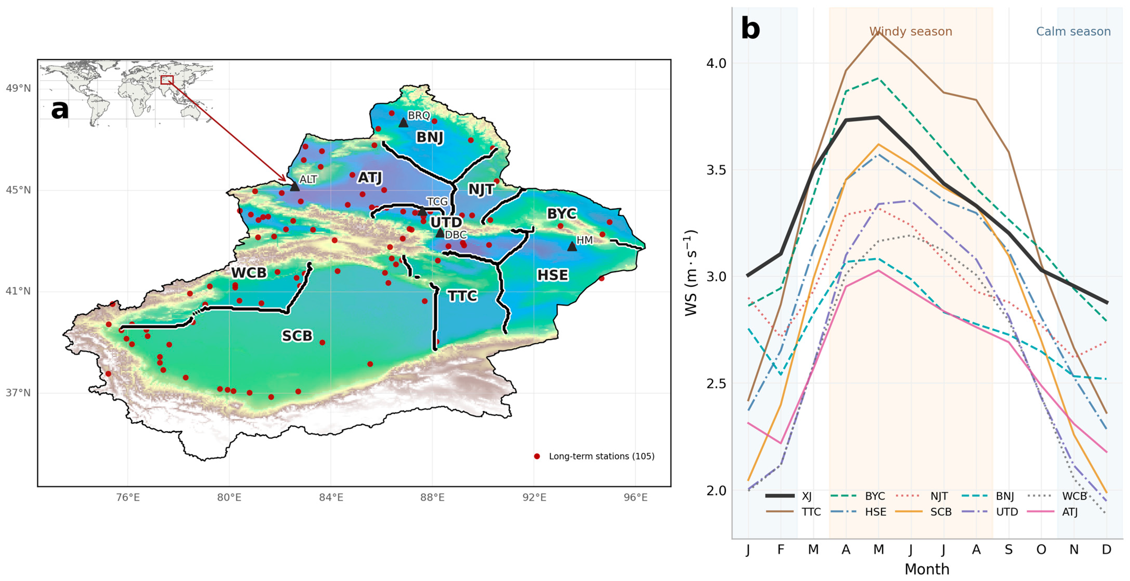
Wind zones were delineated using a two-step terrain-aware clustering framework. In the first step, each grid cell within the Xinjiang developable area was characterized by six normalized features: climatological annual-mean wind speed, elevation, slope, distance to nearest major mountain pass, latitude, and longitude. A KMeans algorithm (k = 24) was then applied to these six-dimensional feature vectors to identify representative seed clusters. In the second step, these seeds were expanded into spatially contiguous sub-regions via a graph-based shortest-path assignment that penalizes transitions across steep slopes, high-elevation barriers, large elevation jumps, and strong wind-climatology discontinuities. Finally, the 24 initial sub-regionss were physically merged into nine refined wind energy assessment zones (Z1–Z9) according to terrain continuity, mountain-pass corridor structure, and known wind-base distribution. As illustrated in Figure 1b, the monthly mean wind speed across Xinjiang exhibits a pronounced and synchronized unimodal pattern, characterized by “high in spring–summer and low in autumn–winter.” Specifically, April to August constitutes the typical windy season, with wind speeds in most sub-regions peaking in May. Driven by intense topographic funneling, the Turpan–Toksun strong wind channel zone (Z1, TTC) and the Barkol–Yiwu core wind energy zone (Z2, BYC) consistently lead the region throughout the year, with the May peak in TTC exceeding 4.0 m/s. Monthly wind speeds in the Southeastern Hami wind corridor (Z3, HSE), Northeastern Junggar transitional zone (Z4, NJT), Southern Xinjiang western–central basin wind belt (Z5, SCB), Burqin–Northern Junggar wind zone (Z6, BNJ), and Urumqi–Tiechanggou–Dabancheng wind corridor (Z7, UTD) fluctuate around the regional average (XJ). A calm season emerges from November to the following February, during which wind speeds drop sharply; notably, winter wind speeds in the western–central intermountain sheltered basin zone (Z8, WCB) and the Alataw Pass–Tacheng–Western Junggar wind corridor (Z9, ATJ) bottom out below 2.5 m/s. These profiles demonstrate the coexistence of high temporal concentration and pronounced spatial heterogeneity in Xinjiang’s wind energy resources.
Wind power zones are delineated based on the 1979–2018 monthly mean wind speed climatology from the WRF dataset, combined with geomorphological units and the distribution of major wind power bases. The climatological mean wind speed for each month is first calculated at each grid point, and the annual mean wind speed, peak month and annual range are then used as primary descriptors or initial regional classification. These preliminary regions are subsequently merged and adjusted to Tianshan geomorphological boundary, the continuity of mountain-pass corridors, and the distribution of major wind power bases to obtain the final nine zones (Z1–Z9). Zone boundaries and 12-month climatology curves are overlaid on Figure 1. Based on this monthly climatology, four wind seasons are defined for subsequent analysis: the windy season (April–August), when peak wind speed and maximum power production occur across all zones; Transition Season I (March), bridging the onset of the high-wind period; Transition Season II (September–October), bridging its decay; and the calm season (November–February), characterized by suppressed wind speeds under stable stratification. For seasonal comparison of capacity factor and equivalent full-load hours (Section 3.2), three aggregate groups are used: high-wind (April–August), transition (March and September–October combined), and low-wind (November–February). Interannual variability of seasonal CF and EFLH is quantified by the standard deviation across the 40 annual values (1979–2018) and displayed as error bars.

2.2. Data Sources

Three categories of data are used in this study:
(1) WRF Dynamical Downscaling Wind Field Data. The East Asian Reanalysis 40-year (EAR40) dataset spanning 1979 to 2018 is a validated spatial proxy. The EAR40 dataset was generated through dynamical downscaling of the global ERA-Interim reanalysis using the Weather Research and Forecasting (WRF, v3.7.1) model and enhanced by a Four-Dimensional Data Assimilation (FDDA) scheme that incorporated surface observations from over 2400 CMA stations to improve accuracy. The model configuration utilized 36 h simulation cycles—discarding the initial 12 h for spin-up—and employed a robust suite of physical parameterizations, including the Thompson microphysics scheme, Dudhia shortwave radiation scheme, RRTM longwave radiation scheme, Yonsei University (YSU) planetary boundary layer scheme, revised MM5 Monin–Obukhov surface layer scheme, Kain–Fritsch cumulus parameterization, and the Jiménez and Dudhia sub-grid topographic wind speed correction (topo_wind = 1) to account for unresolved terrain-induced acceleration and deceleration effects on near-surface winds. Horizontal turbulent mixing was represented using two-dimensional Smagorinsky first-order closure. Furthermore, the Unified Noah land surface model was integrated. The dataset provides the U (zonal) and V (meridional) wind speed components at 10 m height. It has been validated in complex mountain-basin wind energy assessments [23], reanalysis product evaluation across Yangtze River [24], and nationwide wind speed error analysis [25], demonstrating superior near-surface wind speed reproduction over global reanalysis products in complex terrain. The 10 m wind speed is calculated as:
W S 10 = U 2 + V 2
(2) GIMMS NDVI Data. The Global Inventory Modeling and Mapping Studies (GIMMS) NDVI3g dataset [26], derived from AVHRR sensors with a spatial resolution of approximately 8 km and bimonthly temporal resolution (1981–2015), is used to estimate the aerodynamic roughness length ( z 0 ) at each grid point. The z 0 values are derived from NDVI using the empirical exponential relationship [27]:
z 0 = e x p 5.5 + 5.8 N D V I
This formulation yields z 0 values ranging from approximately 0.004 m (bare desert, NDVI ≈ 0.05) to 0.5 m (dense vegetation, NDVI ≈ 0.7), consistent with field observations in semi-arid terrain [27]. This NDVI-based approach provides spatially continuous roughness estimates suitable for regions with heterogeneous and sparse vegetation cover, such as Xinjiang, serving as a key parameter for wind speed height extrapolation (Equation (3)).
(3) Surface Observation Validation Data. Long-term hourly wind speed records from 105 stations (1979–2013), quality-controlled by the Xinjiang Meteorological Information Center, are used to assess climatological bias and temporal correlation of WRF wind speeds across seasons and zones (Section 3.1).

2.3. Wind Speed Extrapolation and Power Output Calculation

The hub-height wind speed is extrapolated from 10 m using the power law [28,29]:
v h = v h 0 h h 0 α
where v h is the wind speed at hub height h = 100 m, which is adopted as the primary analysis level because it is broadly representative of current onshore wind-turbine hub heights; v h 0 is the wind speed at h 0 = 10 m; and α is the wind shear exponent estimated from z 0 via the empirical relation α = 1 / l n h ref / z 0 [28,29], with z 0 obtained from Equation (2).
A representative turbine power curve is configured per IEC 61400 [30]: cut-in speed v in = 3 m/s, rated speed v r = 11 m/s, and cut-out speed v out = 25 m/s. Hourly power output is calculated as [13]:
P v = 0 , v < v in   or   v > v out P r v 3 v in 3 v r 3 v in 3 , v in v < v r P r , v r v v out
where P r is the rated capacity. Wind power density (WPD) at hub height is:
  W P D = 1 2 ρ v 3 ¯
where ρ = 1.225 kg·m−3, and v 3 ¯ is the mean cubed wind speed [5]. The capacity factor (CF) and equivalent full-load hours (EFLH) are:
C F = t = 1 N P t N P r
E F L H = C F × T
where N is the number of hours in the evaluation period, and T is the corresponding total hours (8760 h for a full year, or the seasonal hour count).

2.4. Validation and Trend Analysis

Validation Metrics. WRF-simulated 10 m wind speeds are validated against 105 stations’ observations separately by wind season and zone to reveal terrain- and season-dependent error structures. Three metrics are used [31]:
M E = 1 N t = 1 N v sim , t v obs , t
R M S E = 1 N t = 1 N v sim , t v obs , t 2
R = t = 1 N v sim , t v sim v obs , t v obs t = 1 N v sim , t v sim 2 t = 1 N v obs , t v obs 2
Here, ME quantifies systematic bias, RMSE captures both systematic and random components, and R measures the model’s temporal tracking ability. Domain-average and zone-level metrics are reported to reveal inter-zone cancelation. Based on the combination of |ME| and R, zones are classified into three quality groups: Group 1 (|ME| < 0.5 m·s−1 and R > 0.45)—suitable for direct use; Group 2 (|ME| < 0.5 m·s−1 and 0.35 ≤ R ≤ 0.45)—usable with caution; and Group 3 (|ME| ≥ 0.5 m·s−1 or R < 0.35)—requiring zone-specific bias correction before application (Section 3.1).
Long-term Trends. Linear trends of annual WS and WPD at 100 m are estimated using Sen’s slope estimator, with significance tested by the Mann–Kendall method ( p < 0.05). Trend coefficients are expressed per decade (m·s−1·decade−1; W·m−2·decade−1) and mapped spatially.
Interannual Anomalies. WS and WPD anomalies are computed for the full domain and each zone by subtracting the 1979–2018 climatological mean and presented as heatmaps to identify decadal phases and zone-level trend divergence.
Decadal Decomposition. The 40-year record is divided into four periods (1979–1988, 1989–1998, 1999–2008, and 2009–2018). Decadal-mean WS and WPD are computed per zone and further decomposed by high-wind versus calm seasons to determine which season dominates decadal variability.

2.5. Diurnal Cycle Analysis

Hourly CF values at 100 m are averaged across all days within each decadal period to construct composite diurnal profiles for the full domain and each zone, stratified by high-wind and calm seasons. All times are in local standard time (LST = UTC + 6). Diurnal profiles for all nine zones are provided in Figure A1.
For each hour h (0–23 LST), the departure from the daily mean is:
Δ C F h = C F h ¯ 1 24 h = 0 23 C F h ¯
This metric isolates diurnal amplitude and phase from the absolute CF level. Phase stability is assessed by comparing the hour of peak CF and the diurnal amplitude among the four decadal periods.

2.6. Extreme Wind Power Ramp Event Identification

Extreme ramp events are defined as hours during which the absolute hourly change in capacity factor exceeds a prescribed threshold:
Δ C F t = C F t C F t 1 > δ
where δ = 0.10 (i.e., a 10 percentage-point hourly CF change), applied uniformly across all zones. This threshold corresponds to a power swing of 10% of rated capacity within one hour, a level at which grid frequency regulation reserves are typically activated [17]. Three characteristics are computed annually per zone and season:
Event Frequency: The number of ramp events exceeding the threshold per year.
Mean Ramp Rate:
R R ¯ = 1 n i = 1 n Δ C F i Δ t × 100 % h 1
where n is the annual event count and Δ t = 1 h.
Maximum Shock Intensity:
S I max = m a x i = 1 , , n Δ C F i Δ t × 100 % h 1
Annual anomalies of all three metrics are presented as heatmaps, stratified by zone and season, to identify temporal clustering of ramp risk and to assess whether ramp trends are coupled with or decoupled from mean wind speed trends (Section 3.3).

3. Results

3.1. Accuracy Verification of WRF-Simulated Wind Field Data

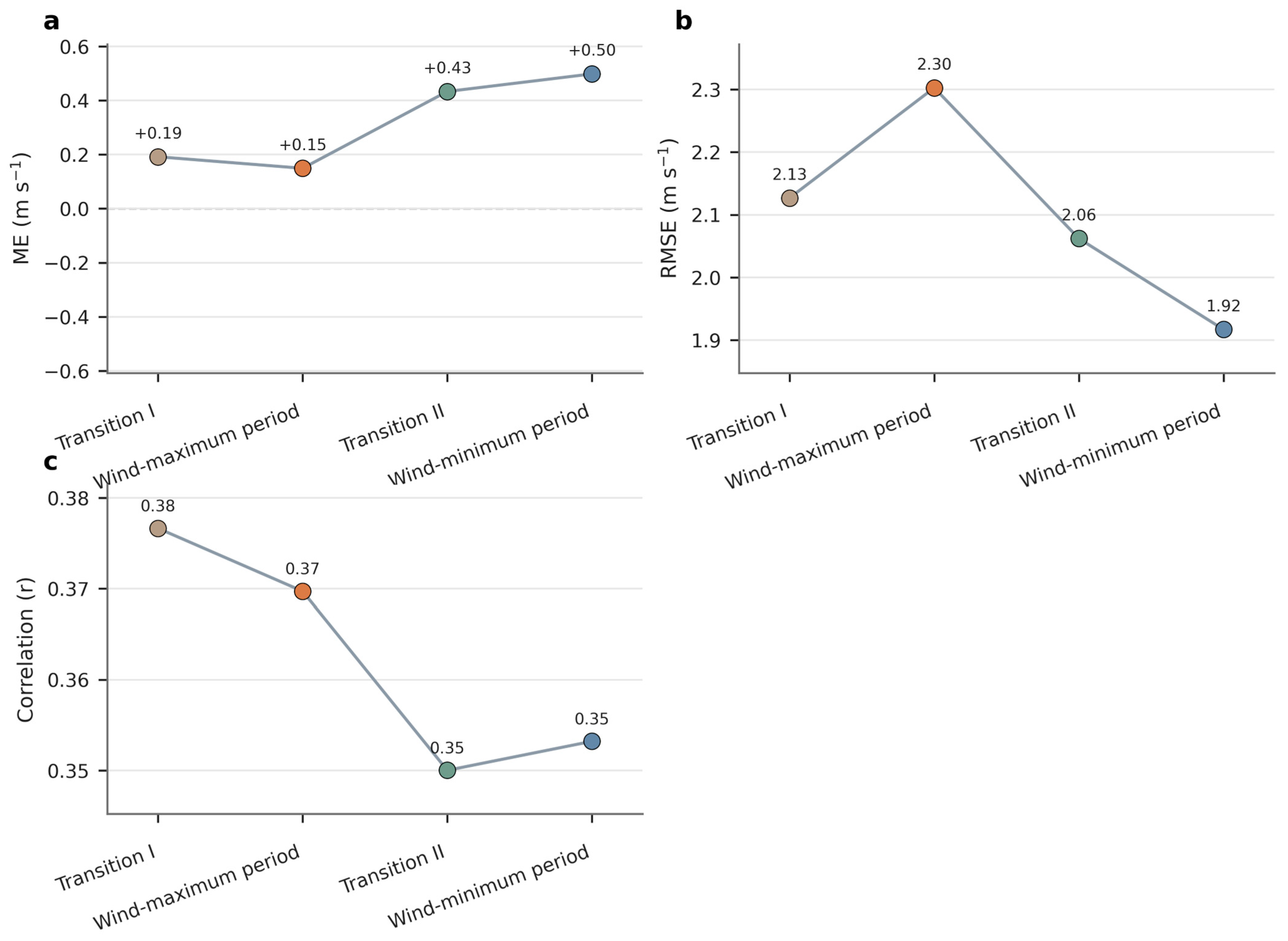
Figure 2 presents the mean error (ME), root mean square error (RMSE), and correlation coefficient (R) of WRF-simulated 10 m wind speed against observations for the entire Xinjiang domain, stratified by wind season. ME is positive in all four seasons, indicating a systematic overestimation of near-surface wind speed. The windy season (April–August) has the smallest ME at +0.15 m·s−1. Transition Season I yields +0.19 m·s−1, Transition Season II +0.43 m·s−1, and the calm season (November–February) has the largest at +0.50 m·s−1. The increase from the high-wind season to the calm season is 0.35 m·s−1. This seasonal amplification of positive bias is attributable to insufficient momentum dissipation under stable boundary layer conditions in winter, compounded by possible low bias in observations due to anemometer starting thresholds at low wind speeds. RMSE follows an opposite seasonal pattern: it peaks at 2.30 m·s−1 in the windy season, decreases to 2.13 m·s−1 in Transition I, 2.06 m·s−1 in Transition II, and reaches a minimum of 1.92 m·s−1 in the calm season. The windy season RMSE is driven by large background wind magnitudes and frequent gusts that amplify the random error component instead of causing a systematic departure. In the calm season, low RMSE combined with high ME confirms that the error structure is dominated by a steady positive offset with a small random component. R ranges from 0.35 to 0.38 across seasons. Transition I is highest (0.38), followed by the windy season (0.37); Transition II and the calm season are 0.35 each. The cross-season range is only 0.03, indicating that the model’s ability to track temporal wind variability driven by synoptic-scale circulation remains stable regardless of season. The overall R below 0.40 reflects the influence of local thermal circulations and terrain-induced turbulence at the hourly scale, which WRF’s horizontal resolution cannot fully resolve. It may also reflect representativeness mismatch between point observations and model grid cells, as well as differences in station data quality and maintenance conditions. For wind energy assessment, the low ME in the windy season supports reliable estimation of bulk power output. For low-output risk assessment, the persistent positive bias in the calm season may lead to underestimation of calm-period duration, a consideration for future operational applications.
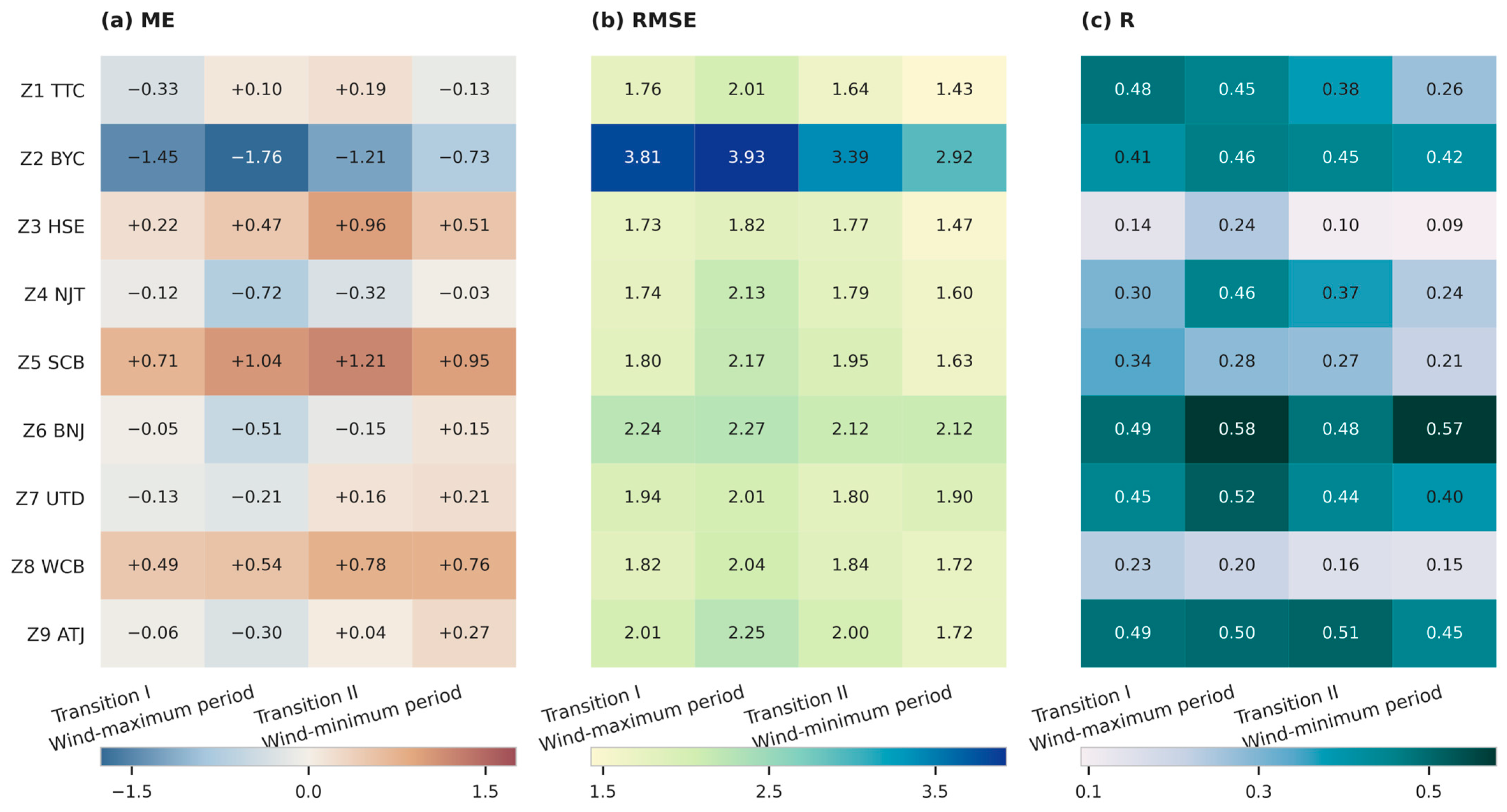
Figure 3 displays ME, RMSE, and R for zones Z1–Z9 in four wind seasons as heatmaps. The regional decomposition reveals strong inter-zone cancelation masked by the domain-average statistics. ME direction diverges fundamentally among zones. Z2 (BYC) shows negative bias in all seasons: −1.45 m·s−1 in Transition I, −1.76 m·s−1 in the windy season, −1.21 m·s−1 in Transition II, and −0.73 m·s−1 in the calm season. The model severely underestimates actual wind speed in this zone, with the largest deficit in the windy season. This is consistent with inadequate resolution of gap-flow acceleration in the complex valley terrain. Z5 (SCB) exhibits persistent positive bias across all seasons: +0.71, +1.04, +1.21, and +0.95 m·s−1. Z8 (WCB) is also consistently overestimated (+0.49 to +0.78 m·s−1). Z3 (HSE) shows positive bias peaking at +0.96 m·s−1 in Transition II. Z1 (TTC) has the best-controlled ME, fluctuating within −0.33 to +0.19 m·s−1, with all absolute values below 0.35 m·s−1. Most northern zones (Z4, Z6, Z7, Z9) exhibit a seasonal sign reversal: slight underestimation in the windy season and slight overestimation in the calm season. For RMSE, Z2 is far above other zones in all seasons: 3.81, 3.93, 3.39, and 2.92 m·s−1. Other zones fall within 1.43–2.27 m·s−1, with Z1 the lowest (1.43–2.01 m·s−1). R exhibits a clear spatial gradient. Z6 (BNJ) ranks the highest: 0.49, 0.58, 0.48, and 0.57. Z9 (ATJ) follows: 0.49, 0.50, 0.51, and 0.45. Z7 (UTD) yields 0.45, 0.52, 0.44, and 0.40. Z3 (HSE) is the lowest with 0.09, 0.24, 0.15, and 0.12, indicating the poorest temporal tracking in this zone. Z2, despite large ME and RMSE, maintains R at 0.41–0.46, meaning the model captures temporal variability but with a systematic offset. Based on these metrics, the nine zones fall into three groups: Group 1 (Z6, Z9, Z7)—small ME and high R, suitable for direct use; Group 2 (Z1, Z4)—small ME but moderate R; and Group 3 (Z2, Z3, Z5, Z8)—large systematic bias or low R, requiring zone-specific bias correction before application.
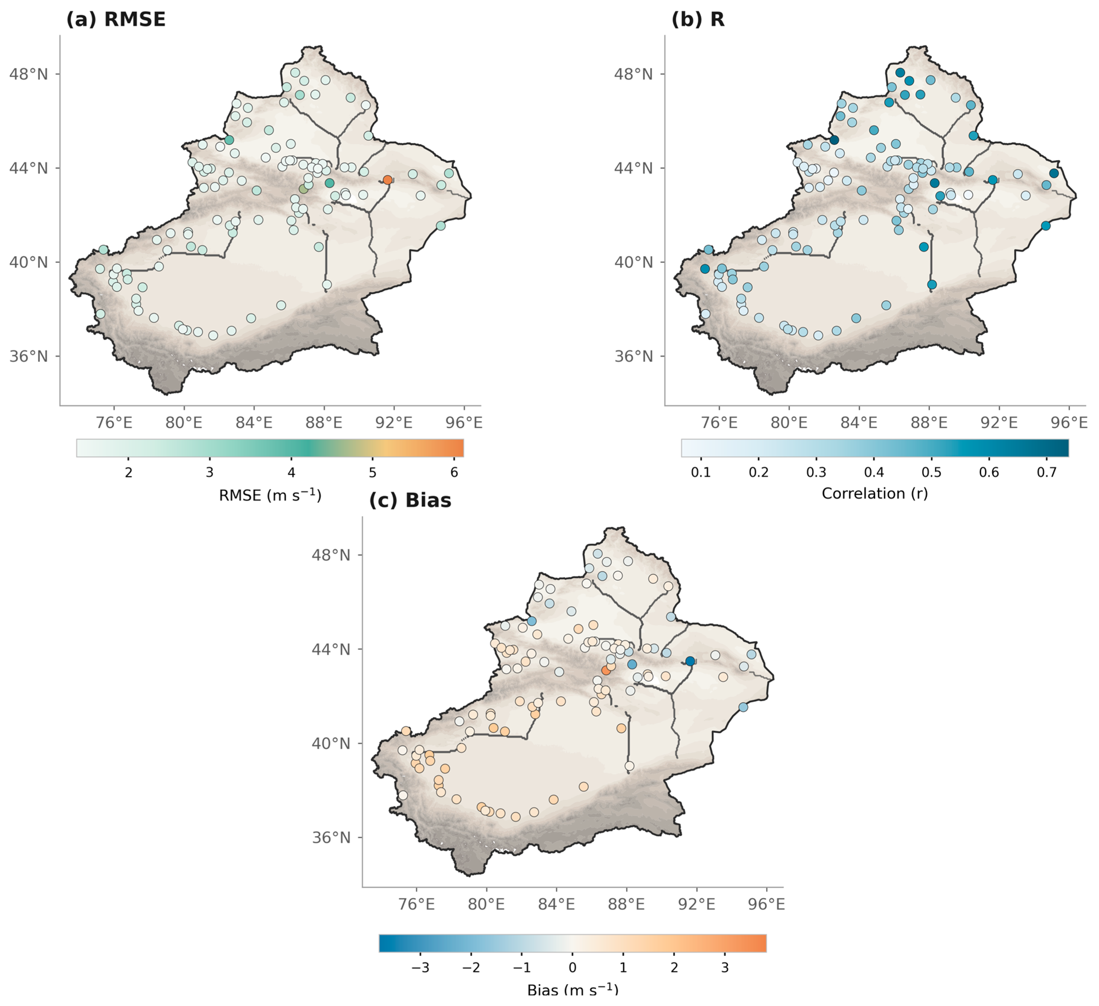
Figure 4 presents three statistical metrics—root mean square error (RMSE), correlation coefficient (R), and bias—computed from WRF simulations against four daily (00, 06, 12, 18 UTC) observations at 105 meteorological stations across Xinjiang during 1979–2013. Figure 4a shows that station-level RMSE values range from 2.0 to 6.0 m/s with distinct regional patterns. Stations within and along the margins of the Tarim Basin exhibit the lowest RMSE, predominantly between 2.0 and 2.5 m/s. Stations across the Junggar Basin and its periphery display moderate values of 2.5–3.5 m/s. In contrast, stations near the Tianshan Mountains and in Eastern Xinjiang show markedly elevated RMSE, with several sites exceeding 4.0 m/s and isolated stations reaching 5.0–6.0 m/s. Figure 4b reveals a pronounced north–high, south–low spatial pattern in correlation coefficients. Northern Xinjiang stations, particularly in the Altay region and along the Northern Junggar Basin margin, achieve R values above 0.5, with selected sites reaching 0.6–0.7. Stations along the Tianshan range cluster between 0.3 and 0.5. Southern Xinjiang stations within the Tarim Basin show the weakest temporal agreement, with R values largely confined to 0.1–0.3. Figure 4c indicates that bias values across most stations fall between −3.0 and +3.0 m/s. The Tarim Basin and surrounding stations exhibit widespread positive bias of +0.5 to +2.0 m/s, indicating systematic overestimation. Junggar Basin stations show mild positive bias near 0 to +1.0 m/s. Notably, several stations in terrain-complex junctions near the Tianshan Mountains and Eastern Xinjiang display negative bias extremes of −2.0 to −3.0 m/s, suggesting localized underestimation in regions characterized by channeling effects. Overall, WRF performance is strongly terrain-dependent: the Tarim Basin features low RMSE but weak temporal correlation and systematic overestimation; Northern Xinjiang exhibits the highest correlation (R > 0.5) with slight positive bias; and mountainous and eastern regions show elevated absolute errors (RMSE > 5.0 m/s locally) with localized negative bias below −2.0 m/s.

3.2. Spatial Distribution and Seasonal Climatology of Wind Energy Resources

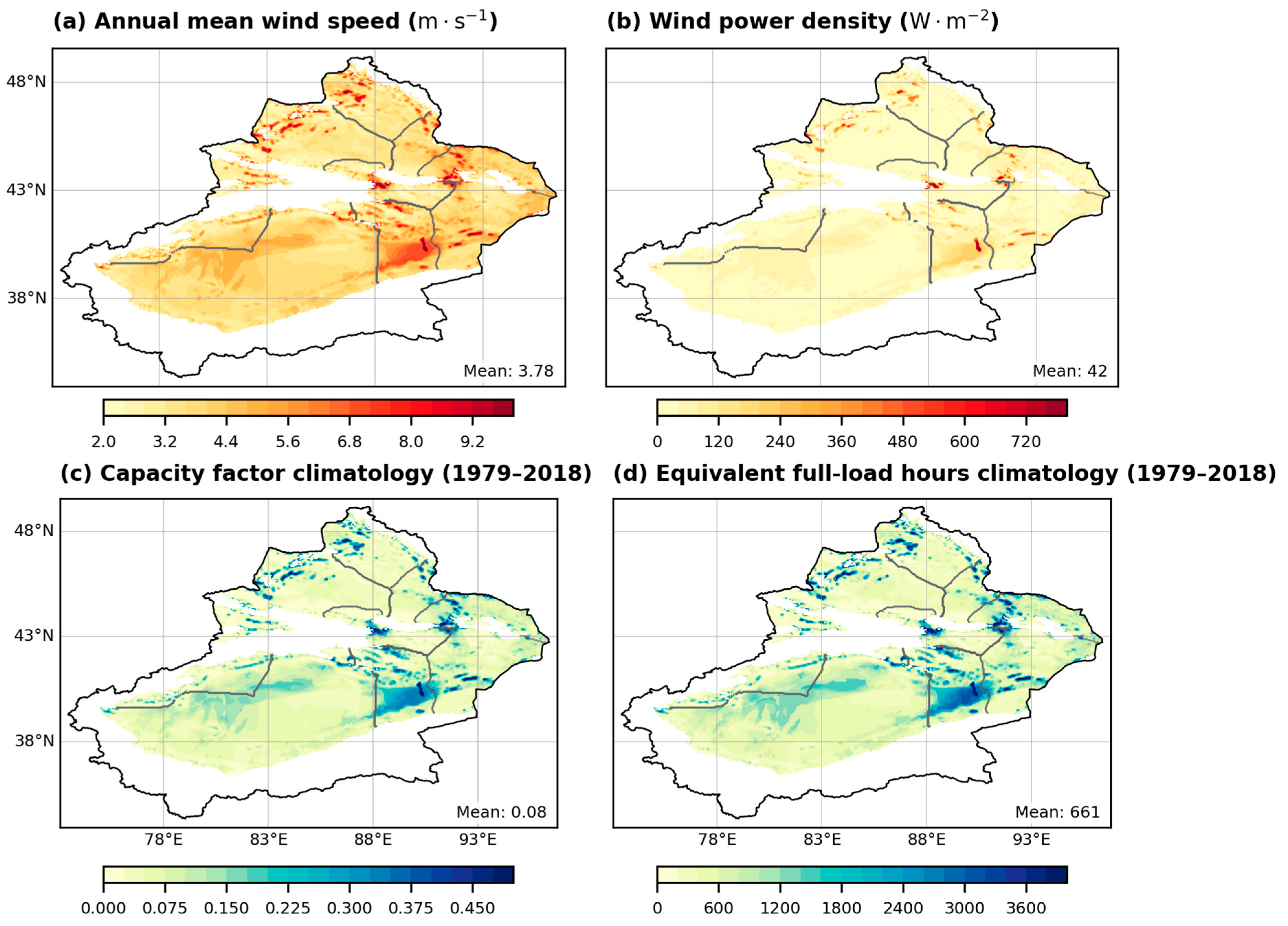
Figure 5 maps the 1979–2018 climatological mean wind speed (WS, Figure 5a), wind power density (WPD, Figure 5b), capacity factor (CF, Figure 5c), and equivalent full-load hours (EFLH, Figure 5d) at 100 m height across Xinjiang. All four fields share a coherent spatial structure dominated by terrain-controlled channeling, featuring narrow high-value corridors along mountain passes and gorges surrounded by extensive low-value basins. As shown in Figure 5a, domain-mean WS is 3.78 m·s−1, with prominent maxima in Z1 (TTC) exceeding 6.0 m·s−1 and locally reaching 7.0–8.5 m·s−1, followed by Z7 (UTD) at 5.5–7.0 m·s−1, Z9 (ATJ) at 5.0–6.5 m·s−1, and Z2 (BYC) at 5.0–6.0 m·s−1, whereas the interior Tarim Basin (Z5) is broadly below 3.0 m·s−1 and the Central Junggar Basin remains at 3.0–3.5 m·s−1. Due to the cubic relationship between wind speed and power, the WPD field (Figure 5b) exhibits far more extreme spatial contrasts: the domain mean is only 42 W·m−2, yet the Z1 core exceeds 480 W·m−2 with local peaks of 600–800 W·m−2, Z7 ranges 240–480 W·m−2, Z9 180–360 W·m−2, and Z2 120–240 W·m−2, while basin interiors fall below 60 W·m−2 and Z5 below 30 W·m−2 over large areas. The CF distribution (Figure 5c) mirrors this pattern, with a domain mean of 0.08; Z1 core values reach 0.35–0.45, Z7 0.20–0.35, Z9 0.15–0.25, and Z2 0.12–0.20, whereas most basin areas remain below 0.05. Correspondingly, Figure 5d shows that domain-mean EFLH is 661 h, with Z1 attaining 3000–3900 h, Z7 1800–3000 h, Z9 1300–2200 h, and Z2 1000–1800 h, while basin interiors are below 450 h and Z5 broadly below 250 h. Applying the industry benchmark of EFLH > 2000 h for economic viability, only the cores of Z1, Z7, and parts of Z9 qualify, indicating that exploitable wind energy resources are highly concentrated in a few terrain-favored corridors where multiple wind farms are likely to experience synchronized output fluctuations.
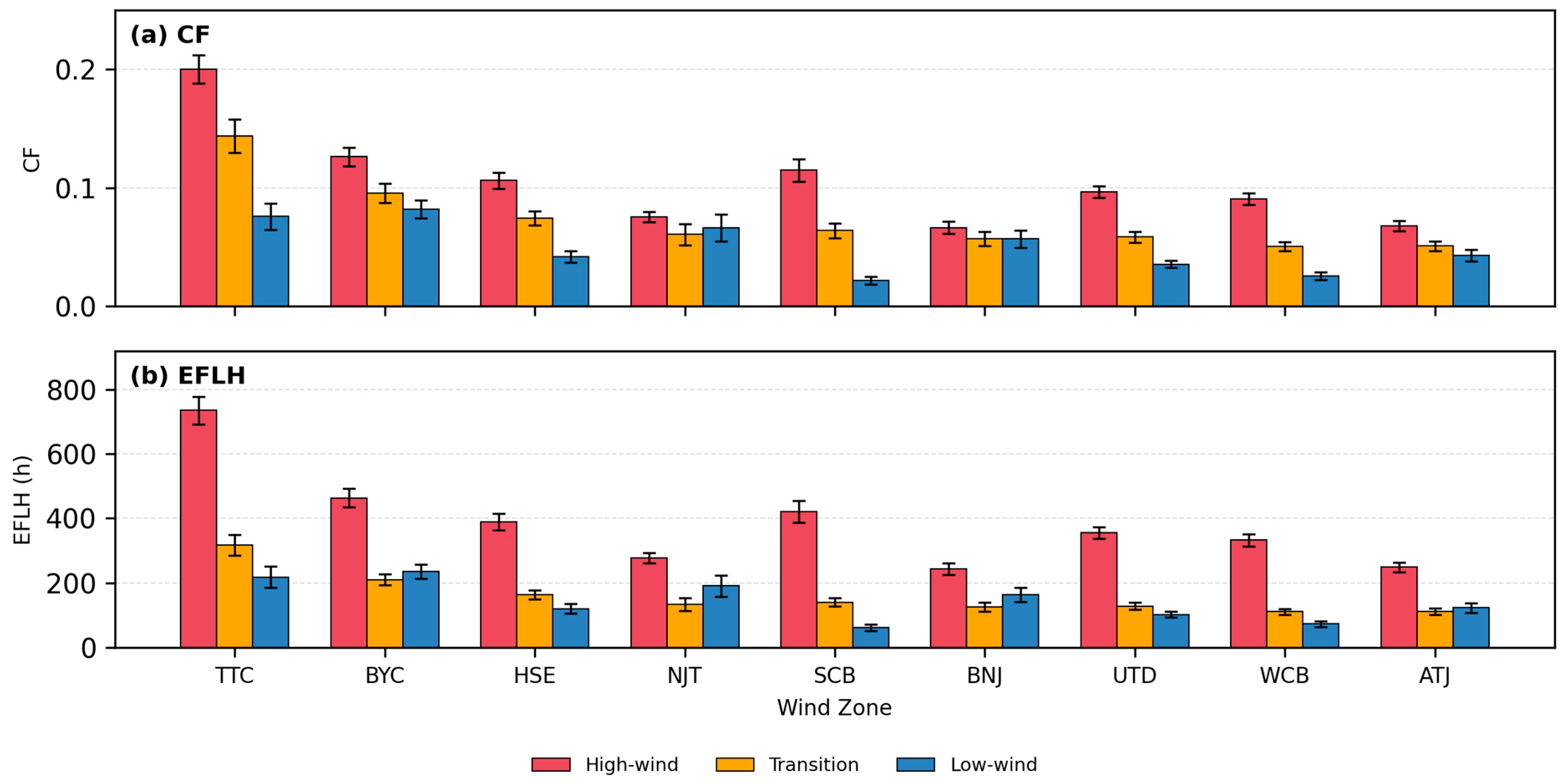
Figure 6 compares CF (Figure 6a) and EFLH (Figure 6b) across nine zones for three seasonal groups—high-wind (April–August), transition (March and September–October), and low-wind (November–February)—with error bars denoting interannual standard deviation. All zones peak in the high-wind season, but the degree of seasonal imbalance differs substantially. In Figure 6a, Z1 (TTC) has the highest high-wind CF at ~0.198, followed by transition ~0.143 and low-wind ~0.078, yielding a high-to-low ratio of ~2.5 that represents the largest seasonal amplitude among all zones. Z2 (BYC) shows high-wind CF ~0.127, transition ~0.098, and low-wind ~0.083, with a ratio of only ~1.5, indicating relatively mild seasonal contrast and sustained winter output. Z5 (SCB) exhibits the most extreme seasonal asymmetry, with high-wind CF ~0.115 but low-wind only ~0.022, yielding a ratio of 5.2 with winter output near zero. Z6 (BNJ) has the most uniform seasonal distribution, with CF tightly clustered at 0.055–0.065 across all three seasons, though the absolute level is low. Error bars in Figure 6a are longest for Z1 in the high-wind season (~±0.04), indicating large interannual variability, whereas Z6 error bars are short (~±0.01) in all seasons and Z5 low-wind error bars are minimal (~±0.005), confirming that winter low output is nearly invariant year to year. Correspondingly, Figure 6b shows that Z1 high-wind EFLH yields ~730 h, transition ~315 h, and low-wind ~225 h, totaling ~1270 h with the high-wind season contributing ~57%. Z2 high-wind reaches ~465 h, transition ~215 h, and low-wind ~240 h, where the low-wind value slightly exceeds transition. Z5 high-wind attains ~420 h but low-wind only ~65 h, with the high-wind share reaching ~69%, implying the highest cross-seasonal storage requirement. Z6 distributes more evenly (240/120/170 h), with the high-wind share below 50%. Z4 (NJT) low-wind EFLH (~180 h) exceeds its transition value (~150 h), similar to Z2, indicating that Northeastern Junggar is not entirely calm in winter. These results demonstrate that annual mean values alone are insufficient for evaluating development potential; the seasonal concentration ratio directly determines storage sizing and dispatch strategy.

3.3. Long-Term Evolution and Decadal Trends of Wind Energy Resources

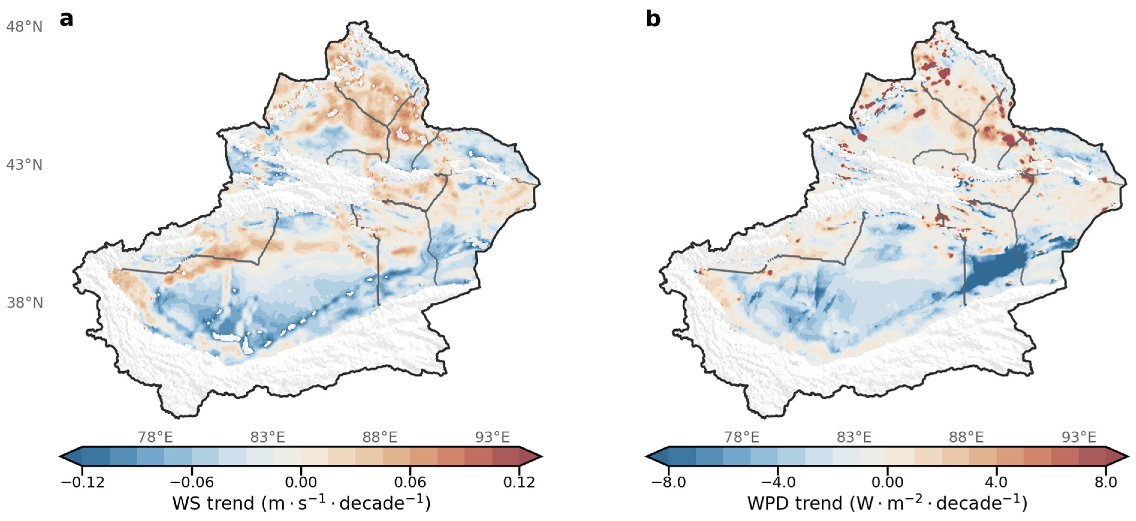
Figure 7 maps the linear trend coefficients of WS (Figure 7a) and WPD (Figure 7b) at 100 m height during 1979–2018, with color scales spanning −0.12 to +0.12 m·s−1·decade−1 for WS and −8 to +8 W·m−2·decade−1 for WPD. Positive and negative trend areas are interspersed across both panels, forming a coherent pattern of “northern local enhancement, southern basin weakening, and internal differentiation within pass corridors.” In Figure 7a, Northern Xinjiang emerges as the primary area of positive WS trends, as Z6 (BNJ) and the northern margin of Z4 (NJT) show broad areas at +0.03 to +0.09 m·s−1·decade−1, with isolated grid points near the upper bound of +0.12 m·s−1·decade−1, while western Z9 (ATJ) near Alataw Pass also contains scattered positive patches. Southern Xinjiang is dominated by negative trends, with Z5 (SCB) in Western and Central Tarim Basin showing continuous negative values of −0.03 to −0.09 m·s−1·decade−1 and the southwestern corner approaching −0.12 m·s−1·decade−1; the southern margin of Z3 (HSE) also contains a negative patch at approximately −0.06 m·s−1·decade−1. Z1 (TTC) displays a mosaic of positive and negative values in Figure 7a, as the core corridor is slightly positive (~+0.03 m·s−1·decade−1), while the southern and eastern flanks are negative, suggesting that sub-grid topographic heterogeneity within the same pass may modulate the local response to large-scale climate forcing. Z7 (UTD) shows near-zero or weakly positive trends, and the Tianshan ridge zone (~42–43° N) remains near zero throughout. The WPD trend field (Figure 7b) mirrors the WS spatial pattern but with amplified contrast due to the cubic relationship between wind speed and power. Z6 contains multiple grid points at +4 to +8 W·m−2·decade−1, with some exceeding the color scale limit, as even a modest WS increase of +0.06 m·s−1·decade−1 produces substantial WPD gains in areas with high baseline wind speed. Z5’s southwestern WPD trends reach −4 to −8 W·m−2·decade−1 in Figure 7b. The area of positive WPD trends is smaller than the negative area, yet positive trends are spatially co-located with existing operational wind bases (Burqin, Alataw Pass), indicating that the resource endowment of northern trunk wind bases has not deteriorated over the past 40 years.
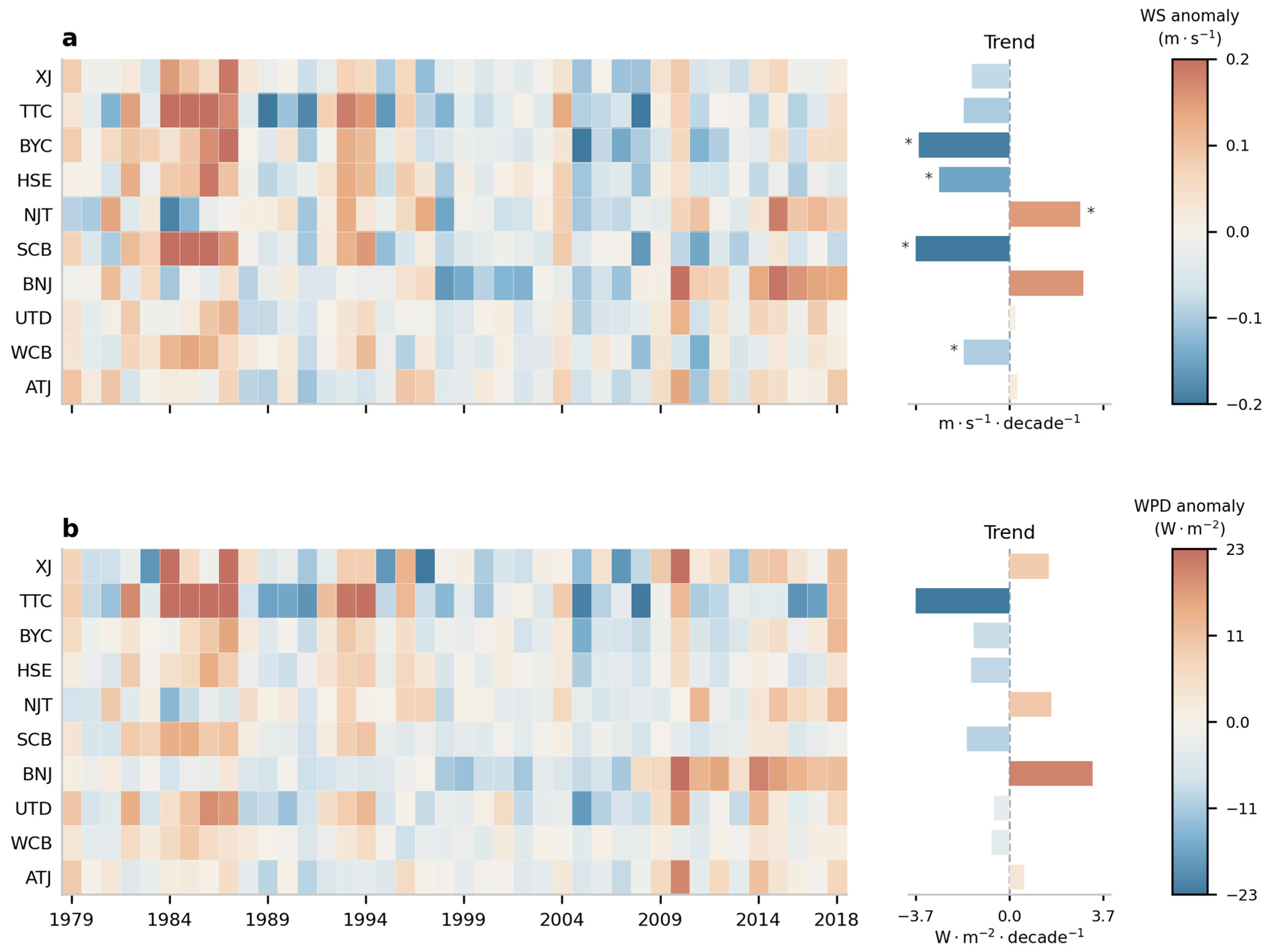
Figure 8 presents WS (Figure 8a) and WPD (Figure 8b) anomaly heatmaps for the full domain (XJ) and each zone during 1979–2018, with bar charts on the right side showing linear trend magnitudes and asterisks denoting significance at p < 0.05 via the Mann–Kendall test. In Figure 8a, the WS anomaly color scale spans approximately −0.20 to +0.20 m·s−1, and three domain-wide decadal phases are identifiable: 1984–1988 as a concentrated positive-anomaly phase, with multiple zones recording +0.10 to +0.15 m·s−1; 1996–2003 as a transitional period, with alternating signs; and 1999–2008 as a concentrated negative-anomaly phase, with 2004–2008 as the strongest segment. The XJ trend bar is weakly negative without an asterisk, indicating no significant domain-wide trend due to inter-zone cancelation. Zone-level divergence in Figure 8a consolidates after 2006, separating into a declining group and an increasing group. Among the declining zones, Z2 (BYC) is covered by nearly continuous blue after 2004 with a significant negative trend; Z3 (HSE) shows positive anomalies in 1985–1988 and increasing negative anomalies after 2005, also with a significant negative trend; Z5 (SCB) has strong positive anomalies in 1984–1988 (+0.10 to +0.18 m·s−1) and persistent negative anomalies in 2005–2018, with a significant negative trend; and Z8 (WCB) shows a significant negative trend smaller in magnitude than Z2 or Z5. Among the increasing zones, Z4 (NJT) shows weak negative anomalies in 1979–1995 turning to continuous positive anomalies in 2010–2018 (+0.05 to +0.12 m·s−1), with a significant positive trend; and Z6 (BNJ) shows densifying positive anomalies after 2006 reaching +0.10 to +0.18 m·s−1 in 2012–2016, recording the strongest significant positive signal among all zones. Z1 (TTC) records +0.18 m·s−1 in 1984, while negative anomalies dominate 1999–2008, with −0.15 m·s−1 in 2005, before weak positive anomalies return in 2009–2014; its trend is negative without significance. The WPD anomaly field (Figure 8b) spans approximately −23 to +23 W·m−2, with spatial and temporal patterns mirroring Figure 8a but with amplified absolute anomalies in high-wind zones; Z6 records WPD positive anomalies of +10 to +20 W·m−2 in 2012–2016, whereas Z2 records −15 to −23 W·m−2 in 2004–2010, and significance markers match those in Figure 8a exactly. The positive trends in Z4 and Z6 are driven primarily by sustained post-2006 positive anomalies rather than uniform 40-year increases, and their persistence requires verification with longer records.
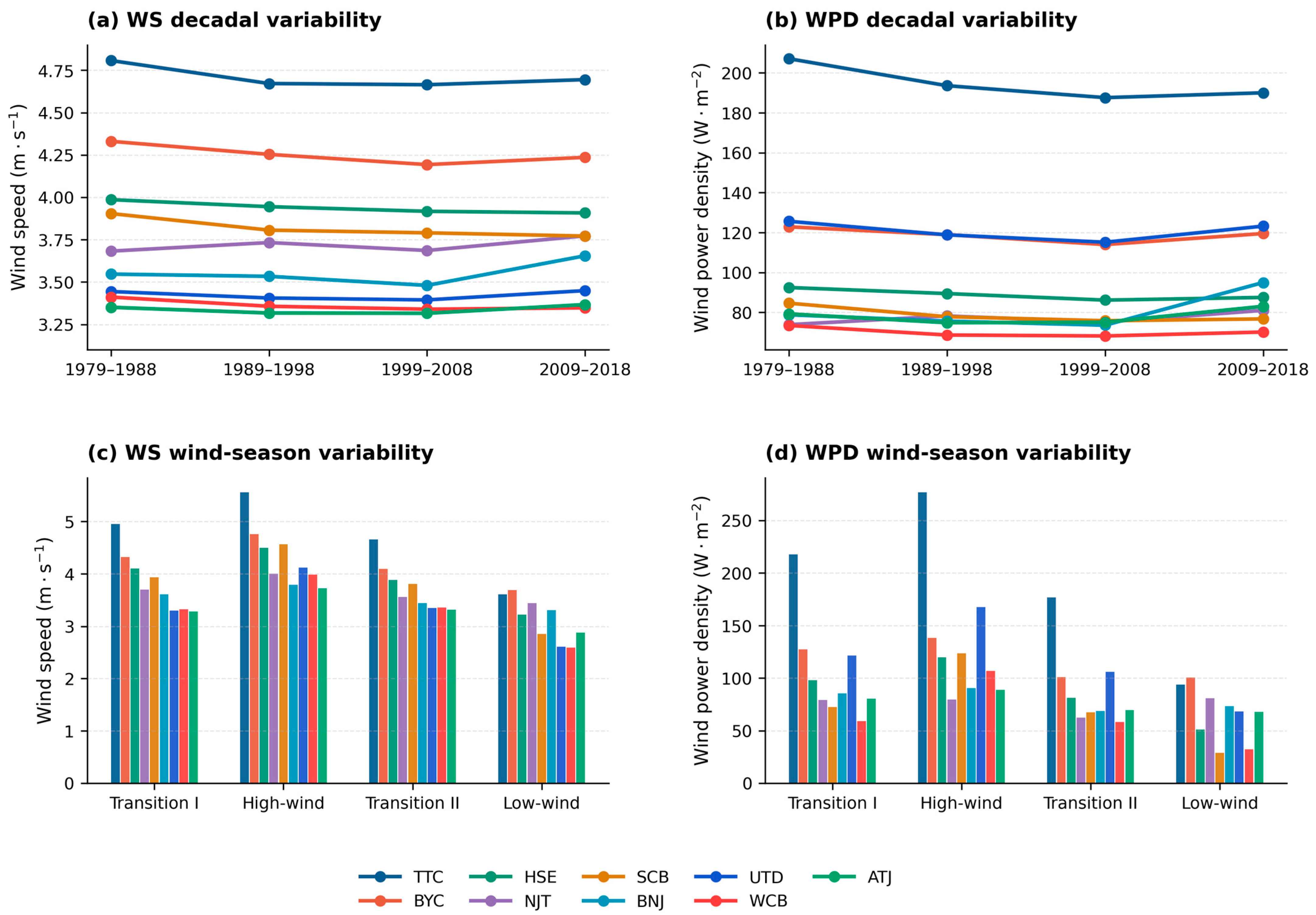
Figure 9 displays decadal-mean WS (Figure 9a) and WPD (Figure 9b) for four periods (1979–1988, 1989–1998, 1999–2008, and 2009–2018), along with their seasonal decomposition (Figure 9c,d). In Figure 9a, Z1 (TTC) maintains the highest WS throughout, 4.81 m·s−1 in the first decade, declining to 4.66 m·s−1 in the third (trough), and then recovering to 4.70 m·s−1 in the fourth, forming a U-shaped trajectory with a 40-year range of 0.15 m·s−1. Z2 (BYC) is the second highest, stepping down from 4.34 to 4.19 m·s−1 before a slight recovery to 4.25 m·s−1. Z7 (UTD) drops from 3.89 to 3.76 m·s−1 and recovers to 3.89 m·s−1, forming a V-shape. Z6 (BNJ) remains near 3.44–3.48 m·s−1 for three decades and rises to 3.55 m·s−1 in the fourth, representing the clearest late-period increase. Z5, Z8, and Z9 stay within 3.3–3.5 m·s−1 with variations below 0.10 m·s−1. In Figure 9b, Z1 WPD declines from 207 to 186 W·m−2 and stabilizes at 190 W·m−2 (range 21 W·m−2), Z7 drops from ~120 to ~110 W·m−2 and recovers to ~125 W·m−2, and Z6 rises from ~74 to ~95 W·m−2 in the fourth decade (increase ~21 W·m−2), while other zones range 70–95 W·m−2 with decadal variations of 10–15 W·m−2.
Figure 9c,d decompose these decadal changes by wind season, revealing that decadal variability is almost entirely driven by the high-wind season. In Figure 9c, high-wind-season WS reaches ~5.50 m·s−1 for Z1, ~4.80 m·s−1 for Z2, and ~4.10 m·s−1 for Z7, whereas in the low-wind season WS drops to 2.6–3.7 m·s−1 across all zones. The corresponding WPD decomposition in Figure 9d shows Z1 high-wind-season WPD at ~275 W·m−2 with a four-decade range of ~30 W·m−2, Z2 at ~140 W·m−2, and Z7 at ~175 W·m−2, while low-wind-season WPD falls below 100 W·m−2 for all zones with Z1 varying by only ~10 W·m−2 across four decades such that the curves nearly overlap. These results indicate that climate variability acts on near-surface wind energy primarily through the high-wind season, manifested as peak-value modulation, whereas the low-wind season, governed by stable stratification, responds minimally to decadal climate signals. Long-term resource assessments should therefore prioritize calibration of variance in the high-wind season.

3.4. Diurnal Variations in Wind Capacity Factors and Peak-Shaving Demands

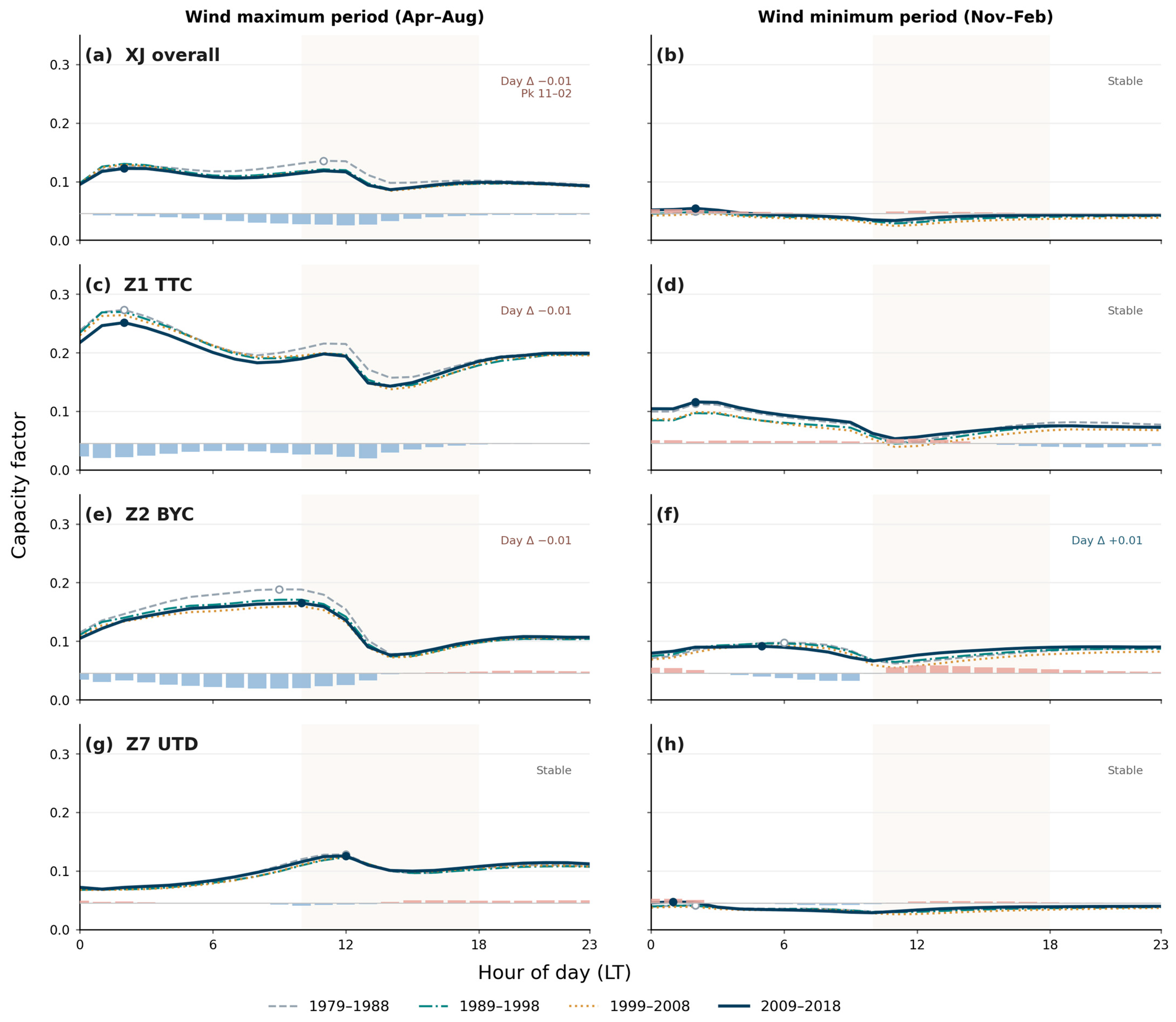
Figure 10 presents hourly CF diurnal profiles for the full domain (XJ) and three representative zones (Z1, TTC; Z2, BYC; Z7, UTD) in the high-wind and low-wind seasons, with four curves corresponding to four decadal periods and bottom bars showing hourly ΔCF departures from the daily mean. In Figure 10a (XJ; high-wind season), CF exhibits a weak bimodal structure: a first peak of ~0.13 at 01–02 LST, a decrease to ~0.11–0.12 at 06–08 LST, a second peak of ~0.12–0.13 at 10–11 LST, and a daily minimum of ~0.09–0.10 at 13–15 LST followed by an evening recovery to ~0.10 by 23 LST, with the annotated peak shift from 11 LST in earlier decades to 02 LST in recent decades corresponding to a CF magnitude change in only ~0.01. In Figure 10b (XJ; low-wind season), CF stays within 0.04–0.055 throughout the day with diurnal amplitude below 0.02, and the four decadal curves nearly overlap, annotated as “Stable.”
Figure 10c (Z1, TTC; high-wind season) shows the largest diurnal amplitude among all panels. CF peaks at 00–02 LST at 0.25–0.27, decreases to ~0.22 by 06 LST and ~0.20 by 10 LST, displays a secondary shoulder at ~12 LST (0.17–0.20, more pronounced in earlier decades), drops rapidly to the daily minimum of 0.14–0.16 at 13–15 LST, and recovers to ~0.20 by 20 LST, yielding a diurnal amplitude of 0.11. Earlier decades are systematically higher by 0.02–0.04, and the day ΔCF is −0.01. The nocturnal peak output is likely related to nocturnal boundary layer processes such as low-level jet formation or drainage flows, although detailed mechanism analysis is beyond the scope of this study. In Figure 10d (Z1; low-wind season), CF ranges 0.05–0.11 with a peak at 00–03 LST (~0.08–0.11) and a trough at 10–12 LST (~0.05–0.06); amplitude is smaller and decadal differences are minimal.
Figure 10e (Z2, BYC; high-wind season) shows CF rising from ~0.09–0.11 at 00 LST to a peak of ~0.17–0.19 at 10–11 LST, dropping rapidly to ~0.09–0.11 at 12–14 LST, and recovering to ~0.10 by 18 LST. In Figure 10f (Z2; low-wind season), CF ranges 0.06–0.10 with a slight peak at 05–06 LST and a trough at ~11 LST (~0.06), with day ΔCF of +0.01.
Figure 10g (Z7, UTD; high-wind season) displays a distinct midday-peak profile differing from Z1 and Z2, where CF is ~0.06–0.07 at 00 LST, rises progressively, peaks at ~0.12–0.13 at 12–13 LST, remains at 0.10–0.11 through 14–16 LST, and decreases slowly to ~0.09 by evening, with four decadal curves tightly overlapping and annotated “Stable.” In Figure 10h (Z7; low-wind season), CF is 0.03–0.05 with negligible diurnal variation. Bottom ΔCF bars across all panels confirm that Z1 and Z2 high-wind diurnal amplitudes are largest (~±0.04–0.05), Z7 is moderate (~±0.02), and all zones in the low-wind season are within ±0.01. Over 40 years, the phase structure of diurnal CF curves has not changed materially, with peak-time decadal shifts confined to −0.01 to +0.01 h. The nocturnal peak at Z1 and Z2 coincides with the photovoltaic off-period, while the midday peak at Z7 can stack with solar output, offering distinct grid-integration complementarity options (see also Figure A1).
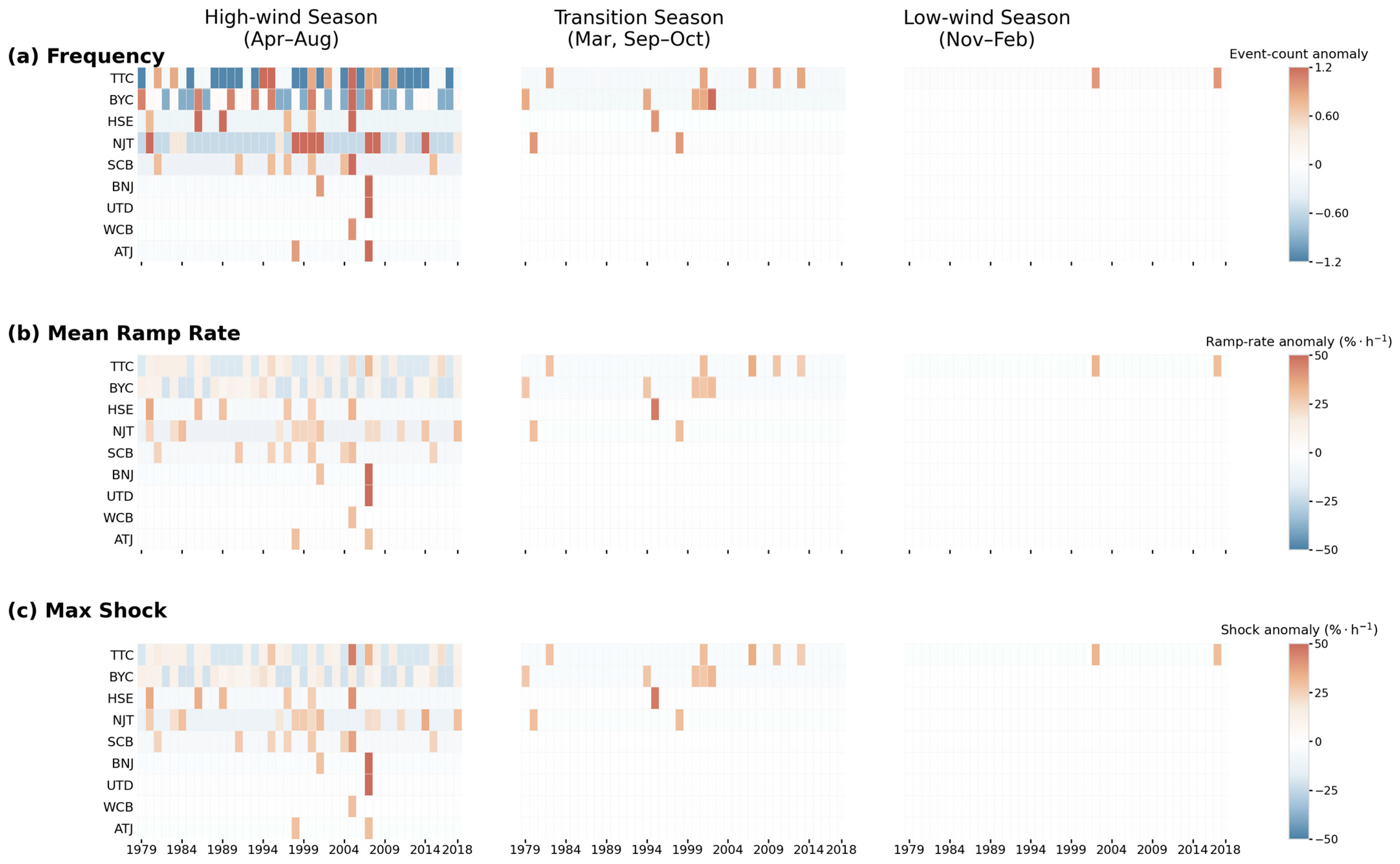
Figure 11 presents heatmaps of annual anomalies in extreme wind power ramp event frequency (Figure 11a), mean ramp rate (Figure 11b), and maximum shock intensity (Figure 11c) for nine zones across three seasonal groups, with color scales spanning −1.2 to +1.2 events for frequency and −50 to +50%·h−1 for ramp rate and shock intensity. In Figure 11a, color-filled cells are almost entirely confined to the high-wind season, transition seasons contain sparse entries, and the low-wind season is blank throughout, confirming strong seasonal exclusivity of ramp risk. Spatially, Z1 (TTC) and Z4 (NJT) have the densest color coverage: Z1 shows alternating positive and negative anomalies in the high-wind season, with 1988, 1991, and 1993 as positive (+0.6 to +1.0), 1996–2003 predominantly negative, 2004–2010 exhibiting a cluster of positive anomalies (+0.6 to +1.2), and 2011–2018 reverting to negative. Z4 has a clear regime shift, with predominantly positive anomalies (+0.3 to +1.2) in 1979–2005 switching systematically to negative (−0.6 to −1.2) after 2006. Z2 (BYC) has positive anomalies in 1987–1990 and 2006–2010; Z5 (SCB) has scattered positive anomalies in 1979–1990, then mostly blank thereafter; and Z6, Z7, Z8, and Z9 are blank or faintly colored in most years. In Figure 11b, color coverage is sparser for frequency, indicating that not all high-frequency years coincide with anomalous ramp rates. Z1 has multiple positive anomalies (+25 to +50%·h−1) in 1988–1995 and 2004–2008; Z7 has a single deep-brown cell (~+50%·h−1) around 2000, among the highest in the entire plot; and Z2 has positive anomalies in 1987–1990. In transition seasons, Z2 has positive anomalies around 1999–2002, while the low-wind season is nearly blank. Figure 11c shows that Z1 high-wind cells are the most persistent for maximum shock intensity, spanning nearly every year of 1979–2018 with alternating signs, as positive anomalies dominate 1979–1990 (+25 to +50%·h−1) and 2004–2012 before the field shifts broadly to negative after 2013. Z4 mirrors its frequency pattern from Figure 11a, with positive values before 2005 and negative after 2006, while Z5 has continuous positive anomalies in 1979–1990.
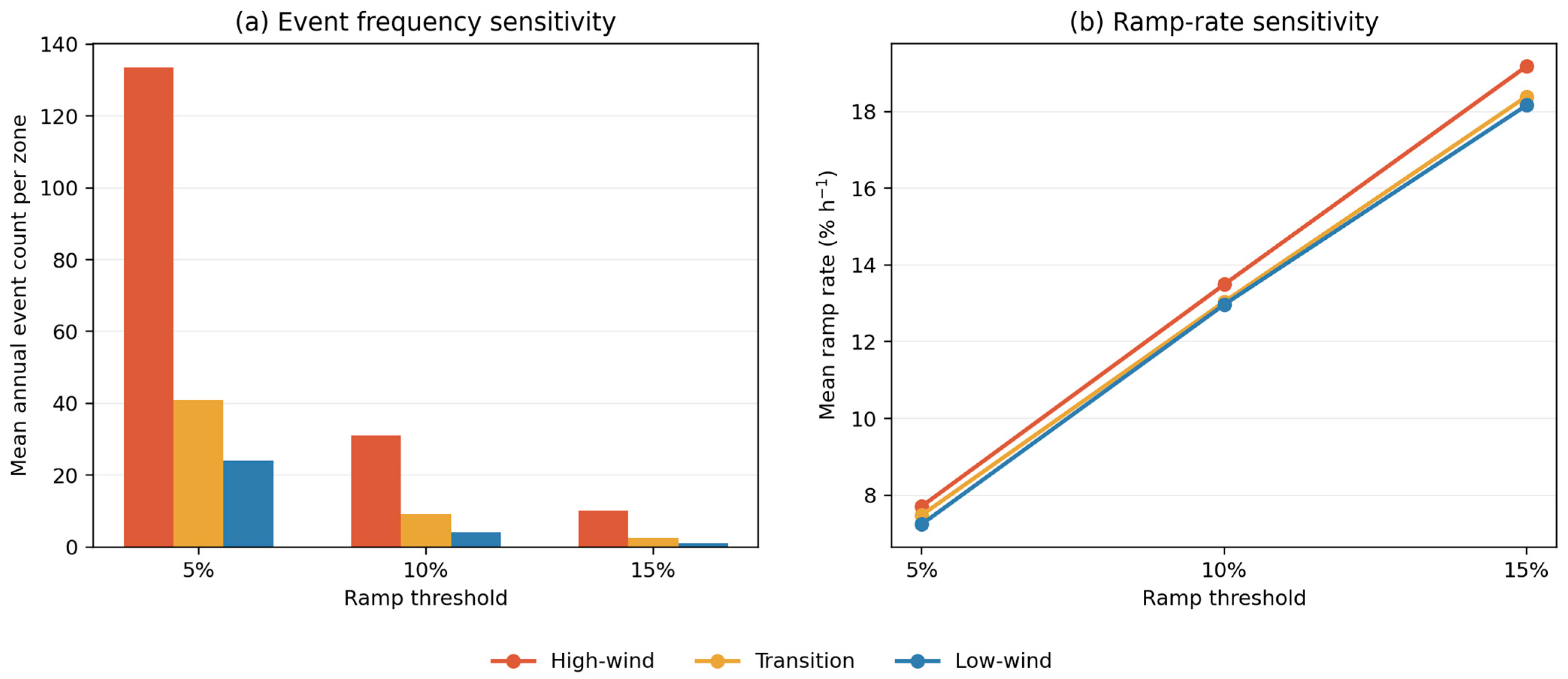
Figure 12 presents the sensitivity of wind power ramp event statistics to three capacity factor hourly change thresholds (5%, 10%, and 15%) across the high-wind, transition, and low-wind seasons. Figure 12a illustrates the decay in mean annual ramp event frequency with increasing threshold. At the 5% threshold, the zone-averaged annual event counts are 133.525, 40.856, and 24.128 for the high-wind, transition, and low-wind seasons, respectively. Raising the threshold to 10% reduces these values to 31.111, 9.228, and 4.108, representing relative decreases of 76.7%, 77.4%, and 83.0%. At the 15% threshold, counts decline further to 10.169, 2.550, and 1.031. Despite this order-of-magnitude reduction, the seasonal ranking of high-wind > transition > low-wind remains invariant across all thresholds. Figure 12b shows that the mean ramp rate increases approximately linearly with threshold. At 5%, mean ramp rates cluster within 7.243–7.711% h−1 across the three seasons. At 10%, rates rise to 13.492%, 13.041%, and 12.968% h−1 for the high-wind, transition, and low-wind seasons, respectively. At 15%, values reach 19.181%, 18.652%, and 18.164% h−1. The high-wind season consistently exhibits the highest ramp rate across all thresholds.

4. Discussion

The WRF validation (Figure 2 and Figure 3) reveals season- and zone-dependent biases that directly affect the reliability of downstream estimates. The domain-mean ME of +0.15 m·s−1 in the windy season is small relative to background wind speed, supporting reliable resource estimation during the primary production period. The calm season ME of +0.50 m·s−1 is more consequential. The calm season ME of +0.50 m·s−1 is more consequential for potential future applications, as any low-output risk assessment based on these data would need to account for the positive bias, which shortens apparent calm-period duration. This is particularly relevant for Z5 (ME +0.95 m·s−1) and Z8 (+0.76 m·s−1), where bias correction would be essential before operational use. Wind drought statistics in this study may therefore underestimate actual low-wind risk, particularly in Z5 (ME +0.95 m·s−1) and Z8 (+0.76 m·s−1). Conversely, Z2 (BYC) exhibits strong negative bias (−1.76 m·s−1 in the windy season), meaning its reported CF of ~0.127 is likely a lower bound of actual production potential. This underestimation stems from WRF’s inability to fully resolve narrow valley gap-flow acceleration at its grid spacing, a known limitation in complex terrain applications [23,24]. Season- and zone-specific bias correction should be applied before operational use of these results.
The spatial concentration of resources in a small number of terrain-controlled corridors (Figure 5) constrains geographic diversification of wind installations. Multiple wind farms within the same corridor share common meteorological forcing and are likely to produce highly correlated output. The same mechanism applies in Xinjiang, where major wind bases occupy collectively less than 5% of the total land area. The extreme seasonal asymmetry (Figure 6) compounds this constraint: Z5 concentrates 69% of annual EFLH in the windy season with a CF ratio of 5.2 between seasons. Heavy reliance on Z1 or Z5 without cross-seasonal storage would create persistent winter supply deficits. Z2 and Z6, whose calm season EFLH exceeds their transition season values, offer partial seasonal balancing. An optimal portfolio combining high-CF zones (Z1, Z7) with seasonally stable zones (Z2, Z6) would reduce required storage capacity, a topic warranting dedicated portfolio optimization analysis at the regional scale.
The trend results (Figure 7, Figure 8 and Figure 9) show that wind-speed evolution in Xinjiang is spatially differentiated rather than uniformly directional. Z2, Z3, Z5, and Z8 exhibit significant negative trends, consistent with the broader terrestrial stilling signal linked to increasing surface roughness and land-surface change [6,8,14]. By contrast, Z4 and Z6 show significant positive trends concentrated after 2006, consistent with the partial recovery reported for parts of Northwestern China after the 2000s [7]. The south–north divergence identified here likely reflects the combined influence of large-scale circulation variability, terrain channeling and shielding, and land-surface roughness change, instead of a single controlling factor. Northern Xinjiang, especially corridor and pass regions, is more directly affected by changes in the mid-latitude westerlies and regional pressure gradients, and thus may respond more strongly to decadal-scale circulation variability. Southern Xinjiang, particularly the Tarim Basin and the southern flank of the Tianshan Mountains, is more strongly influenced by topographic shielding, stable boundary layer conditions, and local land-surface effects, which may favor persistent decline in near-surface wind speed. The decadal decomposition (Figure 9) further shows that most long-term variability is concentrated in the high-wind season—Z1 low-wind WPD varies by only ~10 W·m−2 across four decades versus ~30 W·m−2 in the high-wind season—implying that variance budgets for energy yield estimation should be weighted toward the windy season.
Several limitations should be noted. The fixed WRF resolution cannot fully resolve sub-kilometer terrain features; gap-flow acceleration (Z2) and drainage flows (Z1) are underrepresented. The idealized cubic power curve neglects turbulence intensity, air density variation, and icing effects on real turbine performance. The 40-year record captures at most two complete decadal oscillation cycles, so identified trends may reflect low-frequency variability rather than monotonic change. Surface roughness is derived from GIMMS NDVI3g data (1981–2015 climatological mean) held constant over the full simulation period; actual roughness evolution due to urbanization and vegetation dynamics [6] is not modeled, future assessments should incorporate time-varying z0 derived from annual NDVI composites to isolate the contribution of land cover change to observed wind speed trends. In bare desert areas where NDVI approaches zero, the NDVI-z0 relationship may underrepresent mechanical roughness elements such as gravel ridges; future work could integrate high-resolution land surface datasets to refine z0 estimation in arid terrain. These interpretations are discussion-based and should not be regarded as a formal attribution, because the present analysis does not explicitly separate the relative contributions of circulation change, terrain effects, and land-surface processes. The ramp threshold is fixed at δ = 0.10 and conditional on assumed turbine specifications. Future work should incorporate time-varying land cover, higher-resolution simulations, and post-2018 data to test trend persistence, and should couple resource assessment with demand profiles and transmission constraints for system-level evaluation.

5. Conclusions

This study establishes three principal findings with implications for wind energy development in complex terrain regions.
  • Xinjiang’s wind energy is a terrain-locked resource, not a regional endowment. The domain-mean capacity factor of 0.08 confirms that the vast majority of the 1.66 million km2 territory has limited development value. Only the cores of Z1, Z7, and Z9 reach 3000–3900 equivalent full-load hours. This spatial concentration inherently constrains geographic diversification and implies persistently high output correlation among wind farms within the same corridor.
  • Long-term resource evolution is spatially differentiated and seasonally asymmetric. Southern and eastern zones show significant wind speed decline, while northern zones exhibit significant increases driven by post-2006 anomalies. Decadal variability originates almost entirely from the windy season; calm season output is approximately stationary across four decades. For project lifetime energy yield estimation, variance budgets should therefore be allocated predominantly to the April–August period. The diurnal capacity factor profiles—nocturnal peaks in basin-margin corridors, midday peaks in thermally driven passes—have remained phase-stable over 40 years (peak-time shifts within ±0.01 h), providing a reliable basis for dispatch scheduling and wind–solar complementarity design.
  • Extreme ramp events are seasonally exclusive to the windy season and spatially concentrated in Z1 and Z4, with declining frequency and intensity after 2006. This decoupling of mean wind speed trends from extreme event trends is favorable for grid stability: the resource gain in northern zones does not carry a proportional increase in ancillary service costs. These findings collectively support a zone-differentiated development strategy in which high-CF corridors supply bulk energy while seasonally stable zones reduce cross-seasonal storage requirements.

Author Contributions

Conceptualization, M.A. and J.T.; methodology, M.A. and J.T.; software, M.A. and Y.W.; validation, M.A., Y.W. and Y.A.; formal analysis, M.A. and Y.W.; investigation, M.A. and Y.A.; resources, J.T. and L.B.; data curation, M.A. and Y.W.; writing—original draft preparation, M.A.; writing—review and editing, J.T. and L.B.; visualization, M.A. and Y.W.; supervision, J.T. and L.B.; project administration, J.T.; funding acquisition, J.T. and L.B. All authors have read and agreed to the published version of the manuscript.

Funding

This research was funded by the Doctoral Research Start-up Fund of Changji University, grant number BSQD2026011.

Institutional Review Board Statement

Not applicable.

Informed Consent Statement

Not applicable.

Data Availability Statement

The GTOPO30 digital elevation model is publicly available from the U.S. Geological Survey (https://www.usgs.gov/centers/eros/science/usgs-eros-archive-digital-elevation-global-30-arc-second-elevation-gtopo30 (accessed on 27 May 2026)). The Global Inventory Modeling and Mapping Studies third-generation NDVI (GIMMS NDVI3g+) data are publicly available from the NASA ORNL Distributed Active Archive Center (https://doi.org/10.3334/ORNLDAAC/2187). Surface observation data from the Xinjiang Meteorological Information Center are subject to the data sharing policies of the China Meteorological Administration and are available upon request with appropriate authorization.

Acknowledgments

The Xinjiang Meteorological Information Center is acknowledged for providing quality-controlled surface wind speed observations. During the preparation of this manuscript, the authors used ChatGPT (OpenAI, GPT-5.4) for the purposes of improving language and editing text. The authors have reviewed and edited all output and take full responsibility for the content of this publication.

Conflicts of Interest

Author Y.A. is employed by Xinjiang Xinshui Kamarie Environmental Protection Technology Co., Ltd. The remaining authors declare that the research was conducted in the absence of any commercial or financial relationships that could be construed as potential conflicts of interest. The funder had no role in the design of the study; in the collection, analyses, or interpretation of data; in the writing of the manuscript; or in the decision to publish the results.

Abbreviations

The following abbreviations are used in this manuscript:
ATJAlataw Pass–Tacheng–Western Junggar Wind Corridor (Zone 9)
BNJBurqin–Northern Junggar Wind Zone (Zone 6)
BYCBarkol–Yiwu Core Wind Energy Zone (Zone 2)
CFCapacity Factor
EFLHEquivalent Full-Load Hours
HSESoutheastern Hami Wind Corridor (Zone 3)
NJTNortheastern Junggar Transitional Zone (Zone 4)
SCBSouthern Xinjiang Western–Central Basin Wind Belt (Zone 5)
TTCTurpan–Toksun Strong Wind Channel Zone (Zone 1)
UTDUrumqi–Tiechanggou–Dabancheng Wind Corridor (Zone 7)
WCBWestern-Central Intermountain Sheltered Basin Zone (Zone 8)
WPDWind Power Density
WSWind Speed
WS10Wind Speed of 10 m

Appendix A

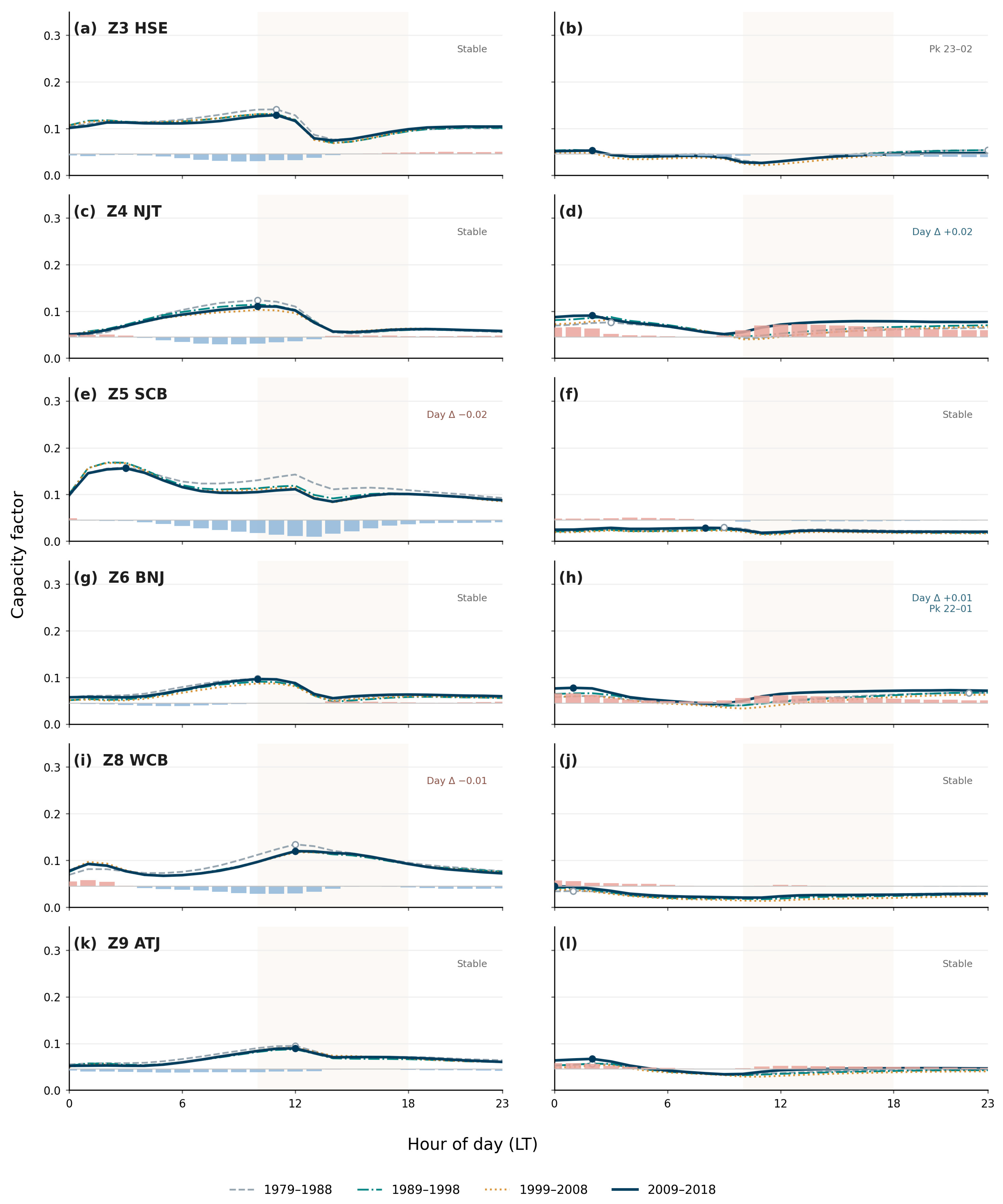
Figure A1 presents the diurnal CF evolution for six zones: Z3, Z4, Z5, Z6, Z8, and Z9. In the windy season (April–August), three distinct diurnal patterns emerge. The first is a midday single-peak type, shared by Z3 (HSE), Z4 (NJT), Z6 (BNJ), and Z9 (ATJ). CF peaks at 11:00–12:00 LST (approximately 0.13, 0.11, 0.10, and 0.09), then drops to 0.05–0.08 by 15:00–16:00 LST, yielding a diurnal range of 0.04–0.06. The second is a pre-dawn single-peak type, unique to Z5 (SCB). Output rises through the night and peaks at 03:00–04:00 LST (CF ~0.16), then declines through the daytime as thermal convection dissipates momentum, reaching a minimum of 0.09 at 16:00 LST. The third is a weak bimodal type at Z8 (WCB), with two peaks of similar magnitude at 02:00 LST (CF ~0.09) and 12:00 LST (CF ~0.12). In the calm season (November–February), Z5 and Z8 are compressed to CF 0.02–0.04 throughout the day, with negligible diurnal variation. Z4 and Z6 exhibit a seasonal phase reversal, where the peak shifts from midday to 01:00–02:00 LST (CF ~0.08–0.09), with a trough near 10:00 LST (CF ~0.04–0.05). Across all zones, peak-time shifts over four decades (Day Δ) remain within ±0.02 h. In terms of amplitude, Z5 and Z8 show decadal attenuation in the windy season; the daytime secondary peak CF of Z5 was approximately 0.14 in 1979–1988 but decreased below 0.11 in 2009–2018, confirming the long-term resource decline in the southern basin and western-central intermundane zones at the sub-daily scale.
Figure A1. Diurnal cycles of capacity factor at 100 m height for six wind zones (Z3, HSE; Z4, NJT; Z5, SCB; Z6, BNJ; Z8, WCB; and Z9, ATJ) in the windy (a,c,e,g,i,k) and low-wind (b,d,f,h,j,l) seasons. The four curves represent four decadal periods (1979–1988, 1989–1998, 1999–2008, and 2009–2018). Bottom bars show hourly capacity factor departures (ΔCF) from the daily mean. Annotated values (Day Δ) indicate temporal shifts in peak hours across the decades. Beige shading marks local daytime hours (10:00–18:00 LT).
Atmosphere 17 00649 g0a1

References

  1. IRENA. Renewable Power Generation Costs in 2022; International Renewable Energy Agency: Abu Dhabi, United Arab Emirates, 2023; Available online: https://www.irena.org/publications/2023/Aug/Renewable-Power-Generation-Costs-in-2022 (accessed on 15 May 2025).
  2. IEA. World Energy Outlook 2023; International Energy Agency: Paris, France, 2023; Available online: https://www.iea.org/reports/world-energy-outlook-2023 (accessed on 15 May 2025).
  3. GWEC. Global Wind Report 2024; Global Wind Energy Council: Brussels, Belgium, 2024. [Google Scholar]
  4. Pryor, S.C.; Barthelmie, R.J. Climate change impacts on wind energy: A review. Renew. Sustain. Energy Rev. 2010, 14, 430–437. [Google Scholar] [CrossRef]
  5. Petersen, E.L.; Mortensen, N.G.; Landberg, L.; Højstrup, J.; Frank, H.P. Wind power meteorology. Part I: Climate and turbulence. Wind Energy 1998, 1, 2–22. [Google Scholar] [CrossRef]
  6. Vautard, R.; Cattiaux, J.; Yiou, P.; Thépaut, J.-N.; Ciais, P. Northern Hemisphere atmospheric stilling partly attributed to an increase in surface roughness. Nat. Geosci. 2010, 3, 756–761. [Google Scholar] [CrossRef]
  7. Zeng, Z.; Ziegler, A.D.; Searchinger, T.; Yang, L.; Chen, A.; Ju, K.; Piao, S.; Li, L.Z.X.; Ciais, P.; Chen, D.; et al. A reversal in global terrestrial stilling and its implications for wind energy production. Nat. Clim. Change 2019, 9, 979–985. [Google Scholar] [CrossRef]
  8. McVicar, T.R.; Roderick, M.L.; Donohue, R.J.; Li, L.T.; Van Niel, T.G.; Thomas, A.; Grieser, J.; Jhajharia, D.; Himri, Y.; Mahowald, N.M.; et al. Global review and synthesis of trends in observed terrestrial near-surface wind speeds: Implications for evaporation. J. Hydrol. 2012, 416–417, 182–205. [Google Scholar] [CrossRef]
  9. Seguro, J.V.; Lambert, T.W. Modern estimation of the parameters of the Weibull wind speed distribution for wind energy analysis. J. Wind Eng. Ind. Aerodyn. 2000, 85, 75–84. [Google Scholar] [CrossRef]
  10. Hersbach, H.; Bell, B.; Berrisford, P.; Hirahara, S.; Horányi, A.; Muñoz-Sabater, J.; Nicolas, J.; Peubey, C.; Radu, R.; Schepers, D.; et al. The ERA5 global reanalysis. Q. J. R. Meteorol. Soc. 2020, 146, 1999–2049. [Google Scholar] [CrossRef]
  11. Gelaro, R.; McCarty, W.; Suárez, M.J.; Todling, R.; Molod, A.; Takacs, L.; Randles, C.A.; Darmenov, A.; Bosilovich, M.G.; Reichle, R.; et al. The Modern-Era Retrospective Analysis for Research and Applications, Version 2 (MERRA-2). J. Clim. 2017, 30, 5419–5454. [Google Scholar] [CrossRef] [PubMed]
  12. Jung, C.; Schindler, D. A review of recent studies on wind resource projections under climate change. Renew. Sustain. Energy Rev. 2022, 165, 112596. [Google Scholar] [CrossRef]
  13. Staffell, I.; Pfenninger, S. Using bias-corrected reanalysis to simulate current and future wind power output. Energy 2016, 114, 1224–1239. [Google Scholar] [CrossRef]
  14. Wu, J.; Zha, J.; Zhao, D.; Yang, Q. Changes in terrestrial near-surface wind speed and their possible causes: An overview. Clim. Dyn. 2018, 51, 2039–2078. [Google Scholar] [CrossRef]
  15. Chen, L.; Li, D.; Pryor, S.C. Wind speed trends over China: Quantifying the magnitude and assessing causality. Int. J. Climatol. 2013, 33, 2853–2864. [Google Scholar] [CrossRef]
  16. Ouyang, T.; Kusiak, A.; He, Y. Modeling wind-turbine power curve: A data partitioning and mining approach. Renew. Energy 2017, 102, 1–8. [Google Scholar] [CrossRef]
  17. Rose, S.; Apt, J. The cost of curtailing wind turbines for secondary frequency regulation capacity. Energy Syst. 2014, 5, 407–422. [Google Scholar] [CrossRef]
  18. Potisomporn, P.; Vogel, C.R. Spatial and temporal variability characteristics of offshore wind energy in the United Kingdom. Wind Energy 2022, 25, 537–552. [Google Scholar] [CrossRef]
  19. Zhu, R.; He, X.F.; Zhou, R.W. Detailed Assessment of Wind Energy Resources in China; China Meteorological Press: Beijing, China, 2014. (In Chinese) [Google Scholar]
  20. Zhang, T.; Wang, H.; Yu, X. Spatial-temporal distribution characteristics of wind disasters in Xinjiang. Arid Land Geogr. 2021, 44, 1281–1289. (In Chinese) [Google Scholar] [CrossRef]
  21. He, Q.; Yuan, Y.J.; Wei, W.S. Assessment of wind energy resources in Xinjiang. Arid Land Geogr. 2010, 33, 174–182. (In Chinese) [Google Scholar]
  22. Ren, G.Y.; Guo, J. Change in wind speed over mainland China: An overview. Acta Meteorol. Sin. 2006, 64, 680–691. (In Chinese) [Google Scholar]
  23. Zhu, R.; Zhang, H.; He, C.; Wu, Z.; Dai, J.; Chen, B.; Liu, J.; Bai, L. High-resolution assessment of wind energy potential and operational risks in complex mountain-basin systems. Atmosphere 2025, 16, 1362. [Google Scholar] [CrossRef]
  24. Bai, L.; Shang, M.; Shi, C.; Bian, Y.; Liu, L.; Zhang, J.; Li, Q. Spatiotemporal wind speed changes along the Yangtze River Waterway (1979–2018). Atmosphere 2026, 17, 81. [Google Scholar] [CrossRef]
  25. Xu, J.; Wu, J.; Xing, Y.; Yang, D.; Jiao, Y.; Shang, M.; Bai, L. Wind speed error analysis of high spatiotemporal resolution land surface variable reanalysis products over China. Clim. Change Res. Lett. 2025, 14, 831–841. (In Chinese) [Google Scholar] [CrossRef]
  26. Pinzon, J.E.; Tucker, C.J. A non-stationary 1981–2012 AVHRR NDVI3g time series. Remote Sens. 2014, 6, 6929–6960. [Google Scholar] [CrossRef]
  27. Bastiaanssen, W.G.M.; Menenti, M.; Feddes, R.A.; Holtslag, A.A.M. A remote sensing surface energy balance algorithm for land (SEBAL). 1. Formulation. J. Hydrol. 1998, 212–213, 198–212. [Google Scholar] [CrossRef]
  28. Gualtieri, G. A comprehensive review on wind resource extrapolation models applied in wind energy. Renew. Sustain. Energy Rev. 2019, 102, 215–233. [Google Scholar] [CrossRef]
  29. Justus, C.G.; Mikhail, A. Height variation of wind speed and wind distributions statistics. Geophys. Res. Lett. 1976, 3, 261–264. [Google Scholar] [CrossRef]
  30. IEC 61400-12-1; Wind Energy Generation Systems—Part 12-1: Power Performance Measurements of Electricity Producing Wind Turbines. International Electrotechnical Commission (IEC): Geneva, Switzerland, 2017.
  31. Willmott, C.J. On the validation of models. Phys. Geogr. 1981, 2, 184–194. [Google Scholar] [CrossRef]
Figure 1. Overview of the study area and intra-annual wind speed variations. (a) Geographical location, complex topography (terrain rendered from GTOPO30), meteorological stations (105 long-term stations, indicated by red dots), and nine sub-regions delineated for wind energy assessment across Xinjiang. (b) Monthly variations in mean wind speed (WS, m·s−1) across the nine sub-regions and Xinjiang (XJ) from January to December. The base map of Xinjiang is sourced from the standard map with approval number GS(2019)1822.
Atmosphere 17 00649 g001
Figure 2. Mean error (a), root mean square error (b), and correlation coefficient (c) of WRF-simulated wind speed across Xinjiang, stratified by wind season (1979–2018).
Atmosphere 17 00649 g002
Figure 3. Heatmaps of mean error (a), root mean square error (b), and correlation coefficient (c) for WRF-simulated wind speed across nine wind zones (Z1–Z9), stratified by wind season.
Atmosphere 17 00649 g003
Figure 4. Spatial distribution of the evaluation metrics for WRF-simulated near-surface wind speed against 105 meteorological stations in Xinjiang during the period of 1979–2013 (based on 00, 06, 12, and 18 UTC data). Subplots indicate: (a) root mean square error (RMSE, m·s−1), (b) correlation coefficient (r), and (c) bias (m·s−1).
Atmosphere 17 00649 g004
Figure 5. Climatological spatial distribution of annual mean wind speed (a), wind power density (b), capacity factor (c), and equivalent full-load hours (d) at 100 m height across Xinjiang (1979–2018).
Atmosphere 17 00649 g005
Figure 6. Seasonal comparison of mean capacity factor (a) and equivalent full-load hours (b) across nine wind zones during high-wind, transition, and calm seasons. Error bars indicate interannual standard deviation.
Atmosphere 17 00649 g006
Figure 7. Spatial distribution of linear trends in 100 m wind speed (a) and wind power density (b) across Xinjiang (1979–2018). Positive values indicate enhancement; negative values indicate weakening.
Atmosphere 17 00649 g007
Figure 8. Interannual anomaly heatmaps of 100 m wind speed (a) and wind power density (b) for Xinjiang (XJ) and nine wind zones (1979–2018). Right-side bar charts show linear trends; asterisks indicate Mann–Kendall significance at p < 0.05.
Atmosphere 17 00649 g008
Figure 9. Decadal trajectories of 100 m wind speed (a) and wind power density (b) across nine wind zones, and their seasonal decomposition for the high-wind and calm seasons (c,d).
Atmosphere 17 00649 g009
Figure 10. Diurnal cycles of capacity factor at 100 m height for Xinjiang (XJ) and zones Z1 (TTC), Z2 (BYC), and Z7 (UTD) in the high-wind (a,c,e,g) and low-wind (b,d,f,h) seasons. Four curves represent four decadal periods; bottom bars show hourly ΔCF departures. Beige shading marks local daytime hours (10:00–18:00 LT).
Atmosphere 17 00649 g010
Figure 11. Interannual anomaly heatmaps of extreme wind power ramp events across nine zones in high-wind, transition, and calm seasons (1979–2018): event frequency (a), mean ramp rate (b), and maximum shock intensity (c).
Atmosphere 17 00649 g011
Figure 12. Sensitivity analysis of wind power ramp events under different hourly capacity factor change thresholds (5%, 10%, and 15%). (a) Mean annual event count per zone and (b) corresponding mean ramp rate (% h−1) across high-wind, transition, and low-wind regimes.
Atmosphere 17 00649 g012
Disclaimer/Publisher’s Note: The statements, opinions and data contained in all publications are solely those of the individual author(s) and contributor(s) and not of MDPI and/or the editor(s). MDPI and/or the editor(s) disclaim responsibility for any injury to people or property resulting from any ideas, methods, instructions or products referred to in the content.