Article

Validation of the 2021 Emission Inventory for Cuenca, Ecuador, Through Weather and Air Quality Modeling in the Framework of WRF-Chem

1
Instituto de Simulación Computacional (ISC-USFQ), Colegio de Ciencias e Ingenierías, Universidad San Francisco de Quito (USFQ), Quito 170901, Ecuador
2
Red de Monitoreo de Calidad del Aire de Cuenca, Empresa Pública de Movilidad, Tránsito y Transporte de Cuenca, EMOV EP, Cuenca 010206, Ecuador
*
Author to whom correspondence should be addressed.
Atmosphere 2026, 17(6), 569; https://doi.org/10.3390/atmos17060569
Submission received: 21 March 2026 / Revised: 10 May 2026 / Accepted: 28 May 2026 / Published: 31 May 2026
(This article belongs to the Special Issue Emission Inventories and Modeling of Air Pollution)

Abstract

The last atmospheric emission inventory for Cuenca, a city located in the Andean region of southern Ecuador, was developed for the year 2021 (EI 2021) and encompasses both primary pollutants (NOx, CO, VOC, SO2, PM10, and PM2.5) and greenhouse gases (CO2, CH4, and N2O). We formally assessed the quality of this emission inventory by modeling air quality levels in October 2021 using the Weather Research and Forecasting with Chemistry (WRF-Chem 3.2) model at a high spatial resolution (1 km). Although we conducted simulations with different combinations of boundary conditions for chemical species and hourly profiles to disaggregate daily on-road traffic emissions, we selected two sets of numerical experiments to report. The results indicated that most of the assessed meteorological and air quality variables were modeled acceptably, suggesting that the EI 2021 emission inventory is a reasonable estimation of real emissions. The results also indicated the current capacity of WRF-Chem to model the atmosphere in a complex Andean city using the “one atmosphere” approach, highlighting the variables with good, fair, and poor modeling performance. We propose future research directions to improve emission inventories and the performance of atmospheric modeling in the Equatorial Andean region. Finally, the results and spatial distribution of the EI 2021 were compared to the emission data from the last version of the EDGAR Emissions Dataset (which has a spatial resolution of 11.1 km), one of the most used global emission datasets. We concluded that, for the Equatorial Andean region and for modeling purposes, the EDGAR Dataset results should be reviewed, both to account for the effects of height above sea level on the magnitude of primary pollutant emissions and their spatial configuration.

1. Introduction

Atmospheric emission inventories provide relevant information on the amount or rates of air pollutant and greenhouse gas (GHG) emissions produced by different sources over a specific region in the past, present, or future [1,2]. Atmospheric emission inventories have been used both for policy and research purposes. They provide temporal behavior data that can be used to track the progress in achieving reductions in emissions, e.g., refs. [3,4]. On the other hand, emission inventories provide input for chemical transport models, which simulate the behavior of pollutants in the atmosphere for both current and hypothetical emission scenarios, as well as for atmospheric forecasting [5,6,7]. Emission data are probably the most important input for chemical transport models [8].
The building and use of accurate atmospheric emission inventories are directly related to several Sustainable Development Goals (SDGs), such as SDG 3 (Good Health and Well-Being), by identifying the main air pollution sources and guiding air quality regulations; SDG 11 (Sustainable Cities and Communities), by supporting city-level policies for cleaner transport, energy, and waste management; and SDG 13 (Climate Action), by quantifying GHGs and other pollutants involved in the energetic balance of the atmosphere, identifying their emissions sources and sinks, and tracking mitigation progress [9].
International initiatives aim to develop and make the results of emission inventories available to inform scientists and policymakers. The EDGAR Emissions Database for Global Atmospheric Research is a dataset that covers time-series emission inventories for anthropogenic sources of primary pollutants and GHGs for all countries, with a spatial resolution of up to 0.1° (approximately 11.1 km) [10]. The EDGAR Emissions Database is one of the most widely used global atmospheric emission inventories, providing, in addition to annual estimation of primary pollutants and GHGs, temporal profiles for disaggregating annual emissions into monthly and hourly data by country and emission source. The CAMS emission inventory contains gridded distributions of global anthropogenic and natural emissions of atmospheric pollutants and GHGs, with a resolution of up to 0.1° [11].
Although emission inventories have been developed for many years, they still can have high levels of uncertainty [12,13,14]. Apart from the uncertainties inherent in emission models as simplifications of real emissions, other factors, such as the limitations of statistical data and the lack of local emission factors, can also significantly contribute. Uncertainty is also influenced by the method used to downscale total emission results to a grid-cell level, which is accompanied by high-time resolution disaggregation in order to use the data in a chemical transport model [15]. An assessment of uncertainty is required to clarify the usefulness of emission inventories and identify the sources that should be targeted in the future [16].
The quality of an emission inventory has typically been defined by the quality of the statistical data, emission factors, and models used in its development. Additionally, when available, it should be compared with other emission inventories. Another approach to assessing the quality of an emission inventory is to use it as input for atmospheric modeling. Mathias et al. (2017) [8] highlighted the need to work with accurate emissions data and provided an outlook for improving the spatial and temporal distribution of emissions inventories for use in chemical transport models. Park et al. (2023) [14] assessed emission inventories for sulfur dioxide (SO2) and nitrogen oxides (NOx) from large point sources in South Korea, evaluating the modeling performance through a comparison of computed and recorded data for these pollutants. Malasani et al. (2024) [17] assessed five global emission inventory datasets to determine the spatial and temporal distribution of mercury over India and also evaluated the modeling performance by comparing modeled and measured concentrations of this pollutant.
Online coupled meteorology–atmospheric chemistry models, which consider the influence and feedback between atmospheric and air quality variables, have undergone significant evolution in recent years [18]. The online approach provides consistent treatment of physical and chemical processes for both numerical weather and air quality modeling, allowing for a “one atmosphere” approach to the analysis. If the meteorological component is properly modeled and the comparison of the modeled air pollution levels with the corresponding records indicates consistency, we can deduce that the emission inventory is reliable and provides useful information, though with some uncertainties.
For Cuenca, a city located in the Andean region of southern Ecuador, several emission inventories have been developed since 2007. The results of the 2014 emission inventory [19] were used to conduct several modeling experiments to assess the influence of the parameters and options coded in the Weather Research and Forecasting with Chemistry (WRF-Chem 3.2) model. These numerical experiments employed the online option and proposed a configuration of parameters for modeling both meteorological and air quality variables using the “one atmosphere” approach [20,21] in urban areas of the Equatorial Andean region.
The last emission inventory for this city was created using 2021 as the base year [22], which is hereafter referred to as the EI 2021. Although its uncertainty was assessed, the purpose of this contribution is to evaluate the quality and usefulness of the EI 2021 by incorporating its results as input to WRF-Chem for “one atmosphere” modeling of both meteorological and air quality variables. Additionally, the EI 2021 results are compared with the corresponding results from the EDGAR Emissions Dataset.

1.1. Location and the Air Quality-Monitoring Network of Cuenca

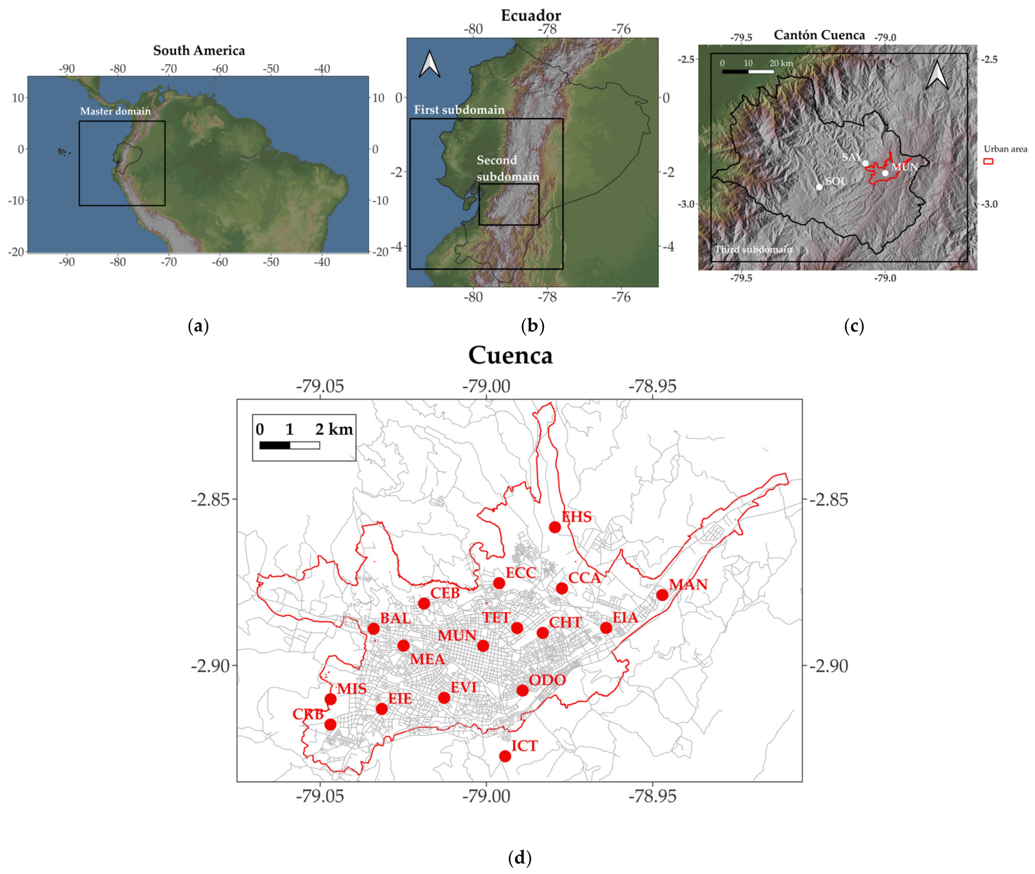
Cuenca, located in the Andean region of southern Ecuador (Figure 1), is characterized by a complex topography and diverse land-use configuration. The urban area is located at 2550 masl; however, the Andes Mountains, to the west of the city, have heights exceeding 4000 masl (Figure 1c). Its air quality-monitoring network has been operational since 2008, in accordance with national regulations. Currently, the air quality-monitoring network is operated by the EMOV EP (Empresa Pública Municipal de Movilidad, Tránsito y Transporte de Cuenca). Between 2012 and 2024, the MUN station (the city’s historic center) measured yearly mean PM2.5 concentrations; they were found to range between 5.7 and 14.5 µg m−3 [23], which is higher than the current World Health Organization (WHO) recommendation (5.0 µg m−3) [24]. Typically, O3 levels are highest in September and October, mainly due to the elevated solar radiation, and in some years, forest fires contribute to O3 precursor emissions. More information about the air quality-monitoring network is included in Appendix A.1.

1.2. The Emission Inventory of the Year 2021 (EI 2021)

The last atmospheric emission inventory for Cuenca was compiled for the year 2021 by the EMOV EP [25] in accordance with the recommended practice of accounting for primary pollutants and GHGs [13]. Nitrogen oxides (NOx), carbon monoxide (CO), volatile organic compounds (VOCs), sulfur dioxide (SO2), and particulate matter with an aerodynamic diameter of 10 µm or less (PM10) and 2.5 µm or less (PM2.5) were included as primary pollutants. In addition, carbon dioxide (CO2), methane (CH4), and nitrous oxide (N2O) were included as GHGs.
Sources included on-road traffic, vegetation, industries, use of solvents, service stations, domestic combustion of liquid petroleum gas (LPG), air traffic, landfills, artisanal production of bricks, dust resuspension, and mining activities in the territory of the Cantón Cuenca (Figure 1c).
The EI 2021 was developed to estimate real emissions as accurately as possible in the territory of Cuenca, with the main goals of providing a proper emission inventory that can serve as a reference for air pollution management and the development of a future atmospheric forecasting system. The EI 2021 includes hot, cold, and evaporative emissions from on-road traffic [26], the VOC emissions from vegetation (based on the model by Guenther et al. [27,28]), and emissions from landfills [29].
The EI 2021 was published as a technical report [25]. More information on the EI 2021 is provided in Appendix A.2.

2. Methods

2.1. Modeling Approach

Using WRF-Chem 3.2 [30], previous modeling experiments were conducted for Cuenca to analyze the influence of planetary boundary layer, land-surface, cumulus, and microphysics schemes [20,21]. Based on these studies, the recommended set of schemes and options for modeling both atmospheric and air-quality variables (Table 1) was used to validate the EI 2021. WRF-Chem is a state-of-the-art numerical 3D model used for research and forecasting purposes that enables online analysis by considering interactions between meteorological and air quality variables through the “one atmosphere” approach.
First, a master domain which covers the entire Ecuadorian continental territory (grid of 70 × 70, 27 km cells; Figure 1a) and two nested subdomains (Figure 1b) (first subdomain: 52 × 52, 9 km cells; second subdomain: 61 × 42, 3 km cells) were used to conduct the meteorological simulations from 1 to 30 of October 2021. A third and inner subdomain of 100 × 82 cells (1 km on each side) covering the territory of Cuenca (Figure 1d), which corresponds to the grid used for the development of EI 2021, was used to simulate meteorological and air quality variables. For vertical resolution, we used 35 vertical levels up to a top pressure of 50 hPa (altitude of approximately 20 km). The initial and boundary conditions were generated using the Global Operational Analysis (Final, FNL) [31]. The Carbon Bond Mechanism Z (CBMZ) [32] and the Model for MOSAIC (4 sectional aerosol bins) [33] were selected to speciate and represent the corresponding hourly emissions of gaseous pollutants and aerosols, respectively. The online option accounts for the direct effects of feedback between aerosols and meteorological variables.
To test the quality of the emission inventory and considering both the availability of records and pollution conditions, we selected October 2021 for modeling, which was the month with the highest O3 records of that year [34] and had representative socioeconomic activities related to atmospheric emissions for most of that year. Typically, the maximum levels of O3 occur in Cuenca during September and October, in part due to the highest surface solar radiation, which promotes VOCs emissions from both vegetation and anthropogenic sources, thereby promoting photochemical reactions. In addition, during these months, on-road traffic levels, both from gasoline and diesel vehicles, are high due to the reactivation of labor and academic activities after vacation.
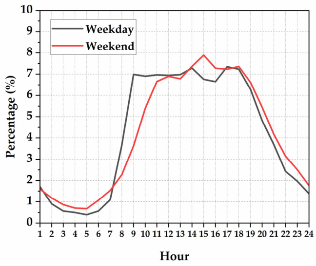
On-road traffic emissions for October were estimated as a fraction of annual emissions using the ratio of October gasoline and diesel sales to total fuel sales at all service stations in Cuenca in 2021. Based on EMOV EP estimates of weekday-to-weekend traffic dynamics, we assumed 80% and 60% of weekday traffic on Saturdays and Sundays, respectively. These percentages were previously used and yielded coherent results when assessing the influence of parameters and schemes on the set of options listed in Table 1, which was used in this contribution.
Previous modeling exercises using WRF-Chem 3.2 in Ecuadorian cities indicated that the default VOC vertical profile would be higher for the Ecuadorian Andean region. Therefore, it was necessary to decrease the vertical concentrations originally coded in the model. In addition, because the magnitude of hourly emissions also affects modeling performance, we conducted various numerical experiments. From these results, we selected two sets of numerical experiments to report in this manuscript:
  • Numerical Experiment 1 (NE 1): boundary conditions for chemical species for the inner domain were assumed to be 80% of the default concentrations specified in WRF-Chem V3.2. We used two basic hourly traffic profiles from the EMOV EP to characterize weekday and weekend on-road emissions.
  • Numerical Experiment 2 (NE 2): boundary conditions for chemical species for the inner domain were assumed to be 70% of the default concentrations specified in WRF-Chem V3.2. For this experiment, we used the hourly traffic profile from the EMOV EP for weekdays and the hourly traffic profile from the EDGAR Dataset for Ecuador for weekends on-road emissions.
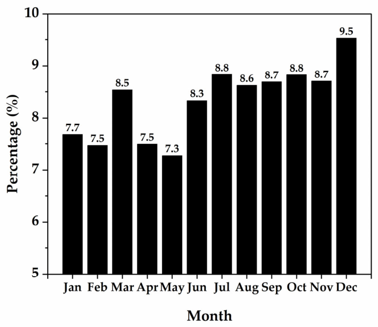
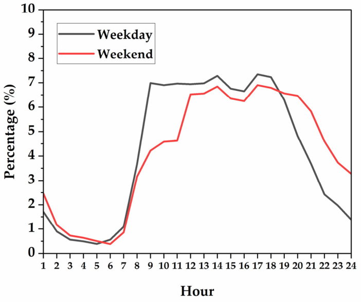
Appendix A.3 includes figures of the percentages used to estimate monthly and hourly on-road emissions for modeling.
Vegetation emissions were estimated on an hourly basis using the meteorological component of WRF-Chem for each day of October to simulate temperature and photosynthetically active radiation for each cell of the inner subdomain (1 km resolution). Emissions from combustion from large industrial facilities were assumed to be constant with a fixed hourly pollutant emission rate.
We conducted simulations for three-day periods, using six hours of spin-up time for each, and initialized the chemistry using the default WRF-ChemV3.2 idealized profile.
Table 1. Schemes and options for atmospheric modeling in the Ecuadorian Andean region [20,21].
ComponentWRF VariableOptionModel and References
Cumulus Parameterizationcu_physics00 No Cumulus
Microphysicsmp_physics3WRF Single–moment 3–class [35]
Longwave Radiationra_lw_physics1RRTM [36]
Shortwave Radiationra_sw_physics2Goddard [37]
Surface Layersf_sfclay_physics1MM5 similarity [38]
Planetary Boundary Layerbl_pbl_physics1Yonsei University [39]
Land Surfacesf_surface_physics2Noah [40]
Urban Surfacesf_urban_physics0No urban physics
Chemical Mechanism and Aerosol Moduleschem_opt7CBMZ and MOSAIC [32,33]

2.2. Metrics for Modeling Performance

We assessed the performance of the model in predicting the hourly surface temperature and hourly wind speed using the following metrics [41]:
G E = 1 N i = 1 N P i O i
M B = 1 N i = 1 N P i O i
I O A = 1 i = 1 N P i O i 2 i = 1 N P i P m + O i O m 2
R M S E = 1 N i = 1 N P i O i 2
  • GE: gross error, which measures the magnitude of the difference between modeled and observed values, regardless of whether the modeled values are higher or lower than the observed values.
    MB: mean bias, which quantifies the tendency of the model to over- or underestimate the values.
    IOA: index of agreement, which measures the degree to which the modeled values match the records, considering both the variance and magnitude of the differences.
    RMSE: root mean square error, which measures the overall difference between the model and the records, with a greater weight on significant differences.
    N: number of values.
    Pm: mean model value.
    Om: mean observed value.
    Pi: model value.
    Oi: record.
Table 2 indicates the ideal ranges and expected accuracies for these metrics, as suggested in [41], about the application of models under the European Union’s Air Quality Directive, which emphasizes the use of models combined with monitoring data for a range of applications about air quality management.
The model’s performance for daily rainfall was assessed using Equation (5).
P d c m = N d r + N d w r T m d · 100
  • Pdcm: percentage of days with or without rainfall from model.
    Ndr: number of days with rainfall (≥0.2 mm d−1) in both records and model results.
    Ndwr: number of days without rainfall (<0.2 mm d−1) in both records and model results.
    Tmd: total number of modeled days.
A rainfall intensity of 0.2 mm d−1 was used to define a rainy day or a day with measurable precipitation [42]. For days without rainfall, we considered that the model captured the record if both were <0.2 mm d−1. For days with rainfall, we considered the model to agree with the corresponding record if both values were ≥0.2 mm d−1.
To assess the short-term air quality modeling performance, we used the hourly records for nitrogen dioxide (NO2), PM2.5, and O3 from the MUN station to deduce the concentrations of these pollutants during specified periods of time (Table 2), according to national regulation and the WHO guidelines [24,43,44]. We considered the days having more than 70% of the corresponding hourly records. Based on Simon et al. (2012) about metrics used for air quality modeling [45], the last concentrations were used to compute the MB, RMSE, and the correlation coefficient (r):
r = 1 N i = 1 N O i O m P i P m 1 N i = 1 N O i O m 2 1 N i = 1 N P i P m 2
  • r measures the strength of the linear relationship between the modeled and observed values.
To assess the long-term air quality model’s performance, we calculated the percentage of passive stations with a difference of less than 30% between modeled monthly concentrations and recorded data. Additionally, we calculated the percentage of records correctly predicted by the model based on the accuracy presented in Table 2.
Table 2. Metrics for modeling atmospheric variables [41,45].
VariableMetricBenchmark or
Ideal Range
Accuracy
Hourly surface temperatureGE<2 °C±2 °C
MB(−0.5 °C, 0.5 °C)
IOA≥0.8
Hourly wind speed (10 mas)RMSE<2 m s−1±1 m s−1
MB(−0.5 m s−1, 0.5 m s−1)
IOA≥0.6
Daily air quality: 24 h NO2 mean, 24 h PM2.5 mean, max. 8 h O3 meanMB0±50%
RMSE0
r1
Monthly air quality: NO2 and O3 ±30%

2.3. Processing of the Data from the EDGAR Emissions Database

For comparison purposes, we identified and extracted information from cells within the global domain of the EDGAR Emissions Database (EDGARv8.1) [4,10,15,46] mesh covering the territory of the Cantón Cuenca (Figure 1c). We geoprocessed the EDGAR emission data for the year 2021. We totaled the emissions from these cells in the EI 2021 for the corresponding primary pollutants and GHGs.

3. Results

3.1. Meteorology

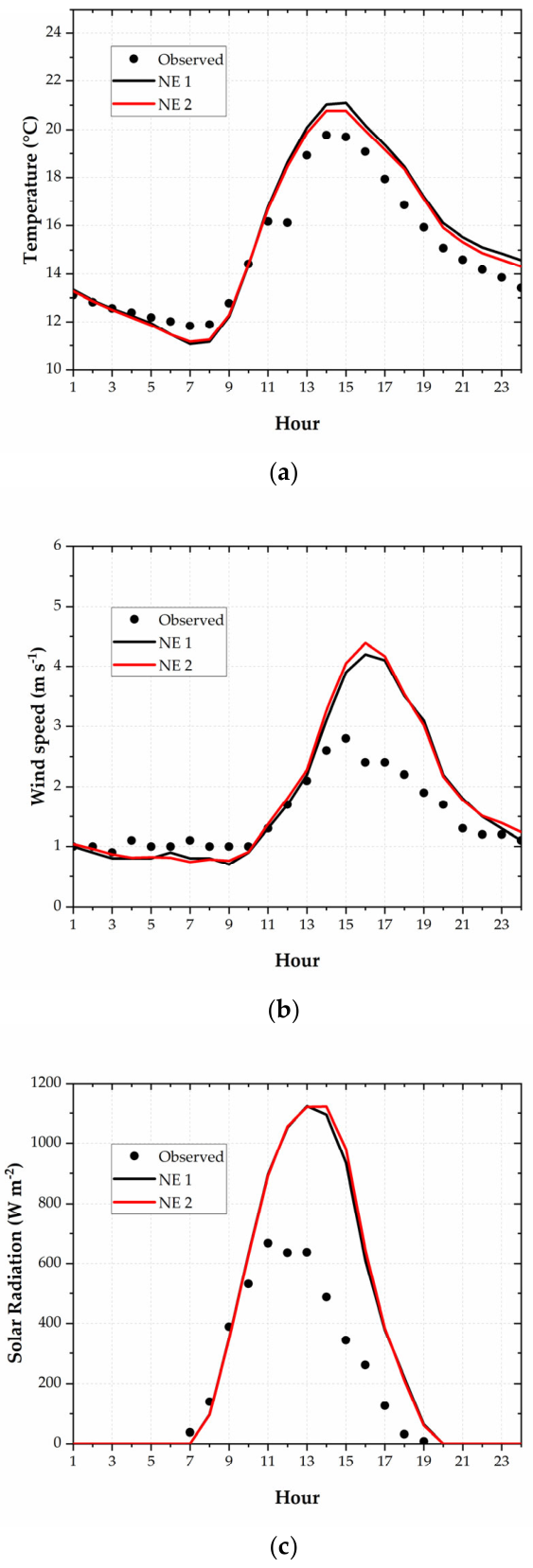
At the MUN station, although the model overestimated the surface temperature (MB = 0.61 °C for the NE 1 and 0.49 °C for the NE 2), the GE (1.46, 1.54 °C) and IOA (0.84, 0.83) were within the expected benchmark ranges for the two sets of experiments (Table 3), indicating that the model captured the trends of the records (Figure 2a). However, at the SAY station, both the GE (2.11, 2.18 °C) and MB (0.74, 0.62 °C) were out of range. For both stations and the two sets of experiments, the model provided a close match between the records and modeled hourly temperatures (IOA ≥ 0.8).
At the MUN station, although the model showed a slight overestimation during afternoons (Figure 2b), the wind speed was acceptably modeled as all the metrics fell within the expected ranges (Table 3).
The model correctly predicted 78.4% and 60.3% of the hourly temperature records at the MUN and SAY stations, respectively, for the NE 1 (Table 4). These percentages decreased to 77.4% and 58.9%, respectively, for the NE 2. Most of the wind speed records at the MUN station (75.8, 76.1%) were modeled adequately.
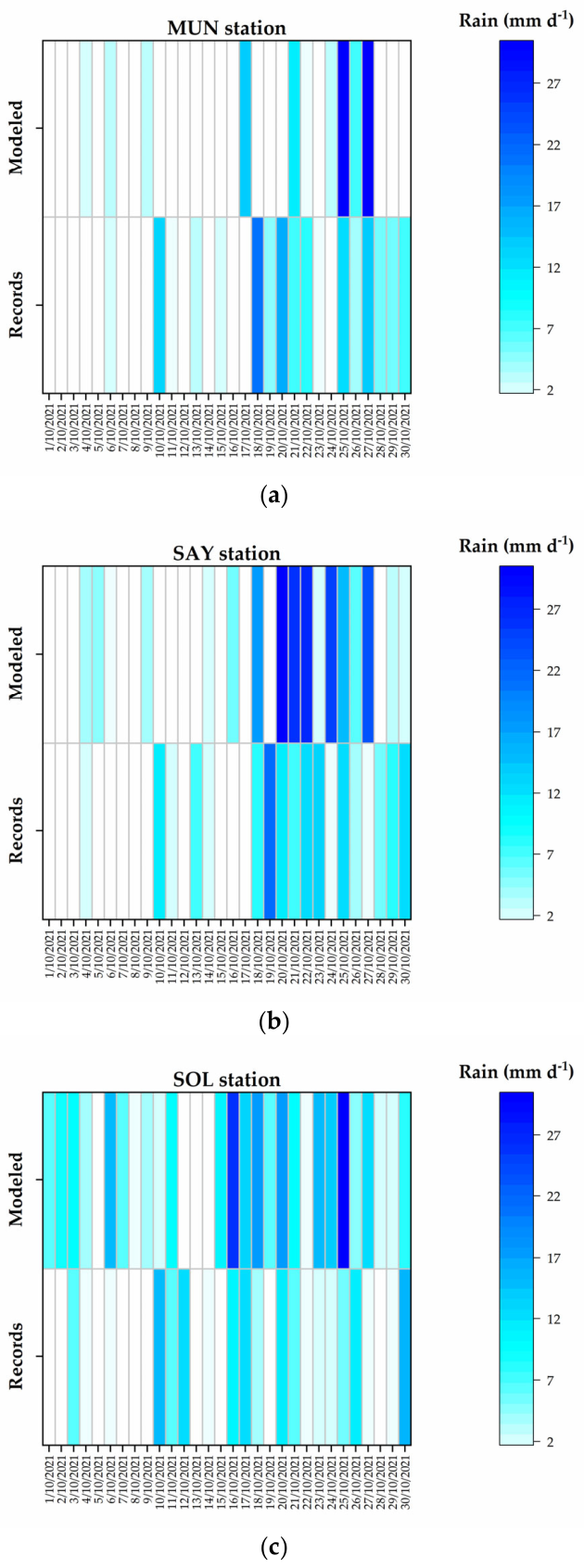
The model showed the highest accuracy for daily rainfall at the SAY station (80.0, 73.3%), followed by the SOL station (73.3, 66.7%) and the MUN station (46.7, 55.7%).
From 1 to 30 October 2021, 19 days had no rainfall or intensities lower than or equal to 0.2 mm d−1 at the MUN station (Figure 3a). Eleven days showed measurements between 0.4 and 21.0 mm d−1. In comparison, for the NE 1, the model identified 13 days with no rainfall or intensities lower than or equal to 0.2 mm d−1 and 17 days with intensities between 0.4 and 30.5 mm d−1. A better agreement was obtained at the SAY station, which had 20 days without rainfall or with rainfall intensities lower than or equal to 0.2 mm d−1, similar to the days quantified by the model. At the SOL station, which is located over the Andean mountains, the model indicated that all the days (30) had intensities higher than 0.2 mm d−1 while the records indicated 22 days. At the three stations, the ranges of the modeled rainfall were consistent with the ranges of the records.
The global solar radiation at the SOL (Figure 2c) and SAY was overestimated for the two numerical experiments.

3.2. Air Quality

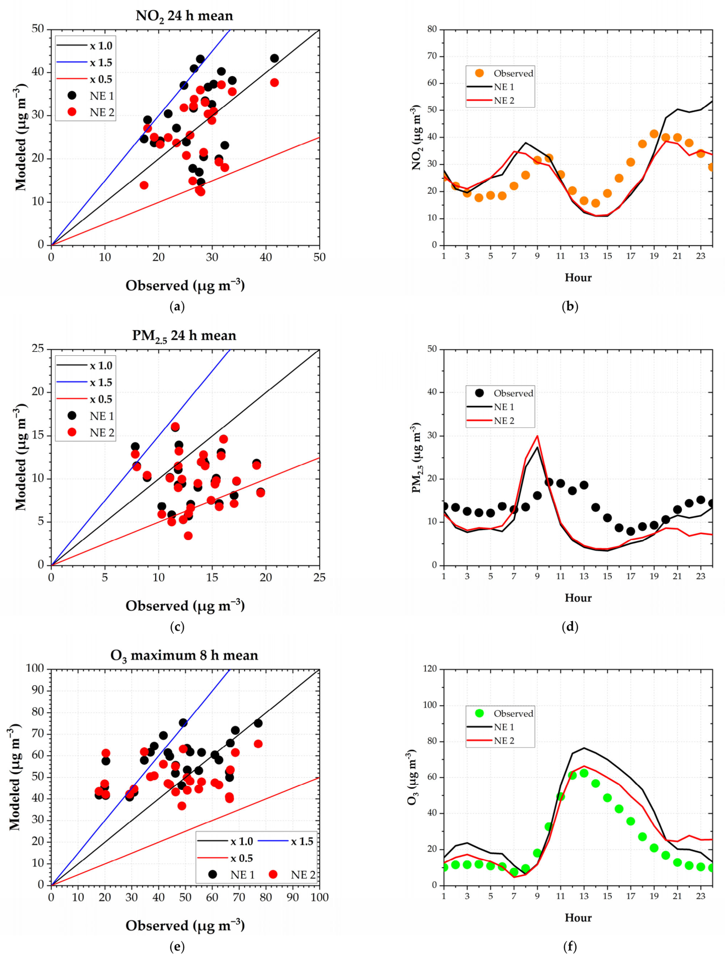
Although the model provided a mean daily profile consistent with the records, it slightly overestimated the mean 24 h NO2 levels (MB = 1.1 µg m−3) for the NE 1 but underestimated them (MB = −2.2 µg m−3) for the NE 2 (Table 5, Figure 4a,b). However, in the two numerical experiments, the model did not show a strong linear relationship between the recorded and modeled values (r = 0.1 and 0.2). The model slightly underestimated the mean 24 h PM2.5 levels (MB = −3.5 µg m−3 for NE 1, MB = −3.8 µg m−3 for NE 2) for the two sets, and there was a weak relationship between the observed and computed levels (r = −0.1 for both NE 1 and NE 2). Although the model exhibited a positive bias for modeling the maximum 8 h O3 mean (MB = 10.7 µg m−3) for NE 1, the bias decreased (MB = 2.9 µg m−3) for NE 2. The two numerical experiments produced consistent mean daily O3 profiles relative to the records, with better agreement for NE 2 (Figure 4f).
For NE 1, the model captured 84.6%, 75.9%, and 67.9% of the daily mean 24-h NO2 levels, mean 24 h PM2.5, and maximum 8 h O3 levels, respectively (Table 6). For the NE 2, the model improved for maximum 8 h O3 concentrations, capturing 82.1% of the records.
Although there were some differences, the model provided mean daily profiles for the three assessed pollutants that were consistent with the records (Figure 4b,d,f). On average, although the model fitted the hourly O3 concentrations during the morning, it overestimated them at midday and in the afternoon (Figure 4f).
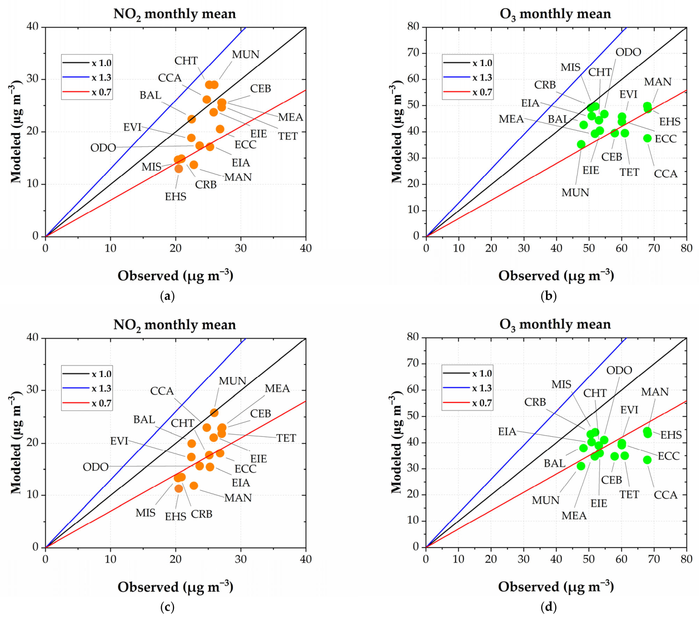
At the passive stations, the monthly mean NO2 and O3 concentrations were properly modeled in the NE 1 (81.3% and 76.5%, respectively; Figure 5a,b, Table 6). However, the performance decreased for the NE 2 (56.3% and 35.3%).
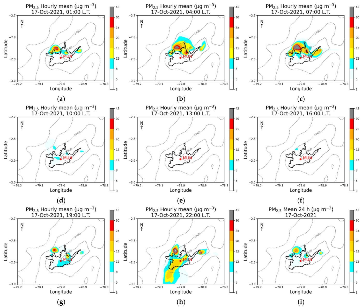
As an example of modeled air quality variables, Figure 6 illustrates the spatial distribution of the modeled hourly PM2.5 levels on 17 October 2021 for the NE 1, which ranged between 3 and 45 µg m−3. The highest levels were computed at areas north and northwest of the urban area between 04:00 and 07:00 local time (L.T.), corresponding to the influence of the emissions from artisanal brick kilns (Figure A1). The concentrations decreased with atmospheric warming during daylight hours and increased again during the night, reaching up to 20 µg m−3 at 22:00 L.T. over the urban area.
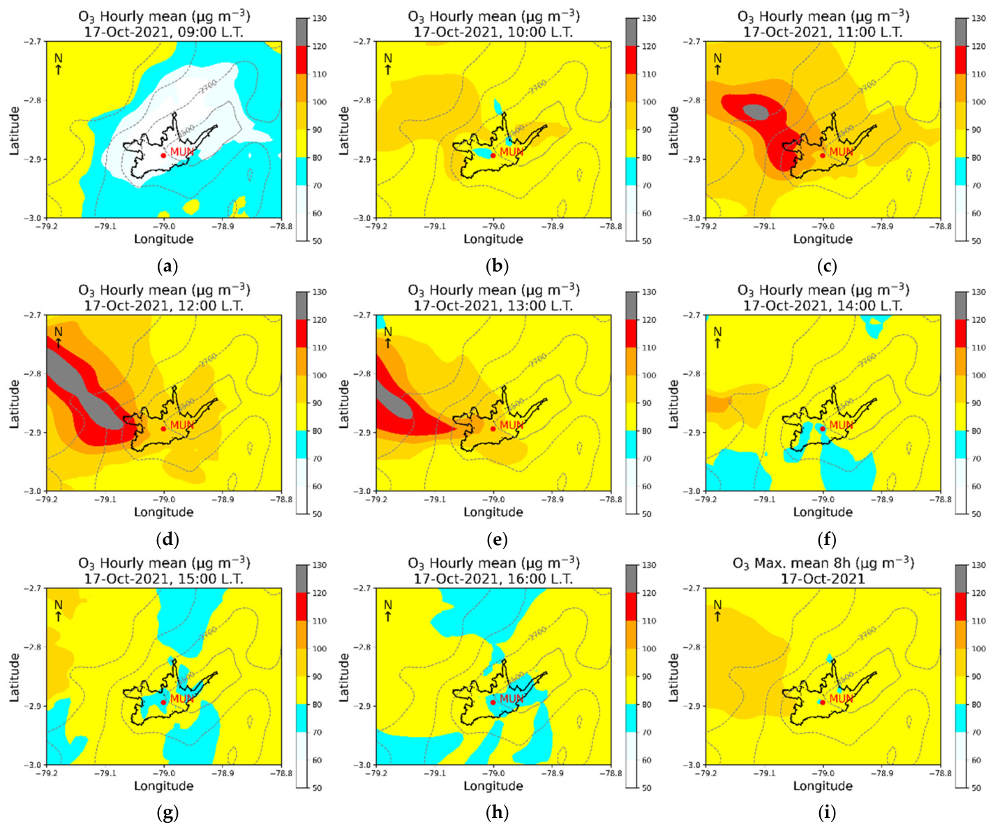
For the NE 1, Figure 7 shows the map of modeled hourly O3 levels on 17 October 2021. The highest levels were computed for the northwest and west areas outside of the urban area between 11:00 and 13:00 L.T., reaching levels of up to 130 µg m−3. At midday, the O3 levels reached 100 µg m−3 over the urban area.

3.3. Comparison to the EDGAR Emissions Dataset

Table 7 compares the EI 2021 results with the emissions for the same year from the most recent version of the EDGAR Emissions Dataset [10]. The total NOX emissions were consistent, with a ratio of 1.13 between the EI 2021 and EDGAR Dataset values. Larger differences were observed for CO and VOC emissions, with ratios of 1.72 and 2.66, respectively. The ratios for SO2 and PM2.5 emissions were 0.29 and 0.66, respectively.
The CO2 emissions were consistent, with a ratio of 1.14 between the EI 2021 value and the estimated value from the EDGAR Dataset. There were larger differences for CH4 and N2O, with ratios of 0.46 and 0.26, respectively. The ratio of total CO2-equivalent emissions was 0.93. The per capita GHG emissions were consistent, with values of 2.01 t CO2 equation per capita y−1 for the EI 2021, and 2.16 t CO2 equation per capita y−1 for the EDGAR Dataset.
For the estimation of the GHG emissions in units of CO2 equivalent, we used factors of 27 and 273 for the global warming potential of CH4 (mostly non-fossil) and N2O, respectively, which were taken from the sixth Intergovernmental Panel on Climate Change (IPCC) report [47].
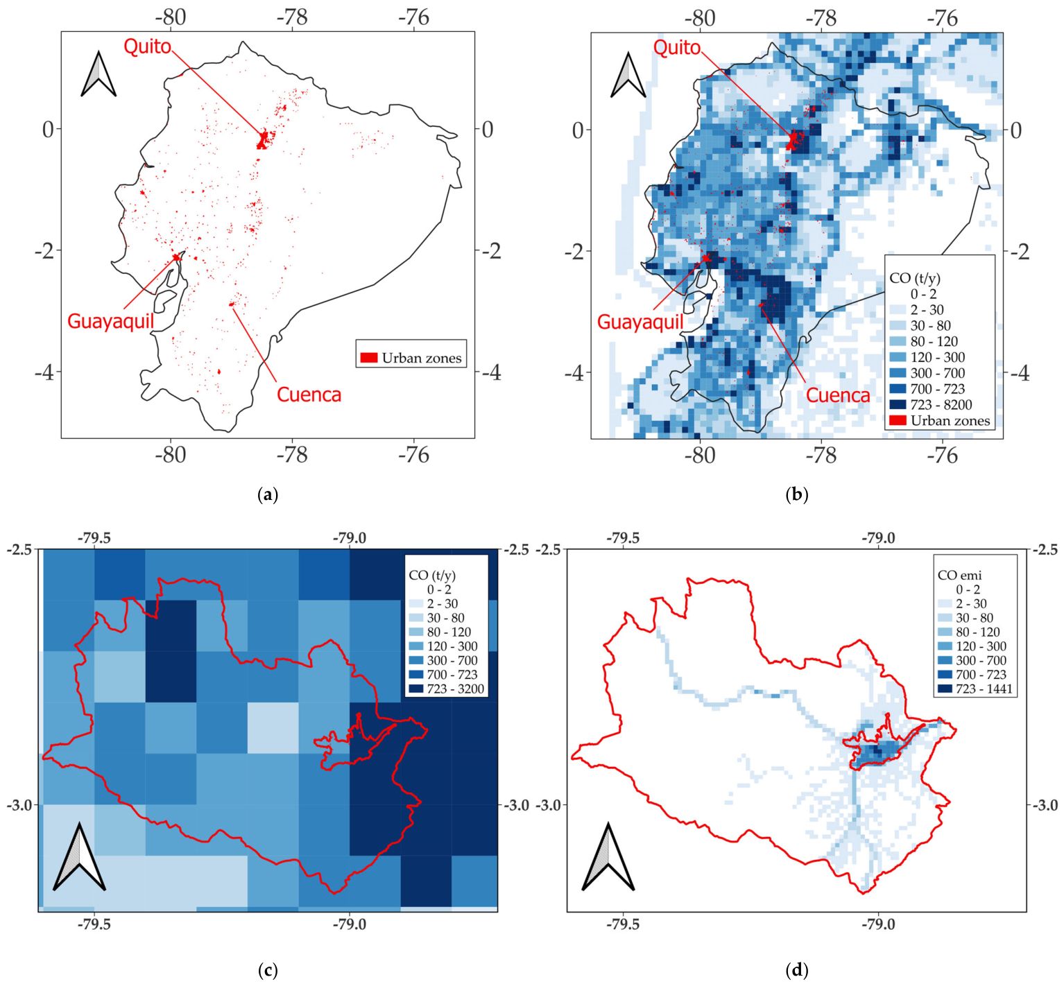
Figure 8 depicts the spatial distribution of total CO emissions. The EI 2021 map, with a 1 km spatial resolution, provides a more accurate depiction of the emissions distribution. The map generated from the EDGAR Dataset, with a resolution of approximately 11.1 km, provides a coarser resolution and even mislocalized emissions, which was also the case for the other pollutants.

4. Discussion

We assessed the quality of the EI 2021 emission inventory for Cuenca by using it as input to the WRF-Chem model to simulate atmospheric and air quality variables at a high spatial resolution (1 km). To our knowledge, this is the first time that an atmospheric emission inventory from the Equatorial Andean region has been formally assessed by modeling meteorological (surface temperature, surface wind speed, and total daily rainfall) and air pollution variables (daily mean 24 h NO2, daily mean 24 h PM2.5, daily maximum 8 h O3, and monthly mean NO2 and O3 levels). We used a state-of-the-art tool to model the direct effects of aerosols on meteorological variables and presented the results in two sets of numerical experiments, differing in boundary conditions for chemical species and in hourly profiles for disaggregating daily on-road traffic emissions.
The results and assessment depicted the current capacity of the WRF-Chem to model the atmosphere as a unique system in a complex Andean city [13,48], highlighting the variables with good, fair, and poor modeling performance. The NE 2 improved performance for the maximum 8 h O3 daily means, although it decreased long-term air quality at passive stations compared to NE 1.
The comparison of the EI 2021 results with the emissions from the EDGAR Dataset indicated a good agreement for NOx. In both cases, transportation and industry were the primary sources of NOx.
The CO emissions from the EI 2021 were 1.7 times higher than those from the EDGAR Dataset, despite the latter including additional sectors, such as agriculture. We hypothesize that the difference can be partly explained by Cuenca’s elevation (2550 masl). Molina and Molina reported that, at 2240 masl, the Mexico City Metropolitan Area has 23% less oxygen (O2) than at sea level [2]. Similarly, at the height of Cuenca, the lower O2 availability affects combustion processes, leading to higher CO emissions [49,50].
The VOC emissions from the EI 2021 were 2.7 times higher than the estimate from the EDGAR Dataset. The main reason for this difference may be that the EDGAR Dataset covers human-made sources, whereas the EI 2021, in addition to anthropogenic sources, also includes VOC emissions from vegetation.
The SO2 emissions from the EI 2021 were 0.29 times the EDGAR estimate. In both cases, industry and transportation were identified as the primary sources of SO2. Because the EMOV EP conducted a dedicated sampling campaign at service stations to characterize the sulfur content of fuels used in Cuenca in 2021, we believe that the EI 2021 estimate is more reliable.
The PM10 and PM2.5 emissions from the EI 2021 were 0.75 and 0.66 times the estimates from the EDGAR Dataset, respectively. These ratios seem consistent, as the EI 2021 did not include emissions from agricultural activities.
The comparison of the EI 2021 results with the corresponding emissions from the EDGAR Dataset indicated a good agreement for CO2. Important differences were identified for CH4 and N2O. The primary purpose of the EI 2021 was, in addition to estimating VOC emissions from vegetation, to focus on combustion and fugitive emissions from the primary human-made sources. Therefore, the EI 2021 did not include CH4 sources from enteric fermentation or agricultural or livestock activities or N2O sources from fertilizer use, all of which were included in the EDGAR Dataset.
Emission inventories are characterized by high levels of uncertainty [13]. In the case of the EI 2021, we identified components that deserve dedicated improvements in the future. In addition to the quality required for the activity data, defining emission factors for the Equatorial Andean region is a priority, considering the decrease in oxygen in the atmosphere with increasing height above sea level, which in turn increases the magnitude of emissions of primary pollutants such as CO, VOC, and particulate matter. There are very few domestic emission factors that have been characterized in Ecuador, and most of the factors studied are taken from the international literature, which has mainly focused on locations at sea level or at low elevations.
Although the modeled air quality concentrations were acceptable for most of the variables, the model’s performance can be improved. For the daily mean NO2, although the model captured the corresponding records for 84.6% of days, it yielded a low correlation coefficient. Similarly, for the daily mean PM2.5 levels, the model accurately predicted the values for 75.9% (NE 1) of days, although with a very low correlation coefficient.
As part of this research, we also used the hourly temporal profiles from the EDGAR Dataset exclusively [10] proposed for Ecuador to disaggregate the daily on-road traffic emissions. However, the modeled air quality levels notably worsened, both in magnitude and in the hourly distribution, compared to the results presented in this contribution. Therefore, a dedicated study is required to improve the estimation of hourly diesel-vehicle traffic, the most significant source of NOx and PM2.5 in the urban area of Cuenca, thereby improving the correlation coefficient of the corresponding modeled concentrations.
The RTV (Revisión Técnica Vehicular) is a technical control for the exhaust emissions and mechanical conditions of vehicles, which has been applied in Cuenca since 2008. According to national regulations, it is a prerequisite for the legal use of a vehicle throughout the year. Currently, the RTV controls hydrocarbon and carbon monoxide exhaust emissions from gasoline vehicles and opacity, a measure of how much light is blocked by particulate matter, from diesel vehicles.
The database generated by the RTV control is a valuable resource, which has been used to characterize the composition of the city’s vehicle park. This dataset includes records of the distance traveled per vehicle each year, which could enable a more accurate estimation of the on-road activity data.
There is a lack of available atmospheric records for the Andean Region of Ecuador [51,52]. Notably, the promotion of vertical sounding of meteorological and air quality species will enhance the characterization of parameters, such as the planetary boundary layer height and the vertical abundance of species, thereby providing valuable information for improving the boundary conditions used for modeling purposes and allowing for a more complete assessment of the modeling performance through the inclusion of vertical comparisons.
The EDGAR Dataset is one of the most widely used global emission resources. Georgiou et al. (2022) [7] reported the performance of an atmospheric forecasting system applied over the Eastern Mediterranean for both meteorological and air quality parameters based on the emission data from the EDGAR Dataset and WRF-Chem. Yarragunta et al. (2025) [53] utilized the EDGAR Dataset as input to WRF-Chem for atmospheric modeling, similarly assessing the performance of meteorological and air quality quantities. One advantage of the EDGAR Dataset is its consistent use of the same approach, similar to the IPCC method. However, this approach may overlook country-specific details that could enhance emission estimates and their spatial and temporal distribution [8]. The EDGAR emissions do not account for the effect of elevation on the decrease in atmospheric O2, which affects the magnitude of emissions.
Rainfall is one of the most challenging components in atmospheric modeling, especially for complex regions as the Andean region. In this contribution, we assessed the performance of rainfall modeling based on daily intensities by evaluating the model’s ability to identify days with and without rain. A more comprehensive future assessment could compare computed precipitation with records by precipitation range based on hourly intensities. For this parameter, the modeling performance was poor or fair and needs to be particularly improved.
To assess the quality of the EI 2021, we used version 3.2 of the WRF-Chem model, which had been previously tested in Cuenca to define a recommended configuration of options that we used for this study. Apart from rainfall, we identified other variables requiring better modeling performance. Global solar radiation was overestimated, which partially explains the overestimation of O3 levels in the afternoon. In the future, new versions and configurations of the WRF-Chem model can be tested to identify a set of schemes that improve the modeling of cumulus processes, thereby enhancing the representation of cloud coverage, rainfall, and surface solar radiation. Similarly, the potential benefits of indirect effects between aerosols and meteorological variables require dedicated assessments to improve atmospheric modeling in the Equatorial Andean region.
As we used the EI 2021 data within the WRF-Chem 3.2 framework, the modeling performance depends on the quality and limitations of both the EI 2021 to describe the emissions and the WRF-Chem 3.2 in modeling atmospheric variables. For air quality variables, emission data are a key input that capture the complex behavior of the atmosphere (e.g., wind speed, wind direction, planetary boundary layer height, stability dynamics).

5. Conclusions

The results indicated that most of the assessed meteorological and air quality variables were modeled acceptably across the two numerical sets (NE 1 and NE 2), suggesting that the EI 2021 emission inventory is a reasonable estimation of real emissions.
Our numerical experiments indicate that the modeling of air quality variables is sensitive to boundary conditions and to the hourly disaggregation of daily emissions. Although a complete sensitivity analysis is beyond the scope of this contribution, these two components warrant dedicated future studies.
Although October 2021 was selected to test the quality of the EI 2021, in the future, other months or even the whole annual period should be considered to account for the variability in emissions and meteorological conditions.
On the other hand, although the uncertainty of the EI 2021, it is a reasonable reference for the contributions of the most important sources of primary pollutants and GHGs in Cuenca. The EI 2021’s results can be used to explore strategies for improving air quality, such as changes in the composition of vehicle parks, the promotion of electric vehicles, improvements to fuel quality, and the use of exhaust filters in diesel vehicles. Additionally, the EI 2021 could serve as a reference for environmental impact assessments of policies, programs, and projects that affect air quality and to evaluate the performance of a preliminary atmospheric forecasting system.
To improve the atmospheric modeling, we suggest the following future research directions:
Since on-road traffic is one of the most important sources of both primary pollutants and GHGs, it is essential to maintain and update a map of daily traffic intensities on avenues, roads, and main streets. If possible, data should be collected to characterize the types and numbers of vehicles on the avenues and roads with the highest levels of traffic. For this purpose, camera-based traffic data collection should be implemented to provide additional information in order to improve the accuracy of hourly emissions estimation. Another option is to use data on the dynamic behavior of passengers’ cell phones as a proxy to infer the distribution of daily and hourly on-road traffic.
Additionally, it is necessary for each vehicle type to register the distance traveled per unit of consumed fuel. Apart from the information provided by the vehicle makers, we recommend conducting dedicated surveys of vehicle owners to obtain consistent information on the conditions in Cuenca.
Due to both short-term and long-term exceedances of the WHO guidelines [24], determining local PM2.5 emission factors is a priority, particularly for diesel vehicles and fixed sources that use fossil fuels and biomass. The RTV should also include the control of the exhaust emissions of PM2.5 and NOx from diesel cars. In fact, the RTV database of exhaust emission measurements (e.g., refs. [54,55,56]) should be used to deduce local emission factors to complement the results from the in-route use of on-board measurement devices (e.g., refs. [57,58,59]). In particular, the viability of deducing PM2.5 emission factors from opacity records deserves dedicated research, as the literature has reported conflicting correlation results (e.g., refs. [60,61]).
In addition, it is necessary to promote the definition of local emissions factors for NOx and VOC as precursors of O3. In particular, it is necessary to characterize local VOC emission factors from gasoline vehicles, vegetation, service stations, and solvents.
Regarding VOC emissions from vegetation, there are no known national or local emission factors. Additionally, there is limited information on the VOC emission capacity of some native species. Therefore, determining their emission factors [62,63] is a priority. Vegetation has high emission uncertainty. In the future, it will be necessary to characterize the spatial configuration of species and foliar biomass, as well as their dynamics throughout the year.
For future emission inventories, as a best practice, additional components can be included, such as quantification of black and elemental carbon [24].
The EI 2021 provides a coherent spatial distribution of emissions (1 km resolution), as indicated by the modeling results and performance. Apart from differences in emissions for some primary pollutants, the comparison of the geographical distribution with the EDGAR Dataset suggests that the latter would require revision to achieve performance comparable to EI 2021. For this purpose, the results from the EDGAR Dataset should be revisited to account for the effects of elevation on the magnitude and spatial distribution of primary pollutant emissions. In addition, because the EDGAR Database includes only anthropogenic sources, a vegetation VOC emission inventory is required as a relevant component for O3 modeling.
The EDGAR results could be used to calculate emissions at a high spatial resolution (1 km), potentially using proxy variables, for atmospheric modeling of cities in the equatorial Andes.
As we use EI 2021 data within the WRF-Chem 3.2 framework, modeling performance depends on both the quality and limitations of EI 2021 and the WRF-Chem 3.2 model. Emissions are the most relevant input for modeling air pollutant dynamics, and the model’s ability to describe the atmosphere modulates those dynamics. Therefore, good modeling performance is not solely attributable to inventory quality, and poor modeling performance can result not only from poor inventory but also from the model’s inability to describe atmospheric behavior. This pioneering research in the equatorial Andes area aims precisely to promote modeling with the “one atmosphere” approach, with promising results that, of course, can be improved.

Supplementary material is available from [64].

Supplementary Materials

The following supporting information can be downloaded at: https://www.mdpi.com/article/10.3390/atmos17060569/s1.

Author Contributions

Conceptualization, R.P.; methodology, R.P.; air quality and meteorological monitoring, C.C. and C.E., data curation, C.C. and C.E.; modeling, R.P.; validation, R.P., C.C. and C.E.; writing—original draft preparation, R.P.; writing—review and editing, R.P., C.C. and C.E. All authors have read and agreed to the published version of the manuscript.

Funding

This research received no external funding.

Institutional Review Board Statement

Not applicable.

Informed Consent Statement

Not applicable.

Data Availability Statement

The spatial distribution of the total yearly emissions of primary pollutants of EI 2021 (ESRI Shapefile) can be downloaded from: https://drive.google.com/file/d/1R0K5g5XA5AD29dnXlr6L0shfFcjuuS0p/view (accessed on 20 May 2026). In addition, the following data are available: the gridded yearly emissions per source; meteorological and air quality records used in this contribution to assess modeling performance are available; the coordinates of stations; the hourly percentages of daily emissions for time-disaggregated on-road traffic emissions; the namelist.wps and namelist.input files for running WRF-Chem from 1 to 3 October 2021.

Acknowledgments

This research is part of the “Emisiones atmosféricas y Calidad del Aire en el Ecuador 2026” project. Simulations were done at the High-Performance Computing system at the Universidad San Francisco de Quito.

Conflicts of Interest

The authors declare no conflicts of interest.

Abbreviations

The following abbreviations are used in this manuscript:
EDGARThe Emissions Database for Global Atmospheric Research Dataset
EI 2021The emissions inventory of Cuenca for the year 2021, assessed in this manuscript
EMOV EPEmpresa Pública Municipal de Movilidad, Tránsito y Transporte de Cuenca
ETAPA EPEmpresa Pública Municipal de Telecomunicaciones, Agua Potable, Alcantarillado y Saneamiento
GHGsGreenhouse gases
IPCCIntergovernmental Panel on Climate Change
NE 1Numerical Experiment 1
NE 2Numerical Experiment 2
RTVRevisión Técnica Vehicular
SGDsSustainable Development Goals
WHOWorld Health Organization
WRF-ChemThe Weather Research and Forecasting with Chemistry model

Appendix A

Appendix A.1. The Air Quality Network of Cuenca

The air quality network of Cuenca has been operational since 2008, in accordance with national regulations. In the city’s historic center, an automatic station (MUN, Figure 1d) measures real-time meteorological variables (temperature, wind speed, global solar radiation, and rainfall) and air quality variables (carbon monoxide, CO; sulfur dioxide, SO2; nitrogen dioxide, NO2; fine particulate matter, PM2.5; and ozone, O3). Additionally, the air quality network comprises approximately twenty passive stations distributed throughout the city to record mean monthly levels of NO2 and O3.
Records spanning more than 12 years from the MUN station indicate that PM2.5 is the pollutant of most significant concern, both in the short and long term. Typically, in September and October, O3 levels are the highest of the year, sometimes exceeding the corresponding WHO guideline value, mainly due to elevated solar radiation and, in some years, to the contribution of O3 precursor emissions from forest fires. The other pollutants (CO, NO2, SO2) were always or most of the time below the corresponding WHO guideline values.
In this way, the air quality and meteorological records from the MUN station are relevant for assessing the performance of atmospheric models in Cuenca.
Additionally, for this contribution, we collected meteorological data from two meteorological stations (SAY and SOL) located west of the urban area (Figure 1c), which are operated by ETAPA EP (Spanish acronym for Empresa Pública Municipal de Telecomunicaciones, Agua Potable, Alcantarillado y Saneamiento), the entity in charge of the water management in Cuenca. Table A1 summarizes the availability of meteorological parameters for this study.
Table A1. Meteorological stations and availability of records.
StationNomenclatureEntitymaslParameters
MunicipioMUNEMOV EP2582Temperature, wind speed, and rainfall
SayausíSAYETAPA EP2622Temperature, global solar radiation, and rainfall
SoldadosSOLETAPA EP3466Global solar radiation and rainfall

Appendix A.2. The Emission Inventory of the Year 2021 (EI 2021)

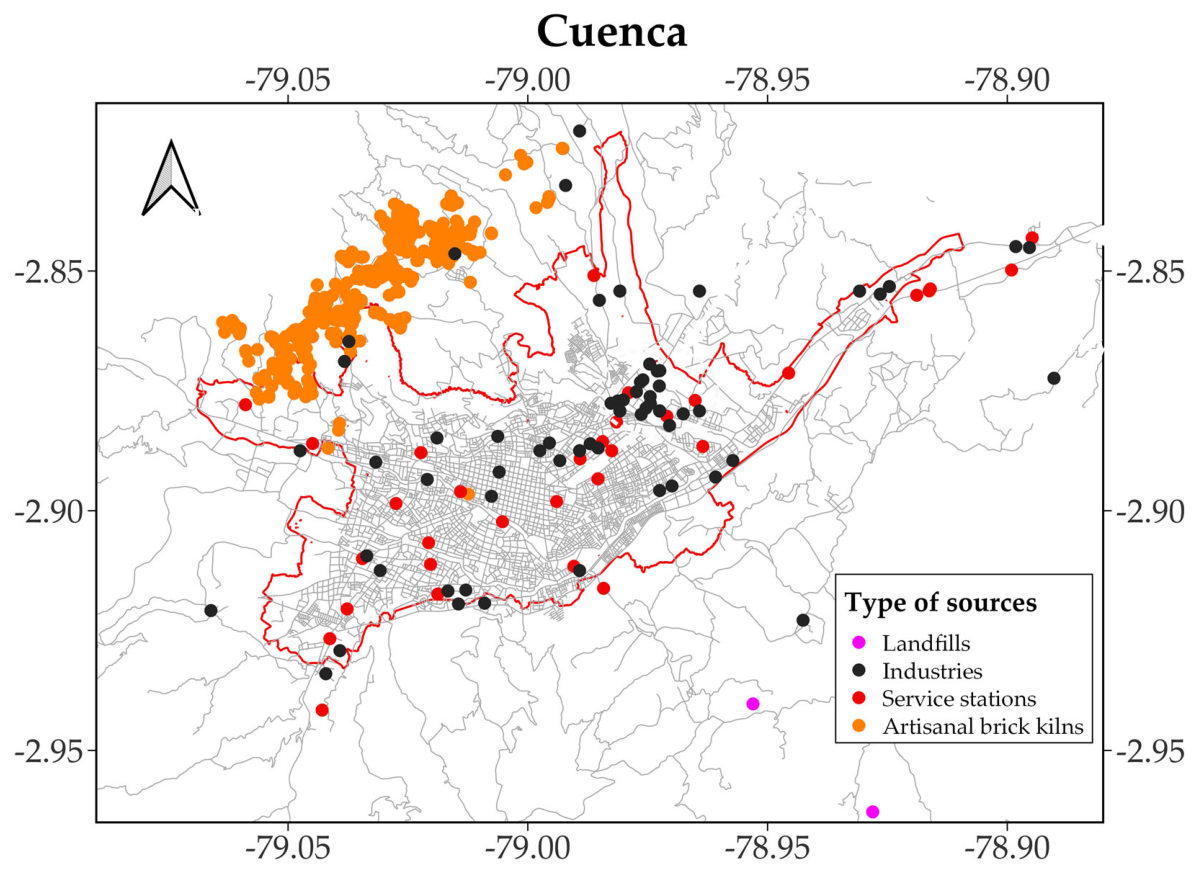
The most recent atmospheric emission inventory for Cuenca was compiled for 2021. Sources included on-road traffic, vegetation, industries, use of solvents, service stations, domestic combustion of liquid petroleum gas (LPG), air traffic, landfills, artisanal production of bricks, dust resuspension, and mining activities, under the territory of the Cantón Cuenca (Figure 1c). Figure A1 depicts the location of industries, service stations, landfills, and kilns used for the artisanal production of bricks.
The EI 2021 was developed to estimate real emissions as accurately as possible within the territory of Cuenca, with the main goals of providing a comprehensive emission inventory that can serve as a reference for air pollution management and the development of a future atmospheric forecasting system.
Figure A1. Location of selected types of emission sources.
Atmosphere 17 00569 g0a1
On-road traffic is a relevant source of emissions in Cuenca. It was estimated that about 150,800 vehicles were driven in Cuenca during 2021. Most of them (89.9%) use gasoline, while the rest (approximately 10.1%) use diesel. The presence of hybrid and electric cars was marginal. The composition of the vehicle park, in terms of percentages of used fuel, vehicle type, engine size, and year of manufacture, was deduced from statistical data of 2021 from the RTV (Spanish acronym for Revisión Técnica Vehicular), a technical control for exhaust emissions and mechanical conditions of vehicles, which has been applied in Cuenca since 2008. A survey and review of the literature were conducted to estimate the annual distances traveled and the efficiency (distance traveled per unit of fuel) by vehicle type, respectively. For consistency, the estimated fuel consumption was matched to the official statistical data on gasoline and diesel sales at Cuenca service stations for 2021. Hot, cold, and evaporative emissions were included, and the total results were spatially disaggregated on the emissions grid, using the intensity of the traffic map generated by EMOV EP as a proxy variable.
Vegetation is an important source of VOC. Apart from the type of vegetation and foliar biomass, the surface temperature and photosynthetically active radiation are the main physical drivers of VOC emissions from this source. For this purpose, meteorological data for 2021 were modeled for the emissions grid using the WRF model. Considering the temperature and photosynthetically active radiation as main physical drivers, the emissions of isoprene, monoterpenes, and other volatile organic compounds were estimated.
Combustion emissions from industries were estimated using official data on fuel consumption and emission factors from the literature.
LPG is the main fuel used in the city for domestic cooking. Similarly, the combustion emissions were estimated using official data on LPG consumption and emission factors from the literature. Total yearly emissions were spatially distributed on the grid, based on a map of population density.
The emissions of VOC from service stations were estimated using official information on the sale of fuels (gasoline and diesel) in 2021. Emissions of VOC due to the use of solvents were estimated using a per-capita emission factor and the map of population density.
Emissions from landfills were estimated using the first-order decay model proposed by the IPCC, accounting for the amount of municipal solid waste stored at each facility, the composition of the solid waste, and the landfill’s technical performance.
The yearly emissions of the primary pollutants were spatially distributed over a grid of 8000 cells (the third subdomain of the model, Figure 1c), each measuring 1 km on a side. For this purpose, the bottom-up approach was prioritized to estimate and locate the cells of emissions, complemented by the top-down approach for sources for which data are lacking and the bottom-up approach cannot be used.
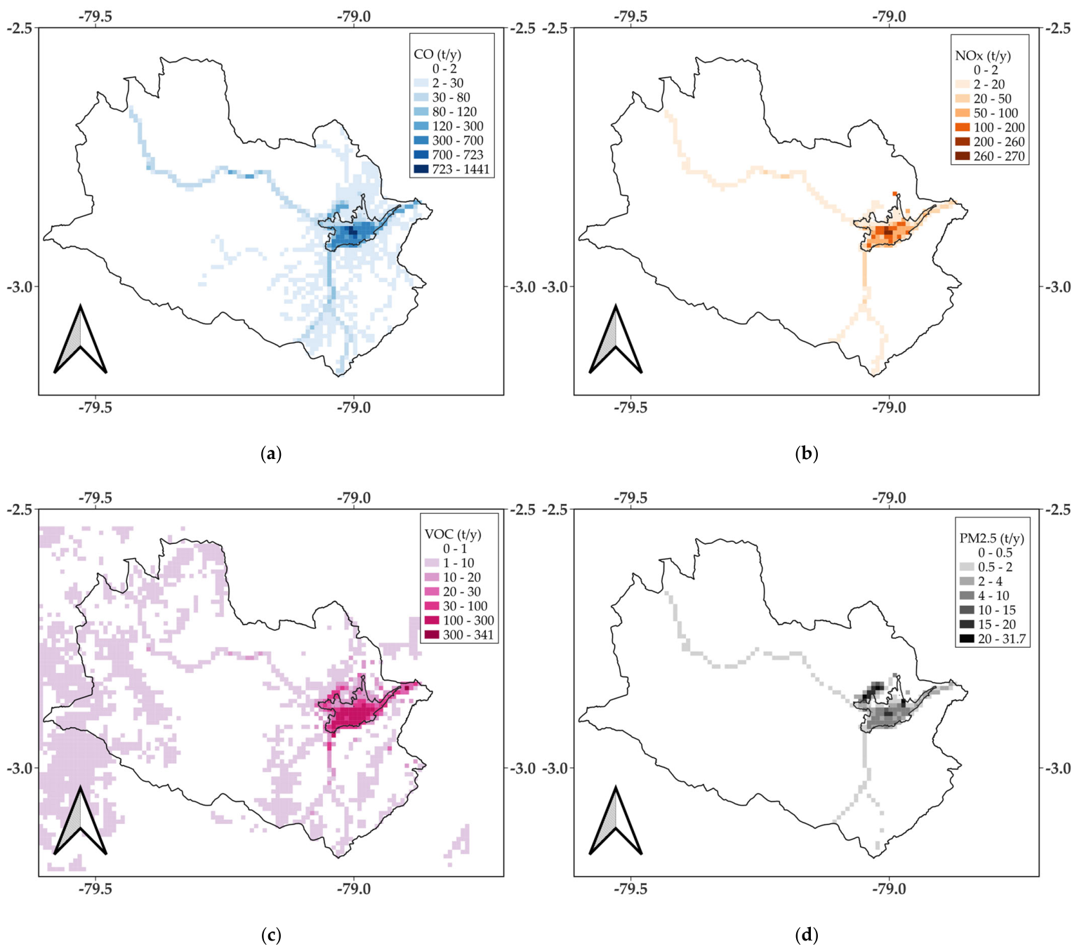
On-road traffic was the main source of NOx (89.8%), CO (95.1%), PM10 (73.3%), and PM2.5 (65%) (Table A2). Industries were the most important source of SO2 (98.0%). The use of solvents (36.0%), on-road traffic (31.8%), and vegetation (21.3%) were the main sources of VOC. After on-road traffic, artisanal bricks contributed significantly to PM10 (19.3%) and PM2.5 (27.2%) emissions. On-road traffic (66.3%), industries (20.1%), and the combustion of domestic LPG (13.0%) were the main sources of CO2 (Table A3). Figure A2 depicts the spatial distribution of the yearly emissions of CO, NOx, VOC, and PM2.5.
Table A2. Emission Inventory of Cuenca. Primary pollutants. Year 2021.
SourceNOxCOVOCSO2PM10PM2.5
t y−1%t y−1%t y−1%t y−1%t y−1%t y−1%
On-road traffic6782.489.837,624.395.14201.231.816.81.5860.173.3534.365.0
Vegetation0.00.00.00.02813.721.30.00.00.00.00.00.0
Industries555.57.4286.30.7176.51.31095.498.071.96.152.56.4
Use of solvents0.00.00.00.04752.436.00.00.00.00.00.00.0
Service stations0.00.00.00.0889.26.70.00.00.00.00.00.0
Domestic LPG162.22.125.30.15.40.00.00.010.70.910.71.3
Air traffic15.20.231.10.14.50.03.20.30.40.00.40.0
Landfills6.30.12.60.029.50.20.00.00.10.00.10.0
Artisanal bricks32.60.41577.94.0341.92.62.60.2226.219.3223.527.2
Dust resuspension0.00.00.00.00.00.00.00.00.00.00.00.0
Mining0.00.00.00.00.00.00.00.04.40.40.00.0
Total755410039,54710013,21410011181001174100822100
Table A3. Emission Inventory of Cuenca. Greenhouse gases. Year 2021.
SourceCO2CH4N2O
t y−1%t y−1%t y−1%
On-road traffic756,655.466.3203.84.183.183.3
Industries229,111.820.14.30.11.61.6
Domestic LPG148,890.413.02.30.010.210.2
Air traffic4737.20.40.20.00.20.2
Landfills2621.30.24786.695.80.00.0
Artisanal bricks53,363.70.00.20.04.74.7
Total1,142,0161004997100100100
A qualitative approach was employed to assess the uncertainty of EI 2021, using a five-category scale, ranging from A (high quality) to E (poor quality), to evaluate the quality of activity data and emission factors. Emissions by sector were classified into categories C, D, and E. The lowest grades were attributed to the quality of the emission factors.
Figure A2. Spatial distribution of the EI 2021 emissions (t y−1): (a) CO, (b) NOx, (c) VOC, (d) PM2.5.
Atmosphere 17 00569 g0a2

Appendix A.3. Data for Defining Hourly Emissions from On-Road Traffic

Figure A3. Percentages for estimating monthly on-road traffic emissions. Based on the official statistics of the monthly sales of fuels at all the service stations in Cuenca over the total amount of fuels sold in 2021.
Atmosphere 17 00569 g0a3
Figure A4. Percentages to estimate hourly on-road traffic emissions per type of day. Based on basic counting traffic data provided by the EMOV EP. Used for the Numerical Experiment 1 (NE 1).
Atmosphere 17 00569 g0a4
Figure A5. Percentages to estimate hourly on-road traffic emissions per type of day. Profile by the EMOV EP for weekdays. Profile from the EDGAR Dataset for weekends. Used for the Numerical Experiment 2 (NE 2).
Atmosphere 17 00569 g0a5

References

  1. van Aardenne, J.A. Uncertainties in Emission Inventories; Wageningen University: Wageningen, The Netherlands, 2002. [Google Scholar] [CrossRef]
  2. Molina, M.J.; Molina, L.T. Megacities and Atmospheric Pollution. J. Air Waste Manag. Assoc. 2004, 54, 644–680. [Google Scholar] [CrossRef] [PubMed]
  3. Baklanov, A.; Molina, L.T.; Gauss, M. Megacities, Air Quality and Climate. Atmos. Environ. 2016, 126, 235–249. [Google Scholar] [CrossRef]
  4. European Commission Joint Research Centre. GHG Emissions of All World Countries: 2025; European Commission Joint Research Centre: Luxembourg, 2025. [Google Scholar]
  5. Deroubaix, A.; Hoelzemann, J.J.; Ynoue, R.Y.; Toledo de Almeida Albuquerque, T.; Alves, R.C.; de Fatima Andrade, M.; Andreão, W.L.; Bouarar, I.; de Souza Fernandes Duarte, E.; Elbern, H.; et al. Intercomparison of Air Quality Models in a Megacity: Toward an Operational Ensemble Forecasting System for São Paulo. J. Geophys. Res. Atmos. 2024, 129, e2022JD038179. [Google Scholar] [CrossRef]
  6. Acdan, J.J.M.; Pierce, R.B.; Kuang, S.; McKinney, T.; Stevenson, D.; Newchurch, M.J.; Pfister, G.; Ma, S.; Tong, D. Evaluation of WRF-Chem Air Quality Forecasts during the AEROMMA and STAQS 2023 Field Campaigns. J. Air Waste Manag Assoc. 2024, 74, 783–803. [Google Scholar] [CrossRef]
  7. Georgiou, G.K.; Christoudias, T.; Proestos, Y.; Kushta, J.; Pikridas, M.; Sciare, J.; Savvides, C.; Lelieveld, J. Evaluation of WRF-Chem Model (v3.9.1.1) Real-Time Air Quality Forecasts over the Eastern Mediterranean. Geosci. Model Dev. 2022, 15, 4129–4146. [Google Scholar] [CrossRef]
  8. Matthias, V.; Arndt, J.A.; Aulinger, A.; Bieser, J.; Denier van der Gon, H.; Kranenburg, R.; Kuenen, J.; Neumann, D.; Pouliot, G.; Quante, M. Modeling Emissions for Three-Dimensional Atmospheric Chemistry Transport Models. J. Air Waste Manag. Assoc. 2018, 68, 763–800. [Google Scholar] [CrossRef]
  9. THE 17 GOALS|Sustainable Development. Available online: https://sdgs.un.org/goals (accessed on 4 May 2024).
  10. EDGAR-The Emissions Database for Global Atmospheric Research. Available online: https://EDGAR.jrc.ec.europa.eu/emissions_data_and_maps?utm_source=chatgpt.com (accessed on 7 October 2025).
  11. CAMS Global Emission Inventories. Available online: https://ads.atmosphere.copernicus.eu/datasets/cams-global-emission-inventories?tab=overview (accessed on 7 October 2025).
  12. Baklanov, A.; Zhang, Y. Advances in Air Quality Modeling and Forecasting. Glob. Transit. 2020, 2, 261–270. [Google Scholar] [CrossRef]
  13. Sokhi, R.S.; Moussiopoulos, N.; Baklanov, A.; Bartzis, J.; Coll, I.; Finardi, S.; Friedrich, R.; Geels, C.; Grönholm, T.; Halenka, T.; et al. Advances in Air Quality Research–Current and Emerging Challenges. Atmos. Chem. Phys. 2022, 22, 4615–4703. [Google Scholar] [CrossRef]
  14. Park, M.; Hu, H.; Kim, Y.; Fried, A.; Simpson, I.J.; Jin, H.; Weinheimer, A.; Huey, G.; Crawford, J.; Woo, J.-H. Evaluation of the Emission Inventory for Large Point Emission Sources in South Korea by Applying Measured Data from the NASA/NIER KORUS-AQ Aircraft Field Campaign. Elem. Sci. Anthr. 2023, 11, 00105. [Google Scholar] [CrossRef]
  15. Crippa, M.; Guizzardi, D.; Pagani, F.; Schiavina, M.; Melchiorri, M.; Pisoni, E.; Graziosi, F.; Muntean, M.; Maes, J.; Dijkstra, L.; et al. Insights into the Spatial Distribution of Global, National, and Subnational Greenhouse Gas Emissions in the Emissions Database for Global Atmospheric Research (EDGAR v8.0). Earth Syst. Sci. Data 2024, 16, 2811–2830. [Google Scholar] [CrossRef]
  16. Solazzo, E.; Crippa, M.; Guizzardi, D.; Muntean, M.; Choulga, M.; Janssens-Maenhout, G. Uncertainties in the Emissions Database for Global Atmospheric Research (EDGAR) Emission Inventory of Greenhouse Gases. Atmos. Chem. Phys. 2021, 21, 5655–5683. [Google Scholar] [CrossRef]
  17. Malasani, C.R.; Swain, B.; Patel, A.; Pulipatti, Y.; Anchan, N.L.; Sharma, A.; Vountas, M.; Liu, P.; Gunthe, S.S. Modeling of Mercury Deposition in India: Evaluating Emission Inventories and Anthropogenic Impacts. Environ. Sci. Process. Impacts 2024, 26, 1999–2009. [Google Scholar] [CrossRef] [PubMed]
  18. Baklanov, A.; Brunner, D.; Carmichael, G.; Flemming, J.; Freitas, S.; Gauss, M.; Hov, Ø.; Mathur, R.; Schlünzen, K.H.; Seigneur, C.; et al. Key Issues for Seamless Integrated Chemistry–Meteorology Modeling. Bull. Am. Meteorol. Soc. 2017, 98, 2285–2292. [Google Scholar] [CrossRef] [PubMed]
  19. Parra, R. Inventario de Emisiones Atmosféricas Del Cantón Cuenca 2014; Empresa Pública de Movilidad, Tránsito y Transporte (EMOV EP): Cuenca, Ecuador, 2016. [Google Scholar] [CrossRef]
  20. Parra, R. Assessment of Land Surface Schemes from the WRF-Chem for Atmospheric Modeling in the Andean Region of Ecuador. Atmosphere 2023, 14, 508. [Google Scholar] [CrossRef]
  21. Parra, R. Impact of Cumulus Options from Weather Research and Forecasting with Chemistry in Atmospheric Modeling in the Andean Region of Southern Ecuador. Atmosphere 2024, 15, 693. [Google Scholar] [CrossRef]
  22. EMOV. Available online: https://caire.emov.gob.ec/ (accessed on 22 February 2025).
  23. EMOV. Available online: https://caire.emov.gob.ec/informes (accessed on 22 February 2025).
  24. World Health Organization. WHO Global Air Quality Guidelines: Particulate Matter (PM2.5 and PM10), Ozone, Nitrogen Dioxide, Sulfur Dioxide and Carbon Monoxide; World Health Organization: Geneva, Switzerland, 2021. [Google Scholar]
  25. Parra, R.; Molina, C.; Caguana, C.; Heredia, E. Inventario de Emisiones Atmosféricas Del Cantón Cuenca 2021; Empresa Pública de Movilidad, Tránsito y Transporte (EMOV EP): Cuenca, Ecuador, 2023. [Google Scholar]
  26. EMEP/EEA Air Pollutant Emission Inventory Guidebook 2023. Available online: https://www.eea.europa.eu/en/analysis/publications/emep-eea-guidebook-2023 (accessed on 13 February 2025).
  27. Guenther, A.B.; Zimmerman, P.R.; Harley, P.C.; Monson, R.K.; Fall, R. Isoprene and Monoterpene Emission Rate Variability: Model Evaluations and Sensitivity Analyses. J. Geophys. Res. Atmos. 1993, 98, 12609–12617. [Google Scholar] [CrossRef]
  28. Guenther, A.; Hewitt, C.N.; Erickson, D.; Fall, R.; Geron, C.; Graedel, T.; Harley, P.; Klinger, L.; Lerdau, M.; Mckay, W.A.; et al. A Global Model of Natural Volatile Organic Compound Emissions. J. Geophys. Res. Atmos. 1995, 100, 8873–8892. [Google Scholar] [CrossRef]
  29. TFI—IPCC. Available online: https://www.ipcc.ch/working-group/tfi/ (accessed on 8 February 2025).
  30. Skamarock, W.C.; Klemp, J.B.; Dudhia, J.; Gill, D.O.; Barker, D.M.; Duda, M.G.; Huang, X.-Y.; Wang, W.; Powers, J.G. A Description of the Advanced Research WRF Version 3; National Center for Atmospheric Research: Boulder, CO, USA, 2008. [Google Scholar]
  31. CISL RDA: NCEP FNL Operational Model Global Tropospheric Analyses, Continuing from July 1999. Available online: https://rda.ucar.edu/datasets/ds083.2/ (accessed on 30 December 2022).
  32. Zaveri, R.A.; Peters, L.K. A New Lumped Structure Photochemical Mechanism for Large-Scale Applications. J. Geophys. Res. 1999, 104, 30387–30415. [Google Scholar] [CrossRef]
  33. Zaveri, R.A.; Easter, R.C.; Fast, J.D.; Peters, L.K. Model for Simulating Aerosol Interactions and Chemistry (MOSAIC). J. Geophys. Res. 2008, 113, D13204. [Google Scholar] [CrossRef]
  34. Espinoza Molina, C.; Claudia, C. Informe de Calidad Del Aire Cuenca 2021; EMOV EP: Cuenca, Ecuador, 2022; Available online: https://www.researchgate.net/publication/362194795_Informe_de_Calidad_del_Aire_Cuenca_2021 (accessed on 20 May 2026).
  35. Hong, S.-Y.; Dudhia, J.; Chen, S.-H. A Revised Approach to Ice Microphysical Processes for the Bulk Parameterization of Clouds and Precipitation. Mon. Wea. Rev. 2004, 132, 103–120. [Google Scholar] [CrossRef]
  36. Mlawer, E.J.; Taubman, S.J.; Brown, P.D.; Iacono, M.J.; Clough, S.A. Radiative Transfer for Inhomogeneous Atmospheres: RRTM, a Validated Correlated-k Model for the Longwave. J. Geophys. Res. 1997, 102, 16663–16682. [Google Scholar] [CrossRef]
  37. Chou, M.-D.; Suarez, M.J. A Solar Radiation Parameterization for Atmospheric Studies; NASA/TM-1999-104606/VOL15. 1999. Available online: https://ntrs.nasa.gov/citations/19990060930 (accessed on 30 December 2022).
  38. Paulson, C.A. The Mathematical Representation of Wind Speed and Temperature Profiles in the Unstable Atmospheric Surface Layer. J. Appl. Meteor. 1970, 9, 857–861. [Google Scholar] [CrossRef]
  39. Hong, S.-Y.; Noh, Y.; Dudhia, J. A New Vertical Diffusion Package with an Explicit Treatment of Entrainment Processes. Mon. Weather Rev. 2006, 134, 2318–2341. [Google Scholar] [CrossRef]
  40. Chen, F.; Dudhia, J. Coupling an Advanced Land Surface–Hydrology Model with the Penn State–NCAR MM5 Modeling System. Part II: Preliminary Model Validation. Mon. Wea. Rev. 2001, 129, 587–604. [Google Scholar] [CrossRef]
  41. The Application of Models Under the European Union’s Air Quality Directive: A Technical Reference Guide—European Environment Agency. Available online: https://www.eea.europa.eu/publications/fairmode (accessed on 30 December 2022).
  42. Rain Day-Glossary of Meteorology. Available online: https://glossary.ametsoc.org/wiki/rain-day (accessed on 20 May 2026).
  43. Acuerdo No 97/A-Norma de Calidad del Aire Ambiente o Nivel de Inmisión (Anexo 4, Libro VI de la Calidad Ambiental, del Texto Unificado de la Legislación Secundaria del Ministerio del Ambiente).|FAOLEX. Available online: https://www.fao.org/faolex/results/details/es/c/LEX-FAOC155133/ (accessed on 25 July 2024).
  44. World Health Organization (Ed.) Air Quality Guidelines: Global Update 2005: Particulate Matter, Ozone, Nitrogen Dioxide, and Sulfur Dioxide; World Health Organization: Copenhagen, Denmark, 2006. [Google Scholar]
  45. Simon, H.; Baker, K.R.; Phillips, S. Compilation and Interpretation of Photochemical Model Performance Statistics Published between 2006 and 2012. Atmos. Environ. 2012, 61, 124–139. [Google Scholar] [CrossRef]
  46. Crippa, M.; Solazzo, E.; Huang, G.; Guizzardi, D.; Koffi, E.; Muntean, M.; Schieberle, C.; Friedrich, R.; Janssens-Maenhout, G. High Resolution Temporal Profiles in the Emissions Database for Global Atmospheric Research. Sci. Data 2020, 7, 121. [Google Scholar] [CrossRef]
  47. Intergovernmental Panel on Climate Change (IPCC). Climate Change 2021—The Physical Science Basis: Working Group I Contribution to the Sixth Assessment Report of the Intergovernmental Panel on Climate Change, 1st ed.; Cambridge University Press: Cambridge, UK, 2023. [Google Scholar] [CrossRef]
  48. Gao, Z.; Zhou, X. A Review of the CAMx, CMAQ, WRF-Chem and NAQPMS Models: Application, Evaluation and Uncertainty Factors. Environ. Pollut. 2024, 343, 123183. [Google Scholar] [CrossRef]
  49. Qi, Z.; Gu, M.; Cao, J.; Zhang, Z.; You, C.; Zhan, Y.; Ma, Z.; Huang, W. The Effects of Varying Altitudes on the Rates of Emissions from Diesel and Gasoline Vehicles Using a Portable Emission Measurement System. Atmosphere 2023, 14, 1739. [Google Scholar] [CrossRef]
  50. Jiang, Z.; Wu, L.; Niu, H.; Jia, Z.; Qi, Z.; Liu, Y.; Zhang, Q.; Wang, T.; Peng, J.; Mao, H. Investigating the Impact of High-Altitude on Vehicle Carbon Emissions: A Comprehensive on-Road Driving Study. Sci. Total Environ. 2024, 918, 170671. [Google Scholar] [CrossRef]
  51. Cazorla, M.; Parra, R.; Herrera, E.; da Silva, F.R. Characterizing Ozone throughout the Atmospheric Column over the Tropical Andes from in Situ and Remote Sensing Observations. Elem. Sci. Anthr. 2021, 9, 00019. [Google Scholar] [CrossRef]
  52. Campozano, L.; Célleri, R.; Trachte, K.; Bendix, J.; Samaniego, E. Rainfall and Cloud Dynamics in the Andes: A Southern Ecuador Case Study. Adv. Meteorol. 2016, 2016, 3192765. [Google Scholar] [CrossRef]
  53. Yarragunta, Y.; Francis, D.; Fonseca, R.; Nelli, N. Evaluation of the WRF-Chem Performance for the Air Pollutants over the United Arab Emirates. Atmos. Chem. Phys. 2025, 25, 1685–1709. [Google Scholar] [CrossRef]
  54. Jaworski, A.; Kuszewski, H.; Ustrzycki, A.; Balawender, K.; Lejda, K.; Woś, P. Analysis of the Repeatability of the Exhaust Pollutants Emission Research Results for Cold and Hot Starts under Controlled Driving Cycle Conditions. Environ. Sci. Pollut. Res. 2018, 25, 17862–17877. [Google Scholar] [CrossRef]
  55. Valverde, V.; Mora, B.A.; Clairotte, M.; Pavlovic, J.; Suarez-Bertoa, R.; Giechaskiel, B.; Astorga-LLorens, C.; Fontaras, G. Emission Factors Derived from 13 Euro 6b Light-Duty Vehicles Based on Laboratory and On-Road Measurements. Atmosphere 2019, 10, 243. [Google Scholar] [CrossRef]
  56. Park, G.; Mun, S.; Hong, H.; Chung, T.; Jung, S.; Kim, S.; Seo, S.; Kim, J.; Lee, J.; Kim, K.; et al. Characterization of Emission Factors Concerning Gasoline, LPG, and Diesel Vehicles via Transient Chassis-Dynamometer Tests. Appl. Sci. 2019, 9, 1573. [Google Scholar] [CrossRef]
  57. Kousoulidou, M.; Fontaras, G.; Ntziachristos, L.; Bonnel, P.; Samaras, Z.; Dilara, P. Use of Portable Emissions Measurement System (PEMS) for the Development and Validation of Passenger Car Emission Factors. Atmos. Environ. 2013, 64, 329–338. [Google Scholar] [CrossRef]
  58. Rivera-Campoverde, N.D.; Muñoz-Sanz, J.L.; Arenas-Ramirez, B.d.V. Estimation of Pollutant Emissions in Real Driving Conditions Based on Data from OBD and Machine Learning. Sensors 2021, 21, 6344. [Google Scholar] [CrossRef] [PubMed]
  59. Perdikopoulos, M.; Karageorgiou, T.; Ntziachristos, L.; Deville Cavellin, L.; Joly, F.; Vigneron, J.; Arfire, A.; Debert, C.; Sanchez, O.; Gaie-Levrel, F.; et al. Developing Emission Factors from Real-World Emissions of Euro VI Urban Diesel, Diesel-Hybrid, and Compressed Natural Gas Buses. Atmosphere 2025, 16, 293. [Google Scholar] [CrossRef]
  60. Clark, N.N.; Gautam, M. Evaluation of Technology to Support a Heavy-Duty Diesel Vehicle Inspection and Maintenance Program; West Virginia University: Morgantown, WV, USA, 2001. [Google Scholar]
  61. Yang, H.-H.; Kumar, A.; Dhital, N.B.; Wang, L.-C.; Wu, C.-H.; Kamyab, H.; Yusuf, M. Evaluating the Feasibility of Estimating Particulate Mass Emissions of Older-Model Diesel Vehicle Using Smoke Opacity Measurements. Sci. Rep. 2024, 14, 31494. [Google Scholar] [CrossRef] [PubMed]
  62. Bracho-Nunez, A.; Welter, S.; Staudt, M.; Kesselmeier, J. Plant-Specific Volatile Organic Compound Emission Rates from Young and Mature Leaves of Mediterranean Vegetation. J. Geophys. Res. Atmos. 2011, 116, D16. [Google Scholar] [CrossRef]
  63. Laguerre, A.; Brennan, D.L.; Starry, O.; Rosenstiel, T.N.; Gall, E.T. Characterization of Volatile Organic Compound Emissions and CO2 Uptake from Eco-Roof Plants. Build. Environ. 2023, 234, 110158. [Google Scholar] [CrossRef] [PubMed]
  64. EMOV. Available online: https://drive.google.com/file/d/1R0K5g5XA5AD29dnXlr6L0shfFcjuuS0p/view (accessed on 20 May 2026).
Figure 1. (a) Location of Ecuador. (b,c) Location of the Cantón Cuenca and meteorological stations (white dots). (c) The black rectangle indicates the border of the third subdomain for modeling, a grid composed of 100 columns and 80 rows. (d) Urban area of Cuenca (red border) and the stations of the air quality network (red dots). MUN is an automatic station for both meteorological and air quality variables. The remaining sixteen red dots indicate the locations of passive stations that were considered for this manuscript.
Atmosphere 17 00569 g001
Figure 2. Daily mean profiles during October 2021: (a) MUN station: surface temperature. (b) MUN station: wind speed. (c) SOL station: global solar radiation.
Atmosphere 17 00569 g002
Figure 3. Numerical Experiment 1 (NE 1): rainfall records (observed) and modeled values (mm d−1). (a) MUN station. (b) SAY station. (c) SOL station.
Atmosphere 17 00569 g003
Figure 4. Observed versus modeled daily concentrations: (a) NO2 24 h mean; (b) mean daily profiles of hourly NO2; (c) PM2.5 24 h mean; (d) mean daily profiles of hourly PM2.5; (e) O3 8 h maximum; (f) mean daily profiles of hourly O3.
Atmosphere 17 00569 g004
Figure 5. Observed versus modeled levels at passive stations: Numerical Experiment 1 (NE 1): (a) NO2 and (b) O3. Numerical Experiment 2 (NE 2): (c) NO2 and (d) O3.
Atmosphere 17 00569 g005
Figure 6. Numerical Experiment 1 (NE 1): Modeled PM2.5 levels for 17 October 2021. Results in local time (L.T.). Hourly mean concentrations: (a) 01:00, (b) 04:00, (c) 07:00, (d) 10:00, (e) 13:00, (f) 16:00, (g) 19:00, (h) 22:00. (i) Mean concentration during 24 h.
Atmosphere 17 00569 g006
Figure 7. Numerical Experiment 1 (NE 1): Modeled O3 levels for 17 October 2021. Results in local time (L.T.). Hourly mean concentrations: (a) 09:00, (b) 10:00, (c) 11:00, (d) 12:00, (e) 13:00, (f) 14:00, (g) 15:00, (h) 16:00. (i) Maximum mean concentration during 8 h.
Atmosphere 17 00569 g007
Figure 8. Spatial distribution of the CO emission for the year 2021: (a) Ecuador, main urban zone. (b) Ecuador, EDGAR Dataset (spatial resolution: 11.1 km). (c) Cuenca, EDGAR Dataset (spatial resolution 11.1 km). (d) Cuenca, EI 2021 (spatial resolution: 1 km).
Atmosphere 17 00569 g008
Table 3. Metrics for modeling meteorological variables. Bold numbers are in the benchmark.
MetricMUNSAYBenchmark
Hourly surface temperature:
NE 1NE 2NE 1NE 2
GE1.461.542.112.18<2 °C
MB0.610.490.740.62(−0.5 °C, 0.5 °C)
IOA0.840.830.860.85≥0.8
Hourly wind speed:
NE 1NE 2NE 1NE 2
RMSE1.041.08NANA<2 m s−1
MB0.310.36NANA(−0.5 m s−1, 0.5 m s−1)
IOA0.720.71NANA≥0.6
NA: Not assessed.
Table 4. Percentage of records captured by modeling meteorological variables.
ParameterMUNSAYSOL
NE 1NE 2NE 1NE 2NE 1NE 2
Hourly surface temperature78.477.460.358.9NANA
Hourly wind speed75.876.1NANANANA
Daily rainfall46.755.780.073.373.366.7
NA: Not assessed.
Table 5. Short-term air quality metrics.
NE 1NE 2Ideal ValueNumber of Assessed Days (Total = 30 Days)Percentage of Days for Assessing
24 h NO2 mean:
MB1.1−2.202686.7
RMSE10.39.602686.7
r0.10.212686.7
24 h PM2.5 mean:
MB−3.52−3.7602996.7
RMSE5.425.6702996.7
r−0.11−0.0912996.7
Maximum 8 h O3 mean:
MB10.702.9002893.3
RMSE17.0016.9002893.3
r0.600.112893.3
Table 6. Percentage of records captured by modeling air quality variables.
NE 1NE 2
Short-term air quality:
24 h NO2 mean84.684.6
24 h PM2.5 mean75.972.4
Max. 8 h O3 mean67.982.1
Average:76.179.7
Long-term air quality:
NO2, monthly mean81.356.3
O3, monthly mean76.535.3
Average:78.945.8
Table 7. Comparison to the results from the EDGAR Emissions Dataset. Year 2021.
This ContributionEDGAR DatasetDifference
Primary pollutants(t/y)(t/y)(%)
NOx75546690−11.4
CO39,54722,986−41.9
VOC13,2144970−62.4
SO211183851244.5
PM101174155832.7
PM2.5822123750.4
Greenhouse gases(t/y)(t/y)(%)
CO21,142,0161,004,333−12.1
CH4499710,815116.4
N2O100392291.9
Total greenhouse gases(t CO2 equation/y)(t CO2 equation/y)(%)
CO2 equation1,304,2351,403,3327.6
Greenhouse gases emissions per capita:(t CO2 equation per capita/y)(t CO2 equation per capita/y)(%)
CO2 equation per capita2.012.167.6
Disclaimer/Publisher’s Note: The statements, opinions and data contained in all publications are solely those of the individual author(s) and contributor(s) and not of MDPI and/or the editor(s). MDPI and/or the editor(s) disclaim responsibility for any injury to people or property resulting from any ideas, methods, instructions or products referred to in the content.