Article

Spatial Decoupling of Surface and Atmospheric Urban Heat: Differential Land Cover Associations in Zagreb


1
Department of Geography, Faculty of Science, University of Zagreb, 10000 Zagreb, Croatia
2
Chair of Photogrammetry and Remote Sensing, Faculty of Geodesy, University of Zagreb, 10000 Zagreb, Croatia
*
Author to whom correspondence should be addressed.
Atmosphere 2026, 17(5), 466; https://doi.org/10.3390/atmos17050466
Submission received: 31 March 2026 / Revised: 24 April 2026 / Accepted: 27 April 2026 / Published: 30 April 2026
(This article belongs to the Special Issue Urban Impact on the Low Atmosphere Processes)

Abstract

Urban heat islands present a significant obstacle to climate adaptation strategies, yet the interplay between surface and atmospheric thermal elements is not fully understood. This research investigates the spatial relationship between land surface temperature (LST) and near-surface air temperature (TAIR) across Zagreb’s 218 local councils during the summer of 2024, assessing the premise that these constitute separate thermal dimensions with varying land cover correlations. Landsat 8/9-derived LST and CERRA-derived TAIR, temporally aligned to the Landsat overpass slot (09:00 UTC), were examined through spatial autocorrelation (Moran’s I, Getis–Ord Gi*), correlation analysis, and Fisher’s z-tests to compare the effects of the Normalized Difference Vegetation Index (NDVI) and Normalized Difference Built-up Index (NDBI). The findings indicated partial coupling (r = 0.537, R2 = 0.288), with 71.2% of the variance remaining unexplained, suggesting considerable surface-atmospheric decoupling. Furthermore, hot spot overlap analysis revealed limited convergence (11.9% of neighborhoods), while 44.5% displayed divergent thermal extremes. Land cover showed much stronger connections with LST (NDVI: r = −0.970, R2 = 0.941; NDBI: r = +0.973, R2 = 0.947) than with TAIR (NDVI: r = −0.478; NDBI: r = +0.496), representing reductions in explained variance of 63–64% (p < 0.001). These findings suggest that surface and atmospheric urban heat are related but distinct thermal aspects.

1. Introduction

1.1. LST vs. TAIR: Conceptual Distinction and Methodological Implications

Urban thermal environments are conventionally characterized through two distinct yet related measures: land surface temperature (LST), representing the radiative temperature of the Earth’s surface as captured by satellite sensors, and near-surface air temperature (TAIR), typically measured or estimated at 1–2 m above ground level where human thermal exposure occurs. While both metrics are frequently employed to define urban heat islands, they fundamentally measure different components of the urban thermal regime: surface radiative properties versus atmospheric thermal conditions with potentially divergent spatial patterns and driving mechanisms.
Land surface temperature (LST) and near-surface air temperature (TAIR) represent different, though related, components of the urban thermal environment; LST measures the radiative temperature of the Earth’s surface, while TAIR indicates the temperature at a height of 1–2 m above the ground [1]. These two variables demonstrate differing spatiotemporal properties, with LST typically exhibiting greater diurnal variability than TAIR [2,3]. Recent studies employing crowdsourced air temperature data in European cities have shown that the intensity of the urban heat island effect can be overestimated by 1.19 ± 0.02 °C when LST is used instead of TAIR, which equates to a sixfold overestimation [4]. The disparity between land surface temperature (LST) and air temperature (TAIR) fluctuates based on diurnal patterns, seasonal shifts, and land cover types, with the most pronounced differences occurring during the summer months and in the early afternoon [2,3]. LST demonstrates significantly greater spatial variability within urban areas compared to TAIR, particularly during the warmer seasons; moreover, more substantial differences are evident within built environments when contrasted with natural local climate zones [5]. This dynamic is further modulated by meteorological conditions, including cloud cover and wind speed [2,3]. For instance, in Madison, Wisconsin, the least significant heat island effect was recorded in daytime air temperature, where the disparity between the maximum and minimum pixel values was a mere 1.22 °C; in contrast, the land surface temperature (LST) anomaly exhibited the widest range, extending from −15.44 °C to 3.97 °C [6]. The correlation between the day of the year and the LST-TAIR relationship was successfully represented by a parabolic curve (R2 = 0.76, p = 0.0002), peaking in late July, which implies that plant phenology affects these seasonal variations [6]. Furthermore, within urban areas marked by heterogeneity, the spatial arrangement of TAIR hot spots does not uniformly correspond with LST, thereby indicating the existence of unique thermal patterns [5]. Consequently, statistical and machine learning models have been formulated to estimate TAIR using LST and supplementary predictors. Random Forest models, which incorporate MODIS LST, ERA5-Land meteorological variables, and local climate zone data, have demonstrated daytime and nighttime RMSE values nearing 0.5 °C [7]. Furthermore, sophisticated downscaling methodologies that merge LST with NDVI, NDBI, NDWI, elevation, and urban morphology parameters exhibit enhanced efficacy when contrasted with conventional thermal sharpening techniques [8,9]. Machine learning methodologies, including Random Forest, Support Vector Regression, and Extreme Gradient Boosting, have attained R2 values reaching 0.82 within semi-arid settings [10]. In addition, the integration of Shapley Additive Explanations (SHAP) has improved interpretability, thereby identifying normalized difference indices as the most influential predictors [11]. Deep learning super-resolution methods have shown success in converting coarse 0.25° forecasts into 1 km air temperature fields, which has led to a more than 20% decrease in 7-day forecast errors [12]. In addition, using Sentinel-2 spectral indices allows for the downscaling of Landsat-derived land surface temperature (LST) data from a 30 m resolution to a 10 m resolution, achieved through the use of multiple linear regression models [13].

1.2. Land Cover Effects on Urban Thermal Environments

Urban vegetation reduces temperatures through evapotranspiration, shading, and albedo modification [14,15]. Reviews suggest vegetation cooling can lower urban temperatures by 0.5 to 4.0 °C, with green roofs producing surface cooling effects of up to 60 °C [15,16]. Mesoscale modeling studies have recently shown that the cooling effects of vegetation display distinct daily patterns, with varying responses to extreme heat. Evapotranspiration-driven cooling strengthens after sunrise, reaching its maximum in the late morning before a rapid decrease, whereas shading-based cooling gradually increases before noon but may transition to heat retention during the night [17]. During periods of extreme heat, an elevated vapor pressure deficit causes evapotranspiration cooling to peak earlier and to a greater extent, followed by a more pronounced decline due to physiological limitations. Furthermore, vegetation cooling is influenced by canopy structure, leaf area index, vegetation height, and the presence of adjacent impervious surfaces, with meteorological conditions primarily dictating diurnal fluctuations [17,18]. NDVI has been identified as primary indicator of urban heat mitigation through evapotranspiration [18]. The Normalized Difference Vegetation Index (NDVI) serves as an indicator of vegetation health and density well-suited for modeling urban thermal environments [19]. Studies consistently demonstrate negative NDVI-LST correlations, with areas exhibiting higher vegetation experiencing lower temperatures [20,21]. Research in island cities confirms NDVI represents the main factor for reducing urban LST, especially during summer [22]. Ground observations found daytime temperatures 3 to 6 °C cooler underneath tall canopy compared to bare ground [23]. The relationship between NDVI and LST displays both seasonal fluctuations and non-linear properties. Within Beijing’s Olympic Area, NDVI was the primary influencing factor, accounting for 40% of the variance in summer, 21% in autumn, and 19% in winter [24]. The degree of influence is contingent upon urban morphological types; vegetation demonstrates a strong explanatory power in open, low-rise blocks, whereas its significance diminishes in high-density areas [25]. Vegetation’s spatial arrangement significantly influences temperature patterns, a process governed by complex interactions with built structures that modify shared radiation and thermal environments [26]. The dimensions of urban green spaces are also critical; larger areas, especially those incorporating urban forests, contribute to the formation of distinctive microclimates [27]. The Normalized Difference Built-up Index (NDBI), which quantifies built-up density, exhibits consistent positive correlations with land surface temperature (LST) [28]. Research indicates that NDBI is the most significant factor contributing to warming, particularly during the spring, with a contribution rate of 45.5% [24,29]. Urban built-up areas and impervious surfaces substantially increase LST due to their low albedo, elevated heat capacity, and minimal evapotranspiration [25,30]. Three-dimensional (3D) urban morphology exhibits non-linear influences on land surface temperature (LST). Building height and density exert a dual influence: they impede heat dissipation through heat retention, while also providing shade [25,31]. Within a constant block density, a higher average height is associated with a lower LST [22]. The Sky View Factor (SVF) is recognized as the most influential cooling factor among the 3D metrics [24,31]. The relative importance of 2D versus 3D factors varies seasonally; specifically, 2D land-use variables demonstrate the strongest correlations during summer and spring, whereas 3D building variables exert a more substantial influence during the colder months [24,32]. Furthermore, building density and height together account for over 75% of the LST variance across all four seasons [32]. In urban environments, NDVI and NDBI frequently exhibit significant collinearity, with correlation coefficients approaching r ≈ −0.99 [33]. This almost perfect inverse correlation suggests that these indices represent a singular underlying land cover dimension, specifically a vegetated-to-built-up gradient, rather than independent influences [34]. Consequently, when incorporated simultaneously into regression models, such collinearity produces variance inflation factors surpassing 50, which in turn leads to unstable coefficients [34]. To mitigate this issue, researchers frequently employ separate modeling strategies, analyzing NDVI and NDBI independently [35]. Furthermore, alternative methodologies involve composite indices that integrate both metrics to differentiate between permeable and impervious surfaces [17].

1.3. Spatial Autocorrelation in Urban Thermal Analysis

Spatial autocorrelation represents correlation of variable with itself in geographical space, observable at all spatial scales [36]. In urban thermal analysis, Moran’s I is the main way to measure global spatial autocorrelation. It helps determine if temperature patterns are clustered, spread out, or random [37]. High positive Moran’s I values indicate LST values are more spatially clustered than expected under random processes [38,39]. Local indicators of spatial association (LISA), such as Local Moran’s I and Getis–Ord Gi*, are utilized to pinpoint specific locations of clusters and spatial outliers [40,41]. The Getis–Ord Gi* statistic is especially useful for identifying hot spots (high-value clusters) and cold spots (low-value clusters); positive and statistically significant values suggest the presence of heat island formation [39,42]. Unlike Local Moran’s I, the Getis–Ord method does not consider spatial outliers, focusing exclusively on identifying clusters [40]. Studies utilizing spatial autocorrelation within urban thermal environments reveal a significant degree of positive autocorrelation in land surface temperature (LST) distributions, frequently yielding Moran’s I values exceeding 0.90 [43]. Analyzing spatial autocorrelation helps determine the relevant scales for spatial models and assess how far thermal processes spread [44,45].

1.4. Zagreb Urban Heat Research: Progress and Gaps

Research on urban heat in Zagreb has recently provided a basic understanding of the characteristics of surface urban heat islands (UHIs). Using Landsat 8 satellite images from 2013 to 2022, it was found that average summer land surface temperatures (LSTs) varied between 24 °C and 29 °C. Furthermore, minimum temperatures ranged from 14 °C to 21 °C, whereas maximum temperatures reached 37 °C to 45 °C [46]. The year 2017 was characterized by the highest recorded temperatures, which corresponded with a significant heat wave event. Conversely, 2022 presented a substantial UHI spatial distribution, which was influenced by the confluence of a heat wave and drought conditions [46]. Research examining the spatial distribution of the urban heat island (UHI) effect from 1984 to 2014, using NDVI analysis, showed that forested areas and green infrastructure had the lowest temperatures, while built-up areas were the hottest [47]. Urban forests and large parks significantly change thermal patterns, creating cool areas [47]. A composite analysis, combining normalized land surface temperature (LST) and NDVI data with Local Moran’s I and Getis–Ord Gi*, confirmed significant spatial clustering in the summer of 2024 [48]. Modeling investigations assessed the comparative effects of climate change and urbanization on Zagreb’s heat load. The findings revealed that climate change exerted the most substantial influence on the observed modifications to the total heat load, accounting for approximately 88% of the observed shift, which included an average increase of 35 summer days. Conversely, land-use and land-cover changes exhibited a less pronounced, though spatially heterogeneous, impact, contributing roughly 12% to the overall alteration in heat load [49]. Furthermore, a long-term examination of daily temperature fluctuations at the Zagreb Grič Observatory, spanning from 1887 to 2018, documented the progressive impact of urbanization over a period of 132 years [50].
Earlier research has mostly concentrated on either land surface temperature (LST) or Atmospheric Infrared (TAIR) analysis. Consequently, the spatial correlation between surface and atmospheric heat in Zagreb has not been previously examined. The extent to which surface thermal characteristics influence the atmospheric thermal load is still unclear, thereby hindering a comprehensive understanding of the differences and similarities between these thermal environments. Second, while vegetation and built-up area impacts on LST have been demonstrated, no study has quantitatively tested whether land cover effects are stronger for surface heat than atmospheric heat through formal statistical comparison. Thirdly, the use of spatial autocorrelation methods in Zagreb’s thermal studies has been limited. These methods have not been fully utilized to identify clusters of hot and cold spots, or to find areas where they are connected or separated. The spatial extent and specific locations of the relationship between land surface temperature (LST) and air temperature (TAIR) across the city’s 218 administrative units have not yet been thoroughly examined. Fourth, severe collinearity between NDVI and NDBI has not been explicitly addressed in Zagreb research, with no prior study employing separate model frameworks with independent statistical testing. Fifth, near-surface air temperature data from fine-resolution spatial interpolation has not been integrated with satellite-derived LST in Zagreb thermal analysis, despite its critical importance for understanding human thermal exposure. The present study addresses these gaps by: (1) conducting spatial autocorrelation analysis of both LST and TAIR, (2) quantifying LST-TAIR spatial coupling through correlation, regression residuals, and hot spot overlap analysis, (3) testing differential land cover associations using Fisher’s z-tests in separate NDVI and NDBI models, and (4) providing the first comprehensive assessment of surface-atmospheric thermal relationships at a local administrative unit scale in Zagreb.

2. Research Framework

2.1. Conceptual Model

There are two parts to the urban thermal environment: surface heat and air heat. Land surface temperature (LST) is the instantaneous radiative temperature of the Earth’s surface measured by a satellite at the time of the satellite’s overhead. Near-surface air temperature (TAIR), usually measured or estimated at 1–2 m above the ground, represents the standard meteorological measure of near-surface-atmospheric thermal conditions. Both measures are frequently employed to define urban heat islands; nevertheless, they assess fundamentally distinct components of the urban thermal regime.
The extent of spatial linkage between LST and TAIR is an unresolved empirical inquiry with considerable theoretical and practical ramifications. If surface and atmospheric heat are completely connected (r ≈ 1.0), they are two ways of measuring the same underlying thermal phenomenon, and changes to one would have the same effect on the other. If they are somewhat connected (0.3 < r < 0.8), they show various but related processes that need different ways to deal with them. If they are not connected (r ≈ 0), they are separate thermal regimes that are controlled by different mechanisms.
It is thought that different land cover features, such as vegetation density (NDVI) and built-up intensity (NDBI), have varying effects on surface and atmospheric heat. Vegetation and impervious surfaces immediately affect the thermal qualities of the surface by changing the albedo, thermal capacity, and evapotranspiration. However, larger-scale processes including regional circulation patterns, advection, and vertical mixing can also affect atmospheric heat. These processes may make the land cover signal weaker. Testing if land cover connections are stronger for LST than TAIR elucidates the physical mechanisms connecting surface characteristics to thermal outcomes.

2.2. Research Questions and Hypotheses

Many studies have examined the relationship between land cover characteristics, specifically vegetation density and built-up area, and urban thermal environments. Vegetation has been repeatedly linked to cooling influences, stemming from evapotranspiration, shading, and alterations in albedo. Conversely, impervious surfaces contribute to warming due to diminished evapotranspiration, heat retention, and human-generated emissions. Nevertheless, a significant void remains concerning whether the impacts of land cover are uniform across surface and atmospheric thermal elements, or if distinct coupling mechanisms are at play. If land cover primarily modulates surface thermal properties through direct biophysical mechanisms at the land–atmosphere interface, while atmospheric heat is additionally influenced by broader-scale processes including regional circulation, horizontal advection, and vertical mixing, then land cover interventions may produce asymmetric cooling effects across these two thermal dimensions.
While previous research has established baseline LST patterns and documented vegetation cooling effects in various urban contexts, the spatial correlation between surface and atmospheric heat remains underexplored, the extent to which surface thermal characteristics influence atmospheric thermal load is unclear, and the application of spatial autocorrelation methods to identify coupled versus decoupled thermal zones has been limited. This study addresses these gaps through a case study of Zagreb, Croatia, a mid-sized European city characterized by heterogeneous land cover and distinct surface-atmospheric thermal contrasts well-suited to examining the mechanisms of thermal coupling and decoupling.
This study addresses these critical gaps by providing the first comprehensive assessment of surface-atmospheric thermal coupling in Zagreb at a local administrative unit scale. Specifically, we investigate: (1) the spatial patterns and autocorrelation structure of both LST and TAIR across the city’s 218 local councils; (2) the strength and spatial variability of LST-TAIR coupling, including identification of zones where these thermal dimensions converge versus diverge; and (3) whether land cover associations (quantified through NDVI and NDBI) are significantly stronger for surface heat than atmospheric heat, as would be expected if direct land–atmosphere interface mechanisms dominate over broader-scale atmospheric processes. By integrating satellite-derived LST with spatially interpolated TAIR data and employing rigorous spatial statistical methods including Getis–Ord Gi* hot spot analysis, regression residual examination, and Fisher’s z-tests for correlation comparison, we test the fundamental hypothesis that surface and atmospheric urban heat represent interconnected yet distinct thermal dimensions requiring differentiated analytical and intervention frameworks. This study investigates three interconnected research problems concerning spatial patterns, coupling dynamics, and land cover effects:
RQ1: How are surface (LST) and atmospheric (TAIR) urban heat spatially distributed across Zagreb in the summer of 2024?
This descriptive question establishes the spatial structure of both thermal components. It is expected that both LST and TAIR exhibit significant positive spatial autocorrelation (Moran’s I > 0), reflecting clustering of similar temperature values. Hot spot and cold spot identification through Getis–Ord Gi* analysis will reveal localized zones of thermal extremes. LST is expected to show greater spatial heterogeneity than TAIR due to fine-scale variability in surface material properties, while TAIR may display smoother spatial patterns reflecting atmospheric mixing processes.
RQ2: To what extent are LST and TAIR spatially coupled, and where do they diverge across the city?
This comparative question examines the strength and spatial variability of LST-TAIR relationships. Two formal hypotheses are tested:
H1
LST and TAIR are positively correlated across the city, but their spatial patterns are not identical (partial coupling).
H2
Spatial comparison of LST and TAIR will reveal localized zones of coupling and decoupling, indicating that surface and atmospheric heat represent distinct thermal dimensions of the urban environment.
The analytical approach includes: (a) global correlation analysis to quantify overall coupling strength, (b) regression residual analysis to identify neighborhoods where observed TAIR deviates systematically from LST-predicted values, and (c) hot spot overlap analysis to distinguish convergent heat zones (where both LST and TAIR are elevated) from distinctive patterns.
RQ3: How does land cover relate to LST and TAIR, and are these relationships stronger for surface heat?
This explanatory question tests the differential coupling hypothesis:
H3
Land cover is more strongly associated with LST than TAIR due to direct surface thermal modulation mechanisms.
NDVI and NDBI exhibit severe collinearity (r ≈ −0.99) in urban environments, reflecting a single underlying vegetated-to-built-up gradient rather than independent effects. To avoid unstable coefficient estimates (variance inflation factors exceeding 50), NDVI and NDBI are analyzed in separate models. Fisher’s z-tests formally compare the strength of NDVI-LST versus NDVI-TAIR correlations (Model A), and NDBI-LST versus NDBI-TAIR correlations (Model B). Convergent findings across both models provide clear evidence for differential land cover coupling to surface versus atmospheric heat.

2.3. Analytical Framework

The analytical framework progresses sequentially through three stages corresponding to the research questions:
Stage 1 (RQ1): Spatial pattern characterization
  • Descriptive statistics for LST, TAIR, NDVI, and NDBI;
  • Global spatial autocorrelation (Moran’s I) to quantify clustering tendency;
  • Local hot/cold spot detection (Getis–Ord Gi*) to identify thermal extremes;
  • Comparative assessment of LST versus TAIR spatial structure.
Stage 2 (RQ2): LST-TAIR coupling analysis
  • Pearson correlation to quantify global coupling strength;
  • Ordinary least squares regression (TAIR ~ LST) to model baseline relationship;
  • Residual analysis to identify zones of coupling (low residuals) and decoupling (high residuals);
  • Hot spot overlap analysis to classify neighborhoods into convergent heat zones, LST-dominant zones, TAIR-dominant zones, and cool zones.
Stage 3 (RQ3): Differential land cover effects
  • Separate correlation analysis for NDVI-LST, NDVI-TAIR, NDBI-LST, and NDBI-TAIR;
  • Fisher’s z-transformation to convert correlation coefficients to normally distributed z-scores;
  • One-tailed Fisher’s z-tests to test whether |r (land cover, LST)| > |r (land cover, TAIR)|;
  • Convergent evidence assessment across NDVI and NDBI models.
Stage 4 (Strength and Sensitivity)
  • Spatial lag model (SLM) as a strength check for OLS under spatial dependence;
  • Sensitivity analysis comparing bilinear and nearest-neighbor interpolation for TAIR;
  • z-score normalization to confirm scale invariance of correlation results.

3. Materials and Methods

3.1. Study Area

Zagreb, Croatia’s capital and most populous city, is situated in northwestern Croatia, where the Sava River valley converges with the Medvednica mountain range’s foothills (45°49′ N, 15°59′ E). The city encompasses roughly 641 km2 and, according to the 2021 census, had a population of 790,017. Zagreb provides an ideal case study for investigating surface-atmospheric thermal relationships, as it encompasses diverse land cover types: from densely developed commercial districts to extensive urban forests (23% of city area) and the Sava River floodplain, generating a heterogeneous urban–natural mosaic that produces distinct thermal environments suitable for examining how surface thermal characteristics translate, or fail to translate, into atmospheric thermal exposure.
Zagreb’s urban configuration mirrors its historical development, featuring a compact core (Gornji Grad–Medveščak), the 19th-century Lower Town (Donji Grad), and substantial post-World War II expansion distinguished by high-rise residential areas and widespread suburban growth. The city’s elevation varies significantly, from approximately 122 m above sea level in the Sava floodplain to over 1000 m on the southern slopes of Medvednica. This elevation gradient, combined with varied land use patterns including urban forests, the Sava River, extensive green infrastructure, and densely populated commercial and residential areas, creates distinct thermal environments well-suited for studying surface-atmospheric heat transfer dynamics [46,47,48]. Zagreb’s climate is classified as continental (Köppen Cfb). The summer months, specifically June through August, are marked by elevated temperatures, with a mean July temperature of 20.9 °C, and the occurrence of heat waves; furthermore, the intensity of the urban heat island effect can reach 3–5 °C under clear-sky conditions [46,49].
The analysis employs Zagreb’s 218 local councils as the spatial unit of analysis. local council represent the finest administrative level in Croatia’s territorial organization. local council boundaries were obtained as ESRI shapefiles from Zagreb’s open data portal and reprojected to HTRS96/Croatia TM (EPSG:3765) for consistency with national spatial reference systems. Local council sizes vary considerably, from 0.18 km2 in the highly developed city center to 23.4 km2 in the outer suburban areas (average: 2.94 km2, median: 1.87 km2). This administrative level provides a good spatial resolution for analyzing thermal patterns at the neighborhood level, while also using larger areas to reduce the effects of pixel-level variations in land surface temperature. While physical processes operate at finer spatial scales than individual local council units, the administrative level used here represents the finest available unit for integrated spatial analysis in Zagreb, and the aggregation of remote sensing data to polygon means reduces pixel-level noise while preserving neighborhood-scale thermal gradients relevant for urban planning and heat vulnerability assessment. All geospatial processing was done using R 4.3.1, with the sf package (v1.0-14) for vector operations and the terra package (v1.7-46) for raster analysis.

3.2. Data Sources and Acquisition

3.2.1. Land Surface Temperature (LST)

Summer 2024 LST data were derived from Landsat 8/9 Operational Land Imager (OLI) and Thermal Infrared Sensor (TIRS) imagery acquired from the United States Geological Survey (USGS) Earth Explorer portal. Four cloud-free scenes from June through August 2024 (path/row: 190/028) were selected based on visual inspection and a maximum cloud cover threshold of 10%. Scene acquisition dates corresponded to the temporal window used for TAIR extraction to ensure comparability between surface and atmospheric temperature datasets. LST retrieval followed the single-channel algorithm using TIRS Band 10 (10.6–11.2 μm) thermal data at 100 m native resolution, resampled to 30 m through cubic convolution during Level-1 processing. The retrieval workflow included: (1) conversion of digital numbers to top-of-atmosphere spectral radiance using sensor-specific calibration coefficients, (2) atmospheric correction using land surface emissivity estimates derived from NDVI thresholds, and (3) inversion of Planck’s equation to retrieve kinetic temperature in Kelvin, subsequently converted to degrees Celsius. To reduce the effects of temporal variations and cloud cover, a composite mean land surface temperature (LST) was generated from the four summer 2024 scenes. This temporal averaging approach serves to diminish the influence of anomalous weather occurrences, concurrently preserving the typical summer patterns observed across diverse regions [20]. Afterward, the combined raster was transformed from WGS84 UTM Zone 33N to HTRS96/Croatia TM. This was done using bilinear interpolation to ensure it matched the local council vector layer.
The LST retrieval procedure follows established methodologies widely used in previous studies of urban thermal environments, including prior analyses conducted for Zagreb, ensuring methodological comparability and consistency of results across studies [48].
LST retrieval accuracy is subject to uncertainties associated with emissivity estimation and atmospheric correction. The single-channel algorithm employed here follows established procedures validated in prior Zagreb urban heat studies [48], with reported uncertainties of approximately ±1–2 °C under clear-sky conditions typical of summer Landsat acquisitions. Given that this study focuses on spatial patterns and relative differences across 218 local council units rather than absolute temperature values, systematic retrieval biases are expected to affect all units consistently, thereby preserving the validity of spatial comparisons.

3.2.2. Near-Surface Air Temperature (TAIR)

The near-surface air temperature data for summer 2024, specifically at 2 m above ground level, were obtained from the Copernicus European Regional ReAnalysis (CERRA) dataset. CERRA furnishes high-resolution atmospheric reanalysis fields, with a native grid spacing of 5.5 km, on an hourly basis, encompassing Europe from 1984 to the present. CERRA is a model-generated reanalysis product, not a direct observational dataset; it assimilates surface and upper-air observations into the HARMONIE-ALADIN numerical weather prediction system.
To achieve temporal alignment with Landsat acquisitions, the 09:00 UTC hourly t2m slot was selected for each of the four acquisition dates, corresponding to approximately 11:00–11:45 CEST, the local time of the Landsat 8/9 overpass over Zagreb. This approach directly addresses the temporal mismatch inherent in comparisons between instantaneous satellite-derived LST and diurnally averaged air temperature; by extracting TAIR at the overpass time rather than averaging across 24 h, the two datasets are made temporally commensurate. The four overpass-aligned t2m fields were subsequently averaged to produce a summer 2024 mean TAIR field representative of near-surface-atmospheric conditions at the time of satellite acquisition.
Prior to the main analysis, CERRA T2m was validated against independent station observations from the two official main meteorological stations operating within the administrative local council boundaries of the City of Zagreb, Gornji grad (Zagreb Grič Observatory) and Maksimirska naselja (Maksimir Observatory) thus representing the complete available in situ network for the study area. Three validation schemes were applied: (V1) overpass slot against station measurements at 11:00–12:00 CEST on the four Landsat acquisition dates (r = 0.991, MAE = 0.24 °C, bias = +0.06 °C, n = 8); (V2) overpass slot against station measurements across all 62 summer days (r = 0.982, MAE = 0.54 °C, bias = −0.35 °C, n = 124); and (V3) a diurnal window comparison using matched hours available at both stations (r = 0.981, MAE = 0.47 °C, bias = +0.14 °C, n = 124). These results confirm that CERRA T2m closely tracks observed near-surface air temperature at the overpass time, with mean absolute errors below 0.55 °C across all validation schemes (Table 1). Although bias correction was not applied, the low MAE and consistent bias across stations indicate that systematic errors are limited and do not affect the relative spatial patterns analyzed in this study.
CERRA t2m fields, initially at a 5.5 km resolution, were spatially interpolated to the centroids of local council polygons via bilinear interpolation, subsequently assigning values to their corresponding units. It should be acknowledged that bilinear interpolation of a 5.5 km grid cannot recover fine-scale intra-neighborhood atmospheric variability; the method redistributes existing grid values smoothly across polygon centroids without generating new spatial information. A sensitivity analysis comparing bilinear interpolation with nearest-neighbor assignment yielded r = 0.925 between the two TAIR surfaces, with a mean difference of 0.047 °C and a maximum of 1.19 °C at boundary cells. The LST–TAIR correlation remained consistent across methods (r = 0.546 versus r = 0.503), confirming that the choice of interpolation method does not alter the direction or magnitude of the reported findings. Bilinear interpolation was retained as the primary method because it minimizes abrupt boundary artifacts that arise when polygon centroids fall near the edges of coarse grid cells. Consequently, the derived TAIR values offer neighborhood-level estimations of atmospheric conditions at the time of satellite overpass, with the understanding that spatial gradients within individual local council units are not resolved at the native 5.5 km CERRA scale.

3.2.3. Land Cover Indices (NDVI and NDBI)

Normalized Difference Vegetation Index (NDVI) and Normalized Difference Built-up Index (NDBI) were computed from the same Landsat 8/9 OLI surface reflectance products used for LST retrieval. NDVI, a measure of vegetation density and photosynthetic activity, is calculated using the following formula:
N D V I = N I R R e d N I R + R e d
In this equation, NIR corresponds to Band 5 (0.85–0.88 μm), and Red corresponds to Band 4 (0.64–0.67 μm) [19]. The NDVI values span from −1 to +1; thus, higher values signify healthier vegetation.
NDBI quantifies built-up intensity and impervious surface coverage:
N D B I = S W I R N I R S W I R + N I R
where SWIR represents Band 6 (1.57–1.65 μm) [28]. NDBI values range from −1 to +1, with higher values indicating greater urbanization intensity. Both indices were computed at 30 m spatial resolution for each cloud-free summer 2024 scene, then averaged into mean summer composites following the same temporal aggregation approach applied to LST. This averaging reduces phenological noise (for NDVI) and construction activity variability (for NDBI) while preserving characteristic summer land cover patterns [35]. Composite rasters were reprojected to HTRS96/Croatia TM using bilinear interpolation.

3.3. Spatial Data Integration

All raster variables (LST, NDVI, NDBI) were spatially aggregated to local council polygons using zonal statistics. Using the exactextractr package (version 0.10.0) in R, the average values for each local council were calculated. This package uses precise raster-polygon intersection methods, which account for partial pixel coverage at the edges of the polygons. This method avoids the geometric biases that are inherent in simpler techniques like those based on centroids or majority overlap. TAIR values, obtained by interpolating from the CERRA 5.5 km grid to the local council centroids, were then assigned directly to the corresponding local council units. The coarser native resolution of CERRA data relative to Landsat-derived variables (30 m) reflects the inherent spatial autocorrelation structure of atmospheric variables, which exhibit smoother spatial gradients than surface properties [5]. After aggregation, all variables were validated for completeness (no missing values across 218 local councils) and plausibility (values within expected ranges for summer conditions in continental European cities). No normalization or standardization transformations were applied; all analyses employed raw temperature (°C) and index values to preserve interpretability of regression coefficients and correlation magnitudes.
To provide a clear overview of the methodological framework, Figure 1 summarizes the overall workflow of the study, from data acquisition and preprocessing to spatial analysis and interpretation. The workflow integrates multi-source datasets (LST, TAIR, NDVI, and NDBI) and organizes the analytical approach into four main components: (1) spatial pattern analysis, (2) LST–TAIR coupling analysis, (3) differential land cover effects, and (4) strength and sensitivity analyses.

3.4. Spatial Autocorrelation Analysis

3.4.1. Land Surface Temperature (LST) Analysis

Global spatial autocorrelation for LST and TAIR was quantified using Moran’s I statistic [37]:
I = n W i j w i j x i x ¯ x j x ¯ i x i x ¯ 2  
where n is the number of spatial units (218 local councils), xi and xj are temperature values at locations i and j, x ¯ is the global mean, wij are spatial weights from the contiguity matrix, and W = Σi Σj wij is the sum of all weights. Spatial relationships were determined by queen contiguity, which considers shared edges or vertices. This was implemented using the spdep package (v1.3-1) in R. To ensure that each municipality’s neighbors contributed equally to the autocorrelation statistic, regardless of the neighborhood’s size, row-standardization of spatial weights (style = “W”) was performed. Moran’s I, under the null hypothesis of spatial randomness, is expected to be approximately zero; positive values signify clustering of similar values, whereas negative values indicate dispersion. Statistical significance was determined via a two-tailed z-test, predicated on the assumption of normality in the Moran’s I distribution under randomization.

3.4.2. Local Hot/Cold Spot Detection (Getis–Ord Gi*)

Local clustering of high values (hot spots) and low values (cold spots) was identified using the Getis–Ord Gi* statistic [38,40]:
G i * = j = 1 n w i , j x j X ¯ j = 1 n w i , j S n j = 1 n w 2 j = 1 n w i , j 2 n 1
where s is the standard deviation of x. The Gi* statistic is expressed as a z-score; high positive values indicate hot spots (spatial clusters of high temperature values), while high negative values indicate cold spots (spatial clusters of low values). Statistical significance was determined at α = 0.05 through a two-tailed test (|z| ≥ 1.96), with p-values computed as 2 × pnorm(−|z|), using the localG function within the spdep package. In contrast to Local Moran’s I, which detects both clusters and spatial outliers, Getis–Ord Gi* is specifically designed for cluster identification, rendering it more suitable for heat island studies [41].
The Getis–Ord Gi* statistic was computed using the same spatial weight matrix (queen contiguity, row-standardized) as applied in the global Moran’s I analysis, ensuring methodological consistency across all variables. The analysis was performed identically for both LST and TAIR datasets, allowing for direct comparison of local clustering patterns between surface and atmospheric thermal fields. Statistical significance was assessed using a two-tailed test at α = 0.05 (|z| ≥ 1.96), with p-values derived from the standard normal distribution.

3.5. LST-TAIR Coupling Analysis

3.5.1. Global Correlation

The strength of LST-TAIR coupling was quantified using Pearson product-moment correlation:
r = x i x ¯ y i y ¯ x i x ¯ 2 y i y ¯ 2
where x represents LST, y represents TAIR, and overbars denote means. Statistical significance was assessed via two-tailed t-test with n − 2 degrees of freedom. The squared correlation coefficient (R2) represents the proportion of variance shared between the two variables.

3.5.2. Coupling/Decoupling Zone Identification

The spatial heterogeneity of LST-TAIR coupling was evaluated using ordinary least squares (OLS) regression, as follows:
T A I R = α + β ( L S T ) + ε
In this equation, α denotes the intercept, β signifies the slope, and ε represents the residuals. These residuals serve to quantify the disparity between the observed TAIR and the values anticipated by the LST-TAIR relationship; consequently, substantial absolute residuals are indicative of localized decoupling.
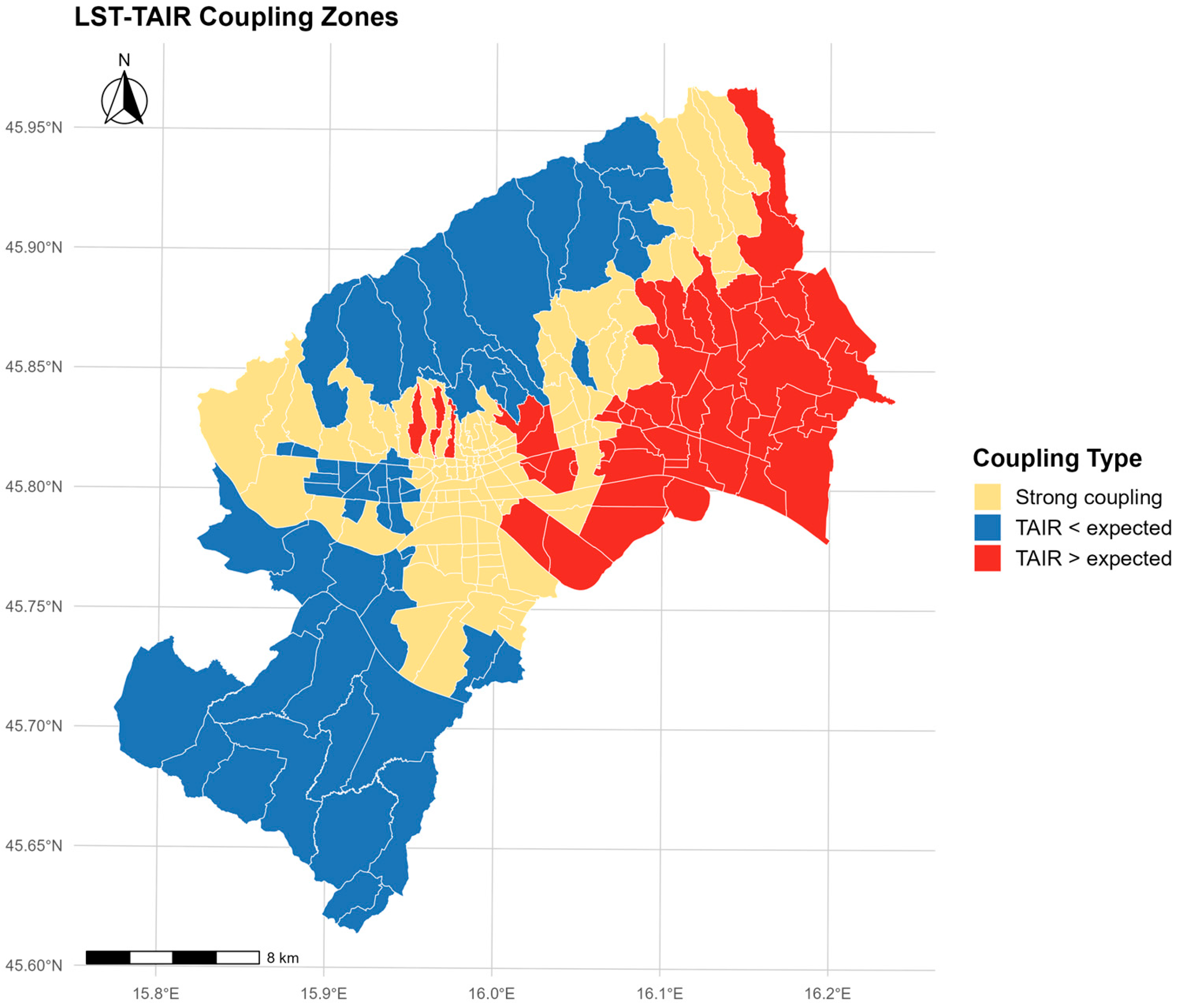
Local councils were categorized into coupling zones according to standardized residual magnitude, employing a threshold of 0.5 standard deviations. These zones were defined as follows: strong coupling (|residual| ≤ 0.5 SD, signifying that TAIR closely aligns with LST-predicted values), TAIR > expected (residual > 0.5 SD, where atmospheric heat surpasses surface-based prediction), and TAIR < expected (residual < −0.5 SD, indicating atmospheric heat is less than surface-based prediction). This 0.5 SD threshold represents a moderate criterion, balancing sensitivity to meaningful local deviations against over-classification of minor statistical noise while maintaining sufficient sample sizes in each category for spatial pattern interpretation.

3.5.3. Spatial Overlap of Hot Spots

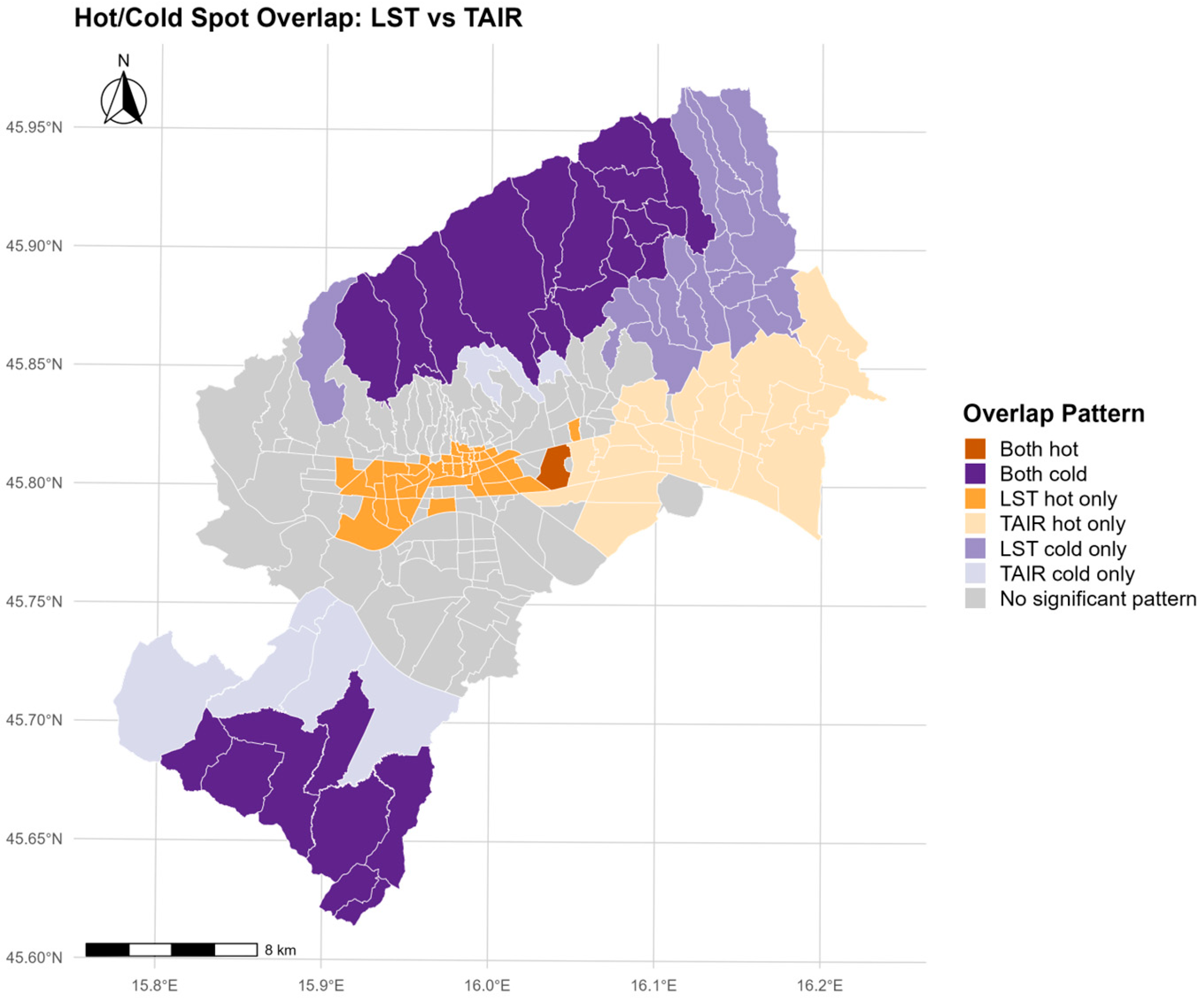
To distinguish convergent heat zones (where both surface and atmospheric heat are elevated) from divergent patterns, LST and TAIR Gi* classifications were cross-tabulated. Each local council was classified into one of seven mutually exclusive categories based on conditional logic: (1) both hot (both LST and TAIR significant hot spots, representing convergent heat), (2) both cold (both significant cold spots, representing convergent cooling), (3) LST hot only (LST hot spot but TAIR not a hot spot, surface-dominated heat), (4) TAIR hot only (TAIR hot spot but LST not a hot spot, atmosphere-dominated heat), (5) LST cold only, (6) TAIR cold only, and (7) no significant pattern (neither variable shows significant clustering). Convergent zones were defined as meteorological observations (local councils) that were classified as either “both hot” or “both cold.” This classification indicated areas where surface and atmospheric temperature extremes occurred together in space. This overlap analysis reveals the spatial extent of coupled versus decoupled thermal regimes across the city.

3.5.4. Spatial Strength Check

To assess whether OLS significance estimates were inflated by spatial autocorrelation, a spatial lag model (SLM) was estimated as: TAIR = α + β(LST) + ρW(TAIR) + ε, where ρ is the spatial autoregressive parameter and W is the row-standardized queen contiguity weight matrix, implemented using the spatialreg package (v1.3-1) in R. Model fit was compared via AIC. The presence of spatial autocorrelation in OLS residuals (Moran’s I) justified this strength check.

3.6. Land Cover Associations

3.6.1. Collinearity Assessment

Before analyzing NDVI and NDBI effects, their bivariate correlation to diagnose multicollinearity was assessed. Severe collinearity (|r| > 0.85) precludes joint inclusion in regression models, as variance inflation factors (VIFs) exceed interpretable thresholds (VIF > 10), yielding unstable coefficient estimates [33,34].

3.6.2. Separate Model Framework

Given the expected severe NDVI-NDBI collinearity in urban environments, a separate modeling strategy was adopted: Model A examines correlations of NDVI with LST and NDVI with TAIR, while Model B examines correlations of NDBI with LST and NDBI with TAIR. This method avoids the problems of multicollinearity while allowing for a formal statistical comparison of the strengths of correlations.
To test H3 (land cover is more strongly associated with LST than TAIR), correlation coefficients using Fisher’s z-transformation were compared:
z 1 = 0.5 l n 1 + r 1 1 r 1
z 2 = 0.5 l n 1 + r 2 1 r 2
Cohen’s q, a standardized measure of the difference between two Fisher-transformed correlations, was computed, where values of 0.10, 0.30, and 0.50 represent small, medium, and large effect sizes, respectively.
q = z 1 z 2
The difference between transformed correlations follows a normal distribution:
Z = z 1 z 2 1 n 3 + 1 n 3
where n = 218. One-tailed tests assessed whether |r(NDVI, LST)| > |r(NDVI, TAIR)| and |r(NDBI, LST)| > |r(NDBI, TAIR)| at α = 0.05. Convergent findings across both models provide clear conclusions for differential coupling.
It should be noted that the correlations compared via Fisher’s z-test are derived from the same 218 spatial units and share variables (LST and TAIR), meaning they are not fully independent. Results should therefore be interpreted as indicative of differential land cover associations rather than strictly independent hypothesis tests.
This section presents the findings of a sequential analysis of surface-atmospheric thermal coupling in Zagreb, organized by the research questions: spatial patterns (RQ1), the relationship between land surface temperature and air temperature (RQ2), and the differing effects of land cover (RQ3). All statistical tests used a significance level of α = 0.05.
All analyses were performed using QGIS (v3.26) and RStudio (v2023.09.1 Build 494).

4. Results

4.1. Spatial Patterns of LST and TAIR (RQ1)

4.1.1. Descriptive Statistics

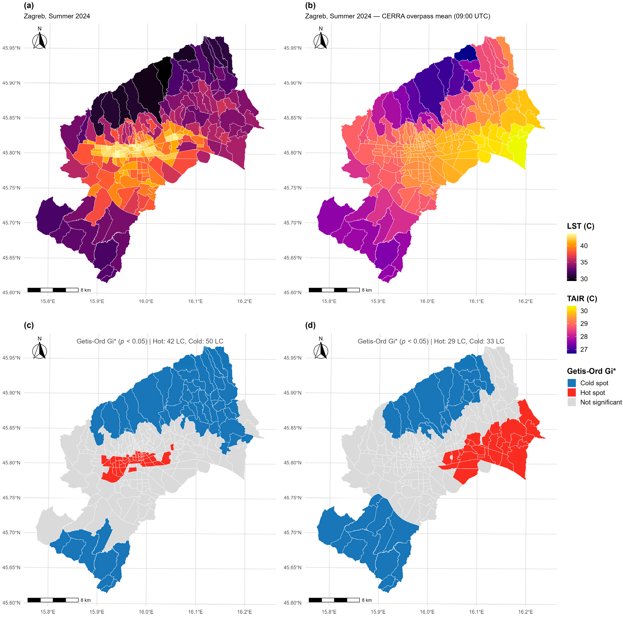
During the summer of 2024, the mean land surface temperature (LST) across Zagreb’s 218 local administrative units (local councils) exhibited a range from 29.4 °C to 43.7 °C (mean ± SD: 37.9 ± 3.7 °C, median: 38.5 °C), thereby indicating substantial spatial heterogeneity, as evidenced by a 14.3 °C difference between the coldest and hottest neighborhoods (Table 2). The distribution approximated a normal curve, albeit with a slight negative skew, which implies a tendency for higher temperature values within areas characterized by dense development. The coldest regions were primarily located in the forested peripheries, such as Maksimir and the slopes of Medvednica. The hottest areas were situated in commercial and industrial zones, which were characterized by minimal vegetation and a preponderance of impervious surfaces.
TAIR exhibited significantly reduced spatial variability, with values spanning from 26.7 °C to 30.4 °C (mean ± SD: 29.2 ± 0.7 °C, median: 29.4 °C), and a mere 3.7 °C range throughout the urban area. The distribution of TAIR was more closely concentrated around the mean, indicative of the homogenizing effects of atmospheric mixing processes that occur over areas exceeding individual neighborhoods.
This 3.9-fold disparity in range (14.3 °C versus 3.7 °C) and 5.1-fold difference in standard deviation (3.7 °C versus 0.7 °C) quantitatively substantiates LST’s heightened sensitivity to fine-scale surface heterogeneity, in contrast to TAIR’s more uniform atmospheric mixing processes. Furthermore, the coefficient of variation for land surface temperature (CV = 9.8%) exceeded that of air temperature (CV = 2.5%) by a factor of nearly four. This disparity supports the notion that atmospheric thermal characteristics exhibit greater spatial uniformity compared to surface thermal characteristics.
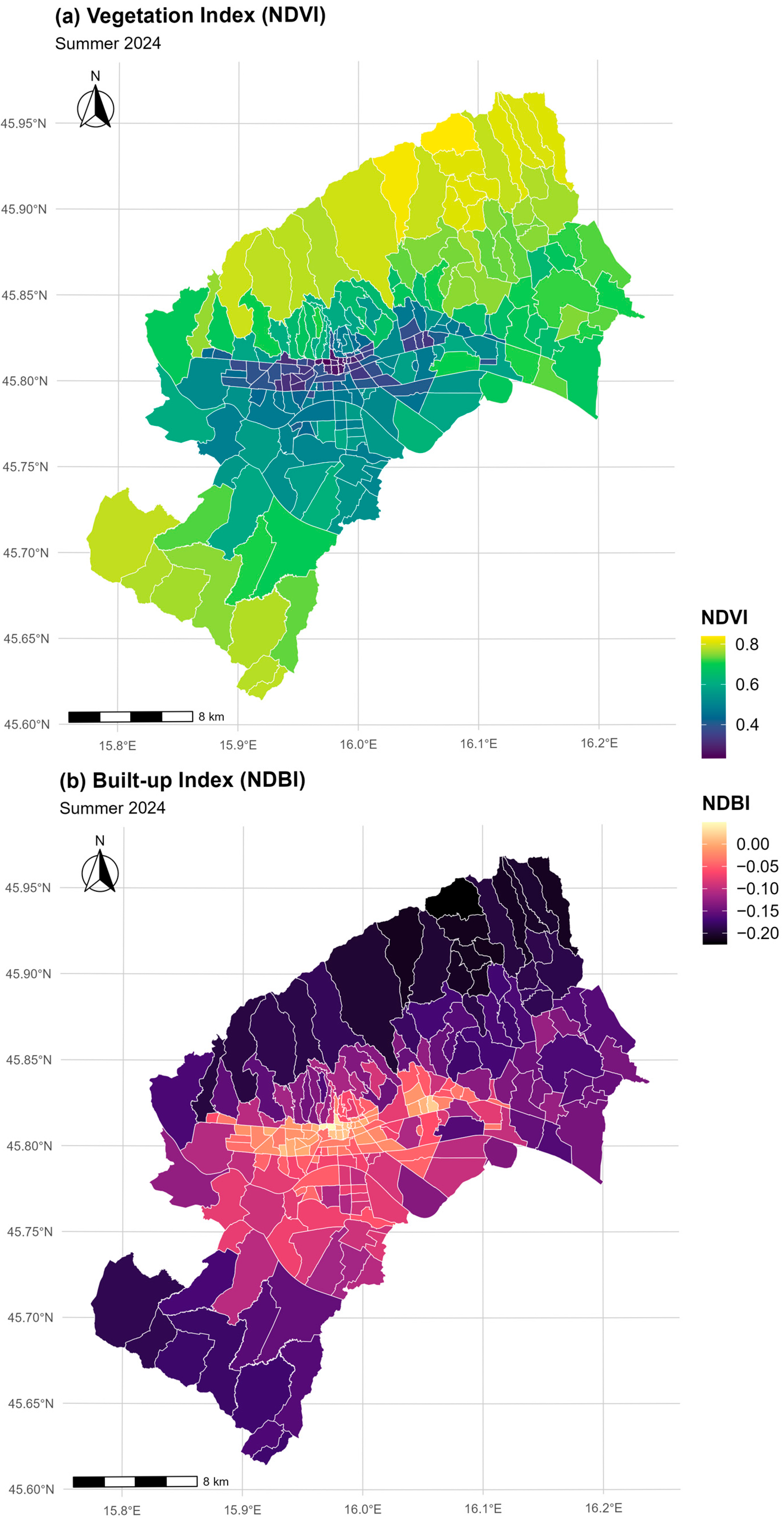
NDVI values exhibited considerable variation, spanning from 0.233 to 0.839 (mean: 0.556 ± 0.160, median: 0.547), thereby reflecting significant differences in vegetative density. These values ranged from areas with sparse vegetation in commercial zones within the urban center to regions with dense vegetation, including peripheral residential zones and urban forests situated on the slopes of Medvednica. The distribution of these values approximated symmetry, implying a relatively equal representation of both vegetated and built-up land cover types. Consequently, this extensive NDVI range effectively characterizes the heterogeneous land cover mosaic of Zagreb, encompassing areas dominated by concrete in the central business districts and regions where tree canopies are prevalent in suburban neighborhoods.
NDBI values varied from −0.225 to 0.049 (mean: −0.095 ± 0.067, median: −0.088). The preponderance of negative values suggests that Zagreb possesses a comparatively green profile when contrasted with other European capitals, as evidenced by its 23% urban forest coverage. Positive NDBI values were primarily observed in densely developed central areas, such as the Donji Grad central business district and the commercial zones of Trešnjevka, which are distinguished by continuous impervious surfaces. Conversely, negative values were indicative of vegetated suburbs and the forested periphery, where vegetation is the dominant land cover.

4.1.2. Global Spatial Autocorrelation

Both land surface temperature (LST) and air temperature (TAIR) displayed considerable positive spatial autocorrelation (Table 3), suggesting that similar temperature values were clustered within adjacent communities, as opposed to being randomly distributed across space. LST, in particular, exhibited clustering (Moran’s I = 0.767, z = 18.75, p < 0.001, variance = 0.00170), significantly surpassing the anticipated value under conditions of spatial randomness (I = −0.0046). This pronounced positive autocorrelation implies that areas with higher (or lower) LST values are likely to be situated near areas with similarly high (or low) LST values, thereby forming cohesive spatial patches that span numerous adjacent administrative units.
TAIR exhibited a more pronounced spatial clustering pattern (Moran’s I = 0.795, z = 19.52, p < 0.001), indicating a 3.6% increase in autocorrelation magnitude compared to LST. Both z-scores significantly surpassed the critical threshold for p < 0.001 (z = 3.29), thereby furnishing evidence against the null hypothesis of spatial randomness.
The observed differential autocorrelation pattern implies that atmospheric heat displays more uniform spatial gradients compared to surface heat. This is probably attributable to larger-scale atmospheric circulation, regional warming, and mesoscale advection, which occur over spatial extents (5–50 km) exceeding those of individual neighborhoods (mean area = 2.94 km2). These atmospheric phenomena generally promote the homogenization of TAIR values across extensive urban areas via horizontal mixing and vertical turbulent diffusion, thereby resulting in stronger autocorrelation.
Conversely, the slightly lower, yet still substantial, autocorrelation of LST indicates a greater degree of fine-scale heterogeneity. This is driven by local surface material characteristics (albedo values between 0.05 and 0.30, variations in thermal capacity), microscale land cover configurations (vegetation patches, building clusters), and topographic differences (elevation range from 122 to 1000 m), which generate temperature gradients at neighborhood scales (0.5–5 km).

4.1.3. Local Hot and Cold Spot Detection

Getis–Ord Gi* analysis found statistically significant clusters of very high or very low temperature values (p < 0.05, two-tailed test, |z| ≥ 1.96) across the city. These clusters had different spatial patterns for surface heat and air heat (Figure 2, Table 4). For LST, 42 local councils (19.3%) were identified as hot spots, spatial clusters of elevated surface temperatures where local values significantly surpassed the city-wide mean and were encircled by comparably elevated values. These hot spots were mostly found in commercial areas with a lot of buildings (like the Donji Grad central business district, which has 85% impervious surface coverage), industrial areas (like the eastern industrial corridor along Slavonska Avenue), places with a lot of parking lots and transportation infrastructure, and residential blocks with a lot of people and not a lot of plants. The spatial coherence of these hot spot clusters shows how heat-amplifying surface features come together at the neighborhood level. Fifty more local councils (22.9%) were found to be LST cold spots. Most of these were in vegetated suburban areas, like the Maksimir park district, which has a tree canopy that covers 70% of the area. These chilly places also included forested areas on the southern slopes of Medvednica, where dense canopy shading and evapotranspiration cause daytime surface heating to drop by 8–12 °C compared to built-up areas.
These cooler areas act as natural cooling systems, affecting surface temperatures through physical and biological processes. In contrast, the other 126 local councils (57.8%) showed no significant clustering. These areas represented transition zones, with thermal conditions similar to the average city temperature of 37.9 °C.
TAIR hot spot distributions exhibited a more restricted spatial reach and less distinct peripheral differentiation. Only 29 local councils (13.3%) were designated as hot spots, mostly located in the highly populated urban core (within a 3 km radius of the city center), and exhibiting a less extensive peripheral distribution than LST hot spots. The spatial concentration likely results from atmospheric mixing. This process reduces small temperature differences, which then hinders the formation of distinct thermal boundaries between the urban center and its surrounding areas.
The atmosphere disperses heat more effectively than the surface, which leads to smoother temperature changes instead of distinct areas of concentrated warmth. Likewise, 33 local councils (15.1%) were classified as TAIR cold spots, and 156 local councils (71.6%) demonstrated no significant clustering.
The reduced extent of significant clustering in TAIR (28.4% total) relative to LST (42.2% total) quantitatively supports the notion of a smoother spatial structure and less pronounced fine-scale temperature gradients in TAIR, aligning with the stronger global autocorrelation identified in Section 4.1.2. The spatial disparity between LST and TAIR hot spot locations offers initial evidence of a decoupling between surface and atmospheric thermal regimes. Specifically, numerous neighborhoods displayed LST hot spot status without corresponding TAIR hot spots (surface-dominated heat, N = 41 local councils), whereas other regions exhibited the opposite pattern (atmosphere-dominated heat, N = 28 local councils), thereby anticipating the divergent thermal patterns revealed through overlap analysis.
Both LST and TAIR maps use the same color palette (sequential warm color scale) to ensure visual comparability, although value ranges differ due to the inherent differences in thermal variability between surface and atmospheric temperatures (Figure 2).

4.2. LST-TAIR Spatial Coupling (RQ2)

4.2.1. Global Correlation Analysis

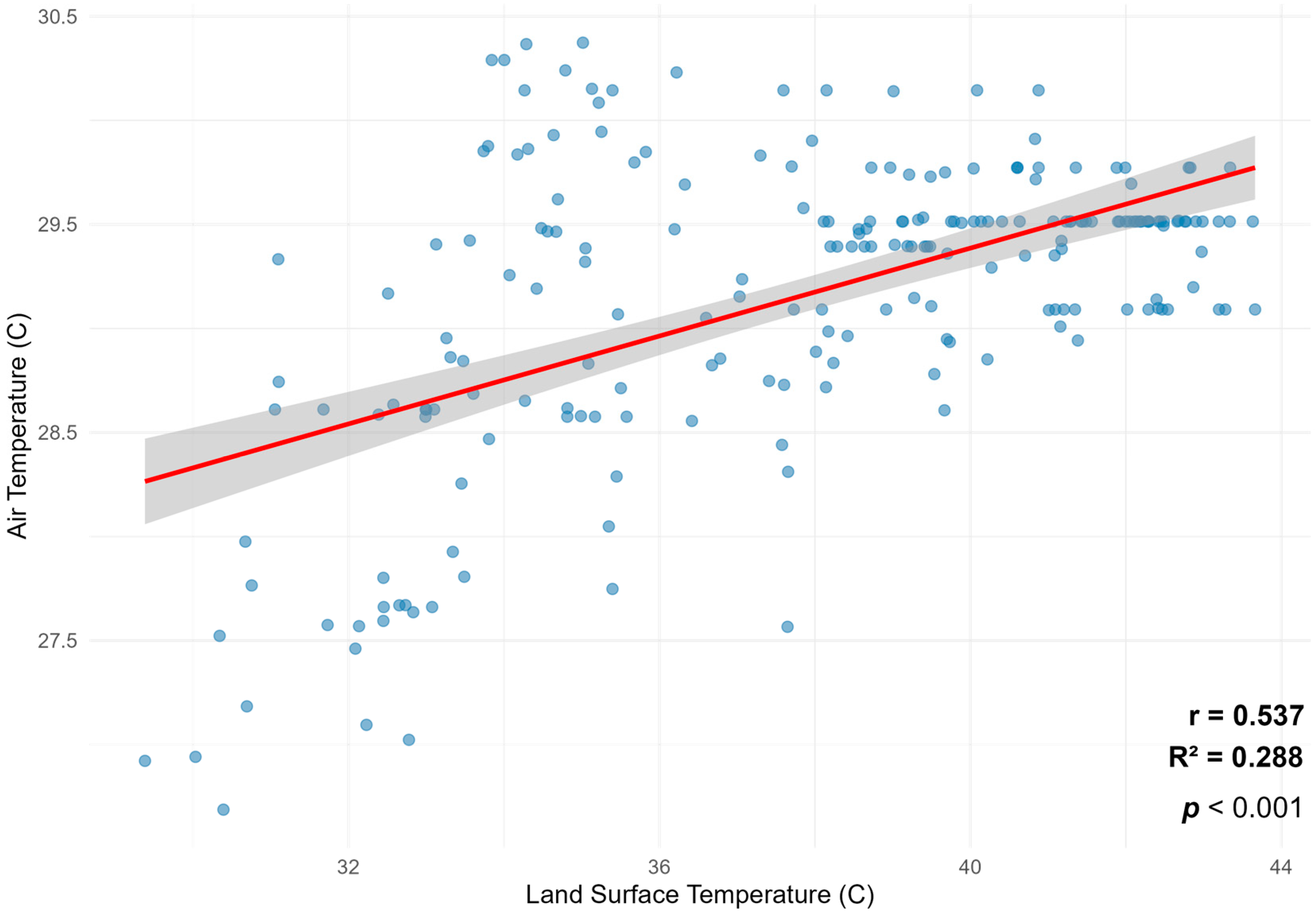
LST and TAIR showed a moderate positive correlation (r = 0.537, t = 9.35, df = 216, p < 0.001; 95% CI: [0.435, 0.625]), confirming H1’s prediction of partial coupling between surface and atmospheric thermal regimes (Figure 3). The correlation magnitude falls squarely within the partial coupling range (0.3 < r < 0.8) specified in the conceptual framework (Section 2.1), indicating that LST and TAIR share common spatial patterns but are far from identical measurements of the same underlying phenomenon. If they measured the same thermal process, correlation would approach r ≈ 1.0, if completely independent, r ≈ 0. The observed moderate coupling (r = 0.537) validates the framework’s characterization of surface and atmospheric heat as related but distinct thermal dimensions. The squared correlation coefficient (R2 = 0.288) indicates that 28.8% of spatial variance is shared between surface and atmospheric heat as a substantial proportion reflecting genuine thermal coupling through sensible heat flux from surface to atmosphere, while the remaining 71.2% reflects independent processes affecting each thermal component separately. The remaining 71.2% of the variance not accounted for reinforces the conceptual distinction between surface heat, primarily governed by solar radiation absorption, surface material properties like albedo and thermal capacity, and local land cover, and atmospheric heat, which is additionally shaped by regional circulation patterns that transport air masses across the urban environment, the advection of warm or cool air from upwind regions, and vertical mixing processes that distribute near-surface heat concentrations. Zagreb’s coupling strength, which falls within the range of strong (r > 0.7) and weak (r < 0.4) coupling, suggests a moderate relationship. While neighborhoods with elevated surface temperatures typically exhibit higher atmospheric temperatures, this is not universally applicable; certain neighborhoods deviate considerably from this trend. The positive correlation supports the notion that surface temperatures influence the atmosphere through upward heat transfer. Nevertheless, the moderate strength of this relationship implies that atmospheric processes, rather than solely land surface temperature, also contribute to the observed effects.

4.2.2. Spatial Variation in Coupling Strength

OLS regression (TAIR~LST) yielded a significant model (F(1, 216) = 68.4, p < 0.001, R2 = 0.288) with slope β = 0.106 ± 0.011 °C/°C. This indicates a 1 °C LST increase produces only a 0.11 °C TAIR increase, a ~9.4:1 attenuation reflecting weak coupling efficiency. This attenuation reflects: (1) vertical mixing diluting surface heat through the 1–2 km boundary layer; (2) horizontal advection importing air from surrounding regions; and (3) the fact that TAIR is extracted at the overpass time slot rather than a diurnal mean, meaning short-term atmospheric variability contributes to residual variance. It should also be noted that the weak OLS coupling coefficient (β = 0.106) may partly reflect the coarse spatial resolution of CERRA TAIR rather than exclusively a true physical relationship; the smoothing effect of the 5.5 km grid would tend to reduce apparent spatial variability in TAIR and thus attenuate the estimated slope. Regression residuals (range: −1.68 °C to +1.58 °C, SD = 0.62 °C) revealed substantial spatial heterogeneity, validating H2 (Figure 4). Using a 0.5 SD threshold (0.31 °C), 109 local councils (50.0%) were classified as strong coupling zones where the observed TAIR closely matched LST-predicted values. An additional 53 local councils (24.3%) showed TAIR > expected (atmospheric dominance), suggesting regional warming, warm air advection, or atmospheric stagnation. The remaining 56 local councils (25.7%) showed TAIR < expected (surface dominance/ventilation), reflecting topographic channeling, cool air drainage from Medvednica, or enhanced mixing (Table 5).
Spatial autocorrelation in OLS residuals (Moran’s I = 0.769, p < 0.001) confirmed that standard errors may be underestimated under OLS. A spatial lag model yielded ρ = 0.931 and a substantially improved fit (AIC: OLS = 412.0 vs. SLM = 93.7), while the LST coefficient declined from β = 0.106 to β = 0.025 after accounting for spatial dependence. This confirms that the OLS coupling estimate reflects genuine surface-to-atmosphere association, but its magnitude should be interpreted cautiously given strong spatial autocorrelation in both variables.

4.2.3. Hot Spot Overlap Analysis

Cross-tabulation of LST and TAIR Gi* classifications revealed limited spatial overlap between surface and atmospheric thermal extremes, providing strong support for H2’s prediction of distinct thermal dimensions (Table 6, Figure 5). Only one local council (0.5%) was classified as a hot convergent heat zone where both LST and TAIR exhibited significant hot spot clustering (p < 0.05 for both Gi* statistics). These zones represent the most thermally stressed neighborhoods where surface and atmospheric heat extremes spatially coincide, creating compounded thermal burden. These areas likely require priority intervention for heat mitigation given the convergence of both thermal stress dimensions. Similarly, only 25 local councils (11.5%) showed both cold patterns, representing convergent cooling zones where both surface and atmospheric cold spots overlap. These neighborhoods benefit from dual cooling mechanisms operating at both thermal levels. Combining these categories, convergent zones comprised merely 26 local councils (11.9%) of the city, approximately one-ninth of all neighborhoods. This limited convergence is substantially below what would be expected if LST and TAIR operated in perfect spatial lockstep (which would yield ~100% convergence) but above the statistical expectation under complete independence (19.3% × 13.3% = 2.6% for hot spots, 22.9% × 15.1% = 3.5% for cold spots, totaling ~6% convergence). In contrast, divergent patterns where only one thermal component showed significant clustering were substantially more common. Forty-one local council (18.8%) showed LST hot only patterns, indicating surface-dominated heat where elevated surface temperatures do not translate into atmospheric thermal burden. These areas might indicate effective vertical mixing, which prevents atmospheric heat from building up despite the presence of hot surfaces, or a time lag where daytime surface heating dissipates before significantly affecting near-surface-atmospheric temperature at the overpass time. Conversely, 28 local councils (12.8%) showed only hot TAIR patterns, indicating heat primarily from the atmosphere, separate from local surface conditions. These areas might be influenced by the movement of warm air from upwind heat sources, or by regional atmospheric warming that outweighs local surface cooling. Cold spot divergence was also observed: 20 local councils (9.2%) for LST cold only and eight local councils (3.7%) for TAIR cold only. The remaining 95 local councils (43.6%) showed no significant clustering in either variable. Quantitatively, this limited convergence (11.9%) versus substantial divergence (44.5% showing single-component extremes) confirms that LST and TAIR represent distinct thermal dimensions of the urban environment, strongly supporting H2. If surface and atmospheric heat operated in perfect spatial lockstep, convergence would approach 100% and divergence would approach 0%; if they were completely independent, convergence would match the product of marginal probabilities (~6%) and divergence would reflect independent occurrences. The observed pattern falls between these extremes but considerably closer to independence than to perfect coupling. This divergence pattern has critical implications for heat mitigation strategies: interventions targeting surface cooling (e.g., increasing surface albedo through cool pavements, expanding tree canopy to provide shading) may not proportionally reduce atmospheric thermal exposure for urban residents, and conversely, atmospheric interventions (e.g., promoting air circulation through urban design) may not address surface thermal stress. Therefore, a variety of multi-level approaches are needed to address both surface and atmospheric heat, using combined, not just single, strategies.
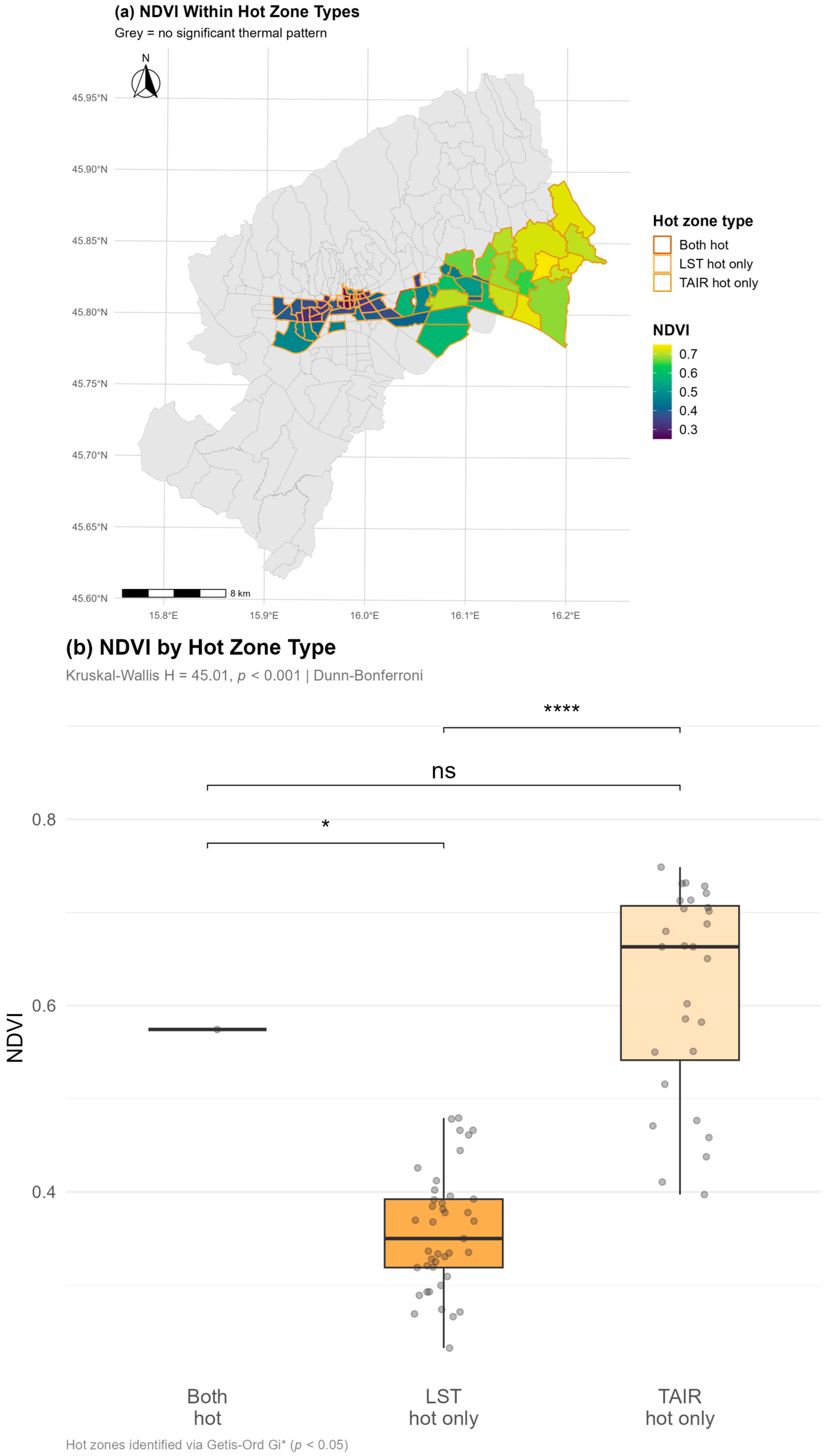
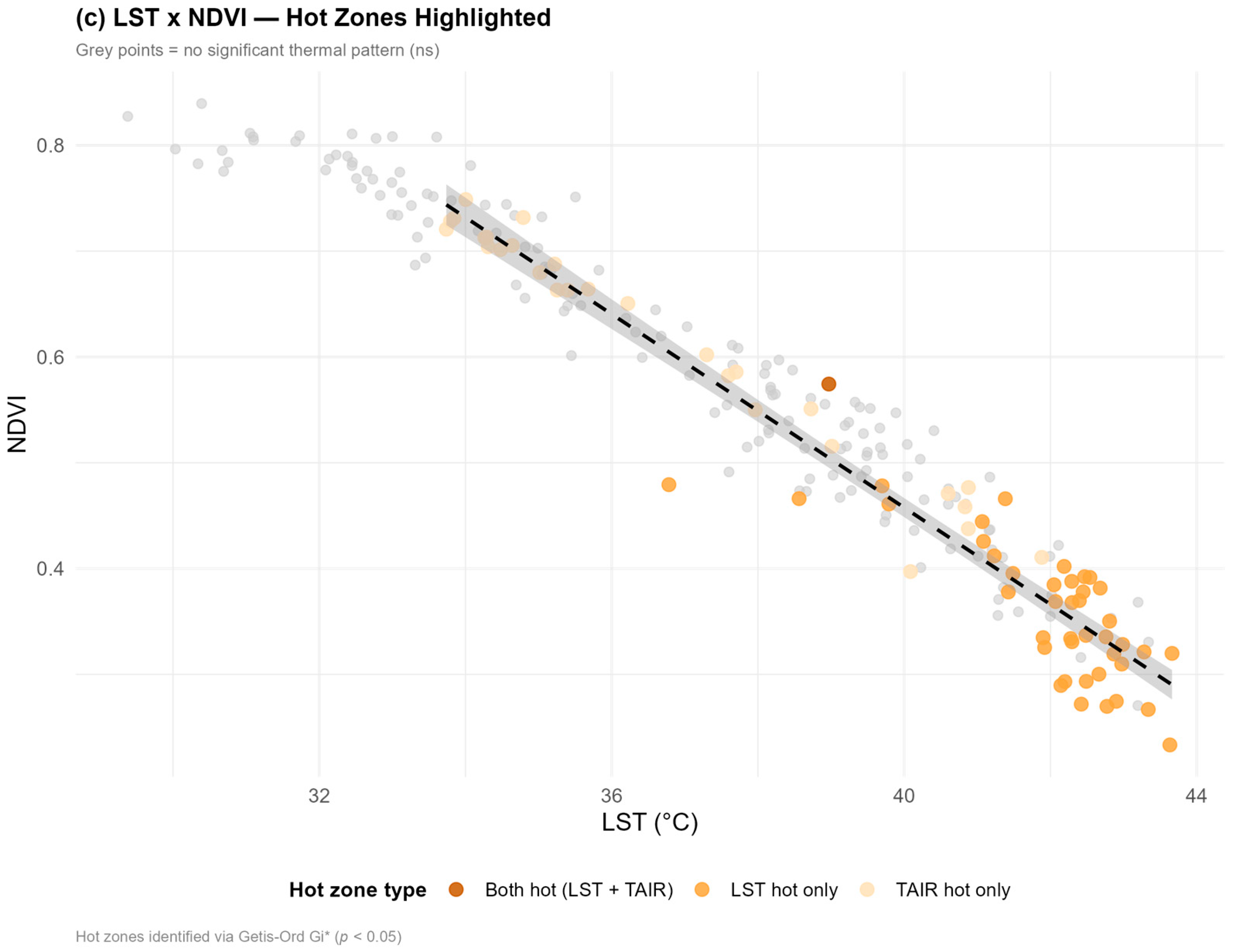
To further contextualize the spatial divergence between LST and TAIR hot spots identified above, NDVI was compared across hot spot overlap categories (Figure 6). Results revealed statistically significant differences in vegetation cover between zone types (Kruskal–Wallis H = 45.02, df = 2, p < 0.001). Given that only one local council was classified as both hot, this category was retained as a descriptive reference point only; formal comparisons were conducted between LST hot only and TAIR hot only zones. LST-dominant hot spots exhibited a markedly low vegetation cover (median NDVI = 0.350), substantially below TAIR-exclusive hot spots (median NDVI = 0.663), with this difference statistically significant (Dunn test, p < 0.001). Spatially, LST hot only zones cluster in the densely built western urban core: predominantly the Trešnjevka area, characterized by high impervious surface cover, low canopy density, and minimal green space. In contrast, TAIR-exclusive hot spots extend eastward into neighborhoods that retain moderate to high vegetation cover but are exposed to atmospheric heat accumulation through mechanisms unrelated to local surface conditions, such as reduced ventilation, higher building density, or advection from upwind heat sources. This east–west thermal contrast reflects Zagreb’s broader urban morphological gradient: the western districts, developed largely during socialist-era mass housing construction, are characterized by high building coverage ratios and fragmented green space, producing strong LST signals. Eastern neighborhoods, though more recently developed and partially vegetated, remain thermally exposed at the atmospheric level as a distinction invisible to surface-only thermal analyses and relevant for targeted urban climate adaptation (Figure 6).

4.3. Differential Land Cover Effects (RQ3)

4.3.1. NDVI-NDBI Collinearity

NDVI and NDBI exhibited severe negative collinearity (r = −0.991, p < 0.001), confirming they capture a single vegetated-to-built-up gradient rather than independent characteristics. This near-perfect correlation (r2 = 0.982) would yield VIF = 55.6 if jointly modeled, far exceeding multicollinearity thresholds (VIF > 10). Consequently, they were analyzed in separate models (Model A: NDVI; Model B: NDBI) to enable valid inference while preserving ability to test differential coupling through Fisher’s z-tests. This avoids collinearity pathologies while allowing formal hypothesis testing.

4.3.2. Model A: NDVI Differential Associations

NDVI (Figure 7a; Table 7) showed a very strong negative correlation with LST (r = −0.970, p < 0.001, R2 = 0.941), demonstrating vegetation as the dominant surface temperature predictor, explaining 94.1% of LST variance. High-canopy neighborhoods (NDVI > 0.7) were 10–12 °C cooler than sparse-vegetation districts (NDVI < 0.3), reflecting combined effects of canopy shading, evapotranspiration, and higher albedo. NDVI–TAIR correlation was considerably weaker (r = −0.478, p < 0.001, R2 = 0.228), representing a 51% reduction in correlation magnitude and a 76% reduction in explained variance. While statistically significant, vegetation’s atmospheric effect is substantially attenuated by mixing and broader-scale atmospheric processes. Fisher’s z-test (z = 16.341, p < 0.001, Cohen’s q = 1.576; Table 7) confirmed a significantly stronger association with LST, supporting the interpretation that vegetation primarily modulates surface thermal properties through direct biophysical mechanisms, while its atmospheric influence is moderated by larger-scale processes.

4.3.3. Model B: NDBI Differential Associations

NDBI (Figure 7b; Table 7) demonstrated a very strong positive correlation with LST (r = +0.973, p < 0.001, R2 = 0.947), indicating impervious surfaces as the dominant surface warming driver, explaining 94.7% of LST variance. High built-up intensity (NDBI > 0) yielded LST values 10–14 °C warmer than vegetated areas (NDBI < −0.15), reflecting low albedo, high thermal capacity, anthropogenic heat emissions, and reduced evapotranspiration. The correlation between NDBI and TAIR was considerably weaker (r = +0.496, p < 0.001, R2 = 0.246), representing a 49% decrease in correlation strength and a 74% reduction in explained variance, consistent with the NDVI results. Furthermore, Fisher’s z-test (z = 16.583, p < 0.001, Cohen’s q = 1.599; Table 7) confirmed a significantly stronger association with LST, supporting the interpretation that impervious surfaces primarily influence surface thermal properties, while atmospheric effects are moderated by larger-scale processes.

4.3.4. Hypothesis Testing Summary

Convergent evidence supports H3: land cover is more strongly associated with LST than TAIR (Table 7). Both indices show 64–67% reductions in explained variance for atmospheric versus surface associations (p < 0.001). Near-identical attenuation despite opposite correlation directions provides particularly strong validation. This confirms land cover characteristics primarily modulate surface thermal properties through direct physical mechanisms at the land–atmosphere interface, while atmospheric heat is additionally influenced by broader-scale processes (regional circulation, horizontal advection, vertical mixing through 1–2 km boundary layer) that attenuate local land cover signals by approximately two-thirds. The separate model framework enabled valid inference despite collinearity, providing convergent evidence that land cover effects operate primarily at the surface level (~95% variance explained) rather than the atmospheric level (~35%). Implications: Increasing vegetation or reducing impervious surfaces produces large surface reductions (~10–12 °C possible) but modest atmospheric reductions (~2–3 °C), suggesting land cover interventions should complement atmospheric-scale strategies (promoting air circulation, regional greening) to achieve comprehensive thermal stress reduction.

5. Discussion

The findings of this research indicate that surface and atmospheric urban heat constitute interconnected, though separate, thermal characteristics. The observed partial correlation (r = 0.537, R2 = 0.288) situates Zagreb within a spectrum ranging from complete thermal integration (r ≈ 1.0) to full decoupling (r ≈ 0). This observation supports the characterization of urban heat as a multi-dimensional phenomenon, thereby necessitating varied analytical and intervention strategies.

5.1. Surface-Atmospheric Thermal Decoupling

The 71.2% unexplained variance between LST and TAIR demonstrates that surface thermal conditions do not directly translate into atmospheric exposure. This aligns with previous studies documenting weak-to-moderate LST-TAIR correlations in urban environments [1,4,6], with coupling strength varying by season, time of day, and land cover characteristics [2,3]. Our hot spot overlap analysis provides spatial specificity: only 11.9% of neighborhoods exhibited convergent thermal extremes, while 44.5% showed divergent patterns. This reveals that surface heat islands do not necessarily coincide with atmospheric heat islands, with critical implications for heat vulnerability assessment.
Three physical processes contribute to this decoupling. Initially, vertical mixing, which occurs within the 1–2 km boundary layer, disperses surface heat, thereby distributing energy over a more extensive air volume [51,52]. Secondly, horizontal advection, which brings in air masses from adjacent areas, is significant in Zagreb, considering its location in the Sava valley and its proximity to Medvednica mountain. Finally, residual temporal asynchrony between the instantaneous daytime LST measurement at the satellite overpass (~09:45 UTC) and the CERRA T2m slot at 09:00 UTC introduces a small but non-negligible offset; while this mismatch is substantially reduced compared to daily mean approaches, the ~45 min difference may contribute to residual decoupling during periods of rapid morning surface heating [2,3]. Table 8 summarizes the principal physical mechanisms contributing to LST–TAIR spatial decoupling, organized by spatial scale and relative contribution to the observed divergence patterns [2,3,51,52].
The magnitude of LST–TAIR decoupling is further modulated by urban form and seasonality; recent work has demonstrated that the relationship between surface and air temperature varies substantially across local climate zones and seasons, with the strongest divergence occurring in densely built environments during summer.

5.2. Differential Land Cover Effects

Land cover shows dramatically stronger association with surface heat (NDVI-LST: r = −0.970, R2 = 0.941; NDBI-LST: r = +0.973, R2 = 0.947) than atmospheric heat (NDVI-TAIR: r = −0.478, R2 = 0.228; NDBI-TAIR: r = +0.496, R2 = 0.246). Vegetation and built-up intensity explain ~95% of surface variance but only ~24% of atmospheric variance: a 74–76% reduction. This confirms land cover primarily modulates surface thermal properties through direct biophysical mechanisms including evapotranspiration, shading, and albedo modification [14,15,17], while atmospheric heat is additionally influenced by broader-scale processes.
The nearly perfect inverse relationship between NDVI and NDBI (r = −0.991) indicates that urban areas exist along a continuous spectrum from vegetation to built environments, rather than as separate land cover types [19,20]. The consistency of results across both models is characterized by similar reductions in variance despite opposing correlation directions and supports the notion that this differential coupling is indicative of actual physical processes, rather than methodological biases. Furthermore, Fisher’s z-tests revealed significantly stronger surface associations for both indices (p < 0.001), with substantial effect sizes (Cohen’s q ≈ 1.6).
Practically, higher vegetation cover is associated with substantially lower surface temperatures (~10–12 °C across the observed NDVI/NDBI range) but with considerably smaller atmospheric temperature differences (~1–2 °C). This disparity suggests that the strong land cover–surface temperature associations observed here may not translate proportionally into atmospheric heat reduction, underscoring the potential need for supplementary approaches targeting regional circulation [17,18]. The weak surface-to-air coupling efficiency (β = 0.106, indicating that a 1 °C difference in LST corresponds to only a 0.11 °C difference in TAIR) quantifies this attenuated relationship between surface and atmospheric thermal conditions. Recent mesoscale modeling corroborates that vegetation cooling demonstrates specific diurnal patterns, with evapotranspiration effects most pronounced during daylight hours but lessening at night [17], thereby elucidating the surface-atmosphere cooling asymmetry.
The spatial distribution of NDVI within the defined thermal overlap categories offers further mechanistic understanding of this decoupling phenomenon. LST hot only zones recorded a median NDVI of 0.350, corroborating the strong association between surface heat extremes and vegetation deficits. This finding aligns with the established influence of impervious surfaces on urban LST, which is mediated by reduced latent heat flux, increased sensible heat storage, and lower albedo [25,28,30]. The western urban core, including Trešnjevka, exemplifies this pattern: high-density residential development with limited tree canopy creates a persistent surface heat signature that is clearly legible in both LST values and NDVI deficits. More theoretically significant is the TAIR hot only finding. These zones, with a median NDVI of 0.663 substantially exceeding thermally neutral areas (0.514), demonstrate that atmospheric heat accumulation can occur independently of local vegetation deficit. This decoupling suggests that TAIR hot spots are governed by mesoscale or morphological processes: restricted airflow through canyon geometries, thermal inertia of building mass, or advection of warm air masses from the densely built core toward the urban periphery [51,52]. The eastward extension of TAIR-exclusive hot spots into more vegetated neighborhoods is particularly notable, as it implies that greening strategies alone would be insufficient to address atmospheric heat exposure in these areas. Residents in TAIR hot zones face an elevated thermal burden despite the presence of vegetation; a finding with direct relevance for heat health risk assessment and the spatial targeting of cooling interventions [53].

5.3. Spatial Heterogeneity

The identified coupling/decoupling zones demonstrate spatial heterogeneity that is obscured by aggregate metrics. Neighborhoods exhibiting TAIR values exceeding expectations (24.3%) might necessitate atmospheric-scale interventions designed to enhance air circulation. Conversely, zones with TAIR values below expectations (25.7%) could already be experiencing the advantages of beneficial mixing, notwithstanding elevated surface temperatures. Consequently, this allows for the implementation of targeted strategies tailored to local thermal regimes, as opposed to the application of uniform, city-wide policies.
Divergent thermal patterns are crucial for evaluating vulnerability. Current methods often rely solely on land surface temperature (LST) because of its wide coverage [54]. Our findings show that using surface heat alone provides an incomplete picture: 12.8% of neighborhoods had atmospheric hot spots without surface hot spots, indicating a risk that LST-only assessments miss. Conversely, 18.8% of the areas had surface-only hot spots, where thermal stress might not lead to atmospheric problems. This difference, 44.5% of the city showing extreme conditions in one dimension compared to only 11.9% in areas with both, demonstrates that relying solely on satellite-derived LST systematically misrepresents thermal exposure in nearly half of the neighborhoods.
Comprehensive mapping should integrate both LST and spatially interpolated TAIR data [7,8] to avoid systematic risk under/overestimation in atmosphere-dominated or surface-dominated zones.
Methodologically, our approach, which uses separate models and Fisher’s z-tests, offers a way to analyze land cover indices that are highly correlated, while still being statistically sound. The strong collinearity between NDVI and NDBI (r = −0.991, VIF = 55.6) would make it difficult to get reliable results from a combined regression. However, using separate models allowed us to make valid inferences by comparing correlations independently. This method can be used in other urban environments where predictor collinearity makes multivariate analysis more complex.

5.4. Limitations

Several limitations should be acknowledged. Although TAIR was extracted at the overpass time slot to minimize temporal mismatch, the CERRA product at 5.5 km native resolution cannot resolve fine-scale intra-neighborhood atmospheric variability, and the validation was constrained to the two official main meteorological stations operating within the City of Zagreb as the only available in situ network for the study area. Future research utilizing dense sensor networks [4] or high-resolution downscaling methodologies [8,9,10] might yield a more detailed atmospheric characterization. The summer 2024 snapshot restricts the generalizability of the findings across diverse climatic conditions, given that LST-TAIR relationships demonstrate seasonal variability [3,5]; it is expected that coupling strength and spatial patterns would differ substantially in winter, when reduced solar radiation attenuates surface heating and atmospheric processes dominate. Furthermore, the cross-sectional design precludes causal inference; however, convergent evidence from multiple approaches offers strong support for the proposed relationships. Future research endeavors should investigate the temporal coupling dynamics present within both diurnal and seasonal cycles [5,6], examine the variability of coupling in relation to synoptic weather patterns, and assess the impacts of land cover interventions employing longitudinal methodologies. Extending this framework to include multiple urban areas across varied climate zones would clarify whether partial coupling represents a universal phenomenon or one that is dependent on particular contextual factors. Furthermore, the incorporation of three-dimensional urban morphology data [55,56] could enhance the comprehension of how the built environment influences surface-atmosphere heat transfer.
Reanalysis products are recognized as carrying systematic biases in urban environments, primarily because their underlying land surface models lack sophisticated urban parameterizations that capture the modified energy balance of built-up areas [57,58]. Assessments of ERA5 over Paris have demonstrated that the reanalysis fails to reproduce the surface urban heat island without dedicated urban canopy schemes, with daytime LST biases exceeding 8 °C degrees over urban grid cells [57]. The higher-resolution CERRA product (5.5 km) has been shown to outperform ERA5 for 2 m air temperature across Europe, achieving an RMSE of 0.95 K against 1064 stations [59], with particularly strong performance during the warm season and in regions of complex topography [60,61]. Bias correction of reanalysis T2m has been shown to be especially important for urban locations, where the ERA5 bias is more pronounced than at rural sites [58]. In the present study, the station-based validation (Table 1) yielded biases ranging from +0.06 °C to −0.35 °C across three validation schemes—magnitudes that fall well below the uncertainty range of the Landsat-derived LST (±1–2 °C). Because the core analyses rely on relative spatial patterns and correlation structures rather than on absolute temperature values, systematic bias correction was not applied; at the observed bias magnitudes, correction would not alter the direction or magnitude of the reported spatial associations.

5.5. Concluding Discussion Remarks

Surface and atmospheric urban heat, despite their positive correlation, constitute separate thermal dimensions that necessitate distinct frameworks and interventions. This conceptual distinction is supported by the moderate coupling (r = 0.537), the limited spatial overlap (11.9% convergence), and the differing effects of land cover, with 95% versus 24% of the variance explained. Therefore, strategies to reduce heat must address both aspects at the same time, using complementary methods. These include changing land cover to cool surfaces [14,15,17,18], along with urban design that encourages air movement. In contrast, approaches that focus on only one aspect risk incomplete cooling and potential bias in vulnerability assessments. This highlights the need for combined surface-atmosphere frameworks in climate adaptation planning.

6. Conclusions

This research underscores the fundamentally different thermal characteristics of surface and atmospheric urban heat, thereby necessitating distinct analytical and intervention approaches. A thorough spatial analysis of 218 local councils in Zagreb during the summer of 2024 revealed a partial coupling between land surface temperature (LST) and air temperature (TAIR) (r = 0.537, R2 = 0.288), with 71.2% of the spatial variance not accounted for by their linear relationship—a proportion that reflects both genuine physical decoupling and residual measurement uncertainty inherent in comparing satellite-derived LST with reanalysis-based TAIR. This moderate coupling, situated between complete thermal integration (r ≈ 1.0, where surface and atmospheric heat would be interchangeable measurements) and full decoupling (r ≈ 0, where they would be independent phenomena), supports the conceptual framework that differentiates surface heat primarily influenced by radiation absorption, surface material properties, and local land cover composition from atmospheric heat, which is also affected by regional circulation patterns, horizontal advection, and boundary layer mixing processes operating at spatial scales of 5–50 km. The observed coupling strength, which falls within the partial coupling range (0.3 < r < 0.8) defined in our conceptual framework, confirms that surface and atmospheric thermal conditions share spatial patterns, even though they are distinct indicators of urban thermal stress.
Three research hypotheses were rigorously evaluated and substantiated through the application of several complementary analytical methodologies. Initially, hot spot overlap analysis, employing Getis–Ord Gi* statistics, indicated a limited degree of spatial convergence; specifically, only 11.9% of neighborhoods displayed concurrent LST and TAIR hot/cold spots. Conversely, a considerable divergence was observed, with 44.5% of the areas exhibiting single-dimension thermal extremes, where significant clustering was confined to either surface or atmospheric heat. This observed pattern corroborates the notion that surface heat islands do not invariably coincide with atmospheric heat islands in the majority of urban settings, thereby validating H2’s assertion regarding the distinctiveness of thermal dimensions. Furthermore, the effects of land cover demonstrated a strikingly differential association: vegetation (NDVI) and built-up intensity (NDBI) accounted for approximately 95% of surface temperature variance (R2 = 0.941 and 0.947, respectively), yet only ~24% of atmospheric variance (R2 = 0.228 and 0.246), representing a 74–76% reduction in explanatory power when transitioning from surface to atmospheric thermal metrics.
Fisher’s z-tests confirmed these differences were statistically significant (p < 0.001) with large effect sizes (Cohen’s q ≈ 1.6), strongly supporting H3. Third, the observed partial coupling combined with spatially heterogeneous coupling/decoupling zones (50% strong coupling, 24.3% atmospheric dominance, 25.7% surface dominance) validated that surface and atmospheric thermal regimes operate as related but distinct phenomena requiring differentiated analytical frameworks, confirming H1.
These results have significant implications for policies aimed at mitigating urban heat. The observed associations suggest that land cover modifications, such as vegetation expansion and impervious surface reduction are strongly linked to surface thermal conditions, but their relationship with atmospheric heat is substantially weaker, with the surface-to-air coupling efficiency quantified at β = 0.106, indicating that a 1 °C change in LST is associated with only a 0.11 °C change in TAIR. This attenuated relationship implies that land cover interventions, while beneficial for surface cooling, may offer more limited atmospheric heat mitigation absent supplementary strategies targeting regional air circulation. These findings should be interpreted as evidence of strong spatial associations rather than direct causal estimates of intervention outcomes.
These findings fundamentally challenge the common practice of using satellite-derived land surface temperature (LST) as the only measure of how people experience heat. The spatial disaggregation of thermal extremes reveals systematic characterization errors. Analysis identified 12.8% of neighborhoods (28 local councils) showing atmospheric hot spots without corresponding surface hot spots, representing thermal risk that would be completely invisible in LST-only assessments and leading to systematic underestimation of vulnerability in these atmosphere-dominated zones. Conversely, 18.8% of neighborhoods (41 local councils) exhibited surface-only hot spots where elevated LST does not translate into atmospheric thermal burden, potentially leading to overestimation of actual human heat exposure in these surface-dominated zones with efficient atmospheric mixing or ventilation. This divergence pattern, affecting 44.5% of the city where single-dimension extremes occur versus only 11.9% showing convergent patterns, demonstrates that reliance on satellite-derived LST alone systematically mischaracterizes thermal exposure conditions in nearly half of urban neighborhoods. Comprehensive vulnerability mapping must integrate both surface temperature data (from satellite remote sensing providing high spatial resolution) and atmospheric temperature data (from spatial interpolation of meteorological measurements or high-resolution modeling) to avoid systematic risk under/overestimation in atmosphere-dominated or surface-dominated zones. This integration is particularly critical for identifying priority intervention areas and targeting heat-vulnerable populations.
To address the severe collinearity between NDVI and NDBI (r = −0.991), separate-model frameworks with Fisher’s z-tests were used. This approach allowed for reliable conclusions while avoiding the instability that can occur in joint regression. This method can be applied to other situations where predictor collinearity complicates multivariate analysis.
To enhance the generalizability of these findings, future research endeavors should expand the framework’s applicability to include a wider range of urban settings and climatic zones. A more thorough understanding of heat transfer mechanisms could be attained by investigating coupling dynamics during heatwaves, integrating three-dimensional urban morphology, and conducting long-term evaluations of implemented strategies. Furthermore, the constraints associated with reanalysis-based air temperature data could be mitigated through the deployment of dense sensor networks or the utilization of high-resolution modeling methodologies.
In summation, a successful approach to mitigating urban heat necessitates an understanding that surface and atmospheric heat represent separate intervention targets. Modifications to land cover, such as vegetation expansion, albedo enhancement, and impervious surface reduction, are strongly associated with surface thermal conditions. Conversely, urban design strategies, including air circulation corridors, enhanced ventilation, and regional greening, address atmospheric heat exposure. Approaches that focus solely on one dimension, whether surface greening or atmospheric circulation, are likely to result in incomplete thermal stress reduction and a biased assessment of vulnerability. The need for integrated surface-atmospheric frameworks in climate adaptation planning is evident; comprehensive thermal stress reduction requires multi-level interventions that operate at both the land–atmosphere interface and broader atmospheric scales. The observed attenuation ratio (β = 0.106) suggests that local interventions, while effective in reducing surface temperatures, provide only limited atmospheric benefits without the implementation of complementary regional strategies.
Urban climate adaptation requires integrated frameworks that specifically address both thermal dimensions. These frameworks should involve coordinated, multi-scale strategies that combine local land cover changes with regional atmospheric approaches. This is not just a matter of optimization; it is crucial for significantly reducing surface and atmospheric thermal stress. Such an approach is essential for safeguarding vulnerable populations and constructing climate-resilient cities in the face of escalating urban heat.

Author Contributions

Conceptualization, D.B. and M.G.; methodology, D.B. and M.G.; software, D.B.; validation, D.B. and M.G.; formal analysis, D.B.; investigation, D.B.; resources, D.B.; data curation, D.B. and M.G.; writing—original draft preparation, D.B.; writing—review and editing, M.G.; visualization, D.B.; supervision, M.G.; project administration, D.B. and M.G.; funding acquisition, M.G. All authors have read and agreed to the published version of the manuscript.

Funding

This study was supported by the Croatian Science Foundation ALCAR project “Assessment of the Long-term Climatic and Anthropogenic Effects on the Spatio-temporal Vegetated Land Surface Dynamics in Croatia using Earth Observation Data” (Grant No. HRZZ IP-2022-10-5711), and supported and funded by the project “Advanced Methods of Photogrammetry and Remote Sensing for Monitoring Changes in the Environment (RS4ENVIRO)”, funded through the National Recovery and Resilience Plan (NRRP/NPOO) and financed by the European Union—NextGenerationEU.

Data Availability Statement

The Landsat surface temperature data used in this study are publicly available from the United States Geological Survey (USGS) EarthExplorer platform. Atmospheric temperature data from the Copernicus Regional Reanalysis for Europe (CERRA) are openly accessible through the Copernicus Climate Data Store. Neighborhood-level demographic data for Zagreb (2001, 2021) were obtained from the City of Zagreb.

Conflicts of Interest

The authors declare no conflicts of interest.

References

  1. Jaber, S.M.; Sengupta, R. Spatial and temporal variabilities in land surface temperatures and near-surface air temperatures in an arid to semiarid urban region: Implications for urban heat island research. Geo-Spat. Inf. Sci. 2024, 27, 2137–2161. [Google Scholar] [CrossRef] [Scilit]
  2. Schwarz, N.; Lautenbach, S.; Seppelt, R. Exploring indicators for quantifying surface urban heat islands of European cities with MODIS land surface temperatures. Remote Sens. Environ. 2011, 115, 3175–3186. [Google Scholar] [CrossRef] [Scilit]
  3. Li, X.; Zhou, Y.; Asrar, G.R.; Zhu, Z. The Impact of Seasonality and Land Cover on the Consistency of Relationship between Air Temperature and LST Derived from Landsat 7 and MODIS at a Local Scale: A Case Study in Southern Ontario. Land 2021, 10, 672. [Google Scholar] [CrossRef] [Scilit]
  4. Chakraborty, T.; Venter, Z.S.; Qian, Y.; Lee, X. Crowdsourced air temperatures contrast satellite measures of the urban heat island and its mechanisms. Sci. Adv. 2021, 7, eabb9569. [Google Scholar] [CrossRef] [Scilit]
  5. Scott, A.A.; Waugh, D.W.; Zaitchik, B.F. The Dynamic Relationship between Air and Land Surface Temperature within the Madison, Wisconsin Urban Heat Island. Remote Sens. 2022, 14, 165. [Google Scholar] [CrossRef] [Scilit]
  6. Naserikia, M.; Hart, M.A.; Nazarian, N.; Bechtel, B.; Lipson, M.; Nice, K.A. Land surface and air temperature dynamics: The role of urban form and seasonality. Sci. Total Environ. 2023, 905, 167306. [Google Scholar] [CrossRef] [Scilit] [PubMed]
  7. Guo, Y.; Unger, J.; Khabibolla, A.; Tian, G.; He, R.; Li, H.; Gál, T. Modeling urban air temperature using satellite-derived surface temperature, meteorological data, and local climate zone pattern—A case study in Szeged, Hungary. Theor. Appl. Climatol. 2024, 155, 3841–3859. [Google Scholar] [CrossRef] [Scilit]
  8. Song, S.; Shi, J.; Fan, D.; Cui, L.; Yang, H. Development of downscaling technology for land surface temperature: A case study of Shanghai, China. Urban Clim. 2025, 59, 102412. [Google Scholar] [CrossRef] [Scilit]
  9. Zawadzka, J.; Corstanje, R.; Harris, J.; Truckell, I. Downscaling Landsat-8 land surface temperature maps in diverse urban landscapes using multivariate adaptive regression splines and very high resolution auxiliary data. Int. J. Appl. Earth Obs. Geoinf. 2019, 78, 899–914. [Google Scholar] [CrossRef] [Scilit]
  10. Tahooni, A.; Kakroodi, A.A.; Kiavarz, M.; Mansourian, H. High-resolution urban LST downscaling via machine learning and SHAP: A case study in a rapidly urbanizing semi-arid region. Sustain. Cities Soc. 2025, 115, 106897. [Google Scholar] [CrossRef] [Scilit]
  11. Yuan, W.; Hu, S.; Zhan, C.; Wang, G.; Luo, Y. Machine learning land surface temperature downscaling method based on Landsat 9 and Sentinel-2 satellite feature interaction. Geo-Spat. Inf. Sci. 2025, 1–22. [Google Scholar] [CrossRef] [Scilit]
  12. Park, H.; Park, S.; Kang, D.; Kim, J.-H. A super-resolution framework for downscaling machine learning weather prediction toward 1-km air temperature. Clim. Atmos. Sci. 2026, 9, 56. [Google Scholar] [CrossRef] [Scilit]
  13. Uhrin, A.; Onačillová, K. Spatiotemporal analysis of land surface temperature and land cover changes in Prešov city using downscaling approach and machine learning algorithms. Environ. Monit. Assess. 2025, 197, 126. [Google Scholar] [CrossRef] [Scilit] [PubMed]
  14. Gan, X.; Zhang, Y.; Wu, Z.; Wang, Y.; Han, H.; Yang, X. Spatial characteristics of urban evapotranspiration effects on the thermal environment. J. Water Clim. Change 2023, 14, 2103–2121. [Google Scholar] [CrossRef] [Scilit]
  15. Qiu, G.-Y.; Li, H.-Y.; Zhang, Q.-T.; Chen, W.; Liang, X.-J.; Li, X.-Z. Effects of Evapotranspiration on Mitigation of Urban Temperature by Vegetation and Urban Agriculture. J. Integr. Agric. 2013, 12, 1307–1315. [Google Scholar] [CrossRef] [Scilit]
  16. Yang, J.; Yu, Q.; Gong, P. Quantifying air pollution removal by green roofs in Chicago. Atmos. Environ. 2008, 42, 7266–7273. [Google Scholar] [CrossRef] [Scilit]
  17. Ma, W.; Yu, Z.; Chen, J.; Yang, W.; Zhang, Y.; Hu, Y.; Shao, M.; Hu, J.; Zhang, Y.; Zhang, H.; et al. What drives the cooling dynamics of urban vegetation via evapotranspiration and shading under extreme heat? Sustain. Cities Soc. 2025, 115, 106659. [Google Scholar] [CrossRef] [Scilit]
  18. Vulova, S.; Rocha, A.D.; Meier, F.; Nouri, H.; Schulz, C.; Soulsby, C.; Tetzlaff, D.; Kleinschmit, B. City-wide, high-resolution mapping of evapotranspiration to guide climate-resilient planning. Remote Sens. Environ. 2023, 287, 113487. [Google Scholar] [CrossRef] [Scilit]
  19. Tucker, C.J. Red and photographic infrared linear combinations for monitoring vegetation. Remote Sens. Environ. 1979, 8, 127–150. [Google Scholar] [CrossRef] [Scilit]
  20. Weng, Q.; Lu, D.; Schubring, J. Estimation of land surface temperature–vegetation abundance relationship for urban heat island studies. Remote Sens. Environ. 2004, 89, 467–483. [Google Scholar] [CrossRef] [Scilit]
  21. Yuan, F.; Bauer, M.E. Comparison of impervious surface area and normalized difference vegetation index as indicators of surface urban heat island effects in Landsat imagery. Remote Sens. Environ. 2007, 106, 375–386. [Google Scholar] [CrossRef] [Scilit]
  22. Zhu, Z.; Shen, Y.; Fu, W.; Zheng, D.; Huang, P.; Li, J.; Lan, Y.; Chen, Z.; Liu, Q.; Xu, X.; et al. How does 2D and 3D of urban morphology affect the seasonal land surface temperature in Island City? A block-scale perspective. Ecol. Indic. 2023, 147, 110221. [Google Scholar] [CrossRef] [Scilit]
  23. Al-Saadi, L.M.; Jaber, S.H.; Al-Jiboori, M.H. Variation of urban vegetation cover and its impact on minimum and maximum heat islands. Urban Clim. 2020, 34, 100707. [Google Scholar] [CrossRef] [Scilit]
  24. Hu, Y.; Dai, Z.; Guldmann, J.-M. Modeling the impact of 2D/3D urban indicators on the urban heat island over different seasons: A boosted regression tree approach. J. Environ. Manag. 2020, 266, 110424. [Google Scholar] [CrossRef] [Scilit]
  25. Li, Y.; Zhang, Y.; Zhou, Y.; Chen, Y. Characterizing the Thermal Effects of Urban Morphology Through Unsupervised Clustering and Explainable AI. Remote Sens. 2025, 17, 3211. [Google Scholar] [CrossRef] [Scilit]
  26. Alexander, P.J.; Mills, G.; Fealy, R. Using LCZ data to run an urban energy balance model. Urban Clim. 2015, 13, 14–37. [Google Scholar] [CrossRef] [Scilit]
  27. Silva, J.S.; da Silva, R.M.; Santos, C.A.G. Spatiotemporal impact of land use/land cover changes on urban heat islands: A case study of Paço do Lumiar, Brazil. Build. Environ. 2018, 136, 279–292. [Google Scholar] [CrossRef] [Scilit]
  28. Zha, Y.; Gao, J.; Ni, S. Use of normalized difference built-up index in automatically mapping urban areas from TM imagery. Int. J. Remote Sens. 2003, 24, 583–594. [Google Scholar] [CrossRef] [Scilit]
  29. Cetin, M.; Kavlak, M.O.; Kurkcuoglu, M.A.S.; Ozturk, G.B.; Cabuk, S.N.; Cabuk, A. Determination of land surface temperature and urban heat island effects with remote sensing capabilities: The case of Kayseri, Türkiye. Nat. Hazards 2024, 120, 5509–5536. [Google Scholar] [CrossRef] [Scilit]
  30. Imhoff, M.L.; Zhang, P.; Wolfe, R.E.; Bounoua, L. Remote sensing of the urban heat island effect across biomes in the continental USA. Remote Sens. Environ. 2010, 114, 504–513. [Google Scholar] [CrossRef] [Scilit]
  31. Wang, Y.; Zhang, Y.; Ding, N.; Qin, K.; Yang, X. Simulating the Impact of Urban Surface Evapotranspiration on the Urban Heat Island Effect Using the Modified RS-PM Model: A Case Study of Xuzhou, China. Remote Sens. 2020, 12, 578. [Google Scholar] [CrossRef] [Scilit]
  32. Bai, Y.; Wang, M.; Yan, Y.; Wang, H. Exploring the impact of 2D/3D urban morphology on land surface temperature within the diurnal cycle in Tianjin. Sci. Rep. 2025, 15, 39740. [Google Scholar] [CrossRef] [Scilit] [PubMed]
  33. Xu, H.; Ding, F.; Wen, X. Urban Expansion and Heat Island Dynamics in the Quanzhou Region, China. IEEE J. Sel. Top. Appl. Earth Obs. Remote Sens. 2009, 2, 74–79. [Google Scholar] [CrossRef] [Scilit]
  34. Li, H.; Zhou, Y.; Li, X.; Meng, L.; Wang, X.; Wu, S.; Sodoudi, S. A new method to quantify surface urban heat island intensity. Sci. Total Environ. 2018, 624, 262–272. [Google Scholar] [CrossRef] [Scilit] [PubMed]
  35. Guha, S.; Govil, H.; Dey, A.; Gill, N. Analytical study of land surface temperature with NDVI and NDBI using Landsat 8 OLI and TIRS data in Florence and Naples city, Italy. Eur. J. Remote Sens. 2018, 51, 667–678. [Google Scholar] [CrossRef] [Scilit]
  36. Legendre, P. Spatial autocorrelation: Trouble or new paradigm? Ecology 1993, 74, 1659–1673. [Google Scholar] [CrossRef] [Scilit]
  37. Moran, P.A.P. Notes on continuous stochastic phenomena. Biometrika 1950, 37, 17–23. [Google Scholar] [CrossRef] [Scilit]
  38. Getis, A.; Ord, J.K. The analysis of spatial association by use of distance statistics. Geogr. Anal. 1992, 24, 189–206. [Google Scholar] [CrossRef] [Scilit]
  39. Komeh, Z.; Hamzeh, S.; Memarian, H.; Attarchi, S.; Alavipanah, S.K. Monitoring the spatial autocorrelation of land surface temperature with land use in different climatic regions. Desert 2023, 28, 309–328. [Google Scholar]
  40. Ord, J.K.; Getis, A. Local spatial autocorrelation statistics: Distributional issues and an application. Geogr. Anal. 1995, 27, 286–306. [Google Scholar] [CrossRef] [Scilit]
  41. Anselin, L. Local indicators of spatial association—LISA. Geogr. Anal. 1995, 27, 93–115. [Google Scholar] [CrossRef] [Scilit]
  42. Anselin, L.; Syabri, I.; Kho, Y. GeoDa: An introduction to spatial data analysis. Geogr. Anal. 2006, 38, 5–22. [Google Scholar] [CrossRef] [Scilit]
  43. Song, Y.; Song, J. Analysis of surface temperature in an urban area using supervised spatial autocorrelation and Moran’s I. Earth Sci. Inform. 2022, 15, 2545–2552. [Google Scholar] [CrossRef] [Scilit]
  44. Chen, Y. New framework of Getis-Ord’s indexes associating spatial autocorrelation with interaction. PLoS ONE 2020, 15, e0236765. [Google Scholar] [CrossRef] [Scilit]
  45. Chen, Y.; Huang, L. Spatial autocorrelation equation based on Moran’s index. Sci. Rep. 2023, 13, 19296. [Google Scholar] [CrossRef] [Scilit]
  46. Seletković, A.; Kičić, M.; Ančić, M.; Kolić, J.; Pernar, R. The urban heat island analysis for the City of Zagreb in the period 2013–2022 utilizing Landsat 8 satellite imagery. Sustainability 2023, 15, 3963. [Google Scholar] [CrossRef] [Scilit]
  47. Šiljković, Ž.; Marić, I.; Cukrov, N.; Panza, T. Is Zagreb Green Enough? Influence of Urban Green Spaces on Mitigation of Urban Heat Island: A Satellite-Based Study. Earth 2024, 5, 604–622. [Google Scholar] [CrossRef] [Scilit]
  48. Bečić, D.; Gašparović, M. Urban heat islands and land-use patterns in Zagreb: A composite analysis using remote sensing and spatial statistics. Land 2025, 14, 1470. [Google Scholar] [CrossRef] [Scilit]
  49. Nimac, I.; Herceg-Bulić, I.; Žuvela-Aloise, M. The contribution of urbanisation and climate conditions to increased urban heat load in Zagreb (Croatia) since the 1960s. Urban Clim. 2022, 46, 101343. [Google Scholar] [CrossRef] [Scilit]
  50. Bonacci, O.; Roje-Bonacci, T.; Vrsalović, A. The day-to-day temperature variability method as a tool for urban heat island analysis: A case of Zagreb-Grič Observatory (1887–2018). Urban Clim. 2022, 45, 101281. [Google Scholar] [CrossRef] [Scilit]
  51. Oke, T.R.; Mills, G.; Christen, A.; Voogt, J.A. Urban Climates; Cambridge University Press: Cambridge, UK, 2017. [Google Scholar]
  52. Stewart, I.D.; Oke, T.R. Local climate zones for urban temperature studies. Bull. Am. Meteorol. Soc. 2012, 93, 1879–1900. [Google Scholar] [CrossRef] [Scilit]
  53. Mushore, T.D.; Odindi, J.; Dube, T.; Mutanga, O. Determining extreme heat vulnerability of Harare Metropolitan City using multispectral remote sensing and socio-economic data. J. Spat. Sci. 2017, 62, 323–342. [Google Scholar] [CrossRef] [Scilit]
  54. Heaviside, C.; Macintyre, H.; Vardoulakis, S. The Urban Heat Island: Implications for Health in a Changing Environment. Curr. Environ. Health Rep. 2017, 4, 296–305. [Google Scholar] [CrossRef] [Scilit]
  55. Yang, J.; Shi, B.; Xia, G.; Xue, Q.; Cao, S.J. Impacts of Urban Form on Thermal Environment Near the Surface Region at Pedestrian Height: A Case Study Based on High-Density Built-Up Areas of Nanjing City in China. Sustainability 2020, 12, 1737. [Google Scholar] [CrossRef] [Scilit]
  56. Pelosi, A. Performance of the Copernicus European Regional Reanalysis (CERRA) dataset as proxy of ground-based agrometeorological data. Agric. Water Manag. 2023, 289, 108556. [Google Scholar] [CrossRef] [Scilit]
  57. Nogueira, M.; Hurduc, A.; Ermida, S.; Lima, D.C.A.; Soares, P.M.M.; Johannsen, F.; Dutra, E. Assessment of the Paris Urban Heat Island in ERA5 and Offline SURFEX-TEB (v8.1) Simulations Using the METEOSAT Land Surface Temperature Product. Geosci. Model Dev. 2022, 15, 5949–5965. [Google Scholar] [CrossRef] [Scilit]
  58. Jacobs, A.; Top, S.; Vergauwen, T.; Suomi, J.; Käyhkö, J.; Caluwaerts, S. Filling Gaps in Urban Temperature Observations by Debiasing ERA5 Reanalysis Data. Urban Clim. 2024, 58, 102226. [Google Scholar] [CrossRef] [Scilit]
  59. Xu, Y.; Yu, H.; Wang, S.; Chai, Y.; Zhang, C. Comparison of Temperature, Relative Humidity and Surface Pressure from CERRA, UERRA and ERA5 Reanalysis over Europe. Adv. Space Res. 2025, 75, 5363–5373. [Google Scholar] [CrossRef] [Scilit]
  60. Nikolaou, N.; Galanaki, E.; Kotroni, V.; Lagouvardos, K.; Matzarakis, A. Validating the Copernicus European Regional Reanalysis (CERRA) Dataset for Human-Biometeorological Applications. Environ. Sci. Proc. 2023, 26, 111. [Google Scholar] [CrossRef] [Scilit]
  61. Ridal, M.; Olsson, E.; Unden, P.; Zimmermann, K.; Ohlsson, A. CERRA, the Copernicus European Regional Reanalysis System. Q. J. R. Meteorol. Soc. 2024, 150, 3385–3411. [Google Scholar] [CrossRef] [Scilit]
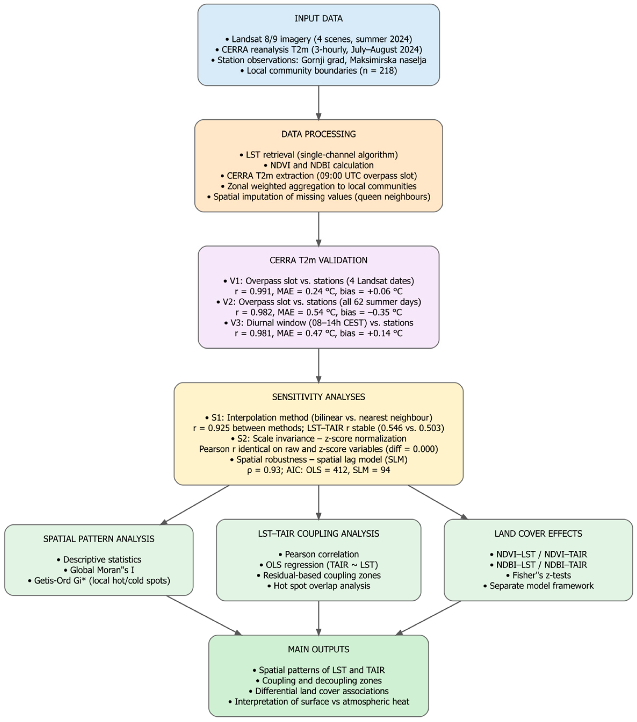
Figure 1. Methodological workflow of the study.
Atmosphere 17 00466 g001
Figure 2. Spatial distribution of (a) land surface temperature (LST) and (b) near-surface air temperature (TAIR) across Zagreb’s 218 local councils, summer 2024. (c) LST hot/cold spots and (d) TAIR hot/cold spots identified through Getis–Ord Gi* analysis (p < 0.05).
Atmosphere 17 00466 g002
Figure 3. Scatter plot of LST versus TAIR across 218 local councils, showing moderate positive correlation (r = 0.537, R2 = 0.288, p < 0.001), confirming H1 (partial coupling).
Atmosphere 17 00466 g003
Figure 4. Spatial distribution of coupling/decoupling zones based on TAIR~LST regression residuals.
Atmosphere 17 00466 g004
Figure 5. Hot/cold spot overlap map showing convergent zones (11.9% total).
Atmosphere 17 00466 g005
Figure 6. NDVI distribution across urban heat zone types in Zagreb (Summer 2024). (a) Spatial distribution; (b) NDVI by hot zone type; (c) LST–NDVI relationship with hot zone categories highlighted.
Atmosphere 17 00466 g006aAtmosphere 17 00466 g006b
Figure 7. Differential land cover associations. (a) NDVI, (b) NDBI.
Atmosphere 17 00466 g007
Table 1. Validation of CERRA T2m against station observations, Zagreb, summer 2024.
SchemePeriodNrMae (°C)Bias (°C)RMSE (°C)
V1: Overpass slot, 4 Landsat datesJuly–August 202480.9910.24+0.060.25
V2: Overpass slot, all summer daysJuly–August 20241240.9820.54−0.350.68
V3: Diurnal window (08–14 h CEST)July–August 20241240.9810.47+0.140.61
Table 2. Descriptive statistics for thermal and land cover variables across Zagreb’s 218 local councils, summer 2024.
VariableNMeanSDMinMedianMax
LST (°C)21837.853.7029.3838.5143.66
TAIR (°C)21829.150.7226.6829.3930.37
NDVI2180.550.160.230.540.83
NDBI218−0.090.06−0.22−0.080.04
Table 3. Global spatial autocorrelation (Moran’s I) for LST and TAIR.
ComponentMoran’s IExpected Ip Value
LST0.767−0.004<0.001
TAIR0.795−0.004<0.001
Table 4. Hot/cold spot classification frequency for LST and TAIR based on Getis–Ord Gi* analysis (p < 0.05, two-tailed).
ComponentCategoryCountPercent
LSTHot spot4219.26
LSTCold spot5022.93
LSTNot significant12657.79
TAIRHot spot2913.30
TAIRCold spot3315.14
TAIRNot significant15671.56
Table 5. Coupling zone classification based on regression residual magnitude.
Coupling TypeNPercent
Strong coupling10950.0
TAIR < expected5625.7
TAIR > expected5324.3
Table 6. Hot/cold spot overlap classification showing limited convergence and substantial divergence.
Overlap TypeNPercent
No significant pattern9543.6
LST hot only4118.8
TAIR hot only2812.8
Both cold2511.5
LST cold only209.2
TAIR cold only83.7
Both hot10.5
Table 7. Summary of differential land cover effects confirming H3.
IndexLST rLST CI LowerLST CI UpperTAIR rTAIR CI LowerTAIR CI UpperFisher zCohens qp_ValueConclusion
NDVI−0.970−0.977−0.961−0.478−0.574−0.36816.3411.576<0.001Confirmed
NDBI0.9730.9650.9790.4960.3890.59016.5831.599<0.001Confirmed
Table 8. Physical mechanisms contributing to spatial decoupling between LST and TAIR.
MechanismSpatial ScaleEffect on TAIRContribution to
Decoupling
Vertical turbulent mixing100 m–2 kmDisperses surface heat through boundary layer, diluting the surface thermal signalHigh
Horizontal advection5–50 kmImports non-local air masses, introducing TAIR patterns unrelated to local surface conditionsHigh
Residual temporal offsetInstantaneous~45 min mismatch between LST overpass (~09:45 UTC) and CERRA slot (09:00 UTC) during rapid morning heatingModerate
CERRA spatial resolution5.5 km native gridSmooths neighborhood-scale atmospheric gradients that local surface heterogeneity would otherwise produceModerate
Surface-atmosphere thermal lagMinutes–hoursSurface heats faster than overlying air, especially at midday under clear-sky conditionsModerate
Disclaimer/Publisher’s Note: The statements, opinions and data contained in all publications are solely those of the individual author(s) and contributor(s) and not of MDPI and/or the editor(s). MDPI and/or the editor(s) disclaim responsibility for any injury to people or property resulting from any ideas, methods, instructions or products referred to in the content.