Emergent Constraint on the Projection of Compound Dry and Hot Events in Guangdong Province by CMIP6 Models

Abstract

In the context of global warming, compound dry-hot events (CDHEs) are intensifying in Guangdong, yet CMIP6 projections remain uncertain. This study employs CMIP6 data and the Standardized Compound Event Indicator (SCEI) to quantify CDHEs severity, applying an observational constraint approach to reduce inter-model uncertainty. The results show that, after observational constraint, uncertainties decrease by about 63% and 77% in Period I and II under SSP126 and by about 57% and 59% under SSP585, greatly improving projection robustness. CDHE risk is highest in SSP585-Period II. Future dry-hot intensification in Guangdong generally increases from north to south, with western Guangdong most strongly affected. Although CDHEs weaken in other periods, western Guangdong shows persistent aggravation. Mechanism analyses indicate that SSP585-Period I is mainly linked to cold sea surface temperature (SST) anomalies in the South Atlantic and waters near Australia. After correction, dry-hot conditions show a marked weakening across Guangdong, although slight intensification persists over the Leizhou Peninsula. SSP585-Period II is primarily influenced by warm SST anomalies in the eastern Pacific and South Atlantic and cold anomalies in the North Pacific. The two SSP126 periods are associated with warm SST anomalies in the South Atlantic and waters near Australia and with cold anomalies in the South Atlantic, North Pacific, and North Atlantic, respectively. After correction, CDHEs generally weaken across Guangdong, although southern and south-central areas remain relatively severe. These findings indicate that historical key SST biases can strongly influence future CDHEs projections in Guangdong by modulating large-scale atmospheric circulation, including the Pacific-South American wave train, Indian Ocean SST anomalies, and the Western North Pacific Subtropical Anticyclone.

1. Introduction

In recent years, the increasing frequency of extreme weather and climate events, such as droughts, floods, heatwaves, and cold surges, has been closely linked to global climate change, posing serious threats to ecosystems and socioeconomic systems. Among these, drought and extreme heat are particularly destructive, exerting profound effects on agricultural production, water resource supply, energy supply, and human health [1,2,3]. When drought and extreme heat occur simultaneously or sequentially, their interactions significantly intensify the pressure on regional water resources, agriculture, industry, and ecosystems. Extreme heat accelerates potential evapotranspiration, aggravates soil moisture deficits, and enhances drought severity through an increased vapor pressure deficit. Conversely, such drought-induced soil moisture decline weakens evaporative cooling, enhances sensible heat flux, and elevates surface temperatures, thereby triggering or intensifying heatwaves [3,4,5]. The combined effects of extreme events pose much greater risks to ecosystem resilience and sustainable socioeconomic development than single events [1]. In recent decades, severe compound dry-hot events (CDHEs) have occurred frequently. For example, the 2003 European heatwave and 2010 Russian heatwave were both accompanied by severe drought, whereas the 2020 Australian bushfire season, driven by compound heat and drought, resulted in massive wildfires, economic losses, and ecological damage [6]. These events highlight the urgency and importance of advancing research on CDHEs.

Guangdong Province, located in southern China, is characterized by a subtropical monsoon climate, high population density, and intense economic activity. Its climate system is particularly sensitive to complex topography (e.g., the Nanling Mountains) and land-sea interactions. In the summer of 2022, Guangdong experienced an extreme compound hot-dry event lasting nearly two months, leading to water shortages for agricultural irrigation and record-breaking electricity demand in the Pearl River Delta [7]. This underscores the real-world significance of understanding future changes in CDHEs in the region.

Accurately simulating and projecting the evolution of CDHEs provides the scientific basis for climate adaptation strategies. Climate system models are the core tools for simulating and projecting climate variability and change, enabling us to understand past mechanisms and anticipate future changes under different emission scenarios [8,9]. Phase 6 of the Coupled Model Intercomparison Project (CMIP6) has been widely applied in global and regional studies of CDHEs. At the global scale, Petrova et al. [10] used CMIP6 and CMIP5 models together with land aridity duration (LAD) index; however, future CDHE frequencies may be underestimated, with constrained projections showing an extension of the global mean LAD by 10 days. Yao et al. [11] revealed through CMIP6 multi-model ensembles that precipitation trends are the primary control on future CDHEs, and that under high-emission scenarios, constrained projections show a 9.68–18.74% lower frequency than the original estimates. At the regional scale, Bole et al. [12] constructed an emergent constraint framework using CMIP6 models and GPCP precipitation data over the Mongolian Plateau and found that constrained estimates reduced uncertainty in drought intensity and frequency by 30–40%. Chen et al. [13], focusing on China, applied emergent constraint methods to correct warm biases in CMIP6, reducing projected extreme heat intensity by 0.63 °C and the affected population share by 15% compared to unconstrained projections.

However, multi-model ensemble simulations still contain systematic errors. Internal variability, differences in physical processes, and parameterization schemes lead to substantial uncertainties that limit the reliability of extreme event projections [14]. Globally, inter-model differences are the primary source of uncertainty in compound hot-dry event projections across 66% of the global land areas [15].

To reduce these uncertainties, emergent constraint methods have gained increasing attention in climate modeling. By integrating long-term high-quality observations, this approach quantifies and corrects model biases, thereby improving projection accuracy [16,17]. Compared with traditional bias correction methods, it is better suited for capturing the nonlinear responses of compound events [18]. This method has been applied to reduce the uncertainties in various climate extremes, including temperature [19], precipitation [20], and drought [12].

Similarly, substantial uncertainties remain in CMIP6 projections of compound dry-hot events (CDHEs) over Guangdong. As the economic core region of southern China, Guangdong has experienced frequent CDHEs in recent years, and its climate risks have pronounced socioeconomic impacts. Therefore, improving the reliability of future regional projections is an urgent priority. Unlike previous observational constraint studies that mainly focused on circulation indices or regional mean climate variables, this study is oriented toward regional disaster risk assessment and uses the compound dry-hot risk indicator (ΔSCEI) over Guangdong as the constraint target. By identifying key SST modes that drive inter-model discrepancies and applying observational constraints, we aim to enhance projection reliability. This study addresses two core scientific questions: (1) Why do CMIP6 models exhibit significant biases and inter-model inconsistencies in simulating CDHEs (ΔSCEI) over Guangdong? What are the dominant uncertainty modes, and which key SST patterns regulate them? (2) Can observational constraints establish quantitative relationships between key SST patterns and future model performance, thereby reducing projection uncertainties across different emission scenarios and periods while clarifying the associated circulation mechanisms? To address these questions, we analyze historical and future climate variables from 22 CMIP6 models and construct constraint relationships based on reanalysis data to correct future projections. By further diagnosing atmospheric circulation and moisture transport processes, we reveal the physical pathways through which key SST patterns influence Guangdong CDHEs via wave-train propagation and anomalous western North Pacific circulation, thereby improving the credibility of regional climate risk assessments.

2. Data and Methods

2.1. Data

2.1.1. CMIP6 Data

This study employed monthly mean near-surface air temperature (tas), precipitation (pr), sea surface temperature (tos), zonal (ua) and meridional (va) winds at 850 hPa, sea-level pressure (psl), and geopotential height at 500 hPa (zg) from 22 CMIP6 models (

Table 1. Basic Information on 22 CMIP6 global climate models.

Number	Model	Institution/Country	Latitude × Longitude	Approximate Resolution (°)
1	ACCESS-CM2	CSIRO/Australia	144 × 192	1.25 × 1.88
2	ACCESS-ESM1-5	CSIRO/Australia	145 × 192	1.24 × 1.88
3	AWI-CM-1-1-MR	AWI/Germany	192 × 384	0.94 × 0.94
4	BCC-CSM2-MR	BCC-CMA/China	160 × 320	1.13 × 1.13
5	CAMS-CSM1-0	CAMS/China	160 × 320	1.13 × 1.13
6	CanESM5-1	CCCMA/Canada	64 × 128	2.81 × 2.81
7	CanESM5	CCCMA/Canada	64 × 128	2.81 × 2.81
8	CAS-ESM2-0	CAMS/China	64 × 128	2.81 × 2.81
9	CESM2-WACCM	NCAR/USA	192 × 288	0.94 × 1.25
10	CMCC-CM2-SR5	CMCC/Italy	192 × 288	0.94 × 1.25
11	CMCC-ESM2	CMCC/Italy	192 × 288	0.94 × 1.25
12	FGOALS-g3	LASG-IAP/China	90 × 180	2.00 × 2.00
13	FIO-ESM-2-0	FIO-QLNM/China	192 × 288	0.94 × 1.25
14	IITM-ESM	CCCR-IITM/India	94 × 192	1.91 × 1.88
15	MIROC6	MIROC/Japan	128 × 256	1.41 × 1.41
16	MPI-ESM1-2-HR	MPI-M/Germany	192 × 384	0.94 × 0.94
17	MPI-ESM1-2-LR	MPI-M/Germany	96 × 192	1.88 × 1.88
18	MRI-ESM2-0	MRI/Japan	160 × 320	1.13 × 1.13
19	NESM3	NUIST/China	96 × 192	1.88 × 1.88
20	NOrESM2-LM	NCC/Norway	96 × 144	1.88 × 2.50
21	NOrESM2-MM	NCC/Norway	192 × 288	0.94 × 1.25
22	TaiESM1	AS-RCEC/Taiwan	192 × 288	0.94 × 1.25

). In the following sections, the model numbers correspond to the sequences listed in Table 1. The analysis focused on the seasonal mean characteristics and their changes during the boreal warm season (May-October). The experiments included the historical simulation and future projections under the Shared Socioeconomic Pathways SSP1-2.6 and SSP5-8.5 (hereafter referred to as SSP126 and SSP585, respectively). The historical simulations cover 54 years (1961–2014), whereas the future projections span 75 years (2025–2099). In line with China’s national strategy of carbon peaking and carbon neutrality, particularly the core goal of striving to achieve carbon neutrality around 2060, the future period was further divided into two stages: 2025–2059 (Period I) and 2060–2099 (Period II). This division is consistent with both the needs of national socioeconomic development research and the conventions of climate statistical analysis. The multi-model ensemble (MME) was calculated as the mean of 22 models with equal weights. A single ensemble member (r1i1p1f1) was used for each model. All variables were interpolated to a common 1° × 1° grid using the bilinear interpolation method in Climate Data Operators (CDO; cdo remapbil), ensuring consistent spatial resolution and providing a basis for subsequent multivariable analysis.

2.1.2. Reanalysis Data

The reanalysis data were derived from the European Centre for Medium-Range Weather Forecasts Reanalysis Version 5 (ERA5) [21], including monthly mean temperature and precipitation at a spatial resolution of 0.25° × 0.25°. Sea surface temperature (SST) data were obtained from ERA5 (0.25° × 0.25°) and ERSSTv5 [22] (2° × 2°). The observation period spans 1961–2014. To ensure consistency and facilitate direct comparison with the CMIP6 model outputs, all observational variables were bilinearly interpolated to a common 1° × 1° grid.

2.1.3. Study Area

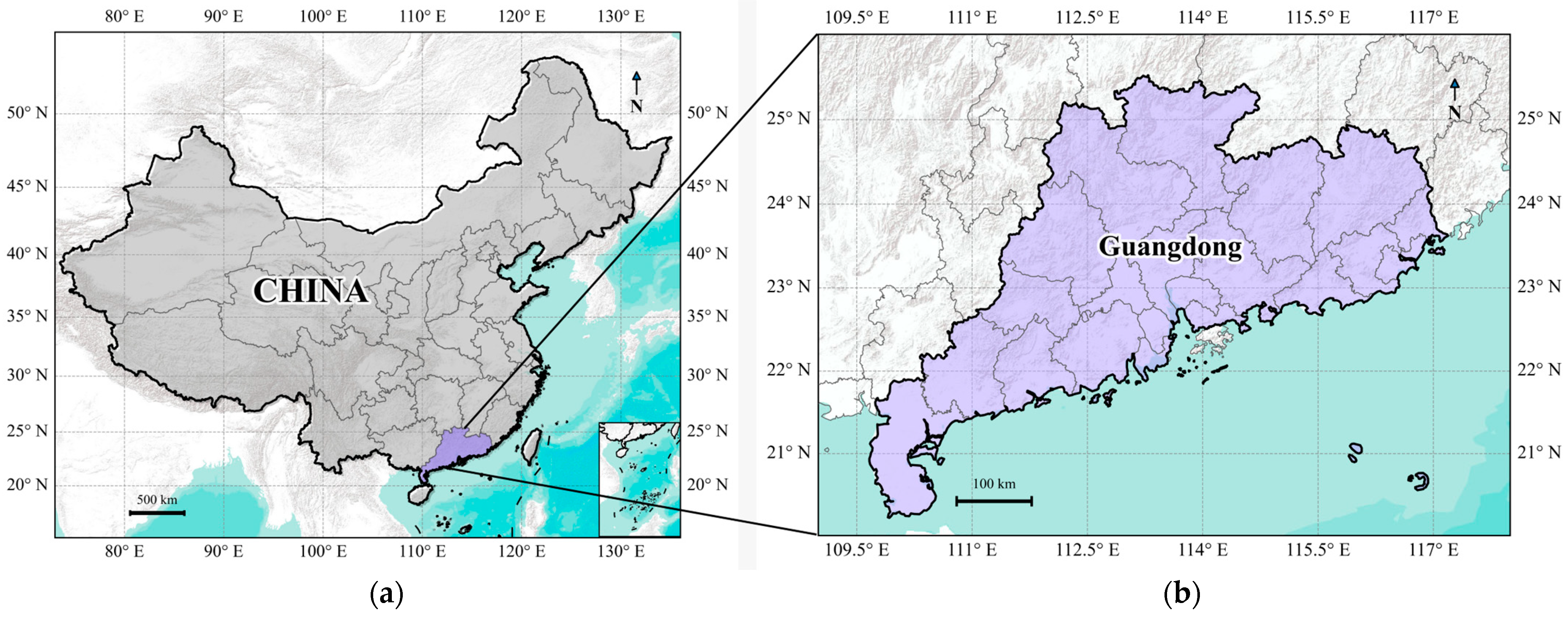
The study area in Figure 1 is Guangdong Province, China (20–26° N, 109–118° E). Located in the coastal region of South China, Guangdong is strongly influenced by the East Asian monsoon and is characterized by a typical subtropical climate. The regional climate exhibits pronounced spatial heterogeneity due to the combined effects of the Nanling Mountains as a topographic barrier and land-sea interactions. The climate system in this region is highly sensitive to both natural variability and anthropogenic influences.

2.2. Methods

2.2.1. Index Definition

Based on monthly mean temperature and monthly accumulated precipitation during 1961–2014, this study calculated the Standardized Temperature Index (STI) [23] and the Standardized Precipitation Index (SPI) [24] to characterize hot events and meteorological drought events, respectively. A copula-based joint index, the Standardized Compound Event Indicator (SCEI) [25], was developed using STI and SPI to quantify the severity of CDHEs. In this study, only the SCEI values from May to October (the warm season) were used for subsequent analyses. Negative SCEI values indicate a tendency toward compound dry-hot conditions, and lower SCEI values indicate greater severity of compound dry-hot conditions.

To calculate the SCEI, the time series of SPI and STI were first transformed into empirical marginal distribution functions, $\mathrm{u}=\mathrm{P}\left(\mathrm{X}\le \mathrm{x}\right) \mathrm{a}\mathrm{n}\mathrm{d} \mathrm{v}=\mathrm{P}(\mathrm{Y}\le \mathrm{y}),$ using the Gringorten plotting position formula $\mathrm{F}({\mathrm{X}}_{\mathrm{i}})={\displaystyle \frac{\mathrm{i}-0.44}{\mathrm{n}+0.12}}$ [26]. These empirical probabilities were then mapped into the standard normal space through the inverse standard normal transformation ${\mathsf{\Phi }}^{-1}$. Subsequently, the Gaussian copula (Equation (1)) was employed to characterize the dependence structure between SPI and STI, and the joint probability of high-temperature events occurring under drought conditions was derived from the copula-based joint distribution. Finally, the joint probabilities (Equation (2)) were standardized by reapplying the Gringorten formula and standard normal transformation, yielding the SCEI (Equation (3)).

$$\mathrm{C}(\mathrm{u},\mathrm{v})={\mathsf{\Phi }}_2({\mathsf{\Phi }}^{-1}(\mathrm{u}),{\mathsf{\Phi }}^{-1}(\mathrm{v});\mathsf{\rho }),$$

(1)

$$\mathrm{p}=\mathrm{u}-\mathrm{C}(\mathrm{u},\mathrm{v}),$$

(2)

$$\mathrm{S}\mathrm{C}\mathrm{E}\mathrm{I}={\mathsf{\Phi }}^{-1}(\mathrm{F}(\mathrm{p})),$$

(3)

where ${\mathsf{\Phi }}^{-1 }$ is the inverse of the standard normal distribution, $\mathsf{\rho }$ is the Pearson correlation coefficient between SPI and STI, and ${\mathsf{\Phi }}_2$ is the bivariate standard normal cumulative distribution function (CDF).

The Copula function is introduced to construct the joint distribution of two random variables and to estimate the probability of their simultaneous occurrence (or joint exceedance of thresholds). Common Copula functions are generally classified into two major categories: Elliptical Copulas (e.g., Gaussian and t) and Archimedean Copulas (e.g., Frank, Clayton, and Gumbel) [27]. For modeling the joint distribution of STI and SPI, four widely used Copula functions, Gaussian, Frank, Clayton, and Gumbel, were selected for comparative fitting. The Akaike Information Criterion (AIC) [28] was employed to evaluate the goodness of fit of each function, with smaller AIC values indicating better performance. Based on the AIC, the AIC values of the four Copula types were calculated for each grid cell across Guangdong Province for all 22 CMIP6 models. The Copula with the minimum AIC at each grid cell was identified as the optimal Copula for that location. The proportion of grid cells where each Copula was selected as optimal was then calculated for each model, and the Copula with the highest proportion was determined as the optimal Copula for that model (

Table 2. Optimal Copula functions for the 22 global climate models (historical simulations).

Number	Model	Gaussian	Clayton	Gumbel	Frank	Best Copula
1	ACCESS-CM2	9	3	0	3	gaussian
2	ACCESS-ESM1-5	15	0	0	0	gaussian
3	AWI-CM-1-1-MR	6	8	0	1	clayton
4	BCC-CSM2-MR	8	0	0	7	gaussian
5	CAMS-CSM1-0	13	0	0	2	gaussian
6	CanESM5-1	15	0	0	0	gaussian
7	CanESM5	15	0	0	0	gaussian
8	CAS-ESM2-0	13	0	0	2	gaussian
9	CESM2-WACCM	15	0	0	0	gaussian
10	CMCC-CM2-SR5	2	0	0	13	frank
11	CMCC-ESM2	8	5	0	2	gaussian
12	FGOALS-g3	5	10	0	0	clayton
13	FIO-ESM-2-0	13	0	0	2	gaussian
14	IITM-ESM	11	0	0	4	gaussian
15	MIROC6	15	0	0	0	gaussian
16	MPI-ESM1-2-HR	15	0	0	0	gaussian
17	MPI-ESM1-2-LR	15	0	0	0	gaussian
18	MRI-ESM2-0	5	3	0	7	frank
19	NESM3	11	0	0	4	gaussian
20	NOrESM2-LM	4	11	0	0	clayton
21	NOrESM2-MM	15	0	0	0	gaussian
22	TaiESM1	3	4	0	8	frank

). Finally, among the optimal Copulas identified across the 22 models, the Gaussian Copula, which had the highest overall frequency, was selected as the globally optimal model and was uniformly applied to the subsequent joint probability analyses for all models.

2.2.2. Inter-Model Empirical Orthogonal Function (EOF) Analysis

In this study, the conventional empirical orthogonal function (EOF) decomposition method was first applied to identify and extract the dominant modes of uncertainty in projected SCEI changes over Guangdong. Specifically, an inter-model EOF decomposition was performed on the multi-model ensemble of projected SCEI change fields:

$$∆\mathrm{S}\mathrm{C}\mathrm{E}\mathrm{I}\prime (\mathrm{m},\mathrm{s})\cong {\sum }_{\mathrm{i}=1}^{\mathrm{n}}(\mathrm{P}{\mathrm{C}}_{\mathrm{i},\mathrm{m}}\times {\mathrm{E}\mathrm{O}\mathrm{F}}_{\mathrm{i},\mathrm{s}}),$$

(4)

where ∆SCEI denotes the projected change in SCEI over Guangdong, defined as the future change relative to the historical period (1961–2014). To facilitate interpretation of the severity of compound dry-hot events, the sign of ∆SCEI was reversed; thus, ∆SCEI > 0 indicates intensification of events, while ∆SCEI < 0 indicates mitigation. Here, m represents the model index, s denotes the spatial grid, n is the EOF mode number, and the prime symbol indicates deviations from the multi-model ensemble mean. The EOF decomposition helps identify the most representative modes of inter-model variability, providing a basis for subsequent constraint analyses.

2.2.3. Constrained Index

Based on the principal components (PCs) extracted from inter-model empirical orthogonal function (EOF) analysis, potential constraint relationships were established to link the inter-model differences in the historical period with future projection outcomes. These relationships were used to constrain the uncertainty metrics of future climate projections, referred to as constrained indices (IDs).

$$\mathrm{I}\mathrm{D}(\mathrm{m},\mathrm{i})={\mathrm{S}\mathrm{S}\mathrm{T}}_{\mathrm{h}\mathrm{i}\mathrm{s}\mathrm{t}}(\mathrm{m},\mathrm{i})\cdot {\mathrm{S}\mathrm{S}\mathrm{T}\prime }_{\mathrm{P}\mathrm{C}}(\mathrm{m},\mathrm{i}),$$

(5)

Here, $\mathrm{m}$ denotes the model index, and i represents the PC mode index. ${\mathrm{S}\mathrm{S}\mathrm{T}}_{\mathrm{h}\mathrm{i}\mathrm{s}\mathrm{t}}$ refers to the historically simulated mean SST of the ith mode from the mth model within the constrained region, whereas ${\mathrm{S}\mathrm{S}\mathrm{T}}_{\mathrm{P}\mathrm{C}}^{\prime }$ denotes the regression coefficient of ${\mathrm{S}\mathrm{S}\mathrm{T}}_{\mathrm{h}\mathrm{i}\mathrm{s}\mathrm{t}}$ onto the corresponding PC mode.

2.2.4. Emergent Constraint Method

A statistical relationship was established between the future projected change Y (i.e., PCs) and the historical constrained index X (i.e., IDs; Equation (5)) to constrain the multi-model ensemble results. Based on these 22 models, a linear regression model was constructed between Y and X, as follows:

$$\mathrm{Y}=\overline{\mathrm{Y}}+\mathrm{r}(\mathrm{X}-\overline{\mathrm{X}}),$$

(6)

where $\mathrm{r} = {\displaystyle \frac{{\mathsf{\sigma }}_{\mathrm{Y}}}{{\mathsf{\sigma }}_{\mathrm{x}}}}\mathsf{\rho }$ is the correlation coefficient and $\mathsf{\rho }$ is the regression coefficient. $\overline{\mathrm{Y}}$ and $\overline{\mathrm{X}}$ denote the multimodel means, and ${\mathsf{\sigma }}_{\mathrm{Y}}$ and ${\mathsf{\sigma }}_{\mathrm{x}}$ represent the inter-model standard deviations of PCs and IDs, respectively. In this formulation, $\overline{\mathrm{Y}}$ = 0 and ${\mathsf{\sigma }}_{\mathrm{Y}}$ = 1.

To incorporate the observational uncertainty into the constraint, this study used an additive noise model under the Gaussian assumption. Observations ${\mathrm{X}}_{\mathrm{o}\mathrm{b}\mathrm{s}}$ were related to historical simulations to estimate the Signal-to-noise ratio ($\mathrm{SNR}={\mathsf{\sigma }}_{\mathrm{model}}^2/{\mathsf{\sigma }}_{\mathrm{obs}}^2$), which was then used to adjust the regression coefficient $\mathsf{\rho }$. When the SNR ≫ 1, the effect of this correction was negligible.

After correcting $\mathsf{\rho }$, the constrained linear regression model can be expressed as

$$\overline{{\mathrm{Y}}_{\mathrm{C}}}=\overline{\mathrm{Y}}+{\displaystyle \frac{\mathsf{\rho }}{1+{\mathrm{S}\mathrm{N}\mathrm{R}}^{-1}}}(\overline{{\mathrm{X}}_{\mathrm{o}\mathrm{b}\mathrm{s}}}-\overline{\mathrm{X}}),$$

(7)

and the corresponding inter-model variance is

$${\mathsf{\sigma }}_{{\mathrm{Y}}_{\mathrm{C}}}^2=(1-{\displaystyle \frac{{\mathrm{r}}^2}{1+{\mathrm{S}\mathrm{N}\mathrm{R}}^{-1}}}){\mathsf{\sigma }}_{\mathrm{Y}}^2,$$

(8)

The relative variance reduction and the total variance reduction due to the constraint are:

$$∆{\mathsf{\sigma }}_{\mathrm{C}}^2(\mathrm{i})=(1-{\displaystyle \frac{{\mathsf{\sigma }}_{{\mathrm{Y}}_{\mathrm{C}}}^2(\mathrm{i})}{{\mathsf{\sigma }}_{\mathrm{Y}}^2}})={\displaystyle \frac{{\mathrm{r}}^2(\mathrm{i})}{1+{\mathrm{S}\mathrm{N}\mathrm{R}}^{-1}(\mathrm{i})}},$$

(9)

$${∆\mathsf{\sigma }}_{\mathrm{total}}^2={\mathrm{w}}_1\times ∆{\mathsf{\sigma }}_{\mathrm{P}\mathrm{C}1}^2+{\mathrm{w}}_2\times ∆{\mathsf{\sigma }}_{\mathrm{P}\mathrm{C}2}^2,$$

(10)

where i is the number of PC modes index. The total variance reduction is calculated as a weighted sum based on the variance contribution of each PC, and ${\mathrm{w}}_1$ and ${\mathrm{w}}_2$ represent the variance contributions of PC1 and PC2, respectively.

2.2.5. Constrained Projections of CDHE Changes

Once the constrained principal components (${\mathrm{P}\mathrm{C}}_{\mathrm{C}}$) are obtained, future SCEI projections are revised and re-estimated using EOF-based linear reconstruction:

$$∆{\mathrm{S}\mathrm{C}\mathrm{E}\mathrm{I}}_{\mathrm{C}}=∆\stackrel{\mathrm{—}}{\mathrm{SCEI}}+{∆\mathrm{SCEI}\prime }_{\mathrm{C}} \cong ∆\stackrel{\mathrm{—}}{\mathrm{SCEI}}+{\sum }_{\mathrm{i}=1}^{\mathrm{n}}({\mathrm{PC}}_{\mathrm{C}}(\mathrm{i})\times {\mathrm{E}\mathrm{O}\mathrm{F}}_{\mathrm{s}}(\mathrm{i})),$$

(11)

where the subscript “C” denotes the constrained result and the overbar represents the multi-model mean from CMIP6.

3. Results

3.1. Uncertainties in Inter-Model Spread

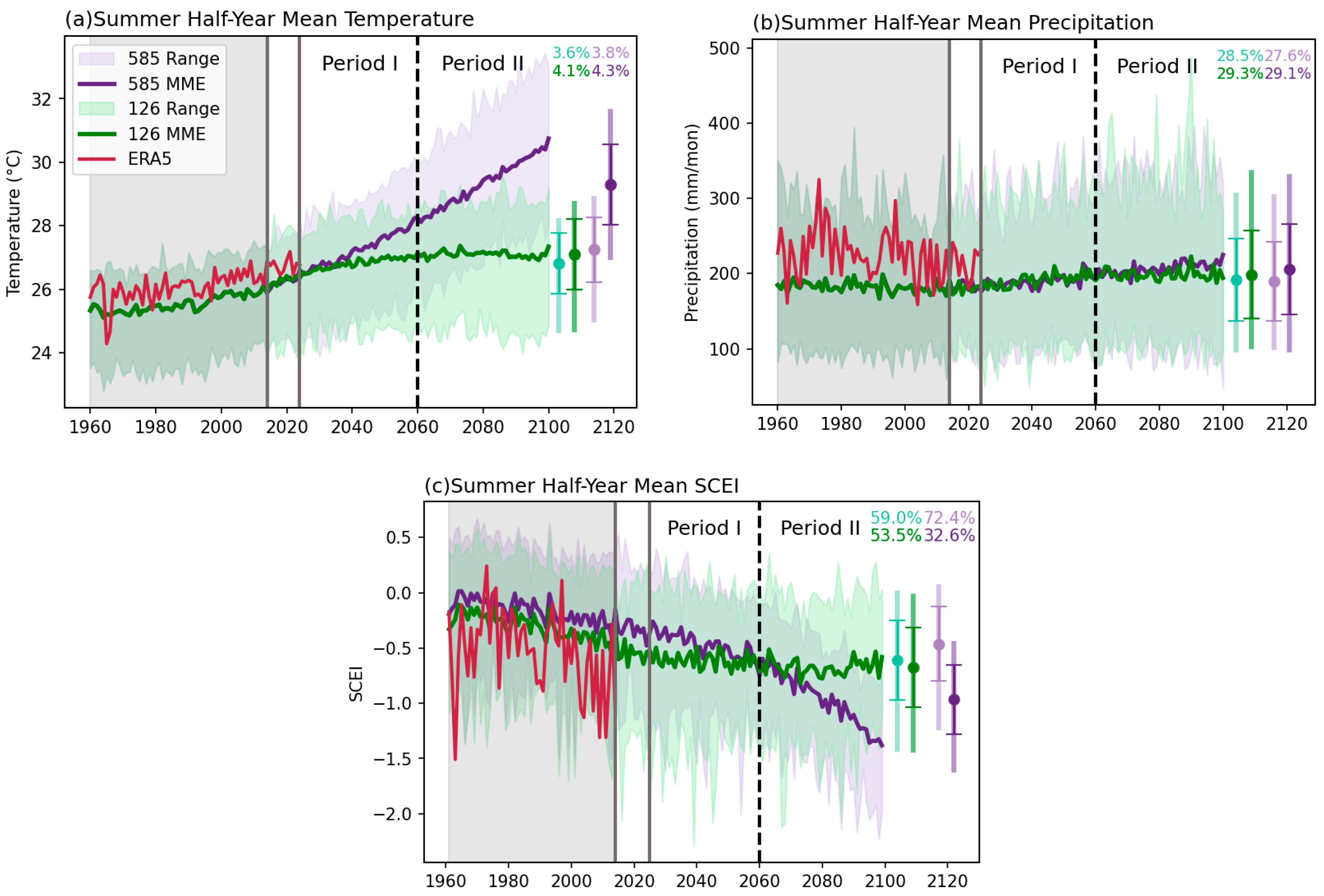
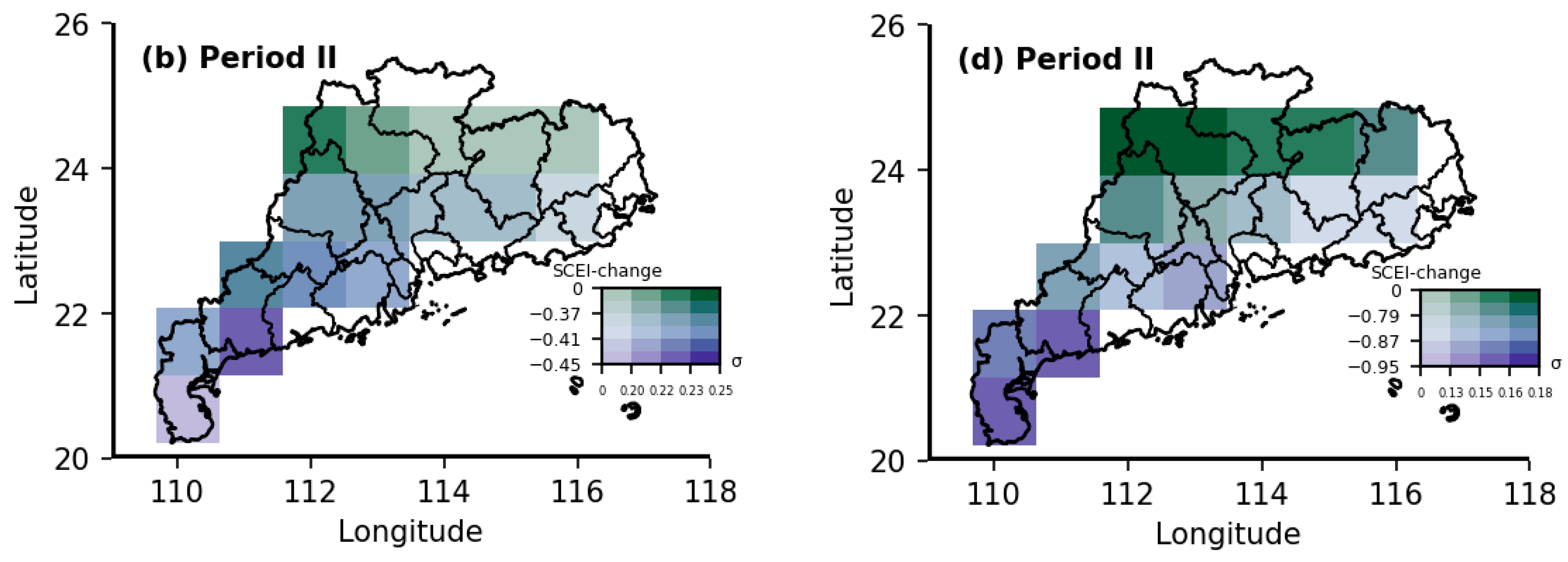
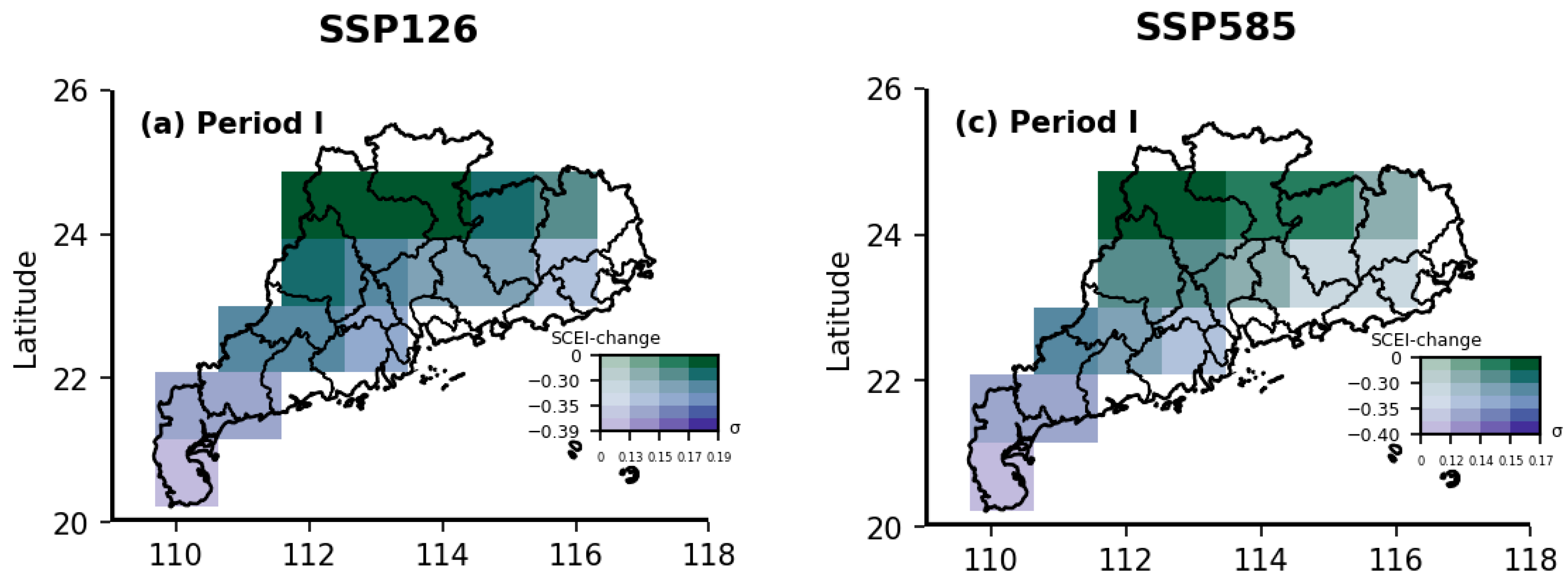
Many studies have indicated that under different emission scenarios, such as the low-emission SSP1-2.6 and high-emission SSP5-8.5 pathways, CMIP6 models exhibit varying degrees of inter-model spread in projections of future climate change. This uncertainty is reflected in the projected frequency of CDHEs, drought duration, and the evolution of key circulation systems, such as the subtropical high. For some indicators, inter-model dispersion is large, and opposite signs of future change have been suggested, indicating that model uncertainty remains a major limitation in the reliable projection of extreme climate events [10,11,29]. Accordingly, this study focuses on both SSP126 and SSP585 scenarios and finds that CMIP6 projections of CDHEs over Guangdong also show pronounced inter-model differences under different emission pathways. Before the 2020s, the reanalysis data and the MME showed relatively consistent temperature changes, remaining around 25–27 °C. After the 2020s, with ongoing climate warming, temperatures exhibited a continuous increasing trend. Under SSP585, temperatures are projected to rise to approximately 31 °C by 2099, whereas under SSP126 the maximum temperature remains below 28 °C (Figure 2a). In contrast, precipitation showed smaller variations. Although a slight increase is projected during Period II, its overall trend is less pronounced than that of temperature, and the increasing trend under SSP585 is slightly stronger than that under SSP126 (Figure 2b). Despite the relatively small changes in precipitation, the SCEI exhibits a significant decreasing trend, indicating that the severity of CDHEs intensifies markedly over time (Figure 2c). This intensification is more pronounced in southern Guangdong (Figure 3), with stronger increases under SSP585 than SSP126, and larger changes in Period II compared to Period I. The error bars on the right side of Figure 2 represent the coefficients of variation (CV) for the two periods under SSP126 and SSP585, which are used to quantify model uncertainty. The results indicate that substantial uncertainty remains in future projections. The CV of temperature is smaller than that of precipitation, suggesting relatively lower inter-model spread for temperature; however, both variables exhibit considerable uncertainty, which is greater in Period II than in Period I. Moreover, inter-model uncertainty in temperature is higher under SSP585 than SSP126, while precipitation uncertainty is slightly lower under SSP585 (Figure 2a,b). Uncertainty in future SCEI projections is even higher. However, when comparing different periods, inter-model uncertainty is lower in Period II (Figure 2c). Under SSP126, uncertainty differences between the two periods are small, whereas under SSP585, uncertainty varies markedly between periods, with the lowest uncertainty occurring in Period II. Spatially, inter-model uncertainty is generally higher in northern Guangdong than in southern Guangdong, except during SSP585 Period II, when relatively high uncertainty is observed in both northern and western Guangdong (Figure 3).

3.2. Leading Modes of Inter-Model Spread Uncertainties

To reveal the sources of model uncertainty, we performed inter-model EOF analyses of projected SCEI changes for two periods under both the SSP585 and SSP126 scenarios.

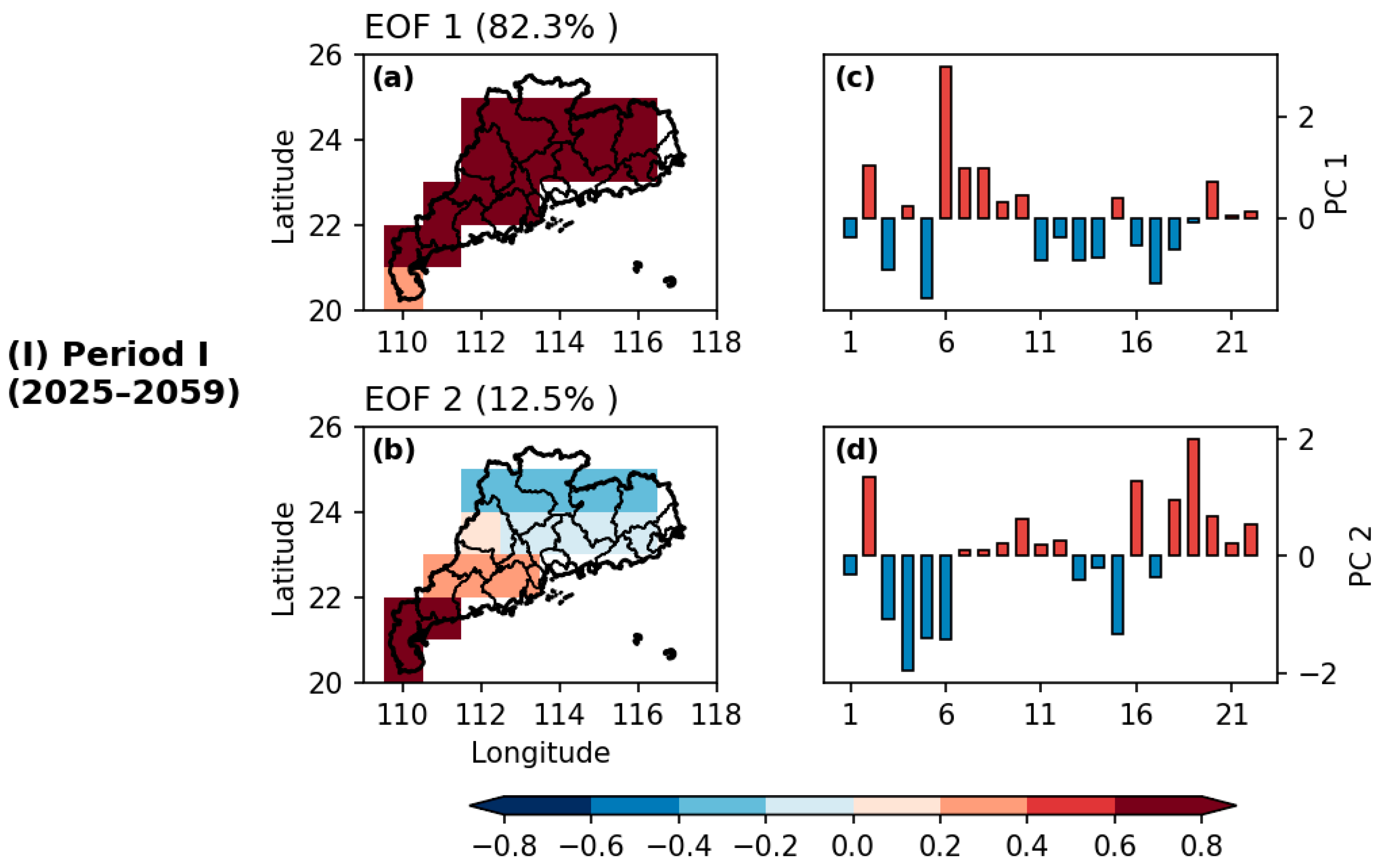
Under SSP585, the first two leading principal components (PC1 and PC2) explain nearly 95% of the total inter-model variance in Period I and more than 95% in Period II (Figure 4). The EOF1 spatial patterns in both periods exhibit a monopole structure: positive anomalies in Period I and negative anomalies in Period II. In Period I, loadings over the Leizhou Peninsula are relatively smaller than those in other regions. EOF1 accounts for 82.3% and 84.0% of the inter-model variance in Period I and Period II, respectively. EOF2 displays a dipole pattern. In Period I, positive anomalies dominate southern Guangdong while negative anomalies occur in the north, with a gradual transition from south to north, explaining 12.5% of the variance. In Period II, the spatial pattern is opposite to that of Period I, explaining 11.8% of the variance.

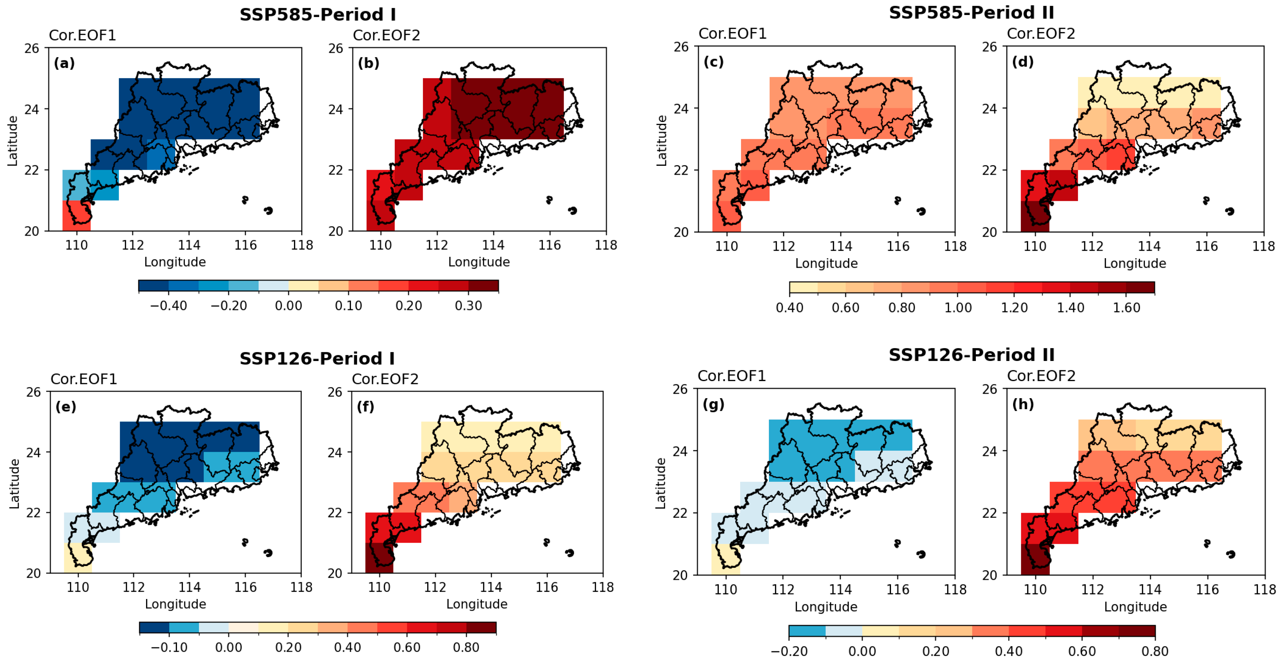
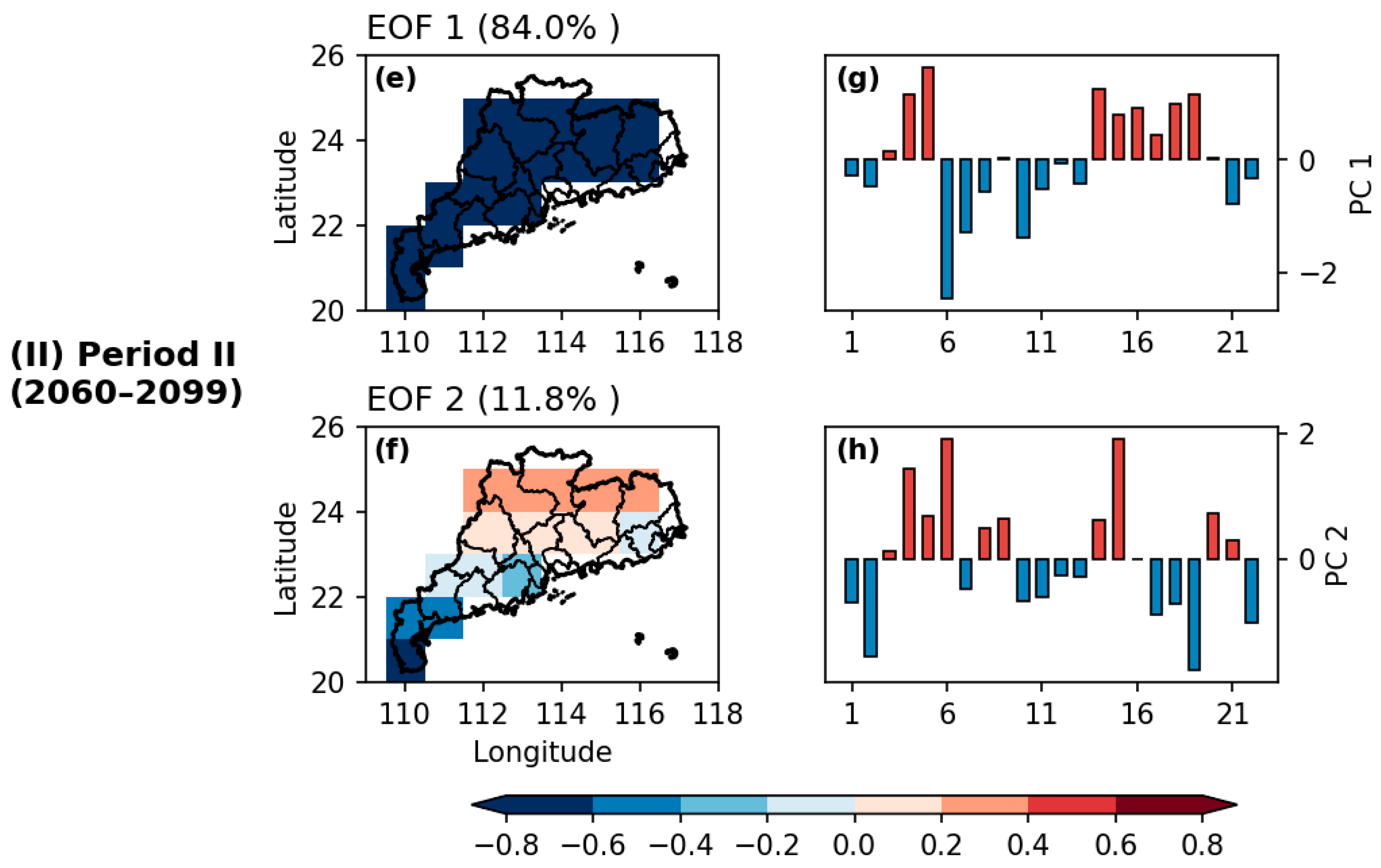
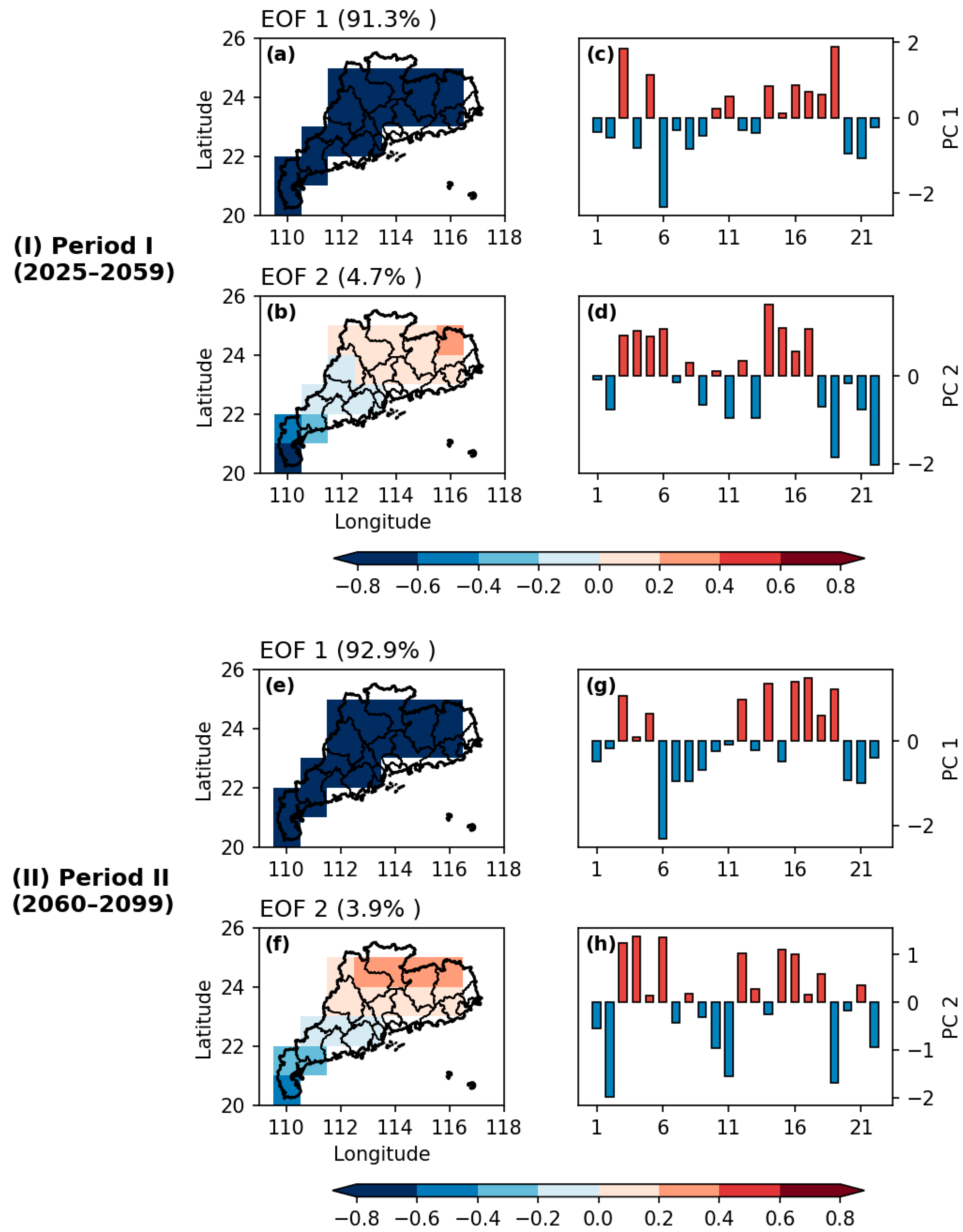
Under SSP126 (Figure 5), the spatial characteristics are generally consistent between the two periods. EOF1 exhibits a monopole structure with negative anomalies in both periods. EOF2 shows a dipole pattern characterized by positive anomalies in the north and negative anomalies in the south, with a gradual transition from northeast to southwest. In Period II, positive anomalies over northern Guangdong are more pronounced than in Period I, whereas negative anomalies over the Leizhou Peninsula are stronger in Period I. For both periods, the first two leading components explain more than 95% of the total inter-model variance.

Because these two dominant modes capture a substantial portion of the total variance, applying observational constraints to their PCs can potentially reduce uncertainty in SCEI projections.

3.3. Historical SST Patterns Related to the Uncertainty Modes

The subtropical high-pressure circulation is the primary and most direct factor influencing compound dry-hot events, and its position and intensity are strongly modulated by sea surface temperature (SST) anomalies [30]. To identify the appropriate constraint indices, we regressed the historical mean SST fields (1961–2014) from each model’s historical simulation onto inter-model standardized principal components (PCs). This approach allowed us to determine the specific oceanic regions and associated SST variability modes that effectively indicate biases in the projected SCEI changes, thereby leading to the construction of two constraint indices: ID1 and ID2.

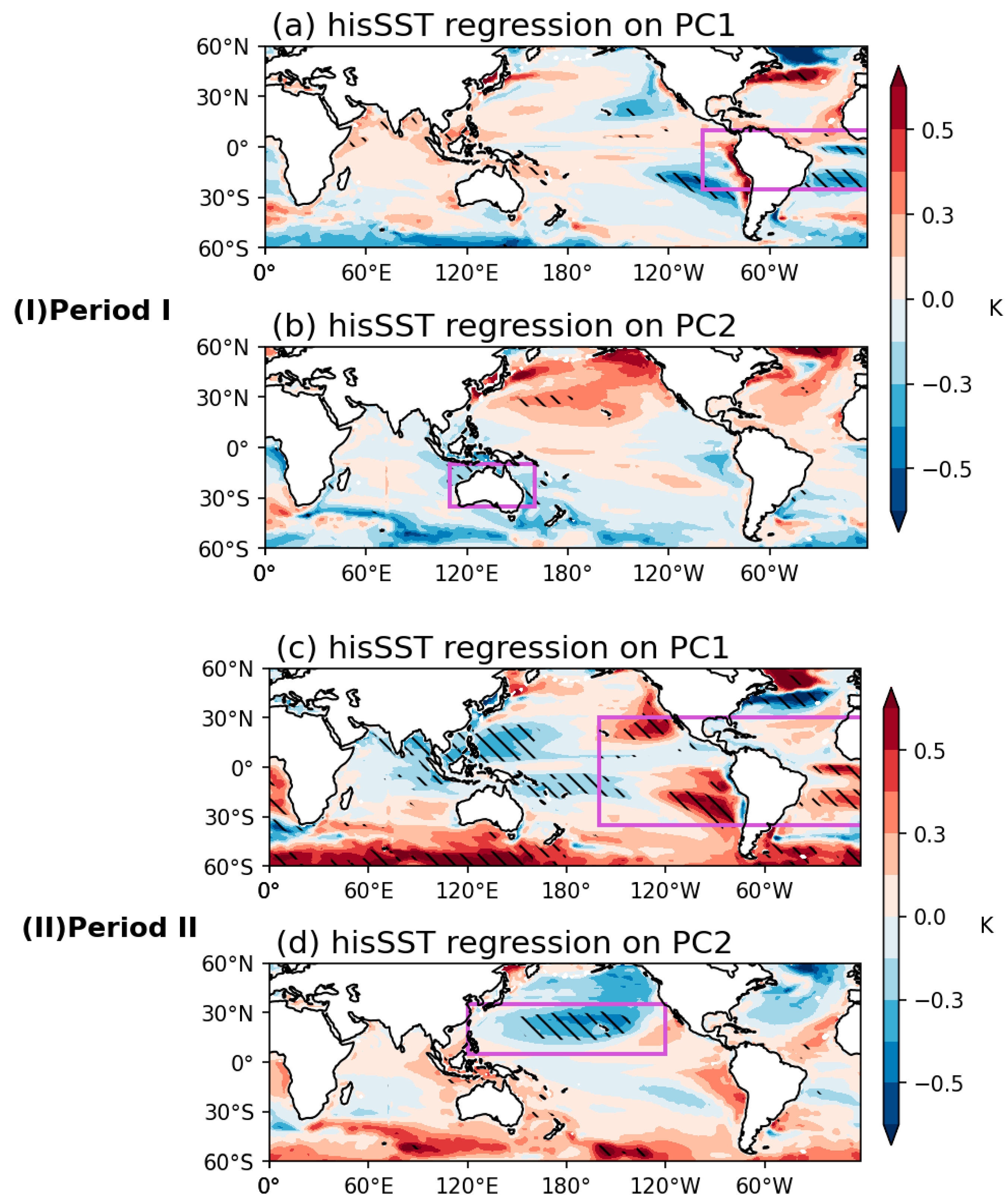
Under the SSP585 scenario, the first leading mode in Period I was associated with historical SST anomalies in the South Atlantic (25° S-10° N, 100° W-0°; Figure 6a). This indicates that when a model simulates colder historical SSTs over the South Atlantic, the projected future SCEI changes are more likely to exhibit positive anomalies, implying intensified compound dry-hot conditions across most of Guangdong Province. The second leading mode was mainly related to SST anomalies in the waters surrounding Australia (10°–35° S, 110–160° E; Figure 6b). When a model simulates warmer historical SST biases in this region, the projected SCEI changes show a spatial pattern characterized by positive anomalies in southern Guangdong and negative anomalies in the north, indicating aggravated compound dry-hot conditions in the south and relative weakening in the north.

In Period II, the SST-related regions of the first leading mode were similar to those in Period I but covered a broader area (Figure 6). This mode was associated with SST anomalies in the eastern Pacific and South Atlantic (35° S-30° N, 160° W-0°; Figure 6c). When models simulate warmer historical SSTs over the subtropical eastern Pacific and South Atlantic, future SCEI changes tend to exhibit more pronounced negative anomalies, suggesting a general weakening of compound dry-hot conditions across most of Guangdong. The second leading mode was mainly influenced by SST anomalies in the North Pacific (5–35° N, 120° E-120° W; Figure 6d). When models simulate colder historical SSTs in the North Pacific, future SCEI changes are more likely to show positive anomalies in northern Guangdong, indicating intensified compound dry-hot events, while negative anomalies dominate in the south, suggesting relative mitigation.

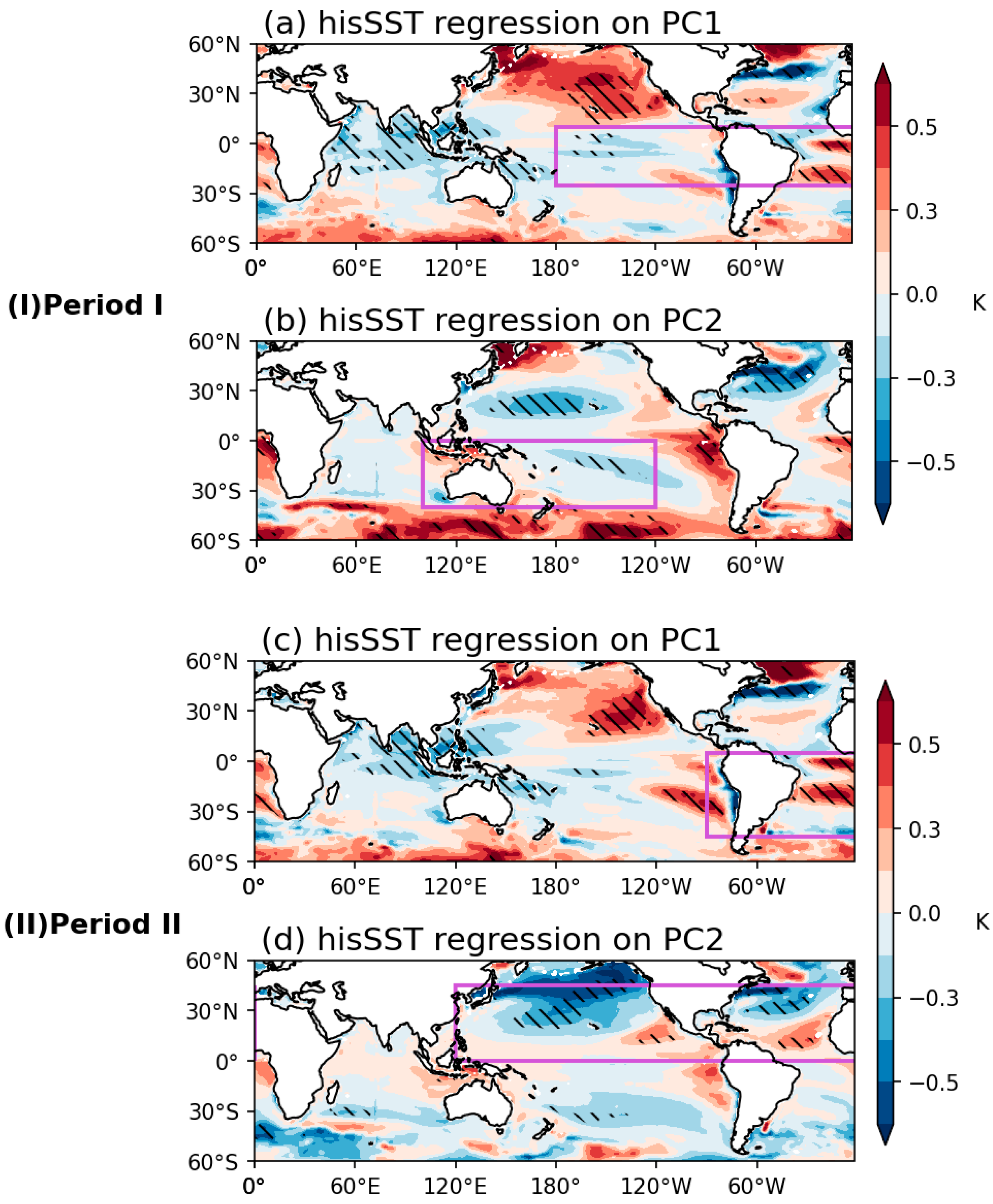
Under the SSP126 scenario, although the spatial patterns of the dominant modes of inter-model uncertainty were generally consistent between the two periods, the SST anomaly patterns and key regions responsible for these uncertainties differed (Figure 7). For Period I, the key SST anomaly regions of the first leading mode were similar to those under SSP585 but additionally included the central equatorial Pacific (25° S-10° N, 180–0°; Figure 7a). When historical SSTs were warmer in the South Atlantic and colder in the central equatorial Pacific, projected SCEI changes tended to show more pronounced negative anomalies, implying weakened compound dry-hot conditions across most of Guangdong. The second leading mode was similar to that of SSP585 Period I but additionally included the South Pacific region, covering the waters near Australia and the broader South Pacific (40° S-0°, 100° E-120° W; Figure 7b). When models simulated warmer SSTs near Australia and colder SSTs in the South Pacific, future SCEI changes tended to exhibit positive anomalies in northern Guangdong, indicating aggravated compound dry-hot events, while negative anomalies dominated in the south, indicating relative weakening.

For Period II, the key SST anomaly regions of the first leading mode were nearly identical to those of the first mode under SSP585 Period I (45° S-5° N, 90° W-0°; Figure 7c). Warmer historical SSTs in the South Atlantic were associated with more pronounced negative SCEI anomalies in future projections, suggesting weakened compound dry-hot conditions across most of Guangdong. The second leading mode was also similar to that under SSP585 Period II but included additional influence from the North Atlantic, in addition to the North Pacific (0–45° N, 120° E-0°; Figure 7d). When historical SSTs were colder in both the North Pacific and North Atlantic, projected SCEI changes displayed a dipole pattern with positive anomalies in the north and negative anomalies in the south, indicating aggravated compound dry-hot conditions in northern Guangdong and weakened conditions in the south.

3.4. Constraining PC Uncertainty Using Observational SST Patterns

After establishing the relationships between SST patterns and leading modes of inter-model spread, two constrained indices (ID1 and ID2) were constructed for each period under both scenarios. Using relatively reliable SST observations (ERSSTv5 and ERA5), these indices were employed to apply emergent constraints to projected SCEI changes. Each model’s historical mean-state SST was projected onto two SST modes associated with the dominant inter-model leading principal components (PCs), providing a measure of each model’s fidelity in reproducing the observed climate during the historical period (see Methods). This formed an observationally constrained framework for each period, enabling the effective correction of future projections of CDHEs over Guangdong.

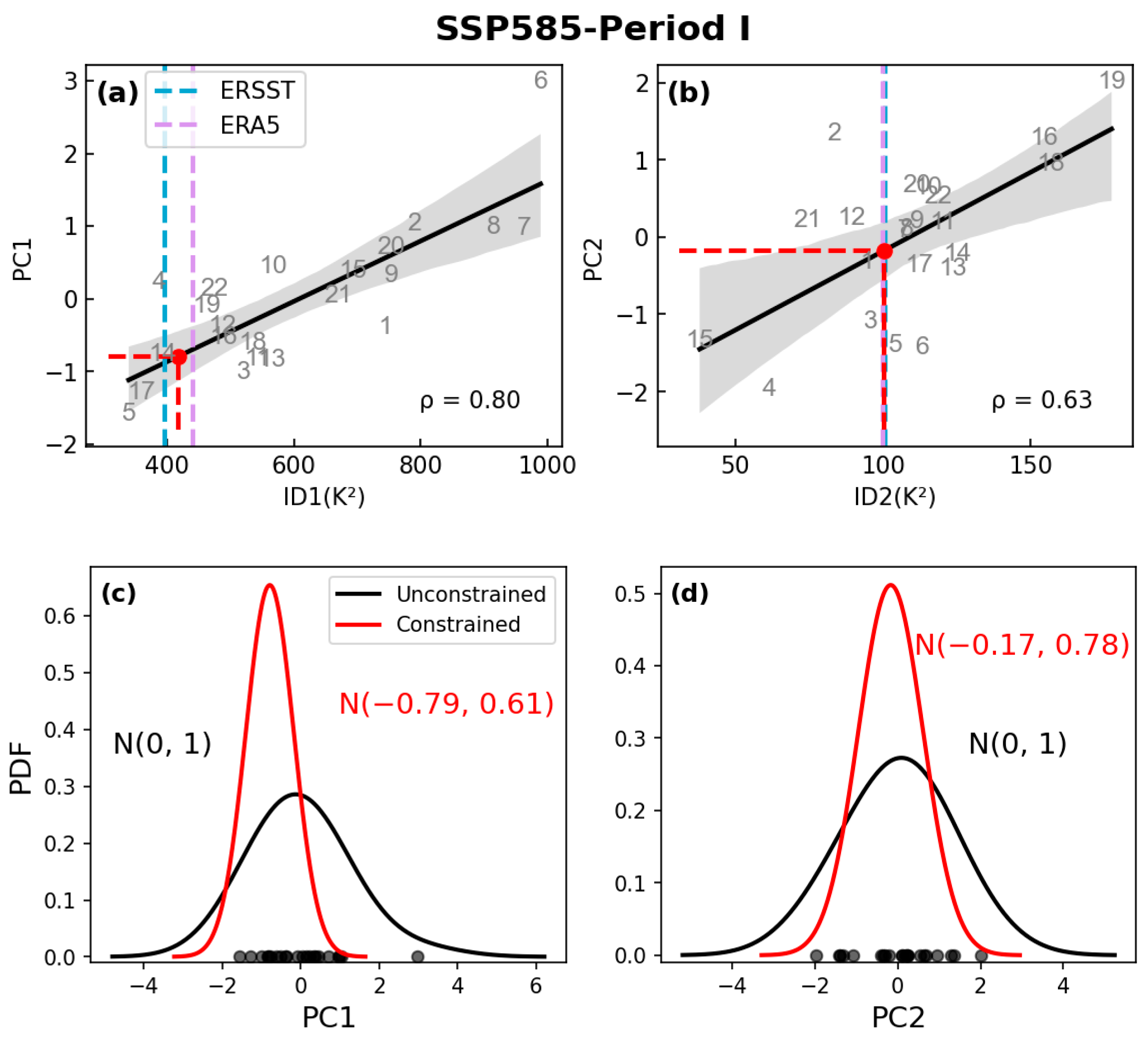
Under the SSP585 scenario, the observational constraint relationships in the two periods were generally similar. For the Period I constraint relationship (Figure 8), ID1 represents the South Atlantic region in the Southern Hemisphere. Approximately 81% of the models show ID1 values higher than the observations, indicating that most models simulated colder SSTs in this region. ID2 corresponds to the waters surrounding Australia, where about 68% of the models exhibit ID2 values higher than the observations, suggesting that more than half of the models simulated colder SSTs than observed in this region. Based on the correlations and observed SST pattern indices (IDs), the principal components (PCs) can be estimated and their variances reduced. Due to the use of observational data to constrain future projections, observational uncertainties must be taken into account. Under the Gaussian assumption with an additive noise model, historical SSTs are used to link observations with model simulations, and the signal-to-noise ratio (SNR; see Section 2.2.4) is calculated. The SNR values for ID1 and ID2 are (6.4)² and (60)², respectively. When SNR ≫ 1, the influence of the correction becomes negligible. A high SNR indicates that the observational signal is much stronger than the noise, implying strong consistency and a stable statistical relationship between observations and model simulations. Incorporating observational information into the constraint therefore effectively improves the reliability of the constrained projections. The variances of PC1 and PC2 were reduced by approximately 63% and 39%, respectively. Considering that PC1 and PC2 explained 82.3% and 12.5% of the total variance, respectively (see Figure 4), the overall reduction in explained variance of PC1 and PC2 (include here the percentage of the total variance explained by PC1 + PC2) achieved through the emergent constraint was estimated at approximately 57% (63% × 82.3% + 39% × 12.5%) (see Equation (10)). The constrained values of PC1 and PC2 are −0.79 ± 0.61 and −0.17 ± 0.78 (mean ± 1σ), respectively (Figure 8c,d). These results indicate that, after correction, both PC1 and PC2 tend to shift toward negative values (out-of-phase behavior). By correcting the cold SST biases in the South Atlantic and the waters surrounding Australia, the intensities of the EOF1 and EOF2 spatial modes are weakened, respectively.

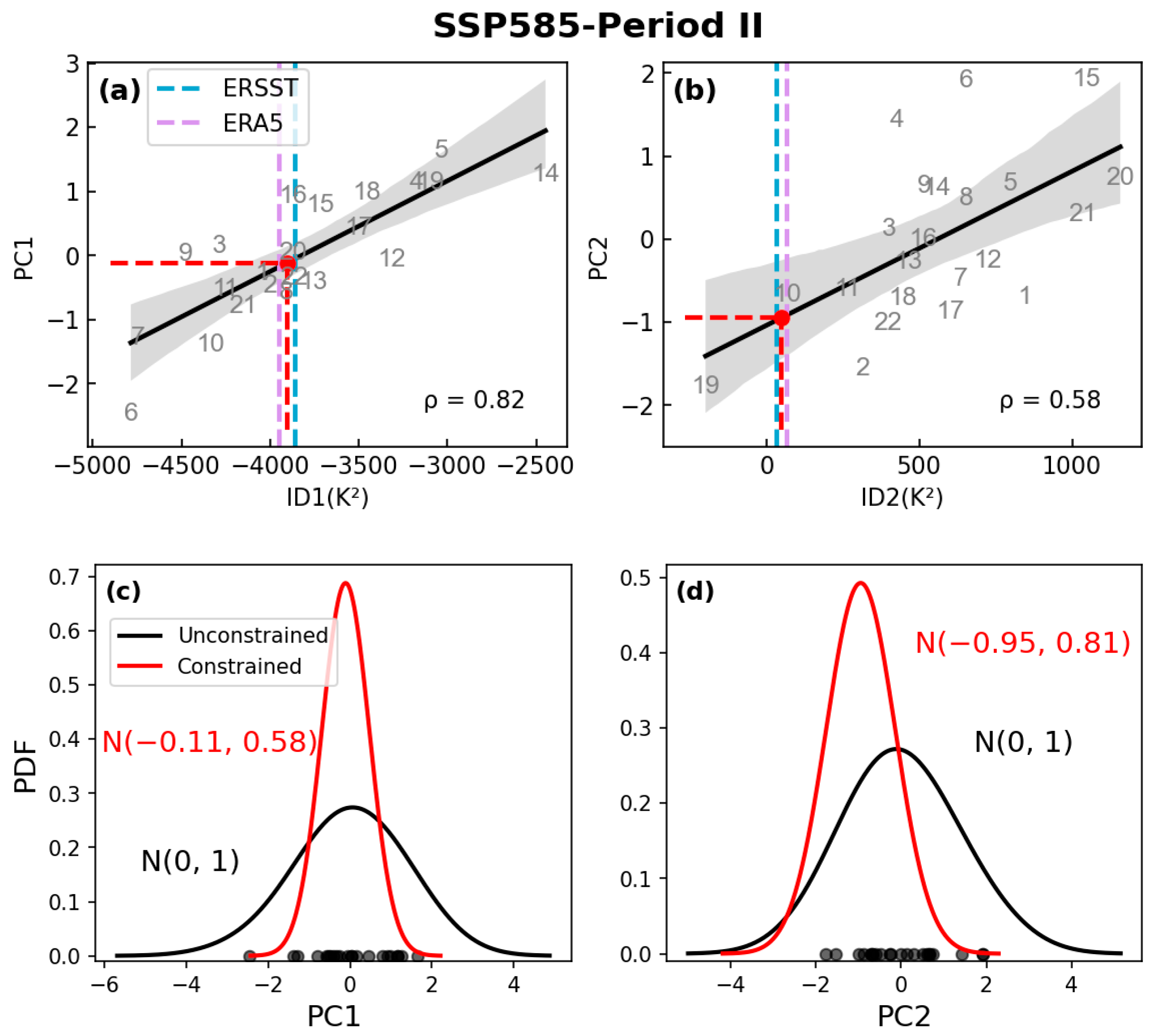
For the Period II constraint relationship (Figure 9), ID1 represents the eastern Pacific and South Atlantic regions. Nearly 60% of the models show ID1 values higher than the observations, indicating that more than half of the models simulated warmer SSTs in these regions. ID2 corresponds to the North Pacific, where about 95% of the models show ID2 values higher than the observations, suggesting that nearly all models simulated colder SSTs in this region. For ID1 and ID2, the SNR is (9.4)² and (12.7)², respectively. The variances of PC1 (84%) and PC2 (11.8%) were reduced by approximately 66% and 34%, respectively, resulting in an overall variance reduction of approximately 59% (66% × 84% + 34% × 11.8%) (see Equation (10)). The constrained values of PC1 and PC2 are −0.11 ± 0.58 and −0.95 ± 0.81, respectively (Figure 9c,d). As in Period I, both PC1 and PC2 tend to shift toward negative values after correction (out-of-phase behavior). By correcting the warm SST biases in the eastern Pacific and South Atlantic and the cold SST bias in the North Pacific, the intensities of the EOF1 and EOF2 spatial modes are weakened, respectively.

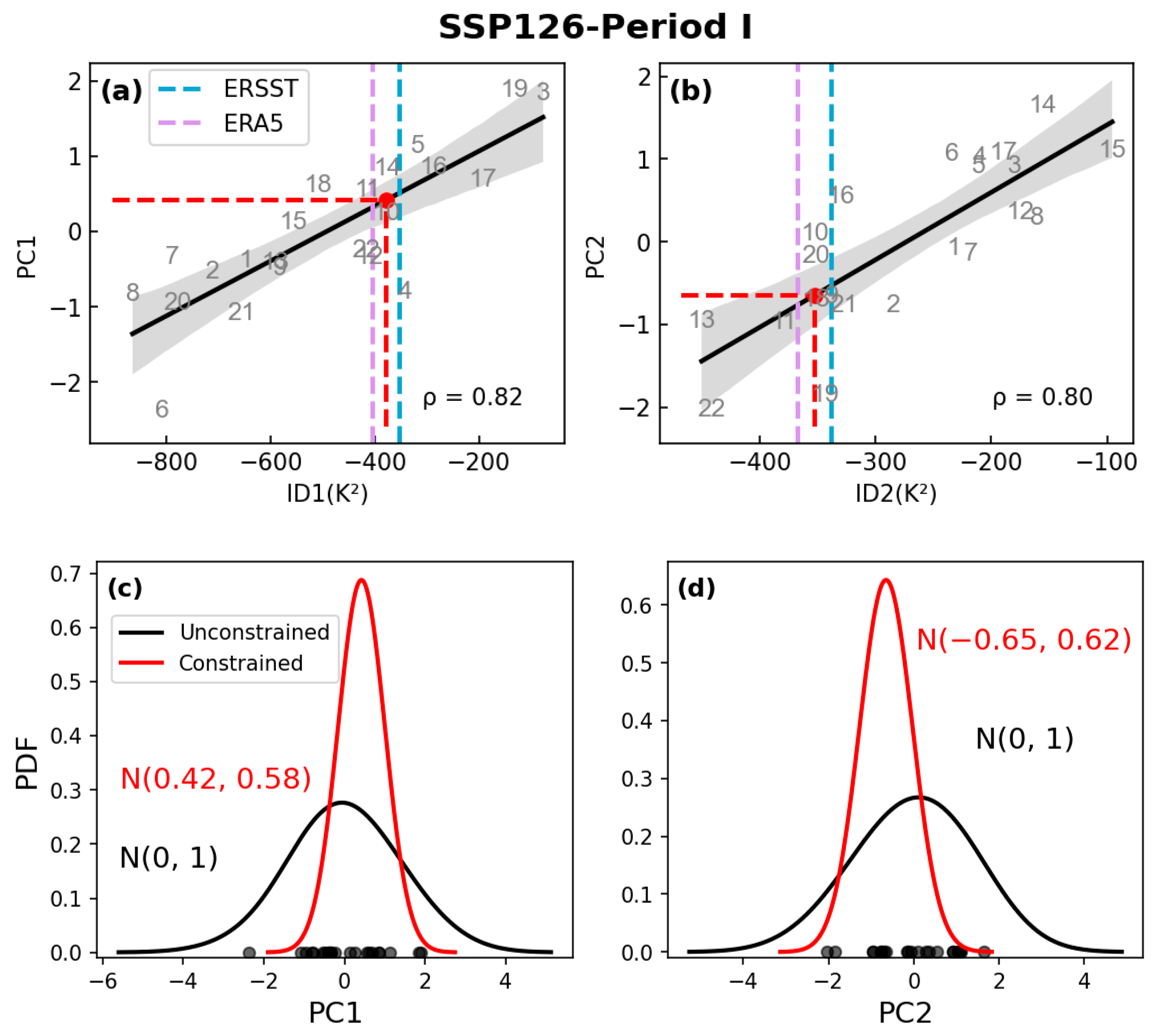
Under the SSP126 scenario, for the Period I constraint relationship (Figure 10), ID1 mainly represents the South Atlantic and central-eastern Pacific regions. About 64% of the models show ID1 values lower than the observations, indicating that more than half of the models simulated colder historical SSTs in the South Atlantic and warmer historical SSTs in the central equatorial Pacific. ID2 corresponds to the waters surrounding Australia and the South Pacific region. Approximately 72% of the models show ID2 values higher than the observations, suggesting that, relative to the observations, most models simulated warmer historical SSTs near Australia and colder historical SSTs in the South Pacific. For ID1 and ID2, the SNR is (6.2)² and (4.7)², respectively. After observational constraint, the variances of PC1 (91.3%) and PC2 (4.7%) were reduced by approximately 66% and 61%, respectively, with an overall variance reduction of approximately 63% (66% × 91.3% + 61% × 4.7%) (see Equation (10)). The constrained values of PC1 and PC2 are 0.42 ± 0.58 and −0.65 ± 0.62 (mean ± 1σ), respectively (Figure 10c,d). These results indicate that, after correction, PC1 tends to shift toward positive values (in-phase behavior), and by correcting the cold SST bias in the South Atlantic and the warm SST bias in the central equatorial Pacific, the intensity of the EOF1 spatial mode is enhanced. In contrast, PC2 tends to shift toward negative values (out-of-phase behavior), and by correcting the warm SST bias in the waters surrounding Australia and the cold SST bias in the South Pacific, the intensity of the EOF2 spatial mode is weakened.

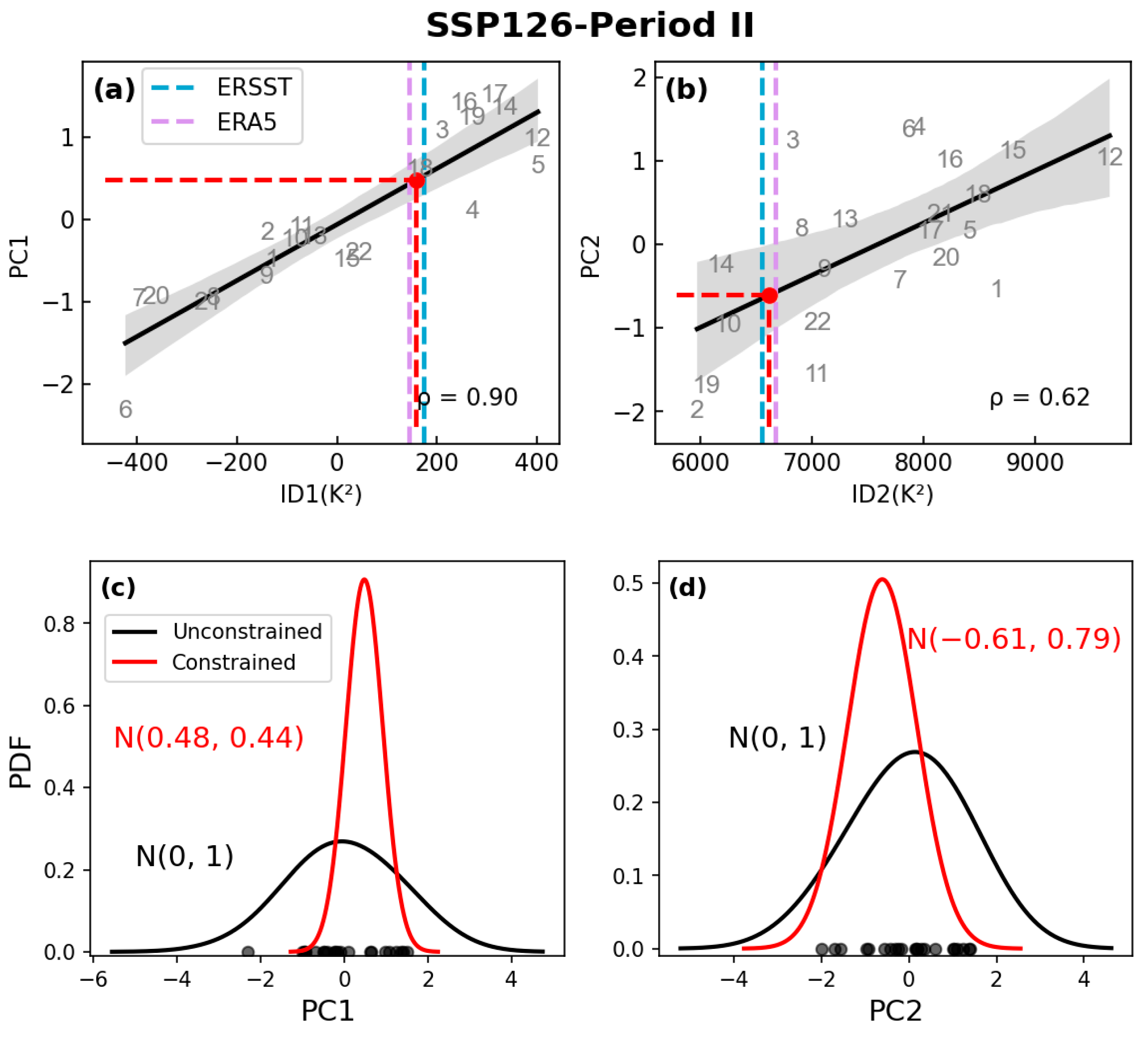
For the Period II constraint relationship (Figure 11), ID1 mainly represents the South Atlantic region. About 60% of the models show ID1 values lower than the observations, indicating that more than half of the models simulated colder historical SSTs in this region. ID2 corresponds to the North Pacific and North Atlantic regions. Approximately 81% of the models show ID2 values higher than the observations, suggesting that most models simulated colder historical SSTs in these regions. For ID1 and ID2, the SNR is (12.9)² and (11.8)², respectively. The variances of PC1 (92.9%) and PC2 (3.9%) were reduced by approximately 81% and 38%, respectively, resulting in an overall variance reduction of approximately 77% (81% × 92.9% + 38% × 3.9%) (see Equation (10)). The constrained values of PC1 and PC2 are 0.48 ± 0.44 and −0.61 ± 0.79 (mean ± 1σ), respectively (Figure 11c,d). These results indicate that, after correction, PC1 tends to shift toward positive values (in-phase behavior), and by correcting the cold SST bias in the South Atlantic, the intensity of the EOF1 spatial mode is enhanced. In contrast, PC2 tends to shift toward negative values (out-of-phase behavior), and by correcting the cold SST biases in the North Pacific and North Atlantic, the intensity of the EOF2 spatial mode is weakened.

3.5. Before and After the Emergent Constraints

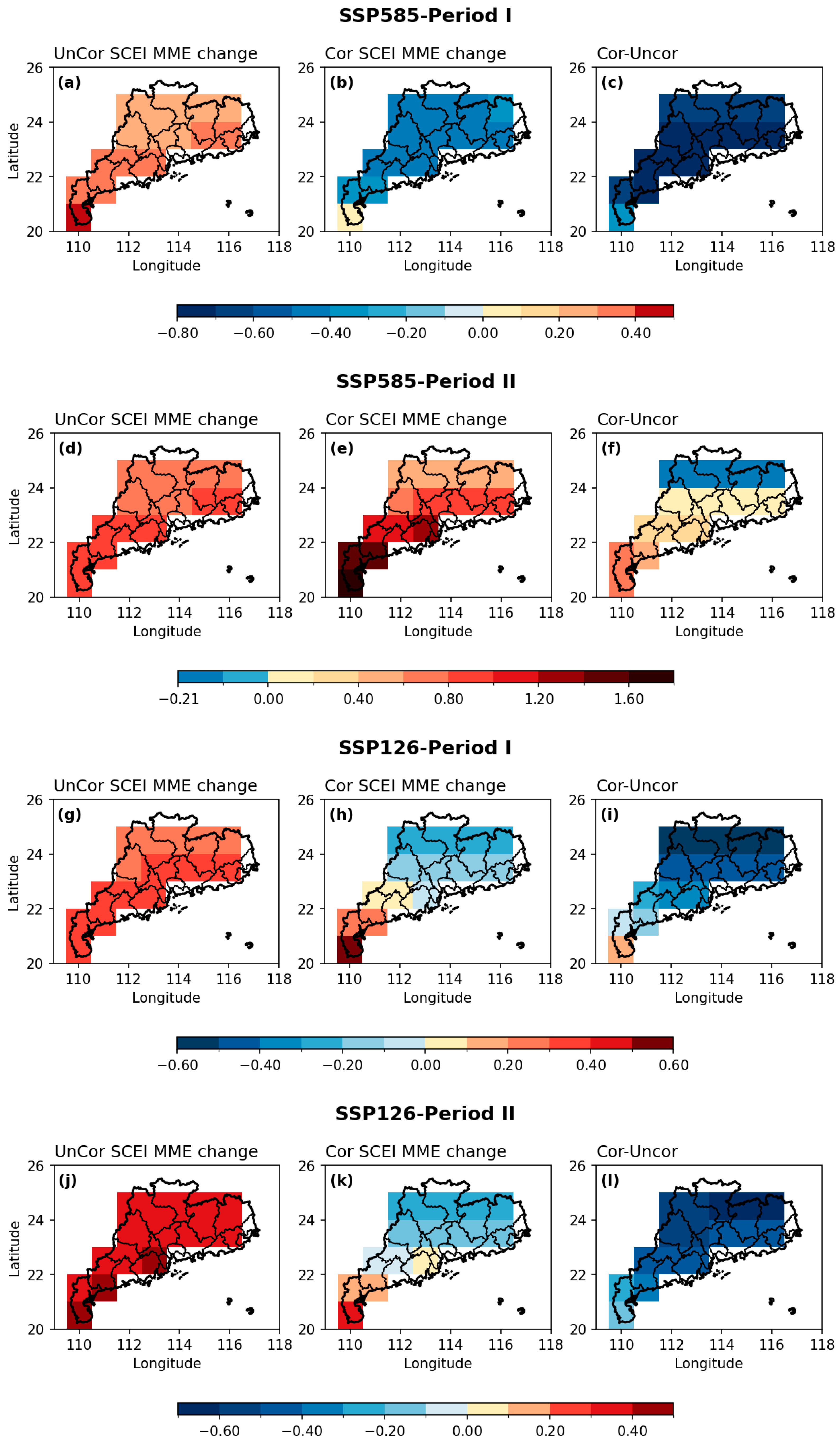
After determining the optimal PCs based on the constraint relationships, the spatial distribution of the projected SCEI was further reconstructed. The constrained projections show that, during Period I under SSP585 (relative to the historical period), SCEI changes are negative across most of Guangdong Province, with positive values confined to the Leizhou Peninsula. This indicates that compound dry-hot events generally weaken across the province except over the Leizhou Peninsula (Figure 12b). In contrast, the unconstrained projections suggest an overall intensification of events during this period, with the most severe conditions occurring in western Guangdong. After applying the observational constraint, corrections are generally larger over central and northern Guangdong and weakest over western Guangdong (Figure 12c). In terms of modal contributions, SCEI changes over most of the province are primarily constrained by EOF1 (Figure 13a), which exhibits a pronounced north-south gradient ranging from −0.50 to 0.16. By comparison, EOF2 (Figure 13b) shows a weaker north-south gradient, with values ranging from 0.24 to 0.34.

During Period II under SSP585, constrained projections indicate an overall intensification of compound dry-hot events across Guangdong, with positive SCEI changes throughout the province. The positive anomalies increase from north to south, indicating a spatial pattern characterized by weaker impacts in the north and stronger impacts in the south, with western Guangdong being most prominent (Figure 12e). Without observational constraint, the entire province exhibits a nearly uniform intensification. After correction, dry-hot conditions weaken markedly in northern Guangdong but intensify significantly in western Guangdong, forming a spatial gradient that transitions from weakening in the north to intensification in the south (Figure 12f). Modal contribution analysis further indicates that SCEI changes during this period are mainly constrained by EOF2 across most regions of Guangdong (Figure 13c,d).

Under SSP126, the spatial characteristics of Period I are generally similar to those under SSP585. Constrained projections show that compound dry-hot events weaken across most of the province, except in western Guangdong (including the Leizhou Peninsula, with a broader affected area than under SSP585). A north-to-south transition is evident, shifting gradually from weakening to intensification, and the projected severity of future compound dry-hot events is greater in southern Guangdong (Figure 12h). Before applying the observational constraint, the original model simulations also indicate an overall intensification of dry-hot events, with more severe conditions in the central-southern regions than in the central-northern regions. After correction, intensification becomes more pronounced in western Guangdong and is stronger than that under SSP585, while most other regions exhibit weakened dry-hot conditions compared with the unconstrained results. Only the Leizhou Peninsula shows enhanced intensification after correction (Figure 12i). Further modal contribution analysis indicates that SCEI changes in northern Guangdong are mainly constrained by EOF1, whereas those in southern Guangdong are primarily constrained by EOF2 (Figure 13e–f).

Period II under SSP126 shows spatial features similar to those in Period I. The main difference is that, before constraint, projections indicate nearly uniform intensification of compound dry-hot events across the province. After applying the observational constraint, dry-hot conditions weaken across most regions except western Guangdong. However, the severity in central and southern Guangdong is lower than that in Period I (Figure 12k). Compared with the unconstrained results, corrections lead to a general weakening of dry-hot conditions across the province (Figure 12l). Modal contribution analysis further indicates that SCEI changes continue to be mainly constrained by EOF1 in northern Guangdong and by EOF2 in southern Guangdong during this period (Figure 13g–h).

4. Discussion

4.1. Physical Mechanisms Analysis

To assess the robustness of the observational constraint method, it is necessary to investigate the physical mechanisms underlying inter-model uncertainties and clarify how historical SST modes modulate future SCEI projections and their physical implications. Specifically, the approach previously used to extract the leading principal components (PC1 and PC2) of the projected SCEI changes was extended to the analysis of future change fields of other climate variables. In addition to projecting the SST anomalies onto their principal components (Figure 4), future changes in precipitation, atmospheric circulation, and vertical velocity were regressed onto PC1 and PC2. The resulting spatial response patterns were examined to evaluate whether the established constraint relationships were consistent with the fundamental dynamic and thermodynamic processes of the climatic system.

Section 3.3 shows that, for both scenarios and periods, the constrained key regions associated with the first leading mode are generally consistent and all include the South Atlantic, indicating that this region is a critical sensitivity area governing inter-model uncertainty in the first leading mode across different periods. The main differences are as follows: SSP126 Period I additionally involves the central-eastern Pacific; both SSP126 Period II and SSP585 Period I are primarily controlled by South Atlantic SST anomalies, but with opposite SST anomaly phases; and SSP585 Period II is further influenced by SST anomalies in the eastern Pacific.

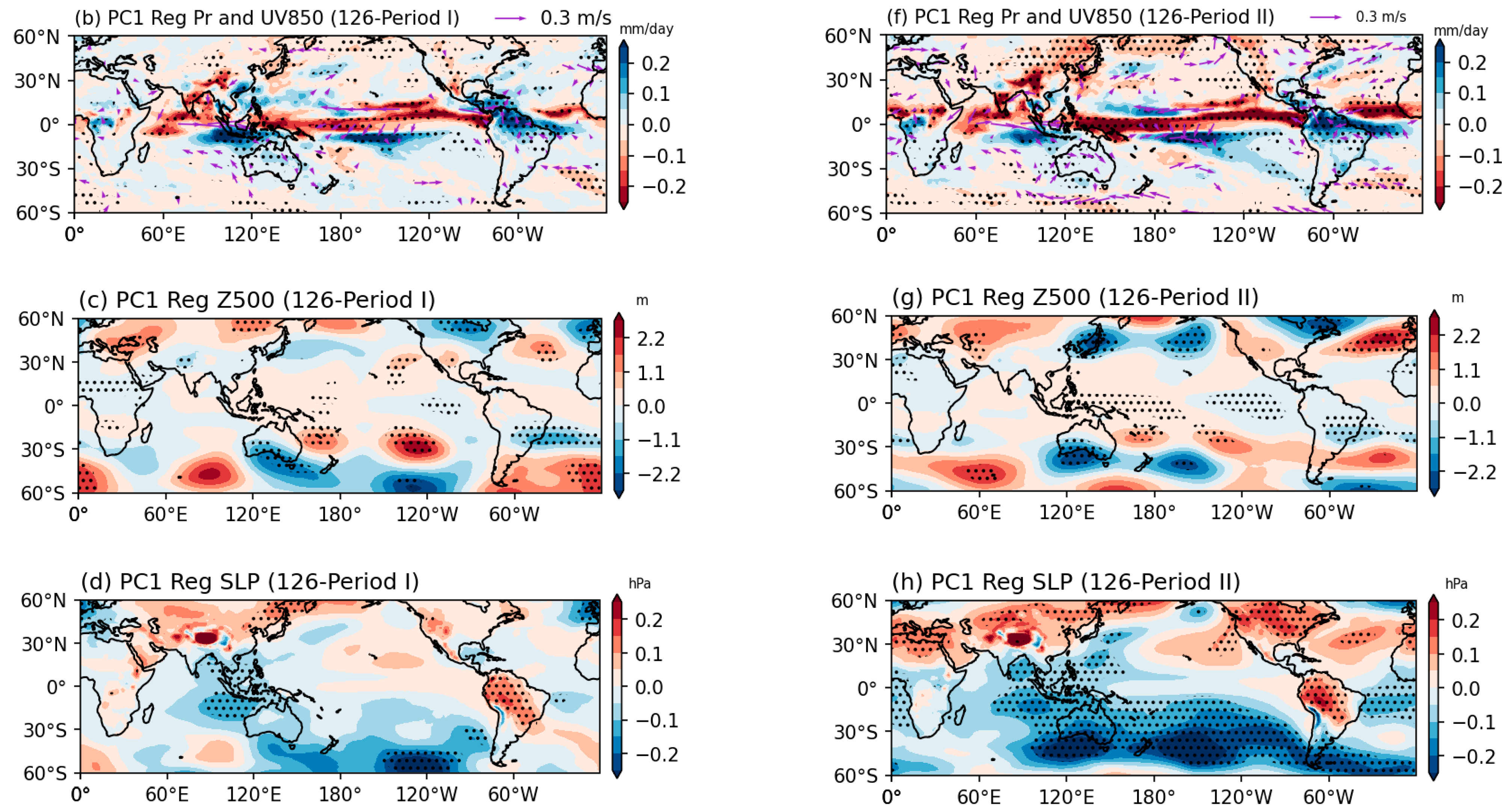
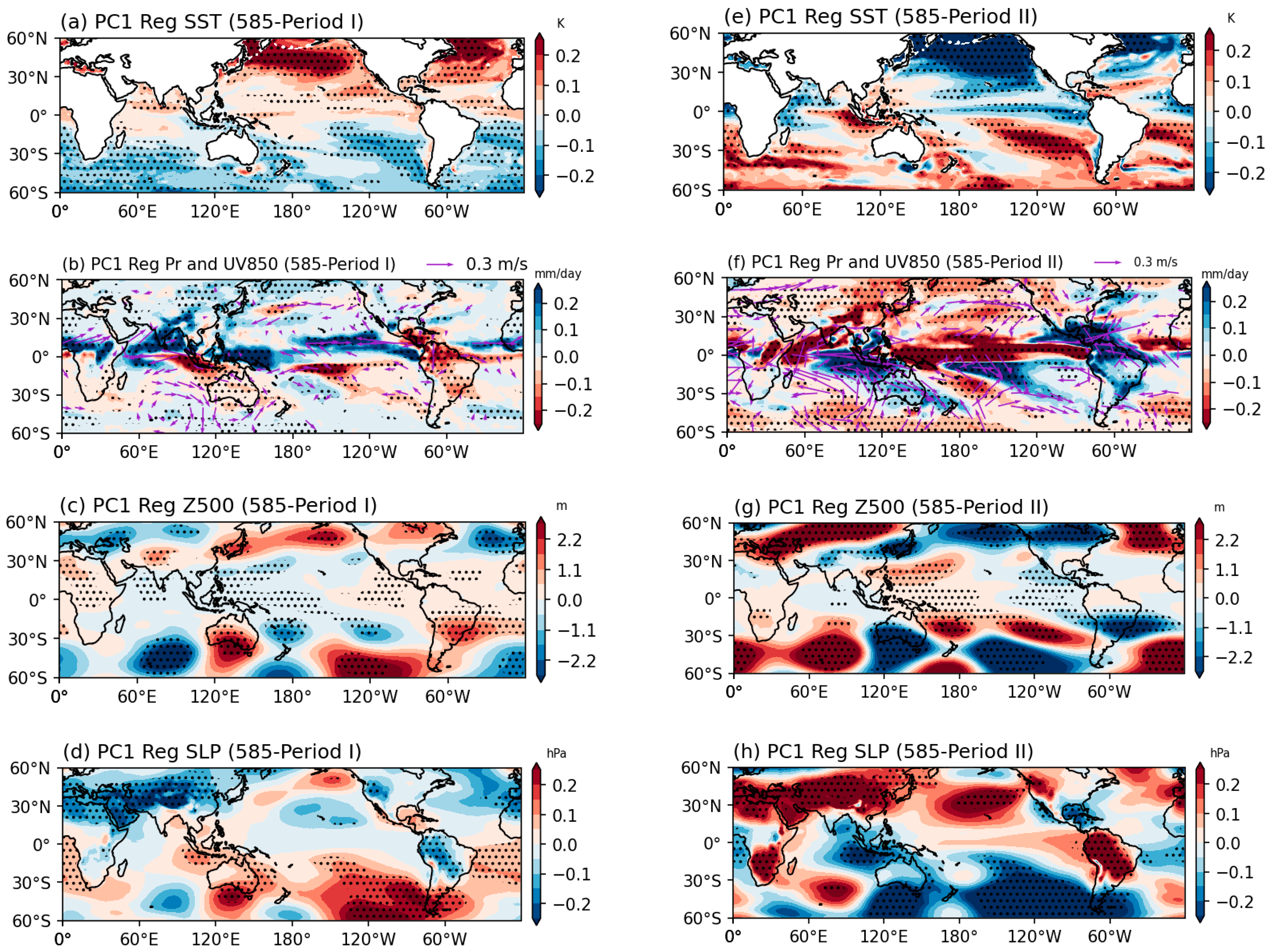
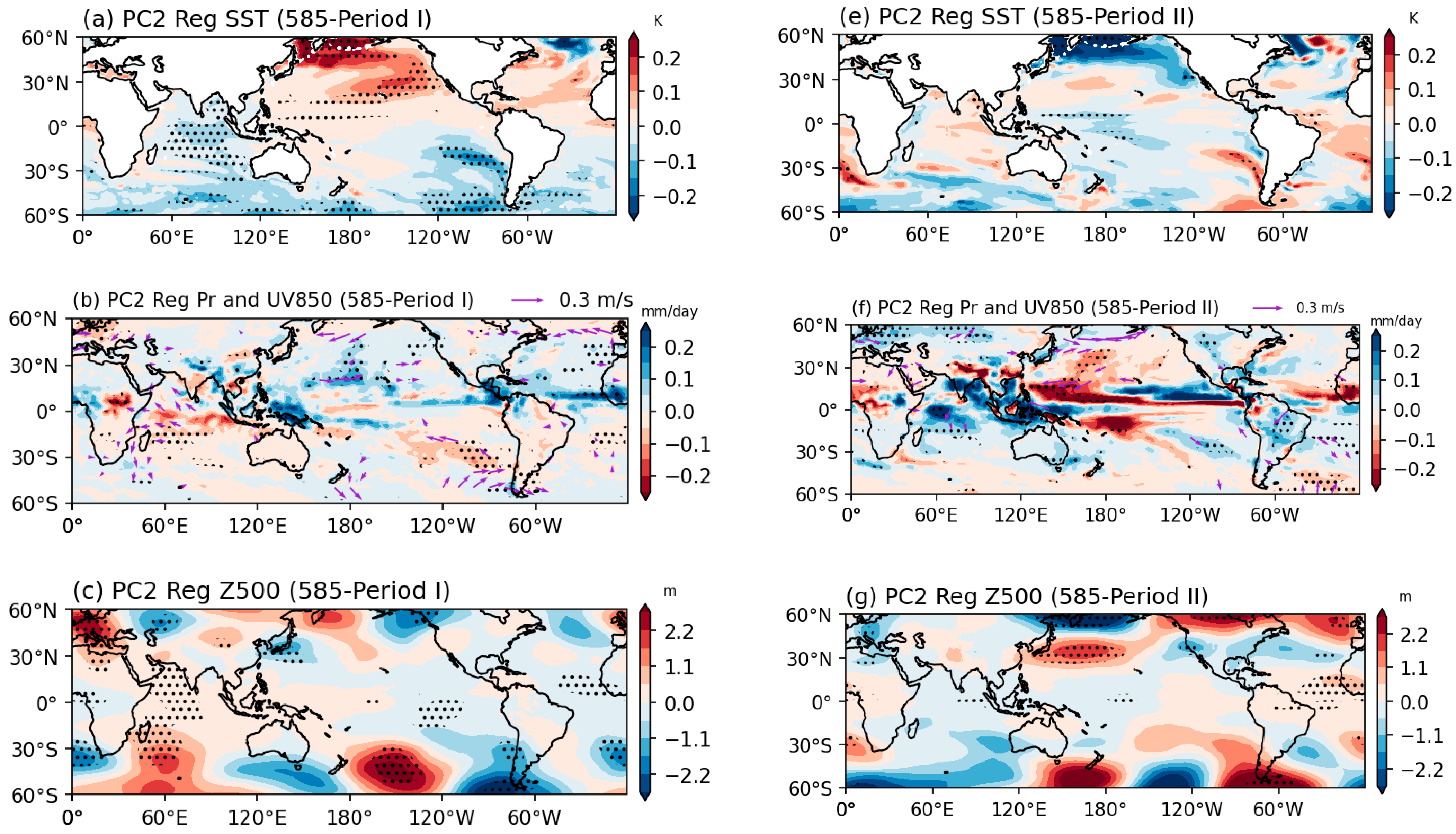
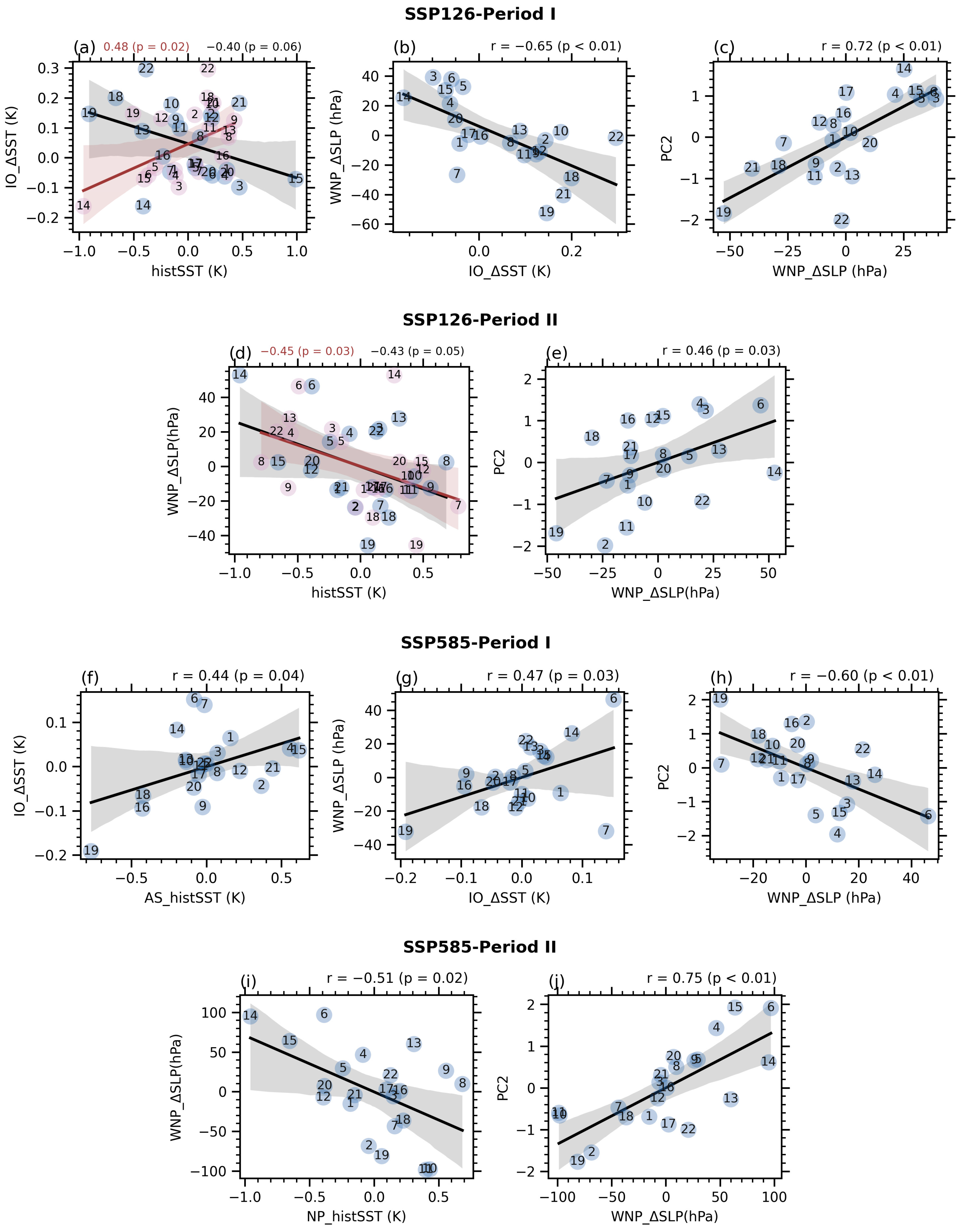
For SSP126 Period II and SSP585 Period I, which are mainly affected by South Atlantic SST anomalies, regression of PC1 onto atmospheric fields indicates that both periods influence East Asian climate primarily through Pacific-South American (PSA)-type Rossby wave trains, but with opposite phases (Figure 14e–h and Figure 15a–d).

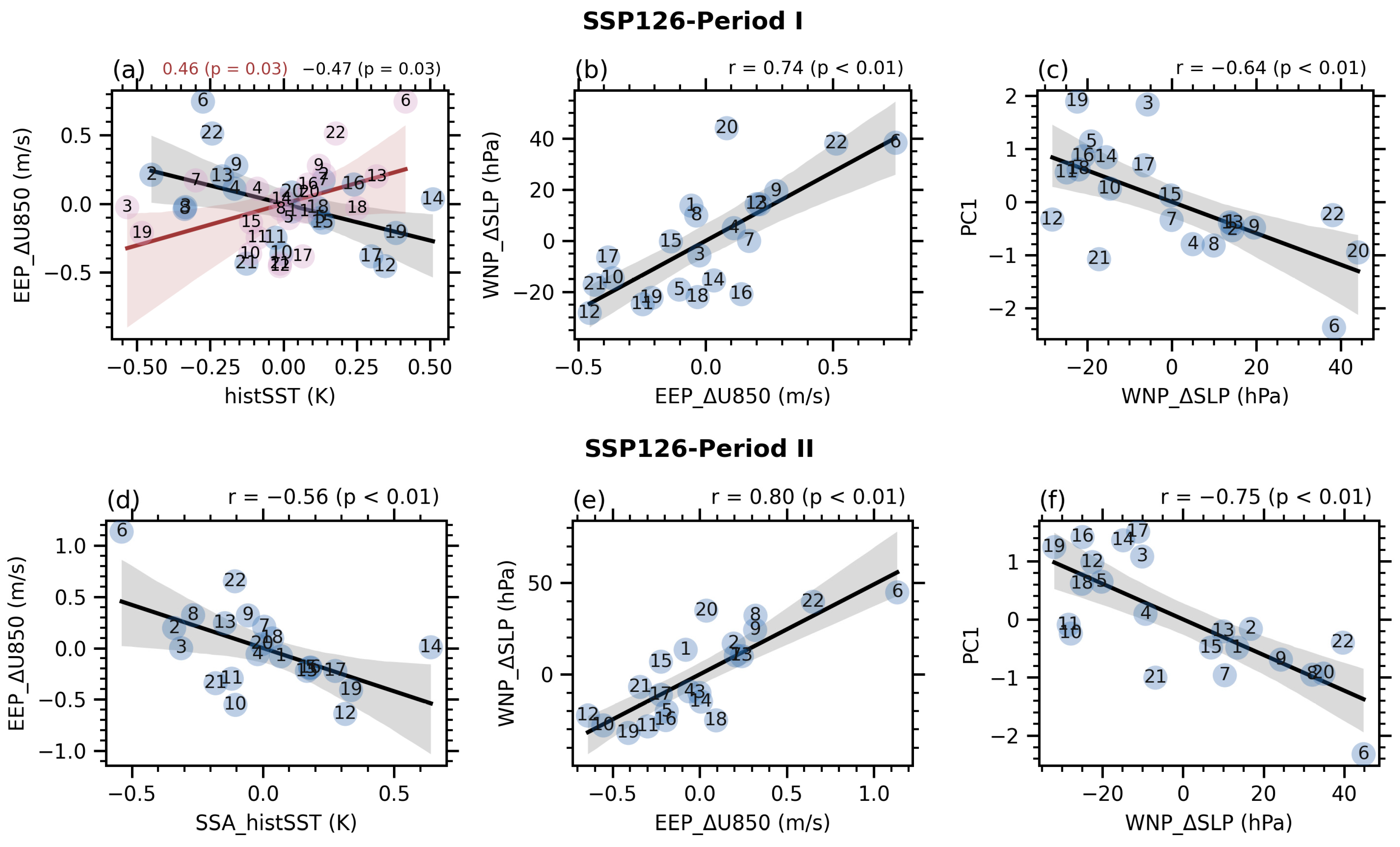
During SSP126 Period II, warmer historical SSTs in the South Atlantic can trigger a positive-phase PSA wave train [31], inducing an anomalous anticyclone over the subtropical southeastern Pacific. This enhances the cross-equatorial southeasterly trade winds as well as Ekman offshore transport and cold-water upwelling in the equatorial eastern Pacific, leading to the development of cold tongue-like SST anomalies [32] (Figure 14e). The wave train subsequently propagates westward, inducing an anomalous anticyclone in the mid-to-high latitudes of the southern Indian Ocean. Through anomalous westerlies over the central Indian Ocean and wind-evaporation-SST (WES) feedback, SSTs become cooler in the Arabian Sea and Bay of Bengal but warmer in the warm pool east of the Philippines, forming a negative-phase Indian Ocean Dipole (IOD)-like SST pattern [33]. Meanwhile, pronounced low-level cyclonic anomalies develop from the tropical Indian Ocean-maritime continent region to the western North Pacific (Figure 14f–h and Figure 16d–f). Under these conditions, Guangdong is located on the northwestern flank of the cyclonic circulation, where enhanced southerly or southeasterly winds strengthen moisture transport and low-level convergence, increasing precipitation and thereby weakening compound dry-hot events.

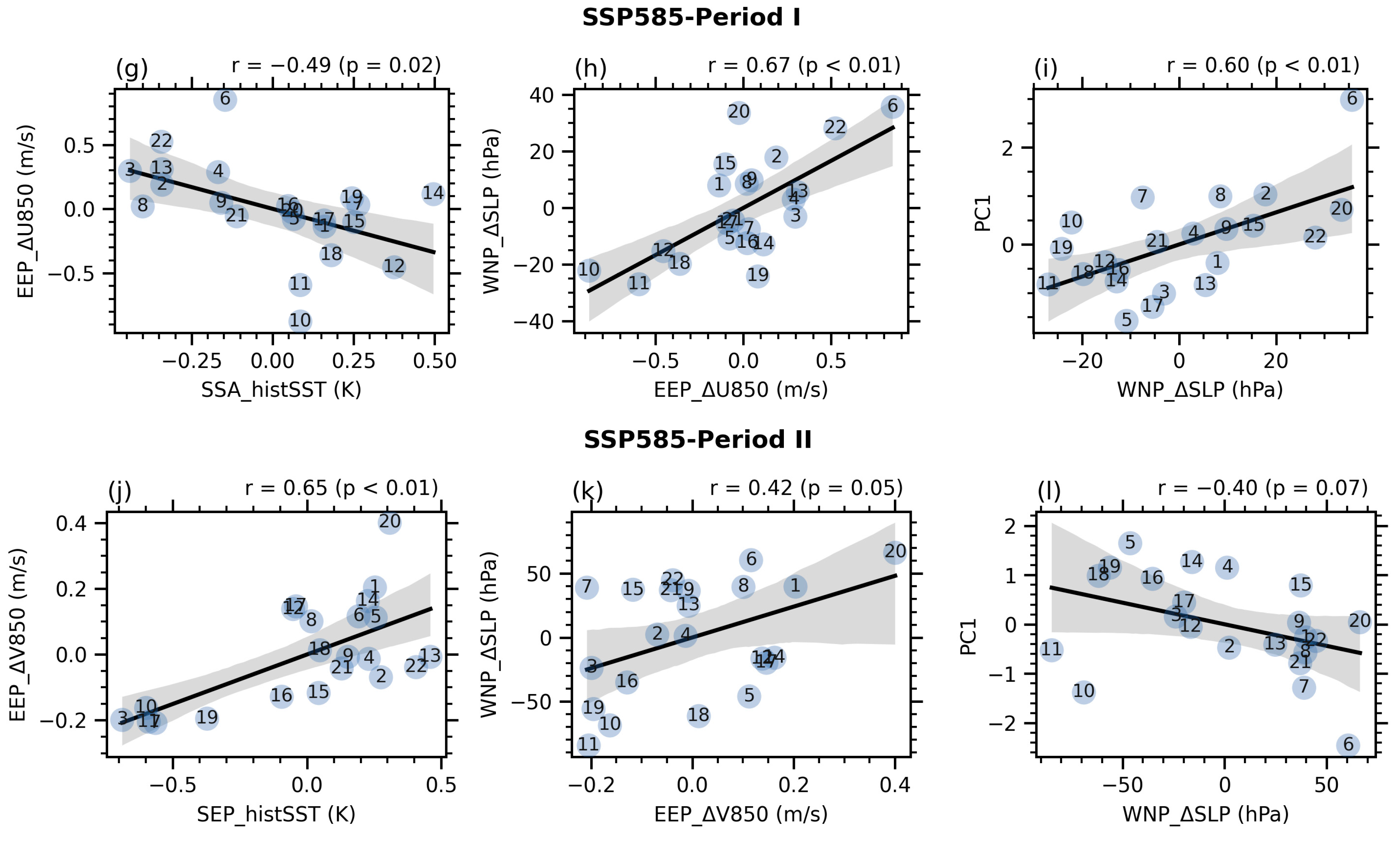
In contrast, during SSP585 Period I, colder historical SSTs in the key region trigger a negative-phase PSA wave train, inducing an anomalous cyclone over the subtropical southeastern Pacific. This suppresses the southeasterly trade winds and cold-water upwelling and, through the Bjerknes positive feedback, promotes the development of El Niño-like warm anomalies in the equatorial eastern Pacific (Figure 15a). The wave train then propagates westward, generating easterly wind anomalies over the central Indian Ocean that drive warm-water transport from the western Pacific warm pool eastward. As a result, SSTs become warmer in the Arabian Sea and Bay of Bengal but cooler east of the Philippines, forming a positive-phase IOD-like SST pattern and establishing an anomalous anticyclonic circulation over the South China Sea-Philippine region (Figure 15b–d and Figure 16g–i). Easterly anomalies on its southern flank suppress the northward progression of the South China Sea summer monsoon, reducing moisture transport to Guangdong and leading to a marked intensification of compound dry-hot events.

On this basis, SSP126 Period I and SSP585 Period II further reflect the enhancing effects of additional key regions on the first leading mode (Figure 14a–d and Figure 15e–h).

For SSP126 Period I, in addition to the South Atlantic, the first mode is also constrained by cold SST anomalies in the central-eastern Pacific. These cold anomalies suppress local deep convection and reduce latent heat release, shifting the tropical Pacific convective center westward toward the western Pacific warm pool and strengthening the Walker circulation. The enhanced low-level easterlies further promote westward accumulation of surface waters and intensify Ekman divergence and cold-water upwelling in the equatorial eastern Pacific, facilitating the development and persistence of La Niña-like SST conditions (Figure 14a). The central-eastern Pacific cooling acts synergistically with changes in the South Pacific subtropical circulation to enhance the propagation and maintenance of the PSA wave train, making the anomalous subtropical anticyclone over the southeastern Pacific stronger and more persistent. This further modulates low-level circulation over the Indian Ocean and the western North Pacific, inducing more pronounced low-level cyclonic anomalies across the tropical Indian Ocean to the western North Pacific region [34] (Figure 14b–d and Figure 16a–c). As a result, moisture transport to Guangdong is more strongly enhanced, precipitation increases more markedly, and compound dry-hot events are more substantially weakened, indicating that incorporating the central-eastern Pacific constraint produces a synergistic enhancement with the South Atlantic forcing.

For SSP585 Period II, in addition to the positive-phase PSA wave train triggered by warm SST anomalies in the South Atlantic, warm SST anomalies in the subtropical eastern Pacific provide an additional thermal forcing source. This strengthens the wave activity flux from the South Pacific to the mid-to-high latitudes of the Pacific, making the PSA wave train more coherent, of larger amplitude, and more stable in its propagation [35]. Consequently, the anomalous subtropical anticyclone over the southeastern Pacific is further intensified. Southerly to southeasterly wind anomalies on its eastern flank favor enhanced offshore Ekman transport and coastal upwelling along the Peru-Chile coast [36]. Through modulation of wind stress curl, Ekman pumping, and thermocline structure, these processes promote and maintain the development of cold tongue-like SST anomalies in the equatorial eastern Pacific (Figure 15e). Meanwhile, the strengthened wave train continues to extend westward, amplifying the tropical atmospheric response and reinforcing low-level moisture transport, convergence, and the northward-propagating stationary Rossby wave response. This results in a stronger anomalous anticyclone over the North Pacific and more pronounced low-level cyclonic anomalies and moisture convergence from the tropical Indian Ocean-maritime continent region to the western North Pacific (Figure 15f–h and Figure 16j–l). Under the combined influence of strengthened southerly-southeasterly winds on the southwestern flank of the North Pacific subtropical high and the northwestern flank of the low-level cyclone, precipitation over Guangdong increases more significantly than under South Atlantic warming alone, leading to a stronger weakening effect on compound dry-hot events.

Compared with the first leading mode, the constrained key regions of the second leading mode exhibit larger inter-period differences but remain highly consistent across scenarios within the same period. For Period I, the key regions under SSP126 are located in the waters surrounding Australia and the South Pacific, whereas those under SSP585 are mainly confined to the waters near Australia, indicating that this region is the core area governing inter-model uncertainty in the second leading mode during Period I. For Period II, the key regions under SSP126 are situated in the North Pacific and North Atlantic. In contrast, under SSP585, the weakened meridional SST gradient anomalies between the tropical and subtropical North Pacific and North Atlantic result in the retention of only the North Pacific as the key region, indicating that the North Pacific is the primary sensitive area controlling inter-model uncertainty in the second leading mode during Period II.

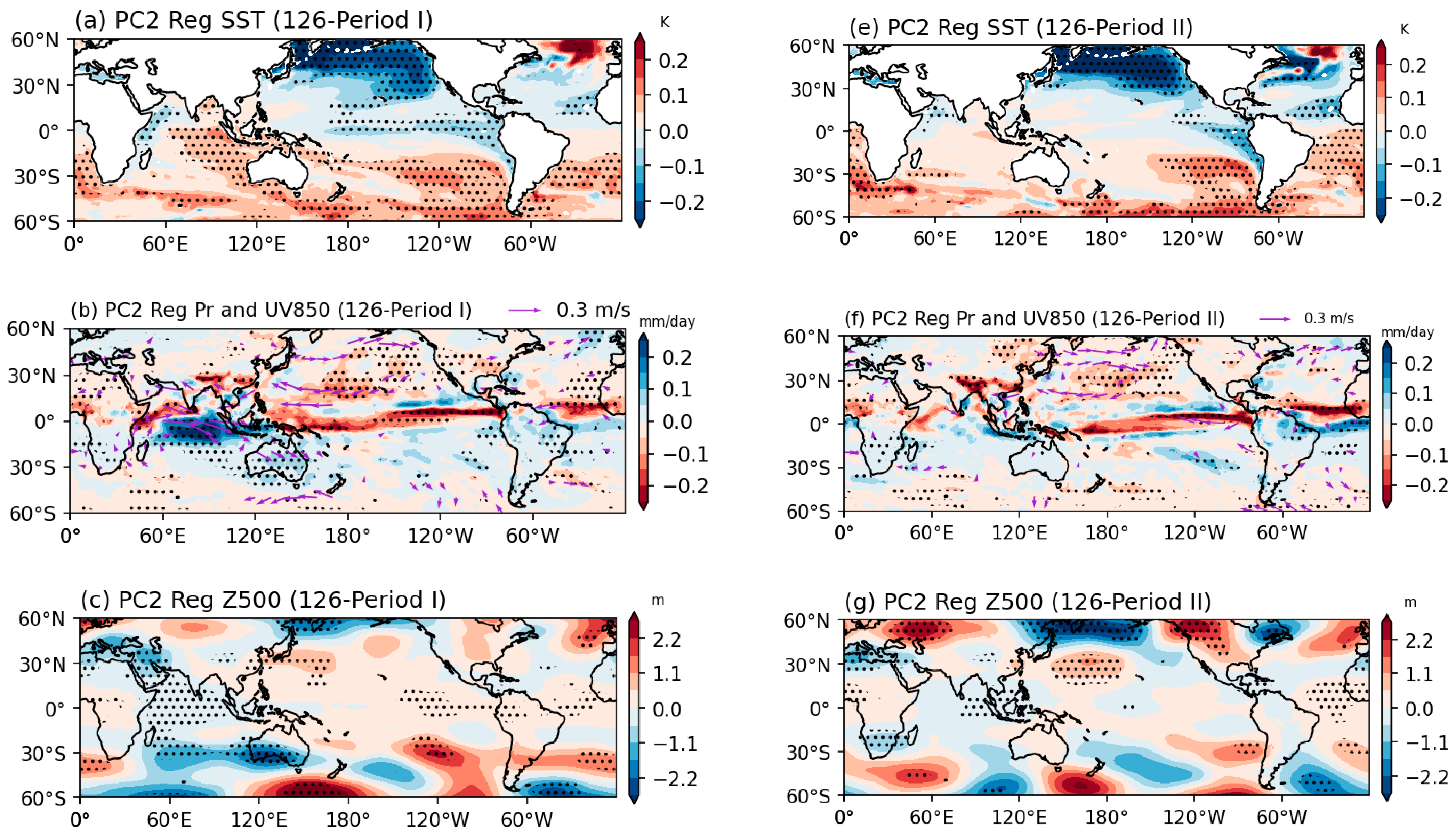
During Period I, the second leading mode primarily affects the spatial distribution of precipitation over Guangdong by modulating the Indian Ocean Basin Mode (IOBM) and its linkage with the western North Pacific circulation (Figure 17a–d and Figure 18a–d).

Under SSP126 Period I, warm SST anomalies near Australia enhance convection and latent heat release over the maritime continent and adjacent warm pool regions, inducing low-level cyclonic circulation anomalies and altering the background Walker circulation. Meanwhile, the eastern Indian Ocean experiences more pronounced warming due to heat transport by the Indonesian Throughflow and local anomalous heating. In contrast, cold SST anomalies over the South Pacific suppress local convection and strengthen the subtropical high and the equatorward southeasterly trade winds. The combined effects intensify equatorial easterly wind stress, promoting the development and persistence of La Niña-like SST conditions in the eastern Pacific (Figure 17a). Superimposed upon anomalous heating near Australia and regional air-sea coupling processes [37], the Indian Ocean exhibits basin-wide warming resembling a positive IOBM phase, accompanied by anomalous westerlies and negative sea-level pressure anomalies over the northern Indian Ocean. This warming modulates the western North Pacific and North Pacific circulation through adjustments of tropical circulation, leading to an anomalous anticyclone over the North Pacific (Figure 17b–d and Figure 19a–c). Consequently, moisture transport and convergence conditions over the South China Sea and South China are modified, resulting in increased precipitation over southern Guangdong and relatively reduced precipitation in the north, thereby producing a pronounced north-south precipitation contrast.

Under SSP585 Period I, cold SST anomalies near Australia suppress convection and induce anomalous high pressure. Enhanced offshore southeasterlies on its western flank strengthen coastal upwelling through evaporative cooling and Ekman offshore transport, markedly reducing SSTs from the northwestern coast of Australia to the southeastern Indian Ocean. Meanwhile, meridional Ekman transport driven by anomalous southeasterlies extends northward and westward, weakening the background westerlies over the equatorial Indian Ocean. Cold waters further propagate westward via advection, ultimately cooling the entire Indian Ocean basin and forming a negative IOBM phase [38] (Figure 18a). Following the suppression of Indian Ocean convection, convective activity shifts westward toward the western North Pacific warm pool and adjacent seas, inducing an anomalous low-level cyclonic circulation over the western North Pacific (Figure 18b–d and Figure 19f–h). Under these conditions, northern Guangdong lies near the convergence and ascending branch at the edge of the circulation, resulting in increased precipitation and relatively weakened dry-hot conditions. In contrast, southern Guangdong deviates from the main rain belt, leading to reduced precipitation and markedly intensified compound dry-hot events.

During Period II, the second leading mode is characterized by a pronounced strengthening of the western North Pacific subtropical anticyclone in both scenarios, although the formation mechanisms differ.

Under SSP126 Period II, the anomalous anticyclone is related not only to cold SST anomalies in the mid-to-high latitudes of the North Pacific but also to the combined modulation of a meridional SST gradient anomaly over the North Atlantic characterized by subtropical cooling and tropical warming. Cold SSTs in the North Pacific enhance lower-tropospheric stability and suppress sensible and latent heat fluxes, favoring the maintenance of low-level high-pressure anomalies and strengthening the North Pacific-western North Pacific anticyclonic circulation [39] (Figure 17e). This midlatitude high-pressure anomaly further excites and maintains stationary Rossby wave trains that propagate downstream toward Eurasia and the western North Pacific, thereby modulating low-level circulation over the Indo-Pacific region. Cyclonic anomalies and ascending motion are more likely to occur near the Bay of Bengal, while strengthened southwesterlies on its southern flank enhance warm and moist advection from the northern Indian Ocean, favoring sustained warming over the Bay of Bengal and northern Indian Ocean. Meanwhile, the intensified western North Pacific anticyclone maintains anomalous easterly or northeasterly winds on its southwestern flank, which converge with southwesterly warm and moist flows from the Bay of Bengal over the central South China Sea and coastal South China. Combined with warm SST anomalies in the South China Sea, this shifts the precipitation center toward coastal Guangdong, producing increased rainfall in the south and reduced rainfall in the north. Furthermore, meridional SST gradient anomalies in the North Atlantic amplify and reshape these coupled processes. Tropical North Atlantic warming adjusts the Indo-Pacific Walker circulation via atmospheric bridge processes, strengthening low pressure and ascending motion over the Indian Ocean-maritime continent region, enhancing the monsoon trough and moisture transport, and effectively weakening the western North Pacific anticyclone (Figure 19d, red contours). Subtropical North Atlantic cooling favors modulation of the midlatitude jet stream and waveguide conditions, facilitating downstream propagation of stationary wave trains toward Eurasia and the western North Pacific, where they constructively interfere with North Pacific high-pressure anomalies. The combined influence of these signals further strengthens equatorial easterly wind stress over the tropical Pacific, intensifying cold tongue-like SST anomalies in the central-eastern Pacific [40], thereby reinforcing the maintenance and constraint of the western North Pacific subtropical anticyclone (Figure 17f–h and Figure 19d–e).

Under SSP585 Period II, the physical mechanism is broadly similar to that under SSP126 Period II, with a marked strengthening of the western North Pacific subtropical anticyclone. The key difference is that SSP585 lacks the additional tropical heating and waveguide modulation associated with North Atlantic meridional SST gradient anomalies and is influenced mainly by North Pacific SST anomalies. Consequently, constraints on the tropical Pacific background state are relatively weaker, and the central-eastern Pacific cold tongue signal is weaker than under SSP126 (Figure 17e and Figure 18e). Nevertheless, the dominant circulation pattern and its control on the north-south precipitation contrast over Guangdong remain generally consistent with SSP126 Period II. Moreover, owing to the absence of North Atlantic SST anomalies, particularly the weakening effect of tropical North Atlantic warming on the western North Pacific anticyclone, the intensified western North Pacific subtropical anticyclone under SSP585 is even stronger than that under SSP126.

4.2. Implications for Climate Risk and Adaptation in Guangdong

The constrained SCEI projections indicate that the overall magnitude of future changes in Guangdong is smaller than that derived from the unconstrained multi-model ensemble mean. Moreover, in several scenarios and periods, spatial patterns characterized by widespread intensification in the unconstrained results shift to a coexistence of localized intensification and broad-scale weakening after constraint. This suggests that the unconstrained ensemble may overestimate the magnitude of future SCEI changes in Guangdong, whereas projections based on observational constraints provide more robust information on regional climate change. For climate risk assessment, directly adopting unconstrained results may exaggerate future risk levels and lead to overly conservative allocation of adaptation resources. In contrast, constrained projections provide a more reliable basis for decision-making that is better aligned with actual risk levels.

Spatially, the constrained changes exhibit pronounced regional heterogeneity. Western Guangdong and the southwestern coastal areas still show relatively large increases in SCEI under most scenarios and remain potential risk hotspots, particularly during the late period under SSP585. These regions therefore require priority in strengthening infrastructure resilience, improving monitoring and early-warning systems, and enhancing comprehensive disaster prevention capacity for extreme climate events. By contrast, northern and eastern Guangdong, as well as parts of the Pearl River Delta, show markedly reduced increases after constraint, with some areas even shifting to negative changes, indicating that future risk escalation in these regions is less severe than suggested by the unconstrained projections. Therefore, climate adaptation strategies in Guangdong should avoid a uniform policy framework and instead adopt region-specific and tiered adaptation measures based on the spatial heterogeneity revealed by the constrained projections.

Nevertheless, the constrained results do not imply negligible future risks. In particular, under the high-emission scenario during the late period, several regions in Guangdong still exhibit significant upward trends, indicating that regional climate risks may continue to accumulate under insufficient emission reductions. Therefore, the practical significance of this study does not lie in simply lowering risk estimates, but in enhancing the reliability of future regional risk assessments by reducing the influence of model biases, thereby providing a scientific basis for more targeted and phased climate adaptation policies in Guangdong.

5. Conclusions

This study aimed to correct biases in CMIP6 projections of compound dry-hot events (CDHEs) over Guangdong using an observational constraint approach, thereby improving the credibility of future risk assessments. For the dry-hot change indicator (ΔSCEI) in two future periods (Period I and Period II) under both the high-emission scenario (SSP585) and the low-emission scenario (SSP126), inter-model EOF decomposition was performed to extract the dominant modes of uncertainty. These modes were then regressed onto historical sea surface temperature (SST) fields to identify the key SST patterns that drive uncertainties. Based on the observational data, effective constraint relationships were constructed to calibrate future projections, and the underlying physical mechanisms were further investigated.

Both reanalysis data and CMIP6 simulations show that CDHEs in Guangdong intensify over time. The increase is much stronger under SSP585 than under SSP126, and stronger in Period II than in Period I, with more severe conditions in southern Guangdong than in the north. Meanwhile, CMIP6 models exhibit substantial differences in future SCEI projections. Overall, inter-model spread is larger under SSP585 than under SSP126, and larger in Period I than in Period II, with the smallest spread occurring in SSP585-Period II. Except for the relatively high uncertainty over western Guangdong under SSP585-Period II, model uncertainty is generally higher in northern Guangdong than in southern Guangdong.

EOF decomposition shows that the main source of projection uncertainty can be captured by the first two leading modes. Under SSP126, the first two modes explain more than 95% of the total variance in both periods; under SSP585, they explain nearly 95% in Period I and more than 95% in Period II. In both scenarios and periods, the first mode exhibits a monopole structure. It is a positive monopole only in SSP585-Period I and a negative monopole in all other cases. The second mode consistently shows a north-south dipole structure. It displays positive anomalies in the south and negative anomalies in the north only in SSP585-Period I, whereas all other periods exhibit the opposite pattern, with positive anomalies in the north and negative anomalies in the south.

After identifying the dominant modes of projection uncertainty, we further linked them to historically simulated SST fields to diagnose the key SST patterns driving the uncertainties and to establish present-future constraint relationships. The results show that, after applying the constraints, inter-model uncertainty is reduced by about 63% and 77% in Period I and Period II under SSP126, and by about 57% and 59% under SSP585, with the most robust constraint effect occurring in SSP126-Period II.

The historical SST patterns associated with each dominant mode can modulate future large-scale environmental fields through specific physical mechanisms and further influence multiscale circulation responses, thereby governing inter-model differences in projected SCEI changes. This causal linkage reduces uncertainty in future SCEI projections at the source. The constrained projections show that, under the high-emission scenario SSP585, Guangdong will face a marked increase in CDHE risk in Period II. This is mainly associated with historical warm biases in the eastern Pacific and South Atlantic and cold biases in the North Pacific. After correcting these SST biases, the effects associated with the strengthening of the PSA-type wave train and the western North Pacific subtropical anticyclone are suppressed, producing a north-to-south increasing gradient of dry-hot intensification across Guangdong, with the strongest signal in western Guangdong.

By contrast, constrained CDHE changes in the other periods generally weaken to varying degrees, although western Guangdong still shows different levels of intensification in all periods. Specifically, in SSP585-Period I, correcting the cold biases in the South Atlantic and waters near Australia suppresses the future impacts associated with the PSA-type wave train and basin-wide cold SST anomalies in the Indian Ocean, leading to a marked weakening of dry-hot conditions across the province, although slight intensification persists over the Leizhou Peninsula. In SSP126-Period I, correcting the warm biases in the South Atlantic and waters near Australia suppresses the future impacts associated with the strengthened PSA-type wave train and basin-wide warm SST anomalies in the Indian Ocean, producing a north-to-south transition from weakening to intensification across Guangdong, with more severe future CDHEs in southern Guangdong. In SSP126-Period II, correcting the cold biases in the South Atlantic, North Pacific, and North Atlantic suppresses the future impacts associated with the strengthened PSA-type wave train and the marked enhancement of the western North Pacific subtropical anticyclone, resulting in a spatial pattern of CDHEs broadly similar to that in SSP126-Period I, although the severity is slightly weaker over the south-central region.

This study demonstrates a stable link between historical SST modes and inter-model differences in future projections, providing a new pathway for reducing projection uncertainty using observational information and offering important scientific support for regional-scale climate risk assessment and adaptation planning. Although the observational constraint method substantially reduces uncertainties in CMIP6 projections of future CDHEs over Guangdong, its effectiveness remains dependent on the quality of historical observations and the ability of the models to represent key SST-atmosphere interaction processes. Because reanalysis datasets are influenced by data assimilation systems and model assumptions, the constrained results essentially represent an “optimal estimate under reanalysis constraints,” and related uncertainties are not fully eliminated. Future studies should further assess the robustness and transferability of constraint relationships by integrating high-quality station observations, additional multisource datasets, and regional climate model simulations.

References

1. Calvin, K.; Dasgupta, D.; Krinner, G.; Mukherji, A.; Thorne, P.W.; Trisos, C.; Romero, J.; Aldunce, P.; Barrett, K.; Blanco, G.; et al. IPCC, 2023: Climate Change 2023: Synthesis Report, 1st ed.; Contribution of Working Groups I, II and III to the Sixth Assessment Report of the Intergovernmental Panel on Climate Change; Core Writing Team, Lee, H., Romero, J., Eds.; Intergovernmental Panel on Climate Change (IPCC): Geneva, Switzerland, 2023. [Google Scholar]
2. Hao, Z. Compound Events and Associated Impacts in China. iScience 2022, 25, 104689. [Google Scholar] [CrossRef] [Scilit]
3. AghaKouchak, A.; Cheng, L.; Mazdiyasni, O.; Farahmand, A. Global Warming and Changes in Risk of Concurrent Climate Extremes: Insights from the 2014 California Drought. Geophys. Res. Lett. 2014, 41, 8847–8852. [Google Scholar] [CrossRef] [Scilit]
4. Miralles, D.G.; Gentine, P.; Seneviratne, S.I.; Teuling, A.J. Land-Atmospheric Feedbacks during Droughts and Heatwaves: State of the Science and Current Challenges. Ann. N. Y. Acad. Sci. 2019, 1436, 19–35. [Google Scholar] [CrossRef] [Scilit]
5. Ye, L.; Shi, K.; Xin, Z.; Wang, C.; Zhang, C. Compound Droughts and Heat Waves in China. Sustainability 2019, 11, 3270. [Google Scholar] [CrossRef] [Scilit]
6. Otto, F.E.L.; Massey, N.; Van Oldenborgh, G.J.; Jones, R.G.; Allen, M.R. Reconciling Two Approaches to Attribution of the 2010 Russian Heat Wave. Geophys. Res. Lett. 2012, 39, 2011GL050422. [Google Scholar] [CrossRef] [Scilit]
7. Zheng, J.; Liu, W.; Li, W.; Zhuang, Y. Climatological Characteristics for Guangdong Province in 2022 and the Effect Discussion. Guangdong Meteorol. 2024, 46, 9–13. [Google Scholar] [CrossRef]
8. Eyring, V.; Bony, S.; Meehl, G.A.; Senior, C.A.; Stevens, B.; Stouffer, R.J.; Taylor, K.E. Overview of the Coupled Model Intercomparison Project Phase 6 (CMIP6) Experimental Design and Organization. Geosci. Model Dev. 2016, 9, 1937–1958. [Google Scholar] [CrossRef] [Scilit]
9. Zhou, T.; Chen, Z.; Zou, L.; Chen, X.; Yu, Y.; Wang, B.; Bao, Q.; Bao, Y.; Cao, J.; He, B.; et al. Development of Climate and Earth System Models in China: Past Achievements and New CMIP6 Results. J. Meteorol. Res. 2020, 34, 1–19. [Google Scholar] [CrossRef] [Scilit]
10. Petrova, I.Y.; Miralles, D.G.; Brient, F.; Donat, M.G.; Min, S.-K.; Kim, Y.-H.; Bador, M. Observation-Constrained Projections Reveal Longer-than-Expected Dry Spells. Nature 2024, 633, 594–600. [Google Scholar] [CrossRef] [Scilit]
11. Yao, L.; Leng, G.; Yu, L.; Tu, H.; Qiu, J. Observational Constraint on Climate Model Projections of Global Compound Hot-Dry Events and the Socioeconomic Risks under Climate Change. Environ. Res. Lett. 2024, 19, 114027. [Google Scholar] [CrossRef] [Scilit]
12. Bole, Y.; Guga, S.; Riao, D.; Zhang, J.; Tong, Z.; Liu, X. Emergency Constraint-Based CMIP6 Predictions for Future Droughts on the Mongolian Plateau. J. Hydrol. 2024, 645, 132156. [Google Scholar] [CrossRef] [Scilit]
13. Chen, Z.; Zhou, T.; Chen, X.; Zhang, W.; Zuo, M.; Man, W.; Qian, Y. Emergent Constrained Projections of Mean and Extreme Warming in China. Geophys. Res. Lett. 2023, 50, e2022GL102124. [Google Scholar] [CrossRef] [Scilit]
14. Bevacqua, E.; Zappa, G.; Lehner, F.; Zscheischler, J. Precipitation Trends Determine Future Occurrences of Compound Hot-Dry Events. Nat. Clim. Change 2022, 12, 350–355. [Google Scholar] [CrossRef] [Scilit]
15. Hosseinzadehtalaei, P.; Termonia, P.; Tabari, H. Projected Changes in Compound Hot-Dry Events Depend on the Dry Indicator Considered. Commun. Earth Environ. 2024, 5, 220. [Google Scholar] [CrossRef] [Scilit]
16. Brient, F. Reducing Uncertainties in Climate Projections with Emergent Constraints: Concepts, Examples and Prospects. Adv. Atmos. Sci. 2020, 37, 1–15. [Google Scholar] [CrossRef] [Scilit]
17. Hall, A.; Cox, P.; Huntingford, C.; Klein, S. Progressing Emergent Constraints on Future Climate Change. Nat. Clim. Change 2019, 9, 269–278. [Google Scholar] [CrossRef] [Scilit]
18. Maraun, D.; Shepherd, T.G.; Widmann, M.; Zappa, G.; Walton, D.; Gutiérrez, J.M.; Hagemann, S.; Richter, I.; Soares, P.M.M.; Hall, A.; et al. Towards Process-Informed Bias Correction of Climate Change Simulations. Nat. Clim. Change 2017, 7, 764–773. [Google Scholar] [CrossRef] [Scilit]
19. Freychet, N.; Hegerl, G.; Mitchell, D.; Collins, M. Future Changes in the Frequency of Temperature Extremes May Be Underestimated in Tropical and Subtropical Regions. Commun. Earth Environ. 2021, 2, 28. [Google Scholar] [CrossRef] [Scilit]
20. Zhu, H.; Jiang, Z.; Li, L.; Li, W.; Jiang, S. Improve the Projection of East China Summer Precipitation with Emergent Constraints. npj Clim. Atmos. Sci. 2024, 7, 298. [Google Scholar] [CrossRef] [Scilit]
21. Copernicus Climate Change Service. ERA5 Monthly Averaged Data on Pressure Levels from 1940 to Present. 2019. Available online: https://cds.climate.copernicus.eu/datasets/reanalysis-era5-pressure-levels-monthly-means?tab=overview (accessed on 12 January 2026).
22. Huang, B.; Thorne, P.W.; Banzon, V.F.; Boyer, T.; Chepurin, G.; Lawrimore, J.H.; Menne, M.J.; Smith, T.M.; Vose, R.S.; Zhang, H.-M. NOAA Extended Reconstructed Sea Surface Temperature (ERSST), Version 5, 2017. NOAA National Centers for Environmental Information. Available online: https://psl.noaa.gov/data/gridded/data.noaa.ersst.v5.html (accessed on 12 January 2026). [CrossRef]
23. Zscheischler, J.; Michalak, A.M.; Schwalm, C.; Mahecha, M.D.; Huntzinger, D.N.; Reichstein, M.; Berthier, G.; Ciais, P.; Cook, R.B.; El-Masri, B.; et al. Impact of Large-scale Climate Extremes on Biospheric Carbon Fluxes: An Intercomparison Based on MsTMIP Data. Glob. Biogeochem. Cycles 2014, 28, 585–600. [Google Scholar] [CrossRef] [Scilit]
24. McKee, T.B.; Doesken, N.J.; Kleist, J. The Relationship of Drought Frequency and Duration to Time Scales. In Proceedings of the 8th Conference on Applied Climatology, Anaheim, CA, USA, 17–22 January 1993; pp. 179–184. [Google Scholar]
25. Hao, Z.; Hao, F.; Singh, V.P.; Zhang, X. Statistical Prediction of the Severity of Compound Dry-Hot Events Based on El Niño-Southern Oscillation. J. Hydrol. 2019, 572, 243–250. [Google Scholar] [CrossRef] [Scilit]
26. Gringorten, I.I. A Plotting Rule for Extreme Probability Paper. J. Geophys. Res. 1963, 68, 813–814. [Google Scholar] [CrossRef] [Scilit]
27. Nelsen, R.B. An Introduction to Copulas, 2nd ed.; Springer Series in Statistics; Springer: New York, NY, USA, 2006. [Google Scholar]
28. Akaike, H. A New Look at the Statistical Model Identification. IEEE Trans. Automat. Contr. 1974, 19, 716–723. [Google Scholar] [CrossRef] [Scilit]
29. Tang, T.; Qi, L.; Tozuka, T.; Luo, J.-J.; Ling, F.; Luo, L.; He, J.-H. Emergent Constraint on the Projected Central Equatorial Pacific Warming and Northwestern Pacific Monsoon Trough Change. Environ. Res. Lett. 2024, 19, 054003. [Google Scholar] [CrossRef] [Scilit]
30. Chen, X.; Zhou, T.; Wu, P.; Guo, Z.; Wang, M. Emergent Constraints on Future Projections of the Western North Pacific Subtropical High. Nat. Commun. 2020, 11, 2802. [Google Scholar] [CrossRef] [Scilit]
31. Okumura, Y.M. Origins of Tropical Pacific Decadal Variability: Role of Stochastic Atmospheric Forcing from the South Pacific. J. Clim. 2013, 26, 9791–9796. [Google Scholar] [CrossRef] [Scilit]
32. Heede, U.K.; Fedorov, A.V. Colder Eastern Equatorial Pacific and Stronger Walker Circulation in the Early 21st Century: Separating the Forced Response to Global Warming From Natural Variability. Geophys. Res. Lett. 2023, 50, e2022GL101020. [Google Scholar] [CrossRef] [Scilit]
33. Sun, Y.; Zhu, Z.; Yang, Y.; Lu, R. Decadal Change in the Connection between the Pacific-Japan Pattern and the Indian Ocean SST Basin Mode. Clim. Dyn. 2024, 62, 4281–4296. [Google Scholar] [CrossRef] [Scilit]
34. Chen, Z.; Wen, Z.; Wu, R.; Du, Y. Roles of Tropical SST Anomalies in Modulating the Western North Pacific Anomalous Cyclone during Strong La Niña Decaying Years. Clim. Dyn. 2017, 49, 633–647. [Google Scholar] [CrossRef] [Scilit]
35. Freitas, A.C.V.; Rao, V.B.; Braga, H.A.; Ambrizzi, T. Rossby Wave Propagation in the Transition Seasons. Clim. Dyn. 2024, 62, 6893–6912. [Google Scholar] [CrossRef] [Scilit]
36. Bravo, L.; Ramos, M.; Astudillo, O.; Dewitte, B.; Goubanova, K. Seasonal Variability of the Ekman Transport and Pumping in the Upwellingsystem off Central-Northern Chile (∼30° S) Based on Ahigh-Resolution Atmospheric Regional Model (WRF). Ocean Sci. 2016, 12, 1049–1065. [Google Scholar] [CrossRef] [Scilit]
37. Feng, M.; McPhaden, M.J.; Xie, S.-P.; Hafner, J. La Niña Forces Unprecedented Leeuwin Current Warming in 2011. Sci. Rep. 2013, 3, 1277. [Google Scholar] [CrossRef] [Scilit]
38. Chen, M.; Collins, M.; Yu, J.-Y.; Wang, X.; Zhang, L.; Tam, C.-Y. Emerging Influence of the Australian Monsoon on Indian Ocean Interannual Variability in a Warming Climate. npj Clim. Atmos. Sci. 2024, 7, 319. [Google Scholar] [CrossRef] [Scilit]
39. Peng, D.; Zhou, T.; Hu, S.; Zheng, J. Ocean-Driven Shifts in Circulation Regime Frequency Modulate South China Rainfall. npj Clim. Atmos. Sci. 2025, 8, 379. [Google Scholar] [CrossRef] [Scilit]
40. An, X.; Chen, W.; Shi, J.; Luo, Y. Subtropical Jet Wave Train Associated with North Atlantic SST Contributes to ENSO-Like Anomalies. Geophys. Res. Lett. 2025, 52, e2025GL116621. [Google Scholar] [CrossRef] [Scilit]
Figure 1. Study area: (a) China and (b) Guangdong Province.
Atmosphere 17 00327 g001
Figure 2. Temporal evolution of temperature, precipitation, and SCEI projections, as well as associated uncertainties, under the SSP1-2.6 and SSP5-8.5 scenarios toward the end of the 21st century. (ac) The shaded areas indicate the range of simulations from multiple climate models. The green and purple solid lines represents the multi-model ensemble means (MME) under SSP1-2.6 and SSP5-8.5, respectively, while the red solid line shows the ERA5 reanalysis dataset. Green and purple error bars correspond to the SSP1-2.6 and SSP5-8.5 scenarios, respectively. Colors from light to dark indicate Period I and Period II. The error bars show the maximum, minimum, and interquartile ranges, and the green and purple text above indicates the coefficients of variation (CV; standard deviation normalized by the mean), with color meanings consistent with those of the error bars.
Atmosphere 17 00327 g002
Figure 3. SSP126 and SSP585 Spatial distribution of the relative change in SCEI (relative to 1961–2014) and its uncertainty ( σ ) based on the multi-model ensemble (MME).
Atmosphere 17 00327 g003aAtmosphere 17 00327 g003b
Figure 4. SSP585 leading modes of projected uncertainty. (I,II) represent Period I and Period II, respectively. (a,b,e,f) show EOF1 and EOF2, the two leading modes derived from inter-model EOF analysis of projected SCEI changes. The values in the upper-right corners indicate the fraction of inter-model variance explained. Panels (c,d,g,h) show the corresponding normalized principal components (PC1 and PC2). Each number on the x-axis represents one of the 22 models.
Atmosphere 17 00327 g004aAtmosphere 17 00327 g004b
Figure 5. SSP126 leading modes of projected uncertainty. (I,II) represent Period I and Period II, respectively. (a,b,e,f) show EOF1 and EOF2, the two leading modes derived from inter-model EOF analysis of projected SCEI changes. The values in the upper-right corners indicate the fraction of inter-model variance explained. Panels (c,d,g,h) show the corresponding normalized principal components (PC1 and PC2). Each number on the x-axis represents one of the 22 models.
Atmosphere 17 00327 g005
Figure 6. SSP585 Historical SST patterns associated with the principal components (PCs). (I,II) represent Period I and Period II, respectively. The purple solid boxes indicate the regions used to define constraint indices for each PC. To minimize the influence of global-scale SST simulation biases, the tropical mean SST (30° S-30° N) was removed from each model before regression. Hatched shading indicates regions where the regression is statistically significant at the 5% level based on a Student’s t-test.
Atmosphere 17 00327 g006
Figure 7. As Figure 6, but for the SSP126.
Atmosphere 17 00327 g007
Figure 8. (a,b) Inter-model emergent relationships under SSP585 Period I, showing the relationships between projections (PCs) and historical temperature pattern (IDs). The black solid line represents the linear regression line, and the gray shaded area indicates the 95% confidence interval of the regression. The blue and purple vertical dashed lines represent SST observed values. The red vertical dashed line denotes the mean value of the observational dataset, while the red horizontal dashed line indicates the optimal projection induced by the emergent constraint. Each gray number denotes one of the 22 models. (c,d) Probability density function of original and constrained future projections. The values in parentheses indicate the mean and standard deviation of the Gaussian distribution. Black circles denote the original PC values of each model.
Atmosphere 17 00327 g008
Figure 9. (a,b) Inter-model emergent relationships under SSP585 Period II, showing the relationships between projections (PCs) and historical temperature pattern (IDs). The black solid line represents the linear regression line, and the gray shaded area indicates the 95% confidence interval of the regression. The blue and purple vertical dashed lines represent SST observed values. The red vertical dashed line denotes the mean value of the observational dataset, while the red horizontal dashed line indicates the optimal projection induced by the emergent constraint. Each gray number denotes one of the 22 models. (c,d) Probability density function of original and constrained future projections. The values in parentheses indicate the mean and standard deviation of the Gaussian distribution. Black circles denote the original PC values of each model.
Atmosphere 17 00327 g009
Figure 10. (a,b) Inter-model emergent relationships under SSP126 Period I, showing the relationships between projections (PCs) and historical temperature pattern (IDs). The black solid line represents the linear regression line, and the gray shaded area indicates the 95% confidence interval of the regression. The blue and purple vertical dashed lines represent SST observed values. The red vertical dashed line denotes the mean value of the observational dataset, while the red horizontal dashed line indicates the optimal projection induced by the emergent constraint. Each gray number denotes one of the 22 models. (c,d) Probability density function of original and constrained future projections. The values in parentheses indicate the mean and standard deviation of the Gaussian distribution. Black circles denote the original PC values of each model.
Atmosphere 17 00327 g010
Figure 11. (a,b) Inter-model emergent relationships under SSP126 Period II, showing the relationships between projections (PCs) and historical temperature pattern (IDs). The black solid line represents the linear regression line, and the gray shaded area indicates the 95% confidence interval of the regression. The blue and purple vertical dashed lines represent SST observed values. The red vertical dashed line denotes the mean value of the observational dataset, while the red horizontal dashed line indicates the optimal projection induced by the emergent constraint. Each gray number denotes one of the 22 models. (c,d) Probability density function of original and constrained future projections. The values in parentheses indicate the mean and standard deviation of the Gaussian distribution. Black circles denote the original PC values of each model.
Atmosphere 17 00327 g011
Figure 12. Constrained projection and its difference from the unconstrained results. (a,d,g,j) Unconstrained (UnCor) and (b,e,h,k) constrained (Cor) MME projections of SCEI based on the optimal estimated principal components. (c,f,i,l) Difference between the constrained and unconstrained results, reconstructed from the two constrained leading modes of uncertainty.
Atmosphere 17 00327 g012
Figure 13. Dominant modes of the constrained inter-model spread are shown in panels (ah). Panels (ad) and (eh) correspond to the two periods under the SSP585 and SSP126 scenarios, respectively. These panels represent the two constrained leading EOF modes of inter-model SCEI changes derived from the optimal first and second principal components (PC1 and PC2).
Atmosphere 17 00327 g013
Figure 14. Physical mechanisms associated with projections and model uncertainty under SSP126 for Period I and Period II. Panels (ad) show the projected changes in SST, precipitation, 850-hPa wind fields, 500-hPa geopotential height, and sea level pressure (SLP) for Period I, while panels (eh) show the corresponding changes for Period II. All variables are regressed onto the first principal component (PC1). Dotted areas and 850-hPa wind vectors indicate statistical significance at the 10% level based on Student’s t-test.
Atmosphere 17 00327 g014aAtmosphere 17 00327 g014b
Figure 15. As Figure 14, but for the SSP585 (Period I and Period II) and its first principal component (PC1).
Atmosphere 17 00327 g015
Figure 16. Inter-model physical relationships between historical and projected spreads for the first leading mode under SSP126 and SSP585 during Period I and Period II. (ac) Inter-model relationships among historical SST biases over the subtropical South Atlantic (SSA, black solid lines), historical SST biases over the Central Pacific (CP, red solid lines), 850-hPa zonal winds (U850) over the eastern equatorial Pacific (EEP), sea level pressure (SLP) changes over the western North Pacific (WNP), and the first principal component (PC1) during Period I of SSP126. (df) Inter-model relationships among historical SST biases over the SSA, U850 over the EEP, SLP changes over the WNP, and the PC1 during Period II of SSP126. (gi) Same as Period II of SSP126, but for Period I of SSP585. (jl) Inter-model relationships among historical SST biases over the southeastern Pacific (SEP), 850-hPa meridional winds (V850) over the EEP, SLP changes over the WNP, and the PC1 during Period II of SSP585. Shaded areas indicate the 95% confidence intervals of the linear regressions. Values in the upper-right corner of each panel denote the correlation coefficients (r) and significance levels (p). Each number represents an individual model listed in Table 1. Based on Student’s t-test, all regression results are statistically significant at the 10% level. Regional definitions vary slightly among periods and scenarios. For Period I of SSP126, the SSA region is defined as 25° S-15° N, 60° W-0°, the CP region as 20° S-10° N, 110–170° W, the EEP region as 5° S-5° N, 80–110° W, and the WNP region as 0–25° N, 90–150° E. For Period II of SSP126, the SSA region is defined as 30° S-15° N, 40° W-0°, while the EEP and WNP regions are the same as those in Period I of SSP126. For Period I of SSP585, the SSA region is defined as 15° S-10° N, 60° W-0°, while the EEP and WNP regions are the same as those in Period I of SSP126. For Period II of SSP585, the SEP region is defined as 30° S-0°, 100–160° W, the EEP region as 10° S-0°, 100–150° W, and the WNP region as 0–25° N, 90–120° E.
Atmosphere 17 00327 g016aAtmosphere 17 00327 g016b
Figure 17. As Figure 14, but for the SSP126 (Period I and Period II) and its second principal component (PC2).
Atmosphere 17 00327 g017aAtmosphere 17 00327 g017b
Figure 18. As Figure 14, but for the SSP585 (Period I and Period II) and its second principal component (PC2).
Atmosphere 17 00327 g018aAtmosphere 17 00327 g018b
Figure 19. Inter-model physical relationships between historical and projected spreads for the second leading mode under SSP126 and SSP585 during Period I and Period II. (ac) Inter-model relationships among historical SST biases over the Australian adjacent seas (AS, black solid lines), historical SST biases over the southern central Pacific (SCP, red solid lines), SST changes over the Indian Ocean (IO), SLP changes over the WNP, and the second principal component (PC2) during Period I of SSP126. (d,e) Inter-model relationships among historical SST biases over the North Pacific (NP, black solid lines), historical SST biases over the North Atlantic (NA, red solid lines), SLP changes over the WNP, and the PC2 during Period II of SSP126. (fh) Inter-model relationships among historical SST biases over the AS, SST changes over the IO, SLP changes over the WNP, and the PC2 during Period I of SSP585. (i,j) Inter-model relationships among historical SST biases over the NP, SLP changes over the WNP, and the PC2 during Period II of SSP585. Shaded areas indicate the 95% confidence intervals of the linear regressions. Values in the upper-right corner of each panel denote the r and p. Each number represents an individual model listed in Table 1. Based on Student’s t-test, all regression results are statistically significant at the 10% level. Regional definitions vary slightly among scenarios and periods. For Period I of SSP126, the AS region is defined as 30° S-0°, 110–130° E, the SCP region as 5–15° S, 170° E-140° W, the IO region as 40° S-20° N, 30–110° E, and the WNP region as 30–45° N, 120–160° E. For Period II of SSP126, the NP region is defined as 5–25° N, 120° E-170° W, the NA region as 0–10° N, 10–30° W, and the WNP region as 30–45° N, 100–170° E. For Period I of SSP585, the AS region is defined as 15–25° S, 110–160°E; the IO region as 10° S-20° N, 60–110° E; and the WNP region as 0–45° N, 110° E-180°. For Period II of SSP585, the definitions of the NP and WNP regions are the same as those in Period II of SSP126.
Atmosphere 17 00327 g019