Variability, Prediction, and Simulation of Rainfall Erosivity Risk in the State of Sinaloa, Northwest Mexico

 , , ,
, , ,
Abstract
1. Introduction
2. Materials and Methods
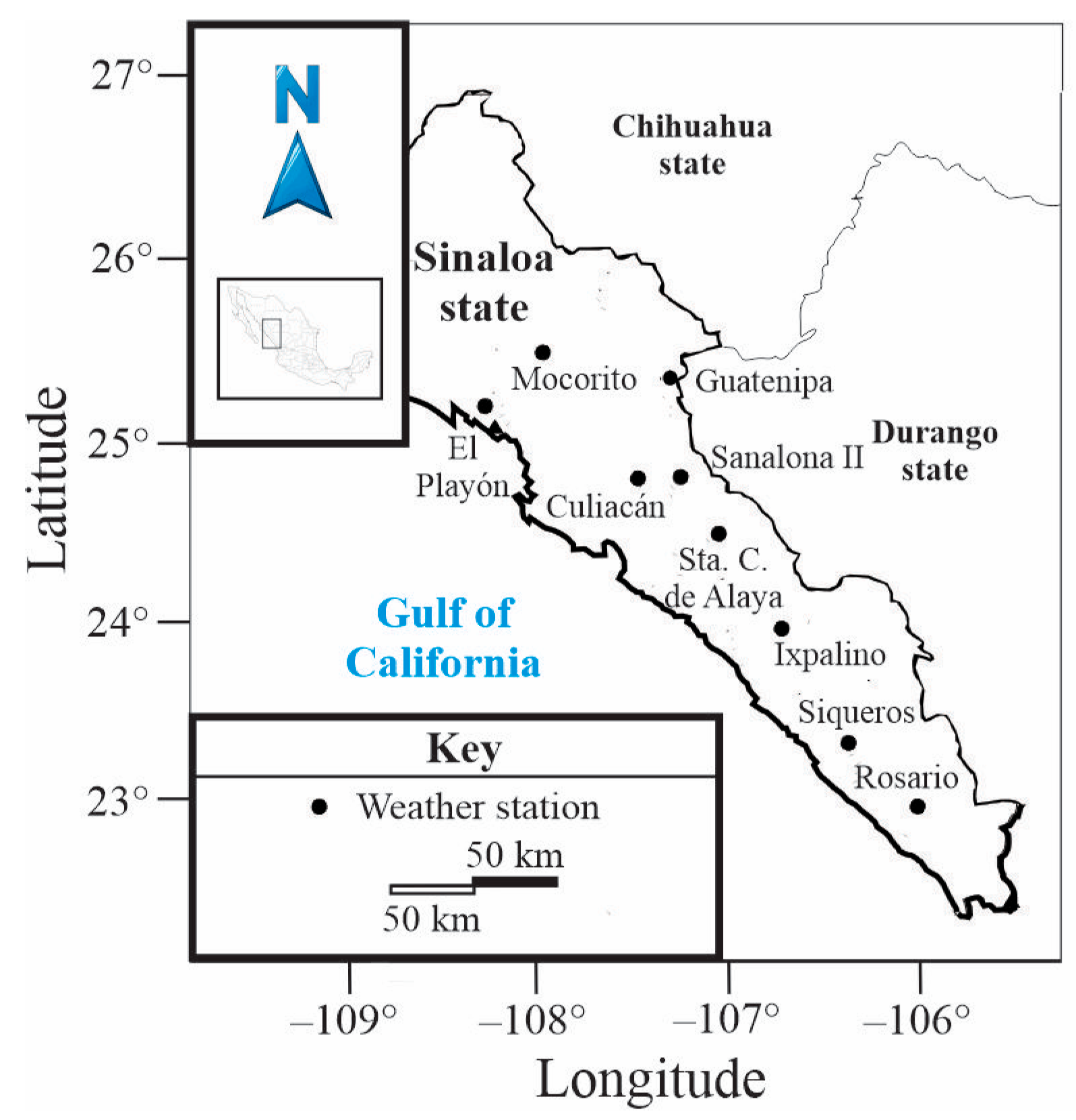
2.1. Study Area
2.2. Obtaining and Running Quality Control of Daily Rainfall (DaR) Data
2.3. Cumulative Annual Rainfall (CAR), Annual Average Rainfall (AAR), Seasonal Average Rainfall (SAR), Seasonal Cumulative Rainfall (SCR), and 99th Percentile (P99)
2.4. Temporal Variability of Intense Rainfall Erosivity Indices (IRE)
2.5. Spatial Variability—Trend of Observed Rainfall Erosivity Risk (ORE)
2.6. Predicted Rainfall Erosivity Risk (PRE)
2.7. Validation of Predicted Rainfall Erosivity Risk (PRE) Models
Normality Analysis of Residuals from Multiple Linear Regression (MLR)
2.8. Fitting Multiple Nonlinear Regressions (MNRs) Between Observed and Predicted Rainfall Erosivity Risk (ORE vs. PRE)
2.9. Simulation of Predicted Rainfall Erosivity Risk (PRE)
2.9.1. Cumulative Distribution Functions (CDFs)
2.9.2. Adjusted Return Periods (ARP)
2.10. Software Used and Significance of Statistical Analyses
3. Results
3.1. Maximum, 99th Percentile (P99), and Average Values of Cumulative Annual Rainfall (CAR), Annual Average Rainfall (AAR), Seasonal Average Rainfall (SAR), and Seasonal Cumulative Rainfall (SCR)
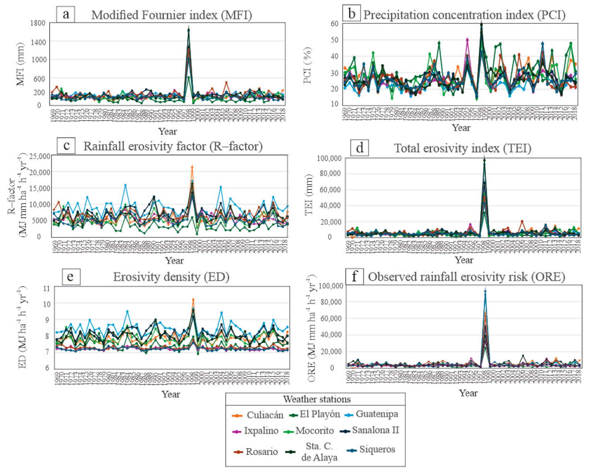
3.2. Intense Rainfall Erosivity (IRE) Indices
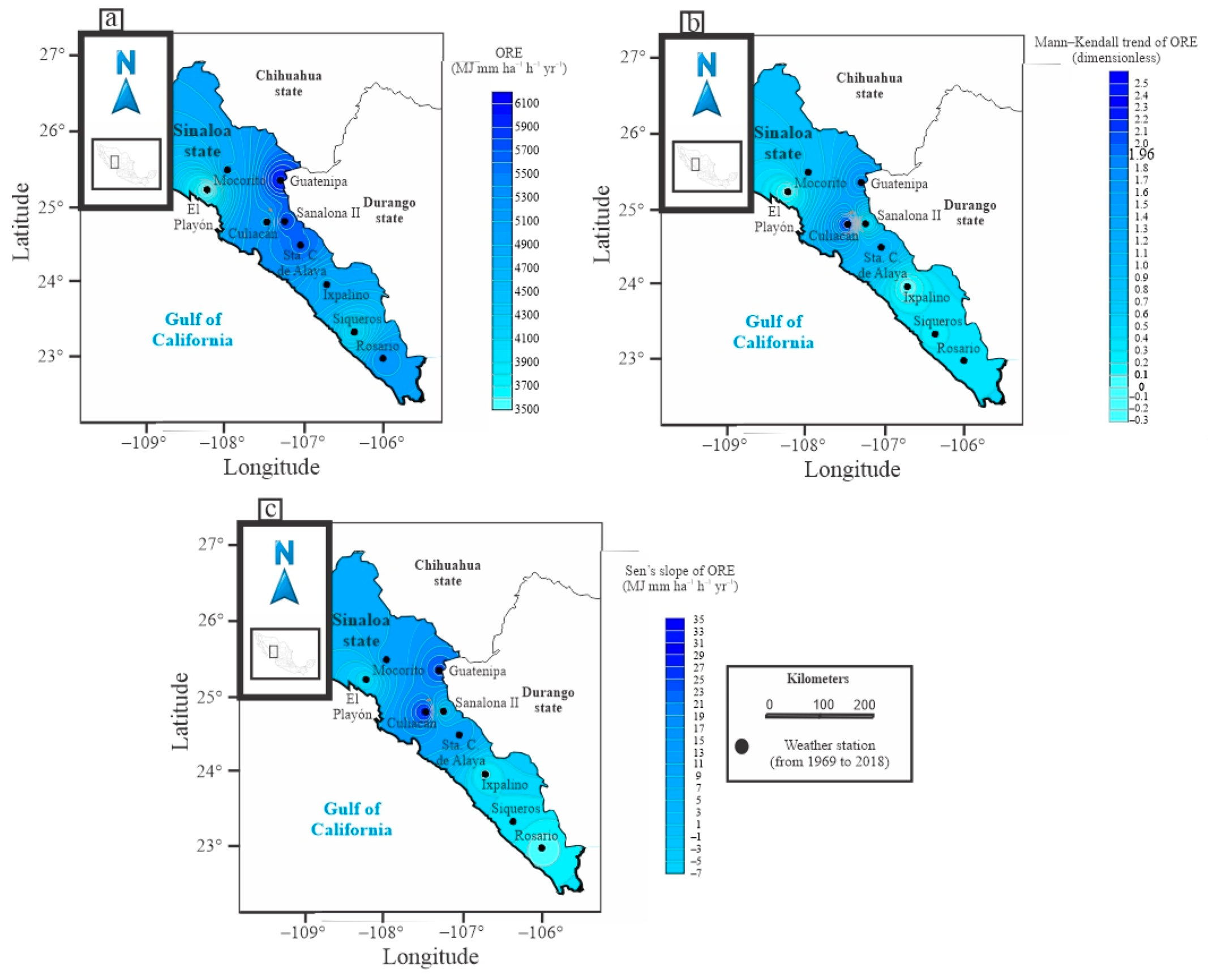
3.3. Spatial Variability—Trend of Observed Rainfall Erosivity Risk (ORE)
3.4. Validation of the Models of Predictive Rainfall Erosivity Risk (PRE)
Normality Analysis of the Residuals of Multiple Linear Regression (MLR)
3.5. Models of Predicted Rainfall Erosivity Risk (PRE)
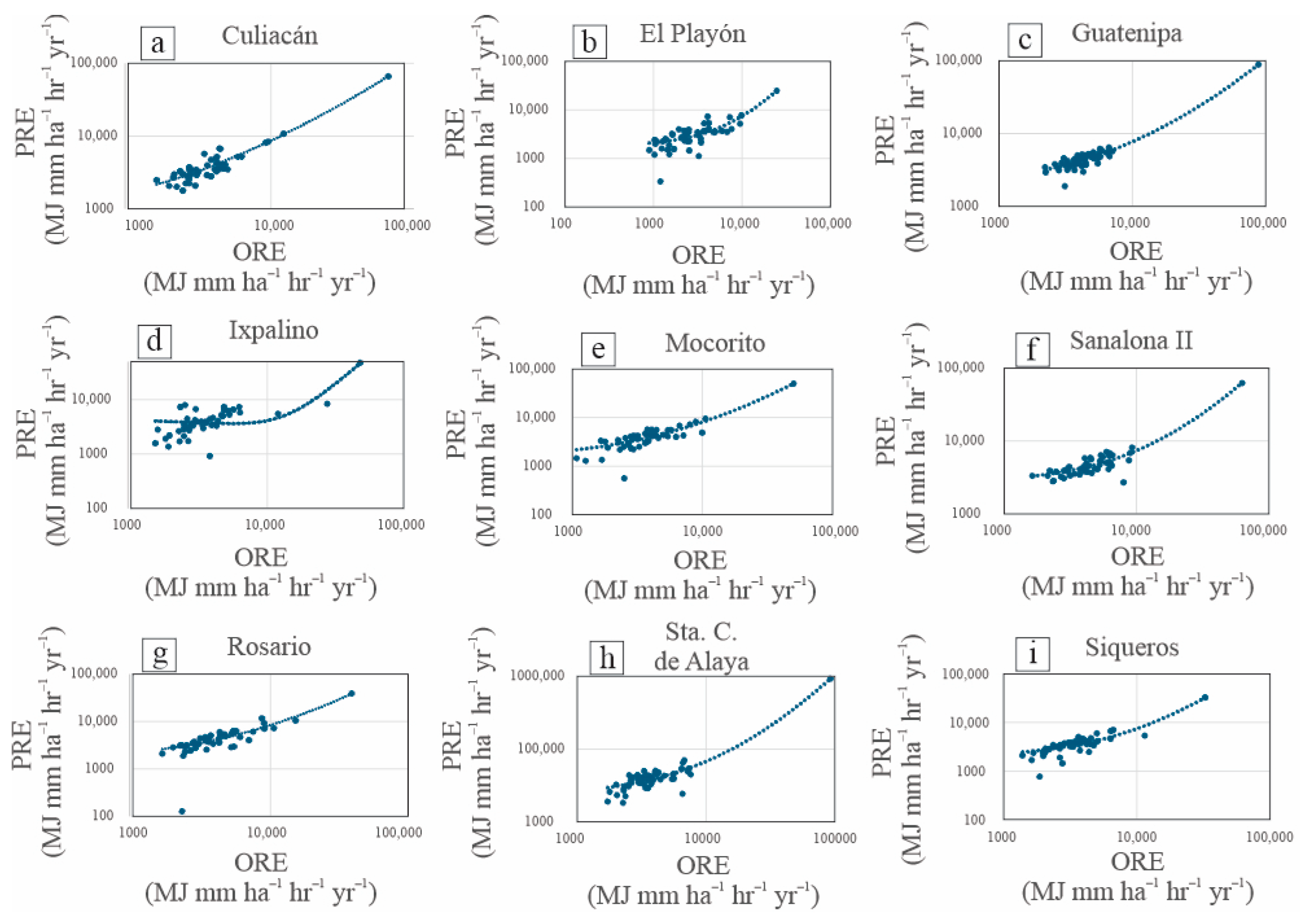
3.6. Fitting Multiple Nonlinear Regressions (MNRs) Between Observed and Predicted Rainfall Erosivity Risk (ORE vs. PRE)
3.7. Simulation of Predicted Rainfall Erosivity Risk (PRE)
p-Values of the Cumulative Distribution Functions (CDFs) That Recorded the Best Fit
3.8. Parameters of the Cumulative Distribution Functions (CDFs) That Recorded the Best Fit
3.9. Adjusted Return Periods (ARPs) of Cumulative Annual Rainfall (CAR), Annual Average Rainfall (AAR), Seasonal Average Rainfall (SAR) and Seasonal Cumulative Rainfall (SCR)
3.10. Application of Simulation and Adjusted Return Periods (ARPs) of Predicted Rainfall Erosivity Risk (PRE)
4. Discussion
5. Conclusions
Author Contributions
Funding
Institutional Review Board Statement
Informed Consent Statement
Data Availability Statement
Conflicts of Interest
Abbreviations
| IRE | Intense rainfall erosivity |
| MFI | Modified Fournier index |
| PCI | Precipitation concentration index |
| TEI | Total erosivity index |
| USLE | Universal soil loss equation |
| R-factor | Rainfall erosivity factor |
| ED | Erosivity density |
| CAR | Cumulative annual rainfall |
| AAR | Annual average rainfall |
| SAR | Seasonal average rainfall |
| SCR | Seasonal cumulative rainfall |
| CDF | Cumulative distribution function |
| Probability density function | |
| ARP | Adjusted return period |
| ORE | Observed rainfall erosivity risk |
| DaR | Daily rainfall |
| MLR | Multiple linear regression |
| MNR | Multiple nonlinear regression |
| PRE | Predicted rainfall erosivity risk |
| mR | Monthly cumulative rainfall |
| R2 | Determination coefficient |
| Sr | Spearman correlation coefficient |
| Scr | Spearman critical correlation coefficient |
| MRE | Mean relative error |
| RMSLE | Root mean square log error |
| P99 | 99th percentile |
References
- Fenta, A.A.; Tsunekawa, A.; Haregeweyn, N.; Yasuda, H.; Tsubo, M.; Borrelli, P.; Kawai, P.; Belay, S.A.; Ebabu, K.; Berihun, L.M.; et al. An integrated modeling approach for estimating monthly global rainfall erosivity. Sci. Rep. 2024, 14, 8167. [Google Scholar] [CrossRef]
- Dela, C.A.M.; Maniquiz, R.M.C.; Tanhueco, M.R.; De Leon, M. Estimation of the Rainfall Erosivity Factor (R-Factor) for Application in Soil Loss Models. Water 2025, 17, 837. [Google Scholar] [CrossRef]
- Pérez, C.P.; Benabdeluahab, S.; Salhi, A. Mitigating Erosion and Enhancing Sediment Retention: A Modeling Approach to Sustainable Land Management. Earth Syst. Environ. 2025, 9, 1–20. [Google Scholar] [CrossRef]
- Wei, P.; Du, J.; Bahadur, A.; Zhang, H.; Wang, S.; Wu, T.; Chen, S. Soil erosion and risk assessment on the Qinghai-Tibetan Plateau. Commun. Earth Environ. 2025, 6, 365. [Google Scholar] [CrossRef]
- Diodato, N.; Di Salvo, C.; Bellocchi, G. Climate driven generative time-varying model for improved decadal storm power predictions in the Mediterranean. Commun. Earth Environ. 2025, 6, 212. [Google Scholar] [CrossRef]
- Wischmeier, W.H.; Smith, D.D. Predicting rainfall erosion losses—A guide to conservation planning. In Agriculture Handbook; U.S. Department of Agriculture: Washington, DC, USA, 1978; p. 537. Available online: https://www.ars.usda.gov/ARSUserFiles/60600505/RUSLE/AH_537%20Predicting%20Rainfall%20Soil%20Losses.pdf (accessed on 6 January 2026).
- Knight, J.; Elbasit, A.M.A.M. Spatial and Temporal Patterns of Rainfall Erosivity in Southern Africa in Extreme Wet and Dry Years. Atmosphere 2024, 15, 1283. [Google Scholar] [CrossRef]
- Wang, L.; Li, Y.; Gan, Y.; Zhao, L.; Qin, W.; Ding, L. Rainfall erosivity index for monitoring global soil erosion. Catena 2024, 234, 107593. [Google Scholar] [CrossRef]
- Terefe, B.; Melese, T.; Tsegaye, A.; Afework, A.; Yibeltal, T.; Anagaw, A.; Temesgen, F.; Belay, T.; Assefa, G.; Bekele, M.B. Soil loss estimation in Ethiopia: A comprehensive review of the RUSLE model integrated with geospatial technologies. Discov. Sustain. 2025, 6, 334. [Google Scholar] [CrossRef]
- Husein, H.H.; Kalkha, M.; Baladia, R.; Al-Sarem, A.; Umler, B.; Sahwan, W.; Lucke, B. Soil erosion assessment in the rainy mountainous areas of the eastern Mediterranean. A case study of the El-Sarout watershed. Environ. Dev. Sustain. 2024, 1–26. [Google Scholar] [CrossRef]
- Fournier, J. Agressivité climatique et risques érosifs dans la region de Dschang Ouest Cameroun. Bull. Réseau Erosion 1994, 14, 145–156. Available online: https://beep.ird.fr/collect/bre/index/assoc/14-145-1.dir/14-145-156.pdf (accessed on 6 January 2026).
- Hernando, D.; Romana, G.M. Estimating the rainfall erosivity factor from monthly precipitation data in the Madrid Region (Spain). J. Hydrol. Hydromech. 2015, 63, 55–62. [Google Scholar] [CrossRef]
- Nasidi, M.N.; Wayayok, A.; Abdullah, F.A.; Kassim, M.S.M. Dynamics of potential precipitation under climate change scenarios at Cameron highlands, Malaysia. SN Appl. Sci. 2021, 3, 334. [Google Scholar] [CrossRef]
- Vargas, B.J.; Sáez, B.B. Analysis of aggressiveness rainfall in the far north of Chile. In Proceedings of the E-Proceedings of the 38th IAHR World Congress, Panama City, Panama, 1–6 September 2019; Available online: https://static.iahr.org/34/435.pdf (accessed on 6 January 2026).
- Llanes, C.O.; Norzagaray, C.M.; Pérez, G.E.; Gaxiola, A.; López, R.J.S.; González, G.G.E. Trend analysis and historical and recent return periods of erosivity indicators in the state of Sinaloa, Mexico. Arab. J. Geosci. 2020, 13, 212. [Google Scholar] [CrossRef]
- Yin, S.; Nearing, A.M.; Borrelli, P.; Xue, X. Rainfall Erosivity: An Overview of Methodologies and Applications. Vadose Zone J. 2017, 16, 12. [Google Scholar] [CrossRef]
- Koralay, N.; Kara, Ö. Risk assessment of soil erosion with RUSLE using geographic information system and organic carbon and total nitrogen loadings of suspended sediment in Sogutlu Stream Watershed of Trabzon, Turkey. Environ. Earth Sci. 2025, 84, 258. [Google Scholar] [CrossRef]
- Panagos, P.; Ballabio, C.; Borrelli, P.; Meusburger, K.; Klik, A.; Rousseva, S.; Perčec, T.M.; Michaelides, S.; Hrabalíková, M.; Olsen, P.; et al. Rainfall erosivity in Europe. Sci. Total Environ. 2015, 511, 801–814. [Google Scholar] [CrossRef] [PubMed]
- Panagos, P.; Borrelli, P.; Spinoni, J.; Ballabio, C.; Meusburger, K.; Beguería, S.; Klik, A.; Michaelides, S.; Petan, S.; Hrabalíková, M.; et al. Monthly Rainfall Erosivity: Conversion Factors for Different Time Resolutions and Regional Assessments. Water 2016, 8, 119. [Google Scholar] [CrossRef]
- Bai, Q.; Wang, L.; Cidan, Y. Spatial and Temporal Variability of Rainfall Erosivity in the Niyang River Basin. Atmosphere 2024, 15, 1032. [Google Scholar] [CrossRef]
- Meusburger, K.; Steel, A.; Panagos, P.; Montanarella, L.; Alewell, C. Spatial and temporal variability of rainfall erosivity factor for Switzerland. Hydrol. Earth Syst. Sci. 2012, 16, 167–177. [Google Scholar] [CrossRef]
- Lu, H.; Yu, B. Spatial and seasonal distribution of rainfall erosivity in Australia. Soil Res. 2002, 40, 6. [Google Scholar] [CrossRef]
- Xu, X.; Lyu, D.; Lei, X.; Huang, T.; Li, Y.; Yi, H.; Guo, J.; He, L.; He, J.; Yang, X.; et al. Variability of extreme precipitation and rainfall erosivity and their attenuated effects on sediment delivery from 1957 to 2018 on the Chinese Loess Plateau. J. Soils Sediments 2021, 21, 3933–3947. [Google Scholar] [CrossRef]
- Canavos, C.G. Probabilidad y Estadística: Aplicaciones y Métodos; McGraw-Hill: Columbus, OH, USA, 1988; p. 651. Available online: https://aulavirtual.agro.unlp.edu.ar/pluginfile.php/59208/mod_resource/content/0/Canavos_-_Probabilidad_y_estadistica_1998_-_PARTE_1.pdf (accessed on 6 January 2026).
- Kim, J.; Porter, J.; Kearns, E.J. Exposure of the US population to extreme precipitation risk has increased due to climate change. Sci. Rep. 2023, 13, 21782. [Google Scholar] [CrossRef]
- Pandit, D.V.; Isaac, R.K. A Scenario of Rainfall Erosivity Index Research. Int. J. Eng. Res. 2015, 4, 12. Available online: https://www.researchgate.net/publication/287149491_A_Scenario_of_Rainfall_Erosivity_Index_Research (accessed on 6 January 2026). [CrossRef]
- Gebremichael, A.; Gebremariam, E.; Desta, H. GIS-based mapping of flood hazard areas and soil erosion using analytic hierarchy process (AHP) and the universal soil loss equation (USLE) in the Awash River Basin, Ethiopia. Geosci. Lett. 2025, 12, 12. [Google Scholar] [CrossRef]
- Becerra, M.A. Erosión de Suelos; Universidad Autónoma Chapingo: Texcoco, Mexico, 1997. [Google Scholar]
- Montes, L.M.A.L.; Uribe, A.E.M.; García, C.E. Mapa nacional de erosion potencial. Tecnol. Cienc. Agua 2011, 2, 1. Available online: https://www.revistatyca.org.mx/index.php/tyca/article/view/223 (accessed on 6 January 2026).
- Servicio Meteorológico Nacional–Comisión Nacional del Agua (SMN–CONAGUA). Base de Datos Meteorológicos de México. Available online: https://smn.conagua.gob.mx/es/climatologia/informacion-climatologica/informacion-estadistica-climatologica (accessed on 12 February 2025).
- González, M.E.; Rolla, A.L.; Sánchez, M.V. Seasonal probabilistic precipitation prediction in Comahue region (Argentina) using statistical techniques. Theor. Appl. Climatol. 2022, 151, 1483–1495. [Google Scholar] [CrossRef]
- Ortiz, P.J.P.; Sandoval, S.S.; Arellano, G.J.; Medellín, A.J.; Edward, T.J. Managing Water Differently: Integrated Water Resources Management as a Framework for Adaptation to Climate Change in Mexico; Springer: Berlin/Heidelberg, Germany, 2020; Available online: https://link.springer.com/chapter/10.1007/978-3-030-16565-9_6 (accessed on 6 January 2026).
- Kraft, K.H.; Luna, R.J.J.; Gepts, P. A new collection of wild populations of Capsicum in Mexico and the southern United States. Genet. Resour. Crop. Evol. 2013, 60, 225–232. [Google Scholar] [CrossRef]
- Instituto Nacional de Estadística, Geografía e Informática (INEGI). Información Geoespacial de la Distribución de los Tipos de Suelos en México. 2025. Available online: https://www.inegi.org.mx/temas/edafologia/ (accessed on 6 January 2026).
- Guijarro, J.A.; López, J.A.; Aguilar, E.; Domonkos, P.; Venema, V.K.; Sigró, J.; Brunet, M. Homogenization of monthly series of temperature and precipitation: Benchmarking results of the MULTITEST project. Int. J. Climatol. 2023, 43, 9. [Google Scholar] [CrossRef]
- Abubakar, H.B.; Scholes, M.C.; Engelbrecht, F.A. Spatio-temporal trends in daily precipitation extremes over the Enkangala escarpment of South Africa: 1961–2021. Theor. Appl. Climatol. 2025, 156, 164. [Google Scholar] [CrossRef]
- Yin, S.; Xie, Y.; Liu, B.; Nearing, M.A. Rainfall erosivity estimation based on rainfall data collected over a range of temporal resolutions. Hydrol. Earth Syst. Sci. 2015, 19, 4113–4126. Available online: http://www.hydrol-earth-syst-sci.net/19/4113/2015/ (accessed on 6 January 2026). [CrossRef]
- Salameh, A.M.A. Using the precipitation concentration index for characterizing the rainfall distribution in the Levant. J. Water Clim. Chang. 2024, 15, 4. [Google Scholar] [CrossRef]
- Arnoldus, H.M.J. An Approximation of the Rainfall Factor in the Universal Soil Loss Equation. In Assessment of Erosion; De Boodt, M., Gabriels, D., Eds.; John Wiley and Sons: Hoboken, NJ, USA, 1980; pp. 127–132. [Google Scholar]
- Pereira, C.D.; Marcelino, S.E.; Cesar, A.J.; Augusto, M.J.; Furtado, F.D.; Naves, S.M.L.; Acuña, G.S.F.; Curi, N. Rainfall erosivity factor: An R package for rainfall erosivity (R-factor) determination. Catena 2020, 189, 104509. [Google Scholar] [CrossRef]
- Cortés, T.H.G. Caracterización de la Erosividad de la Lluvia en México Utilizando Métodos Multivariados. Master’s Thesis, Centro de Edafología, Colegio de Postgraduados, Montecillo, Mexico, 1991; p. 168. [Google Scholar]
- Mancilla, V.O.R. Diseño y Evaluación de Terrazas de Banco Para Plantaciones Forestales Comerciales. Master’s Thesis, Colegio de Postgraduados, Montecillo, Mexico, 2008; p. 95. Available online: http://colposdigital.colpos.mx:8080/xmlui/handle/10521/1422 (accessed on 6 January 2026).
- Vega, M.B.; Febles, J.M. La agresividad de la lluvia en áreas rurales de la provincia de La Habana como factor de presión en la sostenibilidad agroambiental. In Proceedings of the II Seminario Internacional de Cooperación y Desarrollo en Espacios Rurales Iberoamericanos, Sostenibilidad e Indicadores, Almería, Spain, 14–16 December 2008. [Google Scholar]
- Castelán, V.R.; Tamariz, F.V.; Linares, F.G.; Cruz, M.A. Agresividad de las precipitaciones en la subcuenca del río San Marcos, Puebla, México. Investig. Geog. 2014, 83, 28–40. [Google Scholar] [CrossRef]
- Kinnell, P.I.A. Event soil loss, runoff and the Universal Soil Loss Equation family of models: A review. J. Hydrol. 2010, 385, 384–397. [Google Scholar] [CrossRef]
- Ghosh, A.; Bhattacharjee, S.; Bera, B. Hydro-Geomorphological mapping of Manbhum Singhbhum plateau (Part of Singhbhum protocontinent, India) for water resource development and land use planning. J. Indian Soc. Remote Sens. 2023, 51, 8. [Google Scholar] [CrossRef]
- Giri, S.; Kumar, T.A.; Kumar, M.M.; Kumar, S.A. Major ion chemistry and suitability of groundwater resources for different utilizations in mica mining areas, Jharkhand, India. Geochem. Trans. 2025, 26, 5. [Google Scholar] [CrossRef] [PubMed]
- Tuğrul, T.; Oruç, S.; Hınıs, A.M. Analyzing temperature trends using innovative trend analyses in certain regions of Norway. Acta Geophys. 2025, 73, 4883–4902. [Google Scholar] [CrossRef]
- Bhargav, K.K.; Sharma, S.; Bhowmik, D.R.; Mujumdar, P.P. Spatial synchronization of river floods growing beyond the basin boundaries in Peninsular India. Sci. Rep. 2025, 15, 18160. [Google Scholar] [CrossRef] [PubMed]
- Llanes, C.O.; Estrella, G.R.D.; Parra, G.R.E.; Gutiérrez, R.O.G.; Ávila, D.J.A.; Troyo, D.E. Modeling Yield of Irrigated and Rainfed Bean in Central and Southern Sinaloa State, Mexico, Based on Essential Climate Variables. Atmosphere 2024, 15, 573. [Google Scholar] [CrossRef]
- Méndez, M.; Magaña, V. Regional Aspects of Prolonged Meteorological Droughts over Mexico and Central America. J. Clim. 2010, 23, 5. [Google Scholar] [CrossRef]
- Farfán, M.L.; Romero, C.R.; Raga, B.G. Observations and Forecasts from the Landfall of Tropical Cyclones John, Lane, and Paul (2006) over Northwestern Mexico. Weather. Forecast. 2012, 27, 6. [Google Scholar] [CrossRef]
- Farfán, M.L.; D’sa, J.E.; Liu, K.; Rivera, M.V.H. Tropical Cyclone Impacts on Coastal Regions: The Case of the Yucatán and the Baja California Peninsulas, Mexico. Estuaries Coasts 2014, 37, 1388–1402. [Google Scholar] [CrossRef]
- Vega, C.J.P.; Brito, C.L. Precipitation response in mountainous and coastal regions of Northwestern Mexico under ENSO scenarios during the landfall of tropical cyclones. Theor. Appl. Climatol. 2024, 155, 8599–8610. [Google Scholar] [CrossRef]
- Nanko, K.; Moskalski, M.S.; Torres, R. Rainfall erosivity–intensity relationships for normal rainfall events and a tropical cyclone on the US southeast coast. J. Hydrol. 2016, 534, 440–450. [Google Scholar] [CrossRef]
- Das, S.; Jain, J.M.; Gupta, V.; McGehee, P.R.; Yin, S.; de Mello, R.C.; Azaris, M.; Borelli, P.; Panagos, P. GloRESatE: A dataset for global rainfall erosivity derived from multi-source data. Sci. Data 2024, 11, 926. [Google Scholar] [CrossRef]
- Botai, C.M.; Botai, J.O.; Mukhawana, M.B.; Wit, J.; Masilela, N.S.; Zwane, N.; Tazvinga, H. Evaluation of rainfall distribution based on the precipitation concentration index: A case study over the selected summer rainfall regions of South Africa. Hydrology 2025, 12, 136. [Google Scholar] [CrossRef]
- Wang, G.; Hu, H.; Islam, A.R.M.T.; Akter, Y.; Fattah, A.; Kabir, Z.; Hasan, G.; Islam, A.; Arabameri, A.; Chandra, P.S.; et al. Spatiotemporal rainfall concentration and erosivity in a tropical monsoon country. Theor. Appl. Climatol. 2025, 156, 251. [Google Scholar] [CrossRef]
- Das, S.; Kumar, J.M.; Auerswald, K.; de Mello, C.R.; Molnar, P. Identifyng monthly rainfall erosivity patterns using hourly rainfall data across India. Sci. Rep. 2025, 15, 27940. [Google Scholar] [CrossRef]
- Kokoska, S.; Nevison, C. Critical Values for Spearman’s Rank Correlation Coefficient. In Statistical Tables and Formulae; Springer Texts in Statistics; Springer: New York, NY, USA, 1989. [Google Scholar] [CrossRef]
- Yang, C.W.; Yang, Y.J.; Kim, C.R. Multiple Quadratic Polynomial Regression Models and Quality Mapsfor Tensile Mechanical Properties and Quality Indices of Cast Aluminum Alloys according to Artificial Aging Heat Treatment Condition. Adv. Mater. Sci. Eng. 2023, 2023, 7069987. [Google Scholar] [CrossRef]
- Jadon, A.; Patil, A.; Jadon, S. A Comprehensive Survey of Regression-Based Loss Functions for Time Series Forecasting. In Data Management, Analytics and Innovation. ICDMAI 2024. Lecture Notes in Networks and Systems; Sharma, N., Goje, A.C., Chakrabarti, A., Bruckstein, A.M., Eds.; Springer: Singapore, 2024; Volume 998, Available online: https://link.springer.com/chapter/10.1007/978-981-97-3245-6_9#citeas (accessed on 6 January 2026).
- Papacharalampous, G.; Tyralis, H.; Koutsoyiannis, D. Predictability of monthly temperature and precipitation using automatic time series forecasting methods. Acta Geophys. 2018, 66, 807–831. Available online: https://link.springer.com/article/10.1007/s11600-018-0120-7 (accessed on 6 January 2026). [CrossRef]
- Gupta, D.; Kundu, D. Generalized Logistic Distributions. J. Appl. Stat. Sci. 2010, 18, 1. Available online: https://www.researchgate.net/publication/228882269_Generalized_Logistic_Distributions (accessed on 6 January 2026).
- Chagnaud, G.; Panthou, G.; Vischel, T.; Blanchet, J.; Lebel, T. A unified statistical framework for detecting trends in multi-timescale precipitation extremes: Application to non-stationary intensity-duration-frequency curves. Theor. Appl. Climatol. 2021, 145, 839–860. [Google Scholar] [CrossRef]
- Osetinsky, T.I.; Fredj, E. The 50- and 100-year Exceedance Probabilities as New and Convenient Statistics for a Frequency Analysis of Extreme Events: An Example of Extreme Precipitation in Israel. Water 2022, 15, 44. [Google Scholar] [CrossRef]
- Maity, S.S.; Maity, R. Changing Pattern of Intensity–Duration–Frequency Relationship of Precipitation due to Climate Change. Water Resour. Manag. 2022, 36, 5371–5399. [Google Scholar] [CrossRef]
- Ng, L.J.; Huang, F.Y.; Yong, S.L.; Lee, C.J.; Ahmed, N.A.; Mirzaei, M. Analysing the variability of non-stationary extreme rainfall events amidst climate change in East Malaysia. Aqua Water Infrastruct. Ecosyst. Soc. 2024, 73, 7. [Google Scholar] [CrossRef]
- Mohamed, J.; Ali, A.A.; Warsame, A.A.; Adam, B.M. Two phases of long-term shift in extreme precipitation in Somalia. Meteorol. Atmos. Phys. 2022, 134, 54. [Google Scholar] [CrossRef]
- Mínguez, R.; Herrera, S. Spatial extreme model for rainfall depth: Application to the estimation of IDF curves in the Basque country. Sthoch. Environ. Res. Risk Assess. 2023, 37, 3117–3148. [Google Scholar] [CrossRef]
- Aihaiti, A.; Wang, Y.; Ali, M.; Zhu, L.; Liu, J.; Zhang, H.; Gao, J.; Wen, C.; Song, M. Probability distribution characteristics of summer extreme precipitation in Xinjiang, China during 1970–2021. Theor. Appl. Climatol. 2023, 151, 753–766. [Google Scholar] [CrossRef]
- Naderi, M.; Ardeh, F.T.; Abedi, F.; Masoumi, Z. Impact of land-use and climate change on future extreme flows: A study for three dam watersheds in Alborz and Tehran provinces of Iran. Appl. Water Sci. 2025, 15, 49. [Google Scholar] [CrossRef]
- Johannsen, L.L.; Schmaltz, M.E.; Mitrovits, O.; Klik, A.; Smoliner, W.; Wang, S.; Strauss, P. An update of the spatial and temporal variability of rainfall erosivity (R-factor) for the main agricultural production zones of Austria. Catena 2022, 215, 106305. [Google Scholar] [CrossRef]
- Fotiadis, A.; Vlachos, I.; Kugiumtzis, D. Detecting Nonlinear Interactions in Complex Systems: Application in Financial Markets. Entropy 2023, 25, 370. [Google Scholar] [CrossRef] [PubMed]
- Zhou, W.; Yan, Z.; Zhang, L. A comparative study of 11 non-linear regression models highlighting autoencoder, DBN, and SVR, enhanced by SHAP importance analysis in soybean branching prediction. Sci. Rep. 2024, 14, 5905. [Google Scholar] [CrossRef] [PubMed]
- Flores, C.L.M.; Ramírez, S.M.; Osorio, P.A. Repercusiones del cambio climático global en el estado de Sinaloa. Cuad. Geogr. Rev. Colomb. Geogr. 2012, 21, 1. Available online: http://ref.scielo.org/8qrpyg (accessed on 6 January 2026).




| Rainfall Erosivity Index | |
|---|---|
| (1) | |
| (2) | |
| (3) | |
| (4) | |
| (5) | |
| (6) | |
| (7) | |
| (8) |
| Variable Name | Mathematical Equations Used to Calculate Probability Density Functions (PDFs), Cumulative Distribution Functions (CDFs), and Adjusted Return Periods (ARPs) | |
|---|---|---|
| Log-normal (x; μ, σ) | (9) | |
| (10) | ||
| (11) | ||
| (12) | ||
| (13) | ||
| (14) | ||
| Cumulative distribution function (CDF) | ; where f(x) and f(z) are the probability density functions (PDFs) | (15) |
| Adjusted return period (ARP) | (16) | |
| Variable | Inferential Statistic | Rainfall Amount (mm yr−1) Weather Station | ||||||||
|---|---|---|---|---|---|---|---|---|---|---|
| Culiacán | El Playón | Guatenipa | Ixpalino | Mocorito | Rosario | Sanalona II | Sta. C. de Alaya | Siqueros | ||
| CAR | Maximum | 2088.20 | 881.30 | 1766.80 | 1617.60 | 1494.30 | 1975.10 | 1471.20 | 1707.10 | 1613.60 |
| P99 | 1588.94 | 850.92 | 1720.50 | 1381.52 | 1329.32 | 1423.97 | 1703.79 | 1529.97 | 1376.98 | |
| Average | 699.36 | 463.03 | 1040.62 | 790.94 | 705.86 | 930.35 | 872.08 | 775.63 | 743.38 | |
| AAR | Maximum | 89.11 | 73.44 | 139.36 | 94.65 | 96.47 | 118.45 | 114.57 | 112.13 | 94.23 |
| P99 | 84.32 | 70.91 | 137.42 | 94.09 | 94.16 | 107.43 | 117.92 | 102.69 | 92.56 | |
| Average | 55.74 | 37.95 | 85.00 | 64.52 | 57.57 | 76.11 | 71.31 | 62.91 | 60.78 | |
| SAR | Maximum | 277.13 | 231.03 | 332.73 | 305.13 | 296.10 | 403.83 | 328.47 | 334.60 | 293.03 |
| P99 | 267.40 | 220.37 | 331.77 | 287.31 | 283.31 | 321.31 | 385.08 | 331.19 | 288.67 | |
| Average | 174.02 | 109.13 | 238.77 | 189.03 | 175.69 | 231.94 | 220.69 | 189.48 | 186.12 | |
| SCR | Maximum | 831.40 | 693.10 | 998.20 | 915.40 | 888.30 | 1211.50 | 985.40 | 1003.80 | 879.10 |
| P99 | 802.20 | 661.10 | 995.31 | 861.94 | 849.93 | 963.45 | 1155.25 | 993.56 | 866.01 | |
| Average | 522.05 | 327.38 | 716.30 | 567.08 | 527.07 | 695.82 | 662.08 | 568.43 | 558.35 | |
| Observed Rainfall Erosivity Risk Index (ORE, MJ mm ha−1 h−1 yr−1) | Category | Index Value |
|---|---|---|
| 0–5000 | Very low | 1 |
| 5001–10,000 | Low | 2 |
| 10,001–15,000 | Medium | 3 |
| 15,001–20,000 | High | 4 |
| >20,000 | Very high | 5 |
| N/Weather Station | p-Value (Dimensionless) | ||||||||
|---|---|---|---|---|---|---|---|---|---|
| Culiacán | El Playón | Guatenipa | Ixpalino | Mocorito | Sanalona II | Rosario | Sta. C. de Alaya | Siqueros | |
| Shapiro–Wilk W | 0.944 | 0.932 | 0.932 | 0.459 | 0.902 | 0.872 | 0.841 | 0.873 | 0.704 |
| p (normal) | 0.019 | 0.007 | 0.007 | 0.000 | 0.001 | 0.000 | 0.000 | 0.000 | 0.000 |
| Anderson–Darling A | 0.796 | 1.241 | 1.007 | 7.556 | 1.264 | 1.492 | 2.368 | 2.122 | 3.125 |
| p (normal) | 0.036 | 0.003 | 0.011 | 0.000 | 0.002 | 0.001 | 0.000 | 0.000 | 0.000 |
| p (Monte Carlo) | 0.036 | 0.002 | 0.009 | 0.000 | 0.003 | 0.001 | 0.000 | 0.000 | 0.000 |
| Jarque–Bera JB | 17.700 | 8.313 | 10.900 | 1925.000 | 20.450 | 63.790 | 52.500 | 26.190 | 471.900 |
| p (normal) | 0.000 | 0.016 | 0.004 | 0.000 | 0.000 | 0.000 | 0.000 | 0.000 | 0.000 |
| p (Monte Carlo) | 0.004 | 0.023 | 0.013 | 0.000 | 0.004 | 0.001 | 0.001 | 0.002 | 0.000 |
| Weather Station | MRE (%) | RMSLE (Dimensionless) | R2 (Dimensionless) | Sr (Dimensionless) |
|---|---|---|---|---|
| Culiacán | 20.457 | 0.100 | 0.992 | 0.996 |
| El Playón | 40.640 | 0.205 | 0.898 | 0.948 |
| Guatenipa | 16.412 | 0.087 | 0.997 | 0.998 |
| Ixpalino | 36.048 | 0.198 | 0.894 | 0.946 |
| Mocorito | 24.500 | 0.151 | 0.978 | 0.989 |
| Sanalona II | 22.265 | 0.126 | 0.988 | 0.994 |
| Rosario | 23.211 | 0.209 | 0.948 | 0.974 |
| Sta. C. de Alaya | 22.898 | 0.123 | 0.997 | 0.998 |
| Siqueros | 21.991 | 0.127 | 0.955 | 0.977 |
| Weather Station | Log-Normal | Normal | GEV | Gamma (2) | Beta4 | Logistic |
|---|---|---|---|---|---|---|
| Maximum p-Value (Dimensionless) | ||||||
| Culiacán | SCR = 1.00 SAR = 1.00 CAR = 0.96 | AAR = 1.00 | ||||
| El Playón | AAR = 0.97 | SCR = 0.99 SAR = 0.99 CAR = 0.99 | ||||
| Guatenipa | AAR = 0.98 SAR = 0.90 SCR = 0.90 | CAR = 0.96 | ||||
| Ixpalino | AAR = 0.98 | CAR = 1.00 SAR = 0.99 SCR = 0.99 | ||||
| Mocorito | CAR = 0.96 | SAR = 0.96 | AAR = 0.98 | SCR = 0.96 | ||
| Sanalona II | AAR = 0.89 SAR = 0.84 SCR = 0.84 | CAR = 0.94 | ||||
| Rosario | CAR = 0.62 AAR = 0.84 | SAR = 0.97 SCR = 0.98 | ||||
| Sta. C. de Alaya | AAR = 0.87 | CAR = 0.85 | SAR = 0.77 SCR = 0.77 | |||
| Siqueros | CAR = 0.97 AAR = 0.95 SAR = 1.00 SCR = 1.00 | |||||
| Weather Station | Parameters of Cumulative Distribution Functions (CDFs) | |||||
|---|---|---|---|---|---|---|
| Log-Normal | Normal | GEV | Gamma (2) | Beta4 | Logistic | |
| Culiacán | SCR ( = 6.24; = 0.21) SAR ( = 5.14; = 0.21) CAR ( = 6.51; = 0.28) | AAR ( = 1.86, = 3.44, c = 32.08, and d = 99.44) | ||||
| El Playón | AAR ( = 3.57; = 0.39) | SCR ( = 6.36; = 51.46) SAR ( = 6.36 = 17.15) CAR ( = 6.96; = 66.53) | ||||
| Guatenipa | SCR ( = 6.56; = 0.19) SAR ( = 5.46; = 0.19) AAR ( = 4.42; = 0.21) | CAR ( = −0.05, = 198.89, and = 930.73) | ||||
| Ixpalino | AAR ( = 4.14; = 0.23) | SCR ( = 3.39, = 10.01, c = 322.66, and d = 1289.52) SAR ( = 3.99, = 14.96, c = 103.83, and d = 508.10) CAR ( = 1.98, = 10.63, c = 456.90, and d = 2592.85) | ||||
| Mocorito | CAR ( = 6.52; = 0.28) | SAR ( = 175.69; = 44.66) | AAR ( = 15.74; = 3.66) | SCR ( = 25.72, = 28.63, c = −417.42, and d = 1579.81) | ||
| Sanalona II | SCR ( = 6.47; = 0.21) SAR ( = 5.38; = 0.21) AAR ( = 4.24; = 0.23) | CAR ( = −0.09, = 180.90, and = 775.51) | ||||
| Rosario | AAR ( = −0.01, = 12.95, and = 68.67) CAR ( = 0.10, = 191.77, and = 819.65) | SCR ( = 3.11, = 12.46, c = 349.52, and d = 2086.65) SAR ( = 3.51, = 17.75, c = 113.05, and d = 834.01) | ||||
| Sta. C. de Alaya | AAR ( = −0.05, = −0.10, and = 14.30) | CAR ( = 12.04; = 64.42) | SCR ( = 562.12; = 68.04) SAR ( = 187.38; = 22.68) | |||
| Siqueros | SCR ( = 6.29; = 0.27) SAR ( = 5.19; = 0.27) AAR ( = 4.08; = 0.24) CAR ( = 6.57; = 0.27) | |||||
| Weather Station | CAR (mm yr−1) | ARP (Years) | AAR (mm yr−1) | ARP (Years) | SAR (mm yr−1) | ARP (Years) | SCR (mm yr−1) | ARP (Years) | Weather Station | CAR (mm yr−1) | ARP (Years) | AAR (mm yr−1) | ARP (Years) | SAR (mm yr−1) | ARP (Years) | SCR (mm yr−1) | ARP (Years) |
|---|---|---|---|---|---|---|---|---|---|---|---|---|---|---|---|---|---|
| Culiacán | 300 | 1.00 | 40 | 1.12 | 150 | 1.37 | 450 | 1.37 | Sanalona II | 650 | 1.16 | 40 | 1.01 | 150 | 1.04 | 600 | 1.56 |
| 600 | 1.53 | 50 | 1.60 | 180 | 2.54 | 550 | 2.78 | 850 | 2.08 | 60 | 1.35 | 200 | 1.56 | 700 | 2.81 | ||
| 900 | 6.94 | 60 | 2.82 | 210 | 6.46 | 650 | 8.23 | 1050 | 5.62 | 80 | 3.73 | 250 | 4.13 | 800 | 6.37 | ||
| 1200 | 55.05 | 70 | 6.53 | 240 | 20.76 | 750 | 31.86 | 1250 | 20.34 | 100 | 18.11 | 300 | 17.13 | 900 | 17.13 | ||
| 1500 | 523.55 | 80 | 23.67 | 270 | 78.43 | 850 | 146.92 | 1450 | 93.46 | 120 | 120.62 | 350 | 94.08 | 1000 | 52.12 | ||
| El Playón | 200 | 1.04 | 20 | 1.08 | 50 | 1.06 | 100 | 1.01 | Rosario | 800 | 1.49 | 60 | 1.17 | 200 | 1.48 | 500 | 1.12 |
| 400 | 1.67 | 40 | 2.67 | 100 | 1.88 | 300 | 1.88 | 1100 | 4.45 | 80 | 2.94 | 250 | 2.99 | 700 | 2.27 | ||
| 600 | 4.98 | 60 | 11.74 | 150 | 6.09 | 500 | 9.94 | 1400 | 14.72 | 100 | 12.11 | 300 | 8.08 | 900 | 7.93 | ||
| 800 | 22.80 | 80 | 58.34 | 200 | 29.47 | 700 | 97.86 | 1700 | 45.13 | 120 | 57.89 | 350 | 28.52 | 1100 | 46.73 | ||
| 1000 | 138.73 | 100 | 284.38 | 250 | 184.58 | 900 | 1380.83 | 2000 | 125.49 | 140 | 292.47 | 400 | 131.41 | 1300 | 514.87 | ||
| Guatenipa | 600 | 1.01 | 30 | 1.00 | 150 | 1.01 | 300 | 1.00 | Sta. C. de Alaya | 500 | 1.10 | 40 | 1.06 | 100 | 1.02 | 200 | 1.00 |
| 900 | 1.45 | 60 | 1.07 | 200 | 1.25 | 500 | 1.04 | 700 | 1.67 | 60 | 1.90 | 150 | 1.19 | 400 | 1.09 | ||
| 1200 | 4.57 | 90 | 2.83 | 250 | 2.71 | 700 | 1.96 | 900 | 3.76 | 80 | 6.87 | 200 | 2.74 | 600 | 2.74 | ||
| 1500 | 22.09 | 120 | 23.48 | 300 | 10.11 | 900 | 10.11 | 1100 | 11.95 | 100 | 41.01 | 250 | 16.82 | 800 | 33.99 | ||
| 1800 | 133.12 | 150 | 351.43 | 350 | 55.04 | 1000 | 30.29 | 1300 | 49.82 | 120 | 397.73 | 300 | 144.41 | 1000 | 624.62 | ||
| Ixpalino | 550 | 1.10 | 55 | 1.38 | 120 | 1.01 | 450 | 1.17 | Siqueros | 400 | 1.02 | 55 | 1.63 | 60 | 1.00 | 250 | 1.00 |
| 750 | 1.98 | 65 | 2.26 | 170 | 1.51 | 550 | 1.93 | 700 | 1.87 | 65 | 2.89 | 120 | 1.07 | 450 | 1.33 | ||
| 950 | 4.81 | 75 | 4.61 | 220 | 5.11 | 650 | 4.53 | 1000 | 9.40 | 75 | 6.15 | 180 | 2.01 | 650 | 4.13 | ||
| 1150 | 14.94 | 85 | 11.09 | 270 | 37.24 | 750 | 15.23 | 1300 | 76.87 | 85 | 14.87 | 240 | 7.16 | 850 | 22.59 | ||
| 1350 | 59.88 | 95 | 30.03 | 320 | 642.58 | 850 | 78.71 | 1600 | 744.02 | 95 | 39.34 | 300 | 36.23 | 1050 | 158.42 | ||
| Mocorito | 400 | 1.03 | 50 | 1.48 | 100 | 1.05 | 200 | 1.01 | |||||||||
| 600 | 1.49 | 60 | 2.49 | 150 | 1.39 | 400 | 1.21 | ||||||||||
| 800 | 3.62 | 70 | 5.32 | 200 | 3.41 | 600 | 3.38 | ||||||||||
| 1000 | 12.36 | 80 | 13.94 | 250 | 20.81 | 800 | 46.78 | ||||||||||
| 1200 | 50.33 | 90 | 43.56 | 300 | 372.22 | 1000 | 7070.50 |
Disclaimer/Publisher’s Note: The statements, opinions and data contained in all publications are solely those of the individual author(s) and contributor(s) and not of MDPI and/or the editor(s). MDPI and/or the editor(s) disclaim responsibility for any injury to people or property resulting from any ideas, methods, instructions or products referred to in the content. |
© 2026 by the authors. Licensee MDPI, Basel, Switzerland. This article is an open access article distributed under the terms and conditions of the Creative Commons Attribution (CC BY) license.
Share and Cite
González González, G.E.; Cárdenas, O.L.; Campos, M.N.; García Serrano, L.A.; Parra Galaviz, R.E.; Ávila Díaz, J.A.; Arciniega Galaviz, M.A. Variability, Prediction, and Simulation of Rainfall Erosivity Risk in the State of Sinaloa, Northwest Mexico. Atmosphere 2026, 17, 80. https://doi.org/10.3390/atmos17010080
González González GE, Cárdenas OL, Campos MN, García Serrano LA, Parra Galaviz RE, Ávila Díaz JA, Arciniega Galaviz MA. Variability, Prediction, and Simulation of Rainfall Erosivity Risk in the State of Sinaloa, Northwest Mexico. Atmosphere. 2026; 17(1):80. https://doi.org/10.3390/atmos17010080
Chicago/Turabian StyleGonzález González, Gabriel E., Omar Llanes Cárdenas, Mariano Norzagaray Campos, Luz A. García Serrano, Román E. Parra Galaviz, Jeován A. Ávila Díaz, and Marco A. Arciniega Galaviz. 2026. "Variability, Prediction, and Simulation of Rainfall Erosivity Risk in the State of Sinaloa, Northwest Mexico" Atmosphere 17, no. 1: 80. https://doi.org/10.3390/atmos17010080
APA StyleGonzález González, G. E., Cárdenas, O. L., Campos, M. N., García Serrano, L. A., Parra Galaviz, R. E., Ávila Díaz, J. A., & Arciniega Galaviz, M. A. (2026). Variability, Prediction, and Simulation of Rainfall Erosivity Risk in the State of Sinaloa, Northwest Mexico. Atmosphere, 17(1), 80. https://doi.org/10.3390/atmos17010080