A Short-Term Forecasting Model of Ionospheric hmF2 Based on Wavelet Transform and a Neural Network in China

Abstract

The peak height of the ionospheric F2 layer (hmF2) is a critical parameter in ionospheric physics and high-frequency radio wave propagation research. This study presents a backpropagation neural network (BPNN) enhanced by wavelet transform (WT) decomposition for one-hour-ahead hmF2 forecasting. The WT method decomposes and reconstructs the hmF2 time series, preserving its primary structural characteristics. Subsequently, the BPNN provides high-accuracy predictions. The model is trained and evaluated using 2014 hmF2 measurements from four observation stations in China. Utilizing only hmF2 data, the model produces accurate one-hour-ahead forecasts. The predicted values closely align with observed diurnal variations and exhibit lower fluctuations than those of the IRI and standalone BPNN models. On the test set, the proposed model achieves an average RMSE of 17.16 km, which is 10.10 km and 8.39 km lower than the IRI and BPNN models, respectively. The average RRMSE is 5.72%, representing reductions of 2.88% and 2.64% compared to the IRI and BPNN models, respectively. These findings indicate that the hybrid model is well-suited for the Chinese region and substantially enhances short-term hmF2 forecast accuracy.

1. Introduction

The ionosphere, which comprises the outer ionized region of the Earth’s atmosphere, is strongly influenced by solar and geomagnetic activity. Due to the complex dynamics of space plasma, the ionosphere exhibits random, nonlinear variations in both time and space [1]. Vertically, the ionosphere is divided into several layers based on changes in ionization levels or ion density. Notably, the F2 layer has the highest ion concentration, making it crucial for radio communication systems such as satellite, high-frequency, and radar communications [2]. As one of the important reference quantities for characterization of this layer, the peak height of the ionospheric F2 layer (hmF2) denotes the altitude corresponding to the maximum electron density in the ionosphere [3]. As a key parameter, hmF2 not only reflects variabilities caused by geomagnetic disturbances and solar activity but also provides valuable insight for deriving mid-latitude neutral winds [4]. Given these roles, an accurate forecast of hmF2 is vital for advancing research on the space environment and improving wireless communication systems.

Over the past several decades, researchers worldwide have employed a variety of methods to predict hmF2, including the time correlation function method [5], empirical orthogonal function analysis [6], neural network [7], and machine learning [8]. The International Reference Ionosphere (IRI) model [4,9], jointly developed by multiple international organizations, is an empirical ionospheric model constructed from globally distributed ionosonde and satellite observations. It has demonstrated strong long-term forecasting capability on a global scale and is widely used for long-term hmF2 prediction. In particular, its forecast performance has been validated in regions such as East Asia [10] and Southeast Asia [11]. For long-term hmF2 forecasting, Gulyaeva investigated the relationship between hmF2 and NmF2 during ionospheric storms and developed an empirical storm-time hmF2 model based on satellite observations [12]. Huang et al. [13] developed empirical models for foF2 and hmF2 based on ionosonde, reanalysis, and Constellation Observing System for Meteorology, Ionosphere, and Climate data. These models provide a more accurate representation of foF2 variations. Wang et al. [14] proposed a long-term prediction model grounded in ionospheric ray propagation theory, achieving higher accuracy than the IRI model. Li et al. [15] optimized artificial neural network (ANN) parameters using a genetic algorithm and established a global hmF2 forecasting model, which has demonstrated excellent performance in both global and regional ionospheric spatiotemporal prediction tasks. Compared with long-term forecasts, short-term and near–real-time hmF2 forecasts are more critical for capturing the rapidly varying ionospheric environment. Iban et al. [16] demonstrated that machine learning models exhibit strong forecast performance for hourly variations of foF2, hmF2, and TEC. Shi et al. [17] developed a hybrid deep learning model optimized using an improved Seagull Optimization Algorithm, achieving high-accuracy short-term hmF2 forecasts and demonstrating robust forecasting capability up to 48 h ahead. Hu et al. [3] applied a BI-LSTM model to the hmF2 forecast over Australia, noting that the model performs well with small training samples, converges quickly, and yields high forecasting accuracy. Rao et al. [18] used a BiLSTM model to forecast foF2 and hmF2 at a low-latitude station in Hyderabad, India, and found that the model maintained strong performance even during geomagnetic storm conditions. These studies collectively show that neural networks and deep learning models offer significant advantages in hmF2 forecasting. However, deep learning approaches typically require substantial computational resources, and preprocessing sample datasets and post-processing forecasts are crucial for achieving optimal performance. Therefore, it remains necessary to effectively process hmF2 datasets and design improved neural network architectures to further enhance the convergence speed and forecast accuracy of hmF2 short-term forecasting.

To further enhance the accuracy and computational efficiency of hmF2 forecasting, this paper proposes a hybrid approach that integrates the wavelet transform with a BPNN. The wavelet transform is employed to address the nonlinear and nonstationary characteristics of hmF2, while the BPNN model is used to achieve accurate short-term forecasting for 1 h. The remainder of this paper is organized as follows: Section 2 describes the dataset and the data partitioning strategy. Section 3 introduces the wavelet transform and BPNN methods and outlines the detailed implementation of the proposed approach. Section 4 presents the forecasting experiments, compares the proposed model with benchmark methods, and analyzes its forecast performance. Section 5 concludes the paper.

2. Data

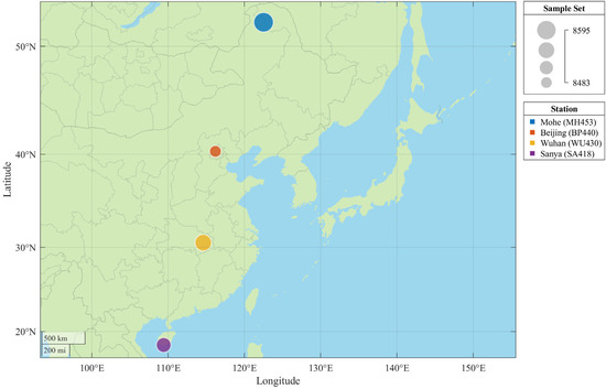
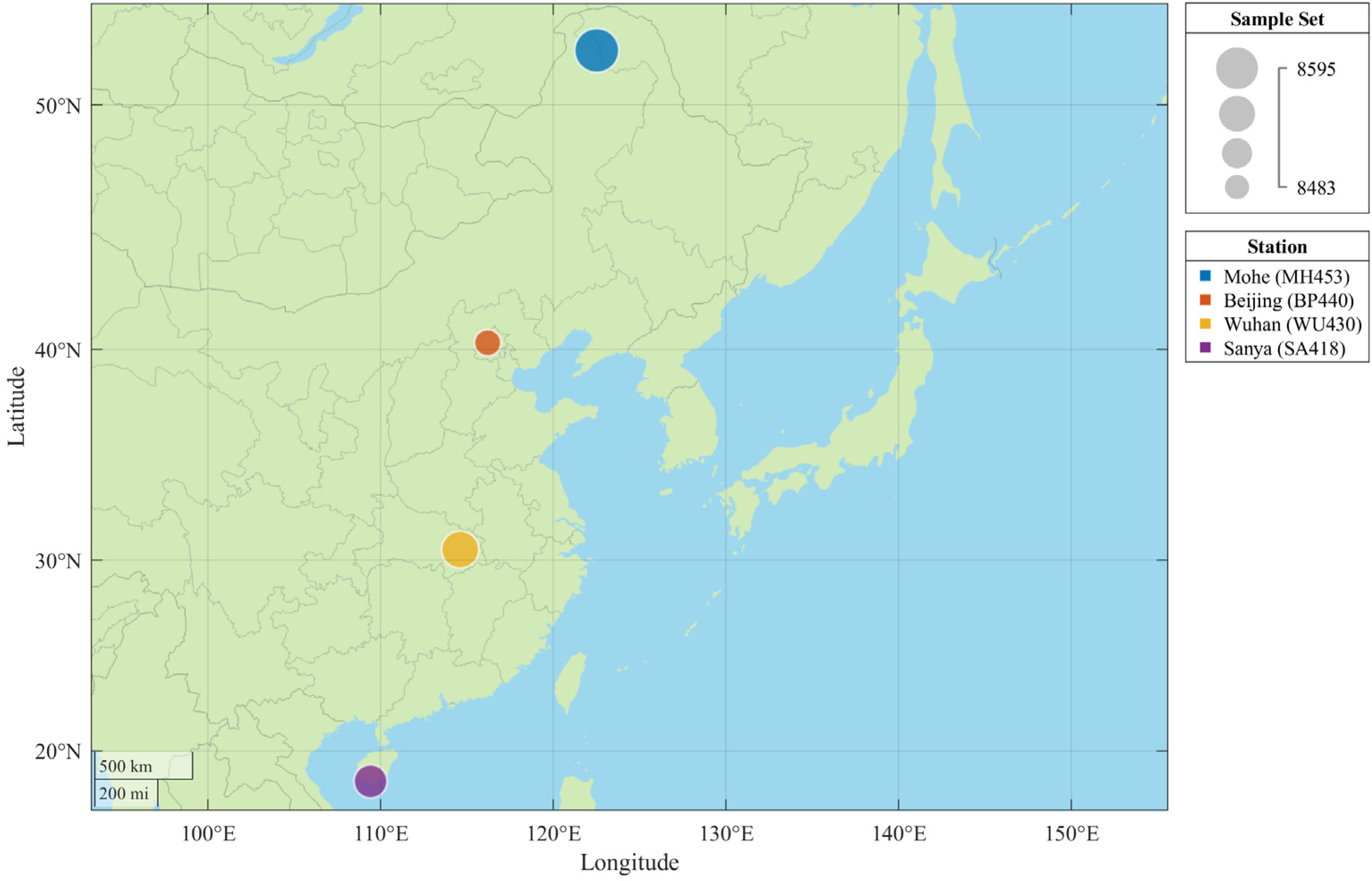
This study uses hmF2 vertical sounding data collected in 2014 from four ionospheric observation stations in China, spanning high, middle, and low latitudes. From north to south, the stations are Mohe (52.00° N, 122.52° E), Beijing (40.30° N, 116.20° E), Wuhan (30.50° N, 114.40° E), and Sanya (18.34° N, 109.42° E). These stations represent typical ionospheric characteristics at high, mid-, and low latitudes, enabling an evaluation of the model’s forecasting performance across different latitude regions. The geographic distribution of the stations is shown in Figure 1. Mohe is located at the northernmost point of China, Beijing and Wuhan lie in the mid-latitude region, and Sanya is situated in the southernmost part of China, within the low-latitude equatorial zone. Hourly hmF2 observations from these stations were obtained from the National Earth System Science Data Center (NESSDC) website (https://geospace.geodata.cn/data, accessed on 10 May 2024). The hmF2 values provided are manually measured and generally of high quality; however, some data gaps remain due to instrument limitations and other factors.

Table 1. Data availability of four ionospheric observation stations.

Stations	URSI Code	Latitude (° N)	Longitude (° E)	Data Availability (%)
Mohe	MH453	52.00	122.52	98.12
Beijing	BP440	40.30	116.20	96.84
Wuhan	WU430	30.53	114.61	97.55
Sanya	SA418	18.34	109.42	97.24

presents the data validity and specific coordinates for the four stations. The data validity for all stations exceeds 96%, indicating a high level of reliability, although some data are missing. To address this issue and recover missing values as fully as possible, we supplemented the dataset with additional measurements from NESSDC and the Global Ionospheric Radio Observatory (GIRO) database (https://giro.uml.edu/didbase/scaled.php, accessed on 12 May 2024).

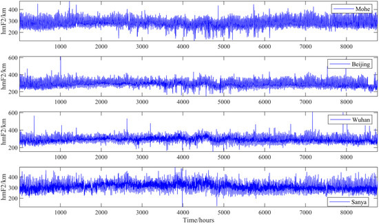
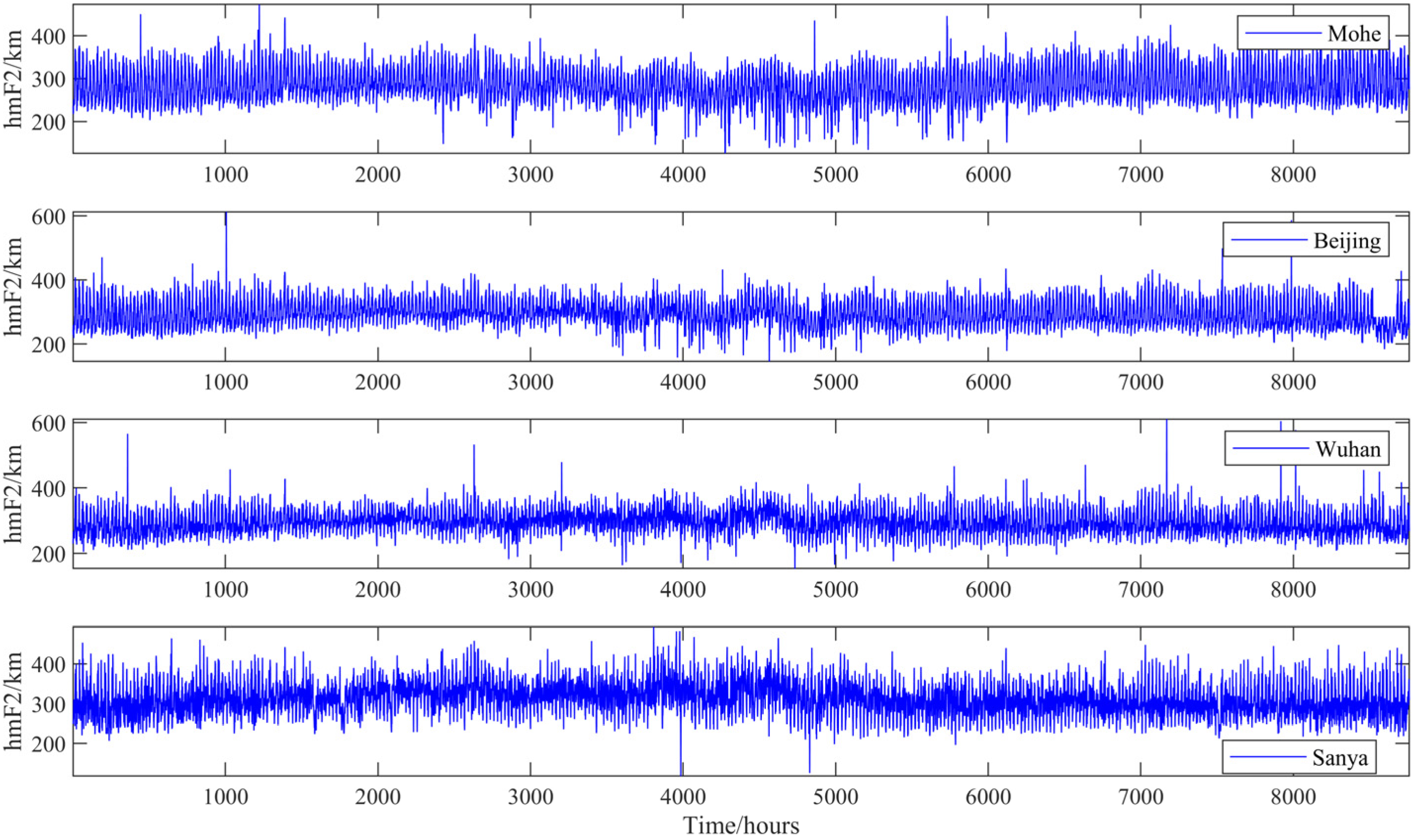
Using the methods described above, we obtained a relatively comprehensive dataset; however, outliers and missing values remained. IRI is an internationally recognized ionospheric model, and research results indicate that it performs well at multiple stations in China [19]. To address this, the remaining missing hmF2 values were filled with IRI-predicted values, yielding a continuous hmF2 dataset. A complete, high-quality dataset provides reliable input for the forecasting model and improves forecast accuracy. In addition, zero-mean normalization was applied to standardize the sample data, which accelerated neural network convergence and enhanced the model’s generalization capability. In this study, the hmF2 data from the four stations were partitioned into training and test sets in a 6:4 ratio. Figure 2 shows the preprocessed hmF2 data for all stations in 2014. It can be observed that certain time periods still contain noticeable noise, indicating the need for appropriate denoising techniques to further improve the model’s forecast performance.

3. Methods

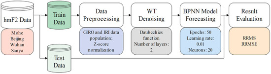
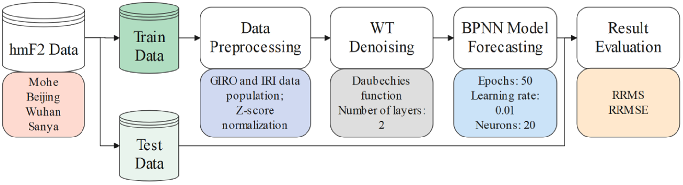
Given the nonlinear and unstable characteristics of hmF2, the wavelet transform is applied to denoise the preprocessed hmF2 time series prior to forecasting with a BPNN, as illustrated in Figure 3. First, the dataset is partitioned into training and test sets using a 6:4 ratio. The dataset is then supplemented with GIRO and IRI models’ prediction values, followed by normalization to enhance the usability and stability of the sample set. Next, the wavelet transform is employed to denoise the processed data, thereby further improving data quality. A BPNN model is subsequently used to rapidly forecast short-term variations in hmF2. Finally, the model’s forecast performance is evaluated on the test set.

3.1. Wavelet Transform

The wavelet transform (WT) algorithm [20] is highly effective for extracting key features from signals. While it inherits the localization concept of the short-time Fourier transform, it also introduces significant advancements that address several limitations of traditional Fourier-based methods. In particular, the window function of the wavelet transform varies with time, giving the method strong adaptability and making it well suited for tasks such as feature extraction, pattern recognition, and signal denoising. Wavelet transforms can be categorized into continuous and discrete forms. Because hmF2 is an hourly time-series dataset with finite length, this study employs the discrete wavelet transform to process the data. The discrete wavelet transform is defined as:

$$W{T}_{\mathrm{y}}\left(j,n\right)={{\alpha }_0}^{-{\displaystyle \frac{j}{2}}}{\displaystyle \int y\left(x\right){\psi }^{\ast }}\left({{\alpha }_0}^{-j}t-n{\tau }_0\right)dt$$

(1)

where, $\alpha$ is the scaling parameter; $\tau$ is the translation parameter; ${\psi }^{\ast }\left(x\right)$ is the complex conjugate function; j is the scaling parameter (representing the number of decompositions); n is the translation constant; and j and n are both integers.

Discrete wavelet decomposition facilitates multi-scale analysis of the original signal by separating it into high-frequency and low-frequency components, which is particularly beneficial for denoising time series data. The Mallat algorithm [21], a fast discrete orthogonal wavelet transform, is utilized to decompose and reconstruct the nonlinear hmF2 time series. The decomposition process is outlined below:

$$a_j=B{a}_{j-1},d_j=C{a}_{j-1},j=1,2,\dots N$$

(2)

where B and C are low-pass and high-pass filters, respectively; $a_j$ and $d_j$ represent low-frequency and high-frequency information, respectively; N is the maximum number of decomposition layers.

The Mallat algorithm decomposes the original chaotic time series into low-frequency approximation components and high-frequency detail components. The approximation components capture the overall trends and fundamental characteristics of the time series, whereas the detail components represent dynamic perturbations and transient fluctuations. The decomposed time series may subsequently be reconstructed using the Mallat algorithm as described below:

$$a_{j-1}=B^{\ast }{a}_j+C^{\ast }{d}_j,j=1,2,\dots N$$

(3)

where, $B^{\ast }$ and $C^{\ast }$ are the dual operators of B and C, respectively. After decomposing the original sequence s(t) according to Formula (3), the decomposition of each level and the expression of s(t) can be obtained as follows [22]:

$$s\left(t\right)=a_0=a_N+d_1+\dots +d_N$$

(4)

This study utilizes the discrete wavelet transform to decompose and reconstruct the hmF2 time series for denoising. The reconstructed data are subsequently used to train a BPNN, thereby reducing forecast errors and enhancing the accuracy of hmF2 predictions. The Daubechies (Db) wavelet is selected for its advantageous time–frequency localization and compact support, making it suitable for non-stationary time series. This wavelet effectively manages signal processing and mitigates boundary effects associated with fixed support length. Although Db wavelets are generally orthogonal, they often lack symmetry. As the order N increases, wavelet regularity improves, but computational cost also rises. Experimental evaluation indicates that the Db4 wavelet is optimal for decomposing and reconstructing the ionospheric hmF2 time series. The number of decomposition levels depends on the signal-to-noise ratio (SNR) of the input data. For high SNR signals, where the input primarily reflects time series information, excessive decomposition is unnecessary. In contrast, for noisy input signals, additional decomposition levels are advantageous [23]. In this study, the number of decomposition layers is set to two to balance real-time performance with forecast accuracy.

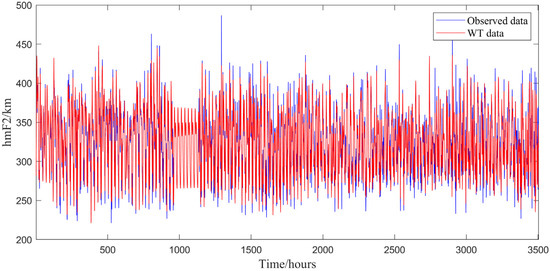
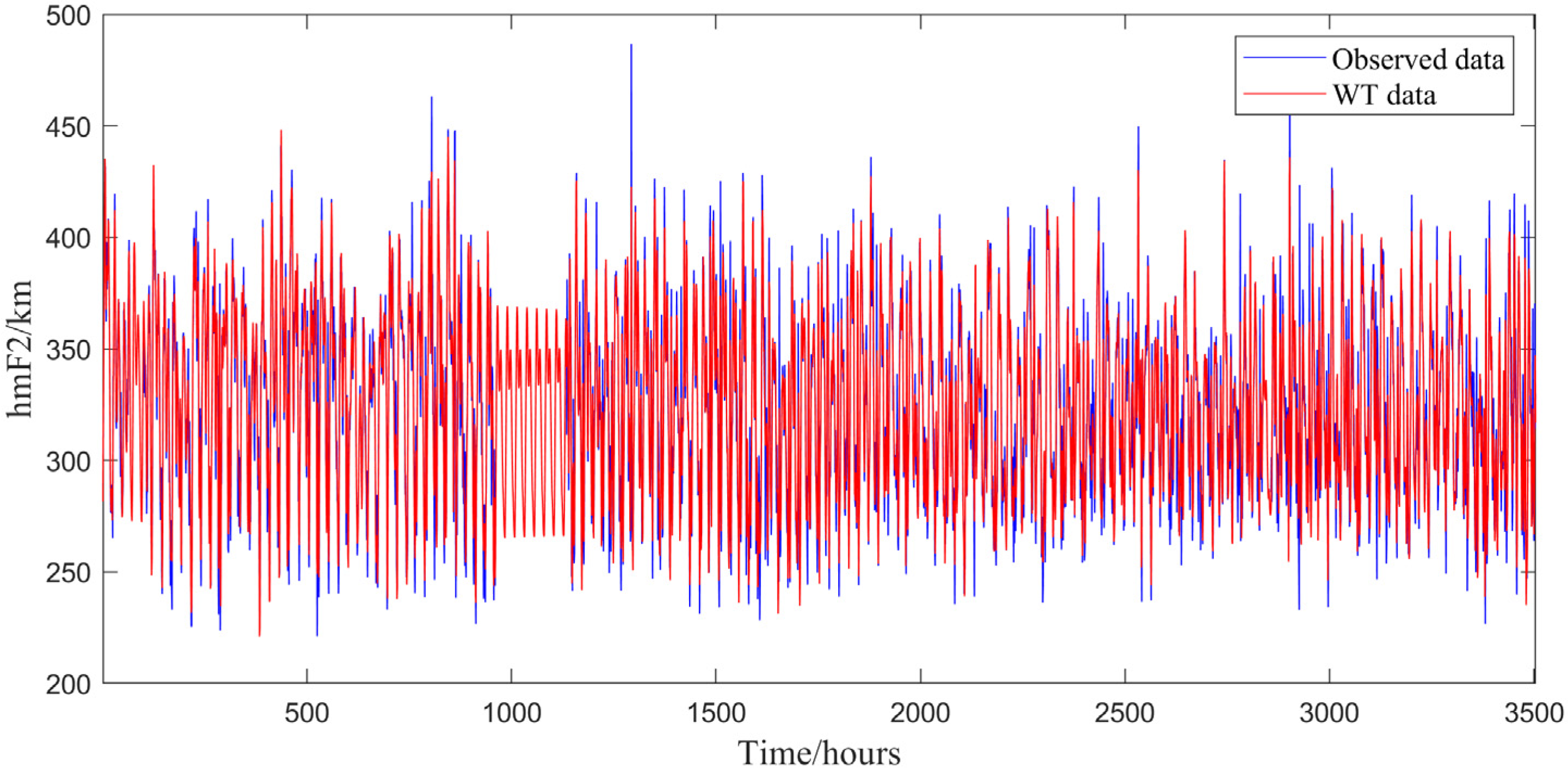
Figure 4 presents the denoised hmF2 data from the 2014 test set at the Sanya station. The WT algorithm effectively reduces noise. Blank regions in Figure 4 represent missing data points, which are managed using the data preprocessing procedures described previously.

3.2. Backpropagation Neural Network

The backpropagation neural network (BPNN) is a type of feedforward neural network trained with the backpropagation algorithm [24]. Training consists of two steps: first, the input is processed through the network to produce an output; second, the difference between the output and the target value is propagated backwards through the network. This error is used to update the network’s weights and biases, typically via gradient descent, to minimize the error and align the model’s output more closely with the expected result.

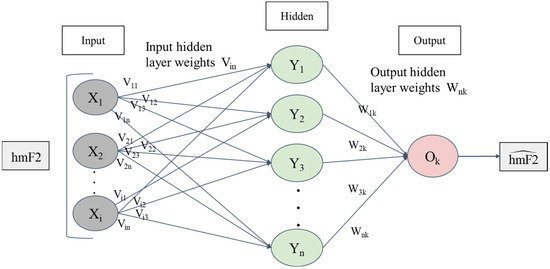
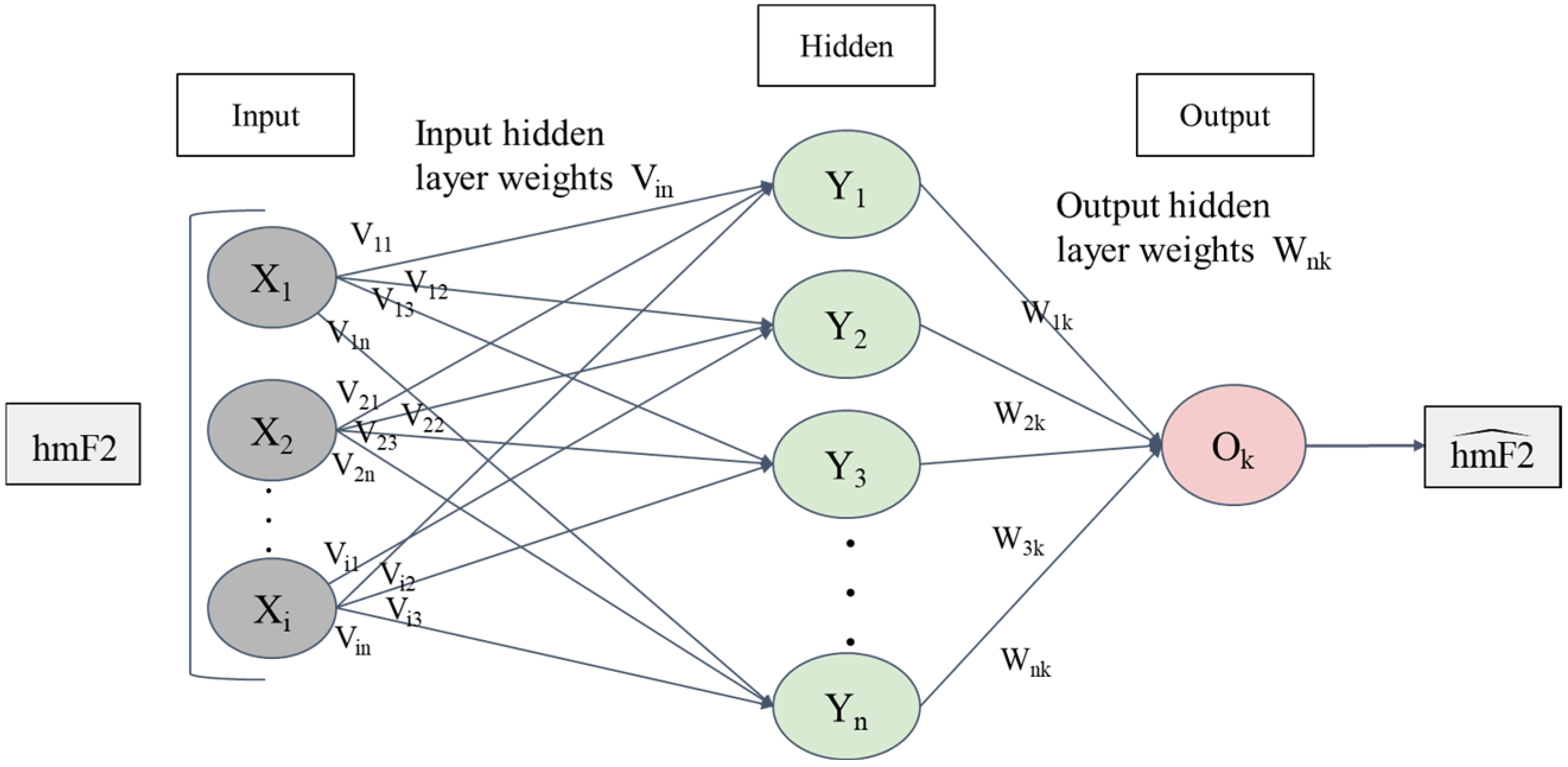
As shown in Figure 5, BPNN employs a classic feedforward topology, consisting of an input layer, one or more hidden layers, and an output layer, all interconnected via full connections. The neuron output from one layer feeds into the next, facilitating a powerful mechanism for nonlinear feature mapping. This capability is particularly advantageous for modeling systems with complex underlying dynamics. The hmF2 time series, governed by the stochastic evolution of the ionosphere, possesses pronounced spatiotemporal characteristics leading to inherent nonlinear and nonstationary behavior [17]. The BPNN’s inherent ability for self-learning and adaptive feature extraction enables the efficient storage and processing of the data’s complex characteristics through the network’s adjustable weights. Consequently, a BPNN neural network is deployed herein to develop a forecast model for the hmF2 parameter, thereby improving the model’s capacity to handle dynamic ionospheric information. Prior applications of the BPNN algorithm to ionospheric parameter forecast can be found in the research by Habarulema and McKinnell [25]. This article uses the following BPNN model hyperparameters: 20 neurons, 50 training epochs, and a learning rate of 0.01.

3.3. Evaluation Metrics

In the analysis of forecast accuracy in this article, missing data are excluded from the statistical analysis to avoid the impact of imputation on forecast accuracy. Error quantification and forecast accuracy validation for the proposed model utilize two primary statistical measures: Root Mean Square Error (RMSE) and Relative Root Mean Square Error (RRMSE). Model effectiveness increases as the values of these metrics decrease; specifically, lower RMSE and RRMSE values correspond to higher forecast accuracy. The formulas for these error metrics are presented below:

$$RMSE=\sqrt{{\displaystyle \frac{1}{N}}{\displaystyle \sum _{j=1}^N{\left(H_{obs}^j-H_{for}^j\right)}^2}}$$

(5)

$$RRMSE=\sqrt{{\displaystyle \frac{1}{N}}{\displaystyle \sum _{j=1}^N{\left(\frac{H_{obs}^j-H_{for}^j}{H_{obs}^j}\right)}^2}}\times 100$$

(6)

where, $H_{obs}^j$ represents the j-th actual observation in the hmF2 time series, $H_{for}^j$ represents the j-th forecasted value, and N is the length of the time series.

4. Results and Discussion

Randomly initializing model parameters may affect prediction accuracy. In this study, the model was trained 20 times using the training sets from the four stations, and its forecasting performance was statistically analyzed on the corresponding test sets.

Table 2. The WT-BPNN model forecasting result statistics.

Metrics	Statistic	Mohe	Beijing	Wuhan	Sanya
RMSE (km)	Max	13.56	17.30	25.65	27.49
	Min	13.01	15.22	19.33	17.71
	Mean	13.29	16.10	21.40	20.03
RRMSE (%)	Max	4.96	5.90	8.66	8.69
	Min	4.77	4.97	6.18	5.66
	Mean	4.88	5.37	6.99	6.45

presents the forecasting statistics of the WT-BPNN model at each station, including the maximum, minimum, and mean RMSE and RRMSE values from the 20 runs. The results in Table 2 indicate that the model demonstrates the smallest variation in evaluation metrics at the Mohe station and the largest variation at the Sanya station. This pattern suggests that variability in forecasting performance decreases progressively with increasing latitude. To reduce the impact of randomness in model parameter initialization, a set of forecast outputs near the mean was selected for detailed performance analysis.

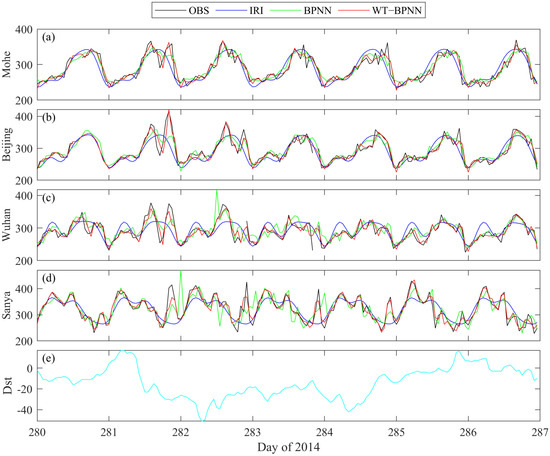
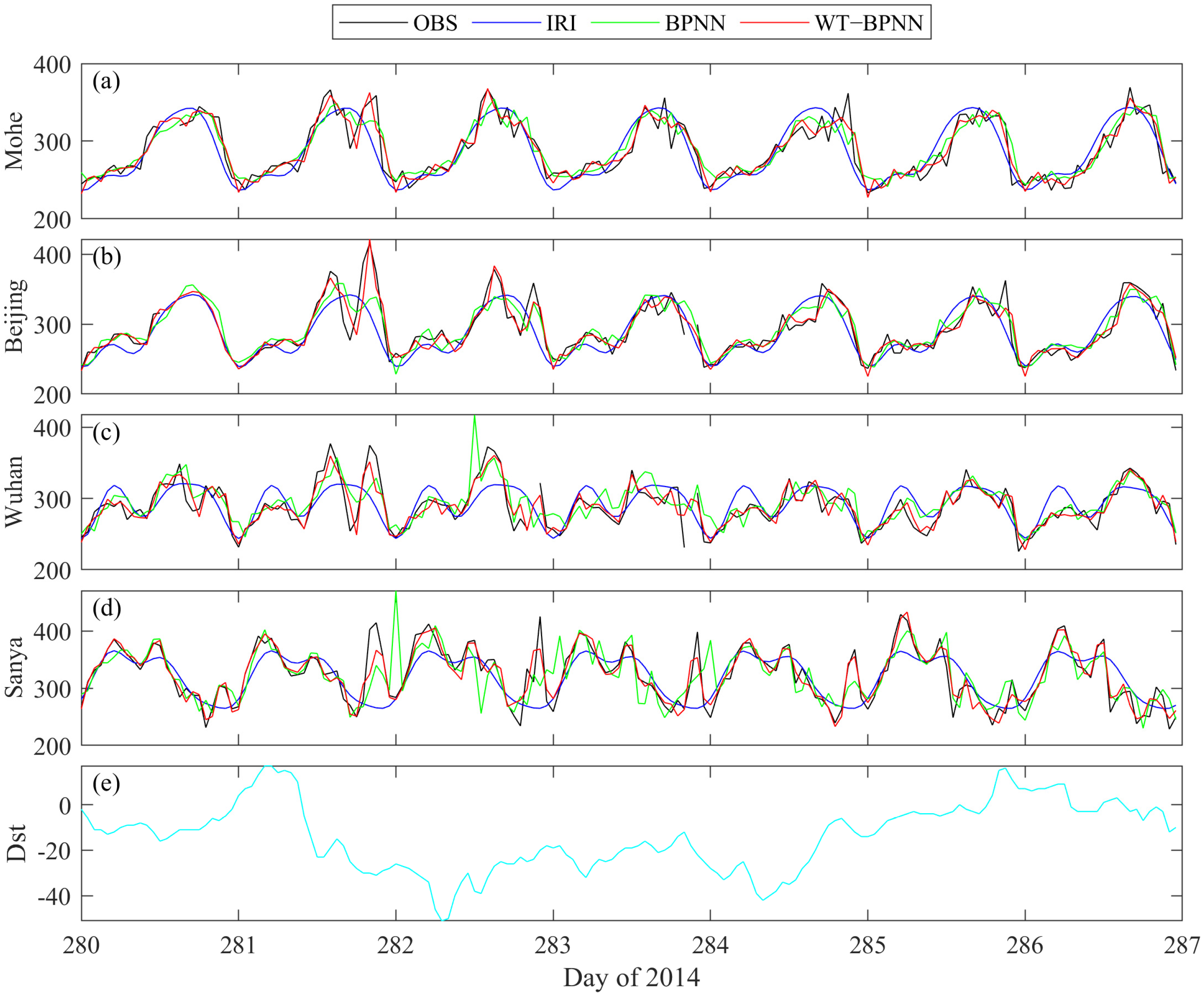
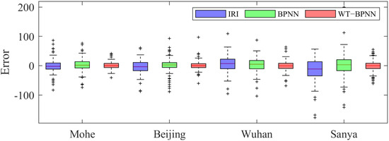
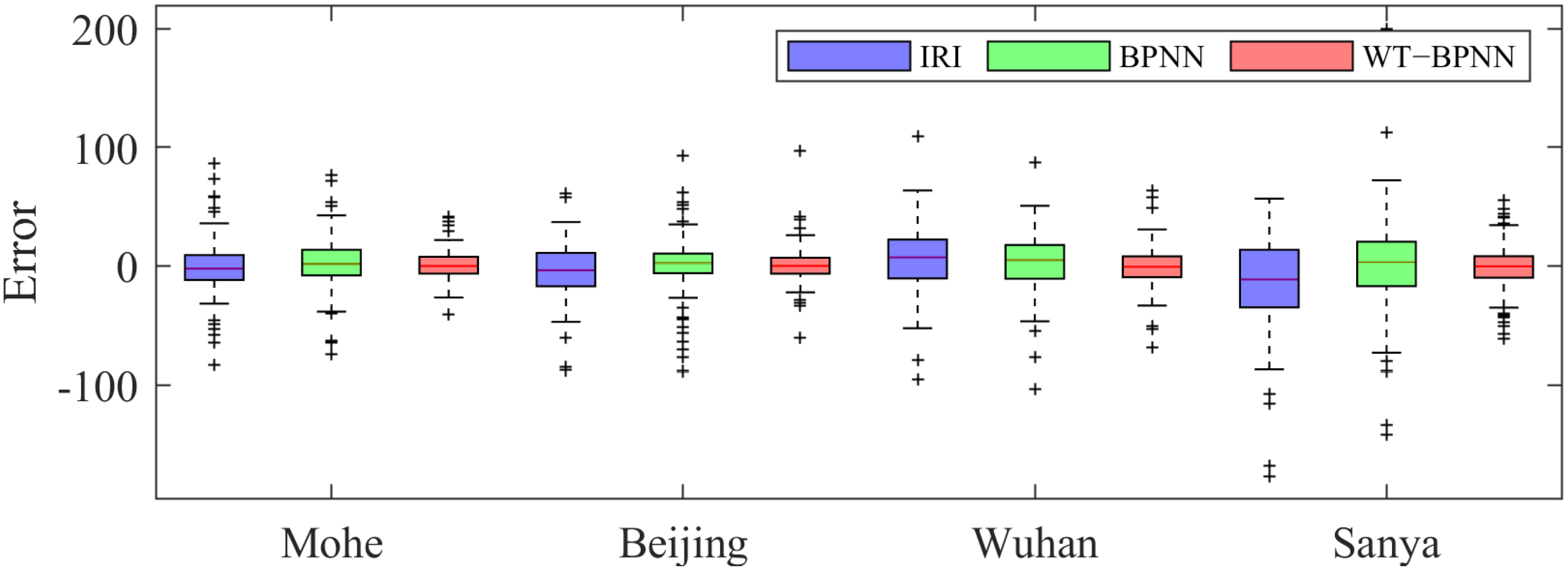
The hmF2 parameter demonstrates distinct diurnal variation influenced by solar activity. To evaluate each model’s forecasting ability, we randomly selected one week of geomagnetic quiet period data from the test set. Figure 6 displays forecasts from the three models for days 280–286 of 2014 at four stations, while Figure 7 presents box plots of the corresponding forecast errors. The minimum value of the geomagnetic index Dst in Figure 6e is −51, indicating that the week is in a geomagnetic quiet period. The observed hmF2 values (OBS) in Figure 6 reveal pronounced diurnal variation, with greater amplitude at lower latitudes. The IRI model generates relatively smooth forecasts but underperforms compared to observations, especially during periods of rapid hmF2 change. This outcome aligns with expectations, as the IRI is a long-term climatological model with limited short-term forecasting capability. The BPNN model captures the general trend in variation more effectively than the IRI model, though notable deviations persist at several time points. In contrast, the model proposed in this study achieves the best overall performance, closely tracking the temporal evolution of hmF2 and accurately forecasting sharp transitions. Additionally, the box plots in Figure 7 show that the WT-BPNN model has the most concentrated forecast error distribution and fewer outliers, indicating superior forecasting reliability. Across stations, all models perform best at the Mohe and Beijing locations, while forecasting accuracy declines with decreasing latitude. Nevertheless, the proposed model consistently demonstrates the highest stability and accuracy among the three models.

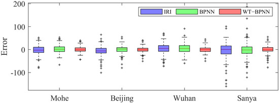
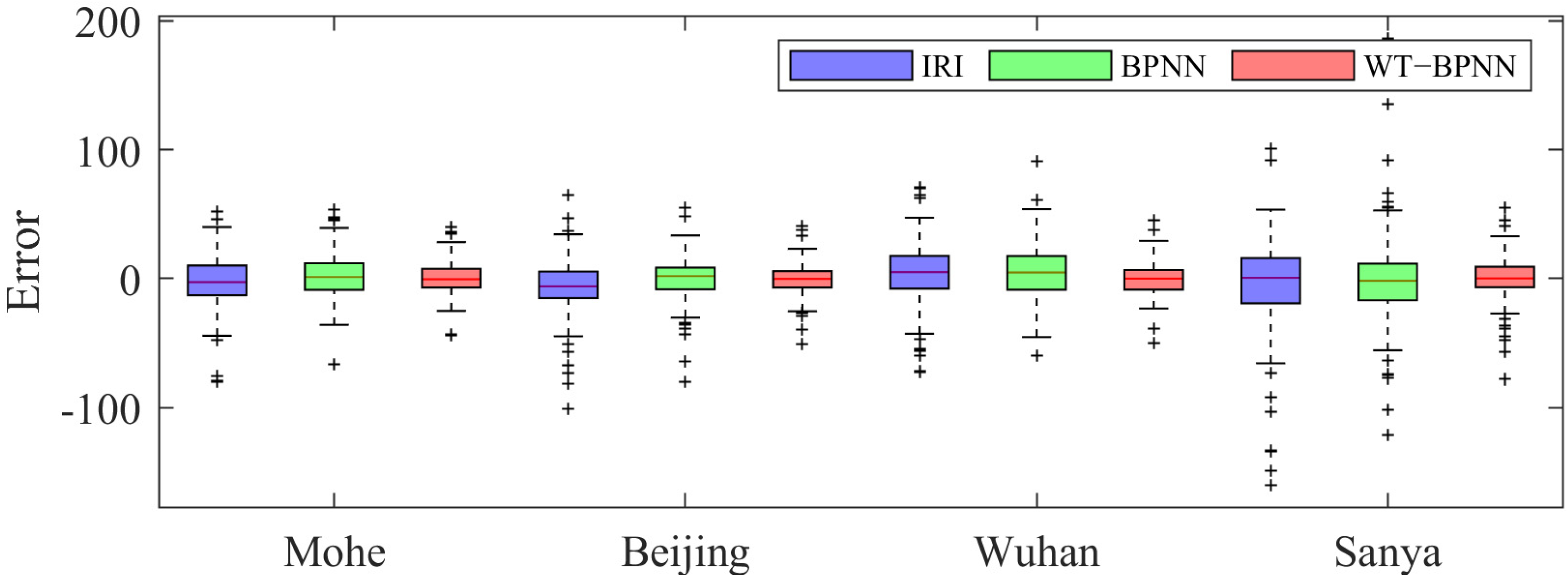
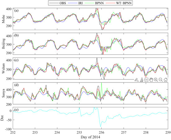
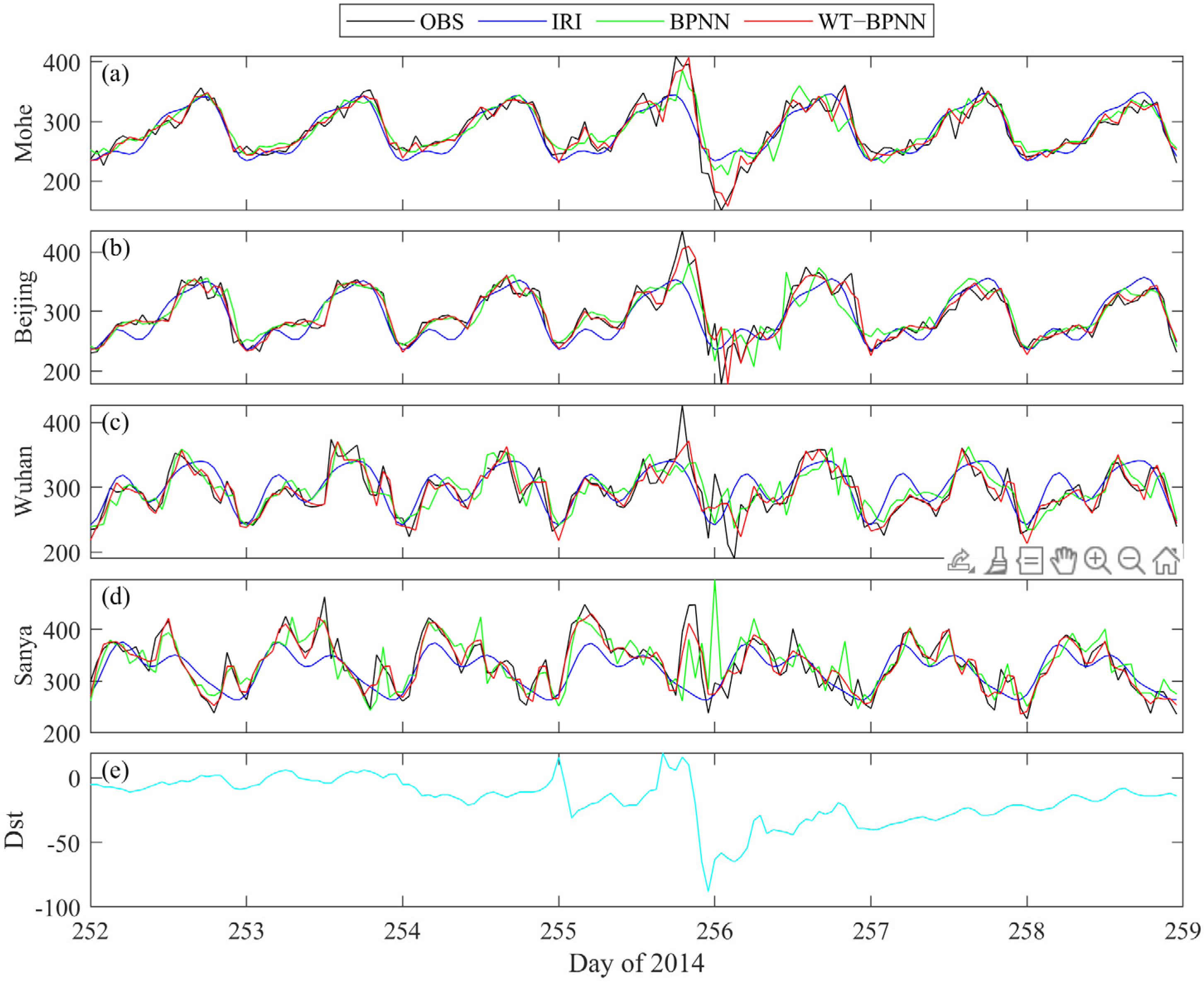
Figure 8e shows that the lowest Dst value on the 255th day of 2014 is −88 at 23:00 UT, and 16 at 19:00 UT. Over a 4 h period, more than 100 changes indicated the occurrence of a severe geomagnetic storm. Data before and after this event are analyzed. Figure 8 presents the forecast results of three models from each station for days 252–258 of 2014, while Figure 9 illustrates the box plots of the corresponding forecast errors. Prior to the geomagnetic storm, all models effectively predicted hmF2 trends, with WT-BPNN achieving the best performance and IRI the worst. During the geomagnetic storm on the 255th day, due to changes in the ionosphere, the OBS data of hmF2 also experienced rapid changes. With the exception of Wuhan station, the WT-BPNN model closely tracked the measured data, demonstrating robust performance. In the recovery phase, all models predicted changes in hmF2, with WT-BPNN again achieving the best results. The error box plots in Figure 9 indicate that WT-BPNN had the most concentrated errors and the fewest outliers, confirming its superior prediction accuracy.

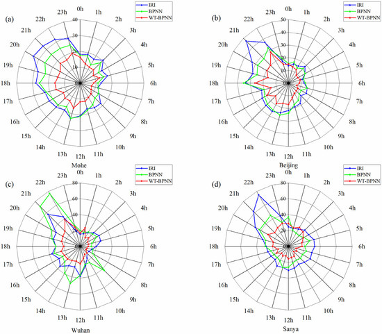
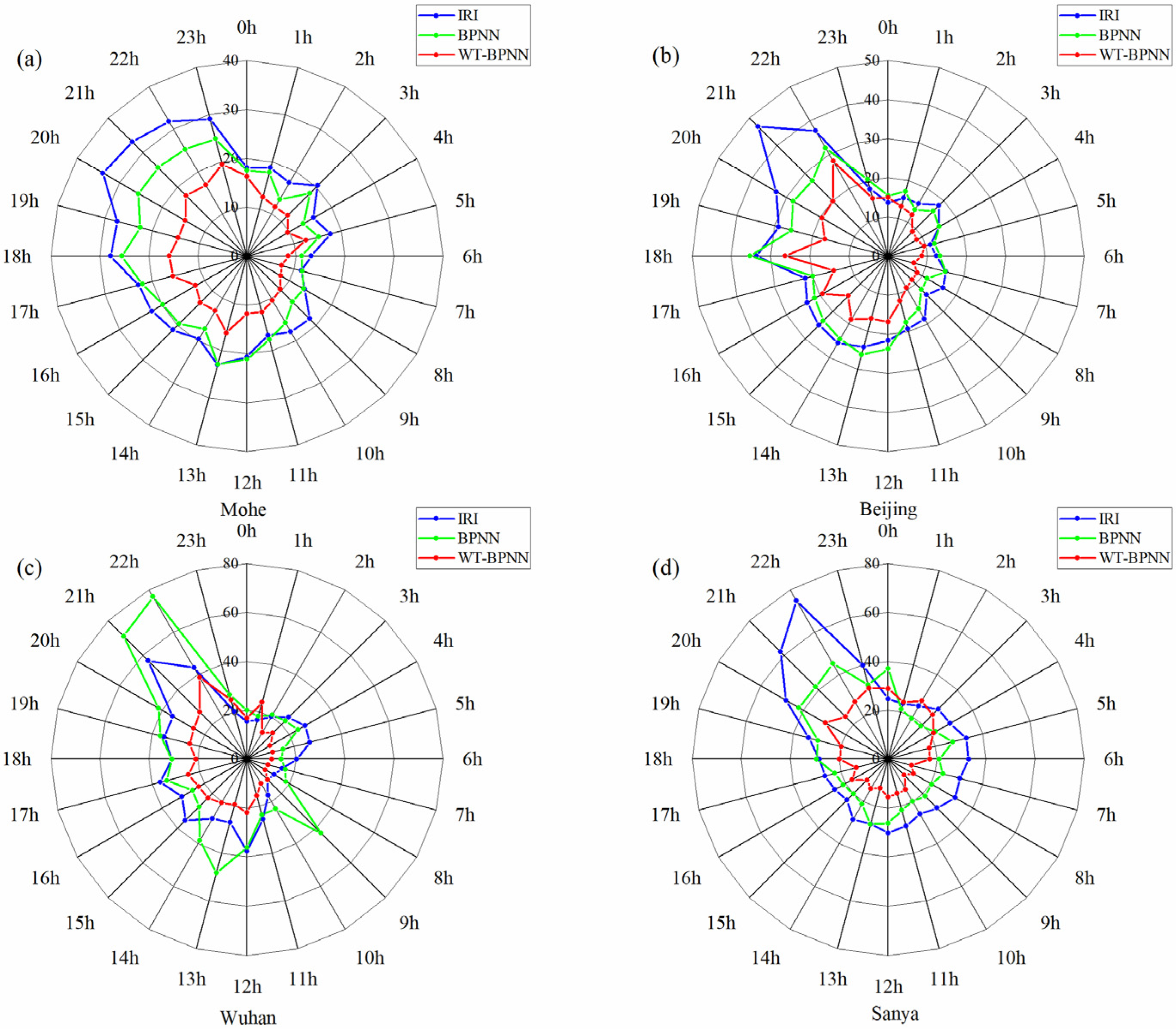
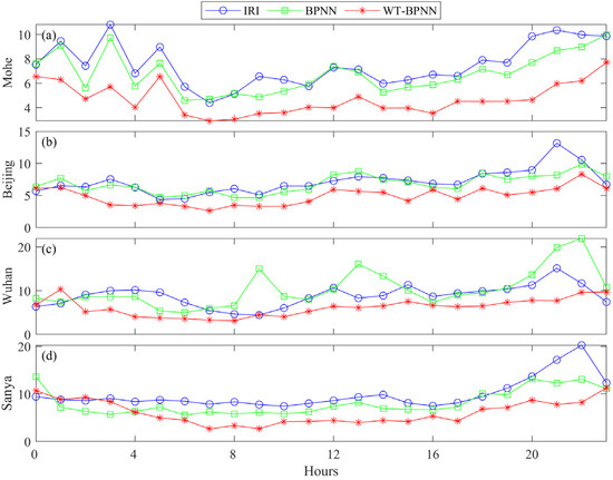
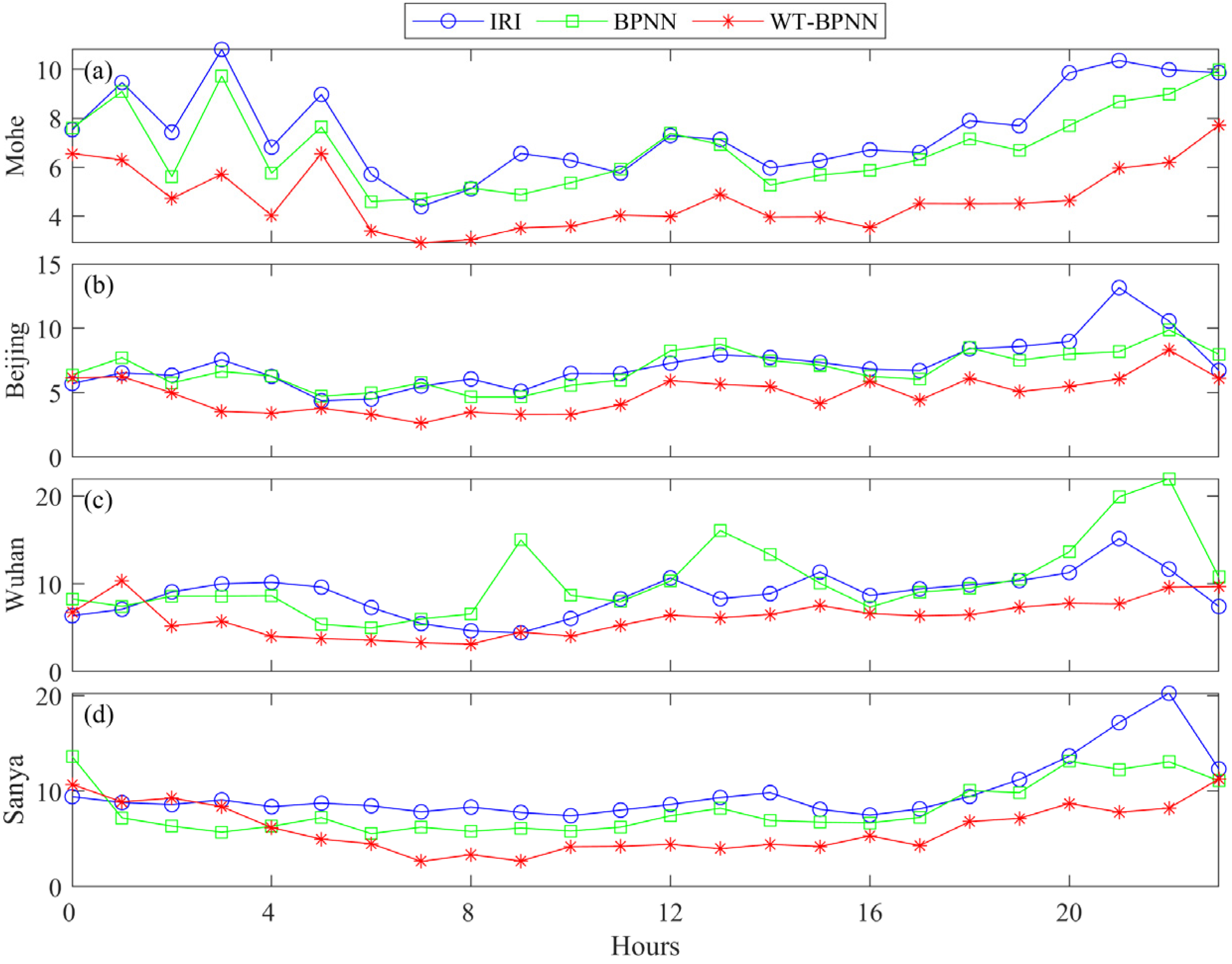
The preceding analysis demonstrates that the ionospheric hmF2 parameter displays a distinct 24 h diurnal variation. To further assess model performance at different times of day, a statistical analysis of the 24 h forecast results was performed across the entire test set. Figure 10 and Figure 11 display the RMSE and RRMSE metrics for each model throughout the 24 h period. All three models can forecast hmF2 over a full day. The WT-BPNN model achieves the highest forecasting accuracy, with RMSE values not exceeding 20 km, 30 km, 40 km, and 40 km at the four stations, respectively. The BPNN model ranks second in performance, while the IRI model demonstrates the lowest accuracy. With the exception of the Wuhan station, the IRI model shows the largest forecast error fluctuations, whereas the WT-BPNN model demonstrates the most stable performance. All three models exhibit relatively large forecast errors between 20:00 and 22:00 UT, accompanied by substantial fluctuations, with the effect most pronounced in the IRI model. In terms of local time (LT = UT + 8), this interval corresponds to the sunrise period, during which the enhanced sunrise effect [26,27] causes rapid changes in ionospheric electron density, resulting in larger hmF2 forecast errors. Conversely, during the local daytime (06:00–10:00 UT), all models exhibit smaller forecast errors and reduced variability. These findings indicate that forecasting performance is generally superior during the daytime than during the nighttime. Overall, the WT-BPNN model is less influenced by the 24 h ionospheric variation and demonstrates more stable forecasting performance than the IRI and BPNN models.

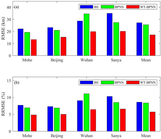
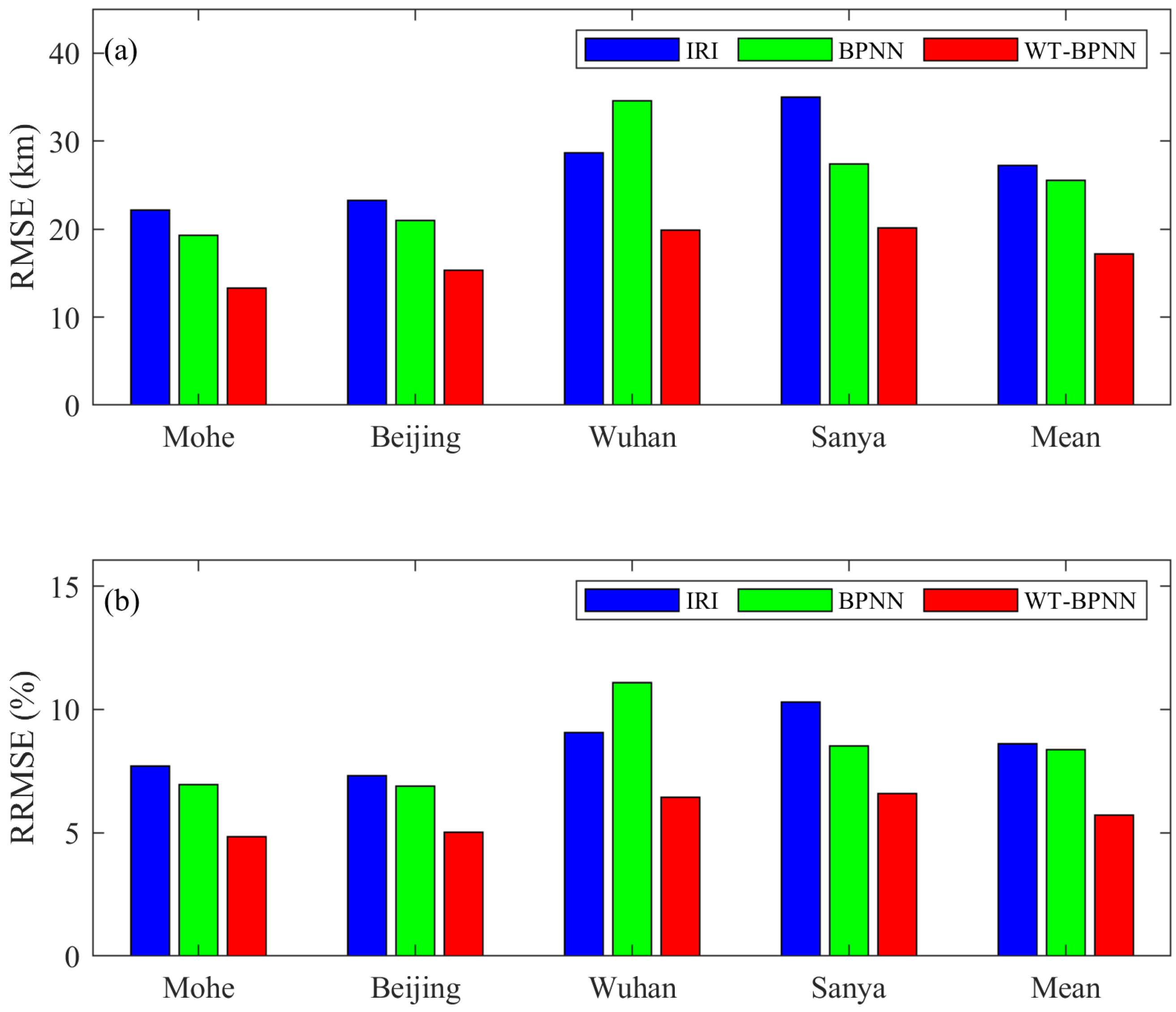
The forecasting performance of the models for 2014 was evaluated by analyzing forecast accuracy at each station using the complete test set and corresponding forecast results.

Table 3. Models’ forecast performance in four stations.

Metrics	IRI		BPNN		WT-BPNN
	RMSE (km)	RRMSE (%)	RMSE (km)	RRMSE (%)	RMSE (km)	RRMSE (%)
Mohe	22.14	7.70	19.29	6.95	13.28	4.85
Beijing	23.23	7.32	20.95	6.91	15.34	5.03
Wuhan	28.67	9.07	34.56	11.07	19.90	6.43
Sanya	35.01	10.31	27.39	8.52	20.13	6.58
Mean	27.26	8.60	25.55	8.36	17.16	5.72

presents the forecast error statistics for the three models at the four stations, while Figure 12 visually compares their performance. According to Table 3 and Figure 12, the IRI model consistently demonstrates the lowest forecasting accuracy, whereas the WT-BPNN model achieves the highest performance across all stations. Regarding average RMSE, the WT-BPNN model attains a value of 17.16 km, which is lower than 10.10 km for the IRI model and 8.39 km for the BPNN model. For RRMSE, the WT-BPNN model achieves 5.72%, which is 2.88% lower than the IRI model and 2.64% lower than the BPNN model. Among the four stations, both the WT-BPNN and IRI models achieve their highest accuracy at the Mohe station and their lowest at the Sanya station, while the BPNN model performs the worst at the Wuhan station. The forecast performance of three models across the four stations exhibits a downward trend with decreasing latitude. This trend is likely attributable to increased solar activity and the pronounced influence of geomagnetic activity in low-latitude regions, which complicates hmF2 forecasting in these areas. The WT-BPNN model exhibits relatively small variations in forecasting accuracy across the four stations, indicating that it is less affected by geographical differences and maintains high forecast capability across high-, mid-, and low-latitude regions. This demonstrates strong suitability for application throughout China. In summary, the improved WT-BPNN model substantially enhances the forecasting accuracy of the hmF2 time series.

5. Conclusions

To address the nonlinear and nonstationary characteristics of the ionospheric hmF2 time series, this study proposes a hybrid short-term forecasting model that integrates the WT with a BPNN. The WT algorithm is employed to decompose and reconstruct the raw hmF2 time series, effectively eliminating noise and outliers while preserving essential feature information. This pre-processed data enables the BPNN to fully utilize its nonlinear mapping capabilities, resulting in more accurate forecasts. Experimental validation using data from four stations in China during 2014 demonstrates that the proposed WT-BPNN model significantly outperforms both the standard BPNN and the empirical IRI models across multiple time scales. In the analysis of diurnal variations, the WT-BPNN model shows strong correspondence with the observed data and greater stability than the benchmark models. Across the entire test set, the WT-BPNN achieves an RMSE of 17.16 km and an average relative RRMSE of 5.72%, indicating substantial improvement in forecasting accuracy over the standalone BPNN model.

In the future, we will incorporate additional input parameters, such as geomagnetic and solar activity indicators, to continuously improve the proposed model, evaluate its forecasting and computational performance for ionospheric foF2, and expand it from a local model in China to a global model.

References

- Zhou, W.; Yu, Y.; Wan, W.; Liu, L. Tidal variations of the ionospheric foF2 in mid-latitude ionosphere. Chin. J. Geophys. 2018, 61, 30–42. (In Chinese) [Google Scholar]
- Wang, J.; Bai, H.; Huang, X.; Cao, Y.; Chen, Q.; Ma, J. Simplified Regional Prediction Model of Long-Term Trend for Critical Frequency of Ionospheric F2 Region over East Asia. Appl. Sci. 2019, 9, 3219. [Google Scholar] [CrossRef] [Scilit]
- Hu, A.; Zhang, K. Using Bidirectional Long Short-Term Memory Method for the Height of F2 Peak Forecasting from Ionosonde Measurements in the Australian Region. Remote Sens. 2018, 10, 1658. [Google Scholar] [CrossRef] [Scilit]
- Bilitza, D.; Pezzopane, M.; Truhlik, V.; Altadill, D.; Reinisch, B.W.; Pignalberi, A. The International Reference Ionosphere Model: A Review and Description of an Ionospheric Benchmark. Rev. Geophys. 2022, 60, e2022RG000792. [Google Scholar] [CrossRef] [Scilit]
- Blanch, E.; Altadill, D. Midlatitude F region peak height changes in response to interplanetary magnetic field conditions and modeling results. J. Geophys. Res. Space Phys. 2012, 117, A12311. [Google Scholar]
- Lin, J.; Yue, X.; Zeng, Z.; Lou, Y.; Shen, X.; Wu, Y.; Schreiner, W.S.; Kuo, Y.-H. Empirical orthogonal function analysis and modeling of the ionospheric peak height during the years 2002–2011. J. Geophys. Res. Space Phys. 2014, 119, 3915–3929. [Google Scholar] [CrossRef] [Scilit]
- Sai Gowtam, V.; Tulasi Ram, S. An Artificial Neural Network-Based Ionospheric Model to Predict NmF2 and hmF2 Using Long-Term Data Set of FORMOSAT-3/COSMIC Radio Occultation Observations: Preliminary Results. J. Geophys. Res. Space Phys. 2017, 122, 11743–11755. [Google Scholar]
- Wang, J.; Yu, Q.; Shi, Y.; Yang, C. A Prediction Method of Ionospheric hmF2 Based on Machine Learning. Remote Sens. 2023, 15, 3154. [Google Scholar]
- Rawer, K.; Lincoln, J.V.; Conkright, R.O. International Reference Ionosphere—IRI 79. In Report UAG-82; World Data Center A for Solar-Terrestrial Physics: Boulder, CO, USA, 1981. [Google Scholar]
- Wang, J.; Yu, Q.; Shi, Y. Comparison of observed hmF2 and the IRI-2020 model for six stations in East Asia during the declining phase of the solar cycle 24. Adv. Space Res. 2024, 73, 2418–2432. [Google Scholar]
- Khuangsatung, S.; Wichaipanich, N.; Nishioka, M. Comparison of ionospheric F2-layer peak height (hmF2) derived by ionosonde with IRI-2020 model over Southeast Asia. Adv. Space Res. 2025, 75, 4175–4191. [Google Scholar]
- Gulyaeva, T.L. Empirical model of ionospheric storm effects on theF2layer peak height associated with changes of peak electron density. J. Geophys. Res. Space Phys. 2012, 117, A02302. [Google Scholar]
- Huang, F.; Ruan, H.; Lei, J.; Zhong, J.; Yue, X.; Li, G.; Chen, Y.; He, J.; Li, N.; Luan, X.; et al. Empirical Models of foF2 and hmF2 Reconstituted by Global Ionosonde and Reanalysis Data and COSMIC Observations. Space Weather 2024, 22, e2023SW003848. [Google Scholar] [CrossRef] [Scilit]
- Wang, J.; Yu, Q.; Shi, Y.; Yang, C.; Ji, S.; Zheng, Y. A New Determining Method for Ionospheric F2-Region Peak Electron Density Height. Remote Sens. 2024, 16, 531. [Google Scholar] [CrossRef] [Scilit]
- Li, W.; Zhao, D.; He, C.; Hu, A.; Zhang, K. Advanced Machine Learning Optimized by The Genetic Algorithm in Ionospheric Models Using Long-Term Multi-Instrument Observations. Remote Sens. 2020, 12, 866. [Google Scholar]
- Iban, M.C.; Şentürk, E. Machine learning regression models for prediction of multiple ionospheric parameters. Adv. Space Res. 2022, 69, 1319–1334. [Google Scholar] [CrossRef] [Scilit]
- Shi, Y.; Yang, C.; Wang, J.; Zheng, Y.; Meng, F.; Chernogor, L.F. A Hybrid Deep Learning-Based Forecasting Model for the Peak Height of Ionospheric F2 Layer. Space Weather 2023, 21, e2023SW003581. [Google Scholar] [CrossRef] [Scilit]
- Rao, T.V.; Sridhar, M.; Ratnam, D.V.; Harsha, P.B.S.; Srivani, I. A Bidirectional Long Short-Term Memory-Based Ionospheric foF2 and hmF2 Models for a Single Station in the Low Latitude Region. IEEE Geosci. Remote Sens. Lett. 2021, 19, 8005405. [Google Scholar] [CrossRef] [Scilit]
- Zhang, B.; Wang, Z.; Shen, Y.; Li, W.; Xu, F.; Li, X. Evaluation of foF2 and hmF2 Parameters of IRI-2016 Model in Different Latitudes over China under High and Low Solar Activity Years. Remote Sens. 2022, 14, 860. [Google Scholar]
- Ghaffari Razin, M.R.; Voosoghi, B. Modeling of ionosphere time series using wavelet neural networks (case study: N-W of Iran). Adv. Space Res. 2016, 58, 74–83. [Google Scholar] [CrossRef] [Scilit]
- Babu, C.N.; Reddy, B.E. A moving-average filter based hybrid ARIMA-ANN model for forecasting time series data. Appl. Soft Comput. 2014, 23, 27–38. [Google Scholar] [CrossRef] [Scilit]
- Hajiabotorabi, Z.; Kazemi, A.; Samavati, F.F.; Maalek Ghaini, F.M. Improving DWT-RNN model via B-spline wavelet multiresolution to forecast a high-frequency time series. Expert Syst. Appl. 2019, 138, 112842. [Google Scholar] [CrossRef] [Scilit]
- Tian, Z.; Li, S.; Wang, Y.; Sha, Y. A prediction method based on wavelet transform and multiple models fusion for chaotic time series. Chaos Solitons Fractals 2017, 98, 158–172. [Google Scholar]
- Wichaipanich, N.; Hozumi, K.; Supnithi, P.; Tsugawa, T. A comparison of neural network-based predictions of foF2 with the IRI-2012 model at conjugate points in Southeast Asia. Adv. Space Res. 2017, 59, 2934–2950. [Google Scholar] [CrossRef] [Scilit]
- Habarulema, J.B.; McKinnell, L.A. Investigating the performance of neural network backpropagation algorithms for TEC estimations using South African GPS data. Ann. Geophys. 2012, 30, 857–866. [Google Scholar] [CrossRef] [Scilit]
- Shi, Y.; Yang, C.; Wang, J.; Zhang, Z.; Meng, F.; Bai, H. A Forecasting Model of Ionospheric foF2 Using the LSTM Network Based on ICEEMDAN Decomposition. IEEE Trans. Geosci. Remote Sens. 2023, 61, 4108416. [Google Scholar] [CrossRef] [Scilit]
- Chen, J.; Wang, W.; Lei, J.; Dang, T. The Physical Mechanisms for the Sunrise Enhancement of Equatorial Ionospheric Upward Vertical Drifts. J. Geophys. Res. Space Phys. 2020, 125, e2020JA028161. [Google Scholar] [CrossRef] [Scilit]
Disclaimer/Publisher’s Note: The statements, opinions and data contained in all publications are solely those of the individual author(s) and contributor(s) and not of MDPI and/or the editor(s). MDPI and/or the editor(s) disclaim responsibility for any injury to people or property resulting from any ideas, methods, instructions or products referred to in the content. |
© 2026 by the authors. Licensee MDPI, Basel, Switzerland. This article is an open access article distributed under the terms and conditions of the Creative Commons Attribution (CC BY) license.