Air Pollution in 88 US Metropolitan Areas: Trends and Persistence

Abstract

This paper analyses trends and persistence in air pollution levels in 88 US metropolitan areas using fractional integration methods. The results indicate that the differencing parameter d is higher than 0 in 38 of the series, which supports the hypothesis of long-memory behavior and implies that, although the effects of shocks are long-lived, they eventually die out. The highest degrees of persistence are found in the Fresno, Bakersfield, Bradenton and San Diego areas. On the whole, the gathered evidence indicates that regional differences in pollution levels are significant, with factors such as industrialisation history and extreme weather events playing a crucial role in their degree of persistence. This suggests that, in order to tackle pollution more effectively, federal environmental policies, such as the Clean Air Act, should be complemented by more targeted ones taking into account local characteristics.

1. Introduction

Environmental pollution is one of the most pressing challenges faced by mankind owing to its severe consequences for human health, ecosystems and sustainable development. It has become a major concern in the US, especially in the case of the most populated urban areas. The Environmental Protection Agency (EPA) estimates that, in 2022, about 60% of the US population was exposed to hazardous levels of pollution in some form [1]. In response to this threat the US government introduced the Clean Air Act which sets national standards for air quality and has provided a framework for reducing pollutants such as sulphur dioxide and particulate matter [2].

Understanding how pollution levels have evolved over time is crucial to evaluate the effectiveness of environmental policies and to develop future strategies to respond to the increasing challenges posed by climate change. For this purpose, the present study examines pollution trends in 88 US metropolitan areas over the period 1980–2023 using fractional integration techniques. This statistical approach is most suitable for time series with long-memory properties and persistent dynamics that cannot be adequately modelled using traditional methods. In particular, the main advantage of the fractional integration approach [3] is that it allows the differencing parameter d to be any real number, including fractional ones, and thus captures more accurately both long- and short-term correlations [4]. Moreover, it yields efficient estimates and more robust results [5,6].

The analysis in this paper provides new, comprehensive evidence on the stochastic properties of pollution in the 88 US metropolitan areas considered, specifically on the possible presence of trends and on the degree of persistence of the series under investigation. Such information is essential to design more targeted and effective policies to reduce pollution and mitigate its adverse effects.

The layout of the paper is the following: Section 2 briefly reviews the relevant literature; Section 3 describes the data; Section 4 outlines the econometric framework based on the concept of fractional integration; Section 5 presents the empirical results; Section 6 offers some concluding remarks.

2. Literature Review

There exists an extensive literature on air pollution in the US and its adverse effects on public health, numerous papers identifying various diseases and chronic conditions that are strongly associated with continued exposure to high levels of air pollutants. These studies have addressed both the immediate consequences and long-term effects of exposure to air pollutants, paying particular attention to vulnerable groups such as children, the elderly, and low-income communities. In particular, several studies analyse the impacts on children, highlighting effects on cognitive development and executive function [7]. Other studies focus on older adults and patients with chronic diseases, who are more susceptible to pollution and extreme weather events [8]. There is also abundant evidence that low-income and socially disadvantaged communities are disproportionately affected by air pollution due to factors such as residential segregation and proximity to emission sources [9,10,11]. Finally, other studies analyse the general effects of air pollution on the health of the population as a whole, with particularly relevant implications for these vulnerable groups [12,13,14,15], among others. In addition to health effects, the economic costs of air pollution in the US have also been analysed in depth—these include direct and indirect expenses related to medical care, loss of labour productivity, and the impact on sectors such as agriculture and tourism [16,17,18,19]. This evidence shows not only the magnitude of the environmental problem, but also its social and economic impact.

Environmental inequality in the US is another central theme in pollution studies. Low-income communities, particularly those located in highly industrialised urban areas, are disproportionately affected by air pollution, which contributes to greater inequality in terms of health, access to quality services, and living conditions [11,20]. Studies on this topic highlight the urgent need for reducing social and environmental disparities through inclusive policies and a comprehensive approach to improving the quality of life of all citizens.

The cumulative effects of historical factors, seasonal variations, and regulatory interventions have resulted in highly complex patterns of behaviour in US pollution levels. This country is responsible for approximately 25% of historical global CO₂ emissions [21]. In fact, US greenhouse gas emissions account for 79.7% of global ones [1], which implies that the US has a key role in mitigating the effects of climate change by implementing effective policies to reduce pollutant emissions and improve air quality. Climate change and pollution are problems that cannot be addressed in isolation; an integrated approach is needed to achieve a healthier and more sustainable future.

The present study contributes to a specific branch of the literature modelling atmospheric pollution series by means of fractional integration techniques. This approach, relatively new in environmental analysis, is ideal for analysing time series, such as air pollutant concentrations, with long-memory properties and persistent patterns driven by a range of historical and seasonal factors. The usefulness of this framework for modelling pollution series with long-term dependence has been shown in various recent studies [22,23,24,25,26], among others; the long memory detected in many pollution time series indicates that present pollution levels have a significant influence on future ones, which makes monitoring and early intervention to mitigate their effects extremely important.

However, other studies using this approach find that pollution may be absorbed by natural systems and that changes in environmental policies or interventions may affect its long-run trends. For instance, Caporale et al. [25] reported mean reversion in PM₁₀ concentrations in eight European capitals from 2014 to 2020, which implies that the effects of environmental shocks on those series are not permanent, but tend to be corrected over time. Similarly, Bermejo et al. [26] concluded that mean reversion occurs in PM_2.5 concentrations in 20 global megacities between 2018 and 2020, and thus that shocks have transient effects.

In another study, Gil-Alana et al. [27] examined global and per capita Nitrogen Oxides (NO_x) and volatile organic compounds (VOC) emissions in the US from 1914 to 2014 and also the effectiveness of environmental policies; they found that by 2014 the US had managed to reduce both VOC and NO_x per capita emission levels compared to 1970. In two additional studies, Gil-Alana et al. [28] investigated the time evolution of CO₂ emissions in the European Union, while Gil-Alana et al. [23] examined air quality in the 50 US states, focusing on PM₁₀ and PM_2.5 pollutants, and concluded that shocks and policy actions have long-lived effects at both the local and national levels. Finally, other research has focused on the convergence of pollutant series in US regions [29,30]. All these studies indicate that long memory and persistence are two important properties of pollutants in the US.

3. Data Description

The series used for the analysis provide information about air quality in 88 US metropolitan areas by measuring the number of days between 1980 and 2023 when the Air Quality Index (AQI) exceeded a threshold of 100. Such a value indicates poor air quality (i.e., within the unhealthy range), and that on the day in question at least one of the pollutants exceeded the level consistent with the set air quality standards [31].

The Air Quality Index (AQI) used in this study is defined in accordance with the official methodology of the United States Environmental Protection Agency (EPA). Within this framework, an AQI value of 100 corresponds to the upper limit of the Moderate category and defines the threshold above which air quality is classified as Unhealthy for Sensitive Groups. According to the EPA’s conversion functions, this value is associated with concentrations of 35.4 µg/m³ for PM₂.₅ (24 h moving average), 154 µg/m³ for PM₁₀ (24 h), 70 ppb for ozone (8 h average), 100 ppb for NO₂ (1 h), 75 ppb for SO₂ (1 h), and 9.4 ppm for CO (8 h average). The daily AQI is defined as the maximum of the sub-indices corresponding to these pollutants; consequently, days with an AQI greater than 100 indicate that at least one of them has exceeded the regulatory threshold defined by the EPA [31]. Note that historical AQI data are at times revised. The main reason is that changes to the National Ambient Air Quality Standards (NAAQS) are applied retroactively to data from previous years to provide consistent comparisons over time. This information is compiled by the Environmental Protection Agency (EPA) and is updated regularly as air quality standards change.

The data have been retrieved from the database of the Bureau of Transportation Statistics, United States Department of Transportation, available at: https://www.bts.gov/content/air-pollution-trends-selected-metropolitan-statistical-areas (accessed on 11 December 2024). The data source is: U.S. Environmental Protection Agency, Office of Air and Radiation, Air Trends, Air Quality Index: Daily AQI, available at https://aqs.epa.gov/aqsweb/airdata/download_files.html (accessed on 11 December 2024).

Table 1. Descriptive Statistics.

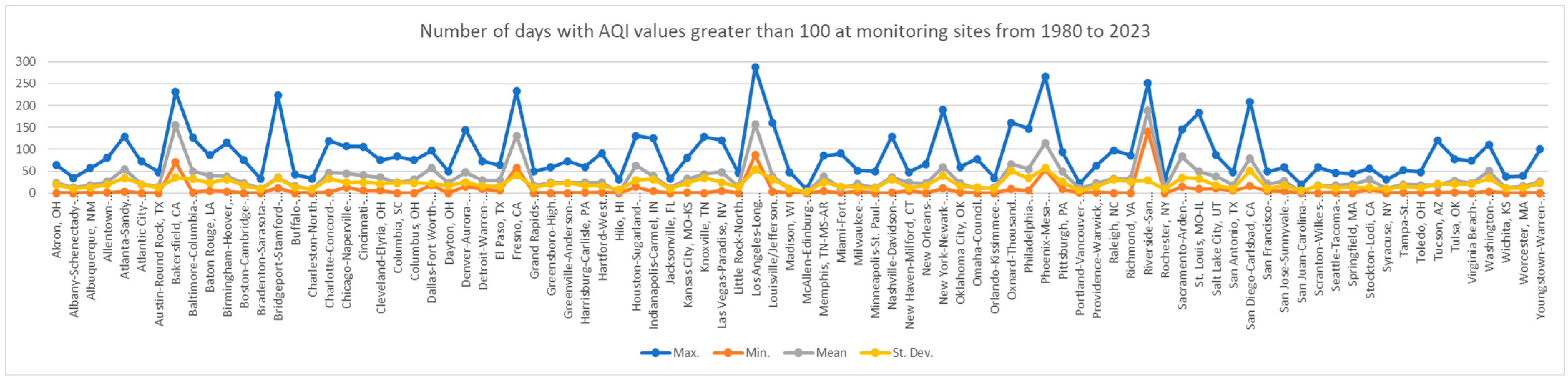
District	Acronym	Max.	Min.	Mean	St. Dev.
Akron, OH	AKRON	65	0	22.97	19.18
Albany-Schenectady-Troy, NY	ALBAN	35	0	12.19	9.98
Albuquerque, NM	ALBUQ	57	1	18.31	13.04
Allentown-Bethlehem-Easton, PA	ALLEN	80	1	25.50	19.04
Atlanta-Sandy Springs-Roswell, GA	ATLAA	129	3	54.94	35.08
Atlantic City-Hammonton, NJ	ATLIC	72	0	19.50	20.09
Austin-Round Rock, TX	AUSTI	48	0	15.25	12.20
Bakersfield, CA	BAKER	231	70	154.86	35.52
Baltimore-Columbia-Towson, MD	BALTM	127	2	49.83	32.04
Baton Rouge, LA	BATON	87	5	39.53	23.56
Birmingham-Hoover, AL	BIRMG	115	3	38.44	31.36
Boston-Cambridge-Newton, MA-NH	BOSTN	75	0	22.08	17.15
Bradenton-Sarasota-Venice, FL	BRADE	32	0	10.08	9.49
Bridgeport-Stamford-Norwalk, CT	BRIDG	223	12	35.83	33.91
Buffalo-Cheektowaga-Niagara Falls, NY	BUFFL	42	0	16.03	13.30
Charleston-North Charleston, SC	CHLTN	33	0	8.67	8.96
Charlotte-Concord-Gastonia, NC-SC	CHRLT	119	2	46.67	33.29
Chicago-Naperville-Joliet, IL-IN-WI	CHICG	107	13	45.00	24.20
Cincinnati-Middletown, OH-KY-IN	CINCN	106	6	40.19	25.25
Cleveland-Elyria, OH	CLEVL	75	6	35.31	21.30
Columbia, SC	CLMBA	84	0	23.78	23.21
Columbus, OH	COLUM	75	0	30.75	23.09
Dallas-Fort Worth-Arlington, TX	DALLA	97	18	56.94	21.21
Dayton, OH	DAYTN	50	0	23.08	16.24
Denver-Aurora-Lakewood, CO	DENVR	144	15	47.08	24.86
Detroit-Warren-Dearborn, MI	DETRT	73	9	29.03	15.52
El Paso, TX	ELPAS	64	6	28.86	14.93
Fresno, CA	FRESN	233	58	130.61	41.01
Grand Rapids-Wyoming, MI	GRAND	50	0	17.31	13.41
Greensboro-High Point, NC	GRNBO	59	0	23.81	20.89
Greenville-Anderson-Mauldin, SC	GRNVL	73	0	23.56	23.32
Harrisburg-Carlisle, PA	HARRB	60	1	24.19	17.47
Hartford-West Hartford-East Hartford, CT	HARTW	91	2	24.42	16.45
Hilo, HI	HILO	31	0	2.58	7.07
Houston-Sugarland-Baytown, TX	HOUST	131	14	63.08	29.64
Indianapolis-Carmel, IN	INDIA	125	4	38.75	31.32
Jacksonville, FL	JAKVL	32	0	11.69	9.66
Kansas City, MO-KS	KANSC	81	1	32.19	22.95
Knoxville, TN	KNOXV	128	0	43.19	34.61
Las Vegas-Paradise, NV	LVEGS	121	5	48.28	24.67
Little Rock-North Little Rock-Conway, AR	LTTRK	46	0	16.00	14.33
Los Angeles-Long Beach-Anaheim, CA	LANGL	287	87	157.14	54.14
Louisville/Jefferson County, KY-IN	LOUVL	161	3	38.47	31.77
Madison, WI	MADIS	48	0	9.61	9.73
McAllen-Edinburg-Mission, TX	MCALL	9	0	2.08	2.73
Memphis, TN-MS-AR	MEMPS	85	4	37.14	25.19
Miami-Fort Lauderdale-West Palm Beach, FL	MIAMI	90	1	11.83	15.22
Milwaukee-Waukesha-West Allis, WI	MILWK	51	3	20.75	13.37
Minneapolis-St. Paul-Bloomington, MN-WI	MINNP	50	0	12.64	11.04
Nashville-Davidson-Murfreesboro-Franklin, TN	NASHV	129	1	36.14	31.11
New Haven-Milford, CT	NHAVN	48	5	23.67	11.64
New Orleans-Metairie, LA	NORLS	66	0	22.22	16.53
New York-Newark-Jersey City, NY-NJ-PA	NYORK	190	11	60.00	39.55
Oklahoma City, OK	OKLAH	60	2	22.53	15.50
Omaha-Council Bluffs, NE-IA	OMAHA	78	0	10.36	13.54
Orlando-Kissimmee-Sanford, FL	ORLND	35	0	12.17	9.78
Oxnard-Thousand Oaks-Ventura, CA	OXNRD	161	9	66.31	50.18
Philadelphia-Camden-Wilmington, PA-NJ-DE-MD	PHILD	147	6	54.83	33.71
Phoenix-Mesa-Scottsdale, AZ	PHOEN	267	54	114.22	57.22
Pittsburgh, PA	PITTS	94	9	48.75	25.93
Portland-Vancouver-Hillsboro, OR-WA	PORTL	22	1	10.75	6.04
Providence-Warwick, RI-MA	PROVD	63	2	22.25	14.86
Raleigh, NC	RALGH	98	0	32.97	30.73
Richmond, VA	RICHM	86	0	32.19	26.15
Riverside-San Bernardino-Ontario, CA	RIVSD	251	141	188.06	28.83
Rochester, NY	ROCHT	32	0	10.50	9.48
Sacramento-Arden-Arcade-Roseville, CA	SACRM	145	14	83.39	34.44
St. Louis, MO-IL	STLOU	183	9	48.94	33.23
Salt Lake City, UT	SALTL	87	11	37.94	17.51
San Antonio, TX	SANTO	47	6	18.19	10.18
San Diego-Carlsbad, CA	SDIEG	209	16	79.39	51.05
San Francisco-Oakland-Hayward, CA	SFRAN	49	5	20.31	10.32
San Jose-Sunnyvale-Santa Clara, CA	SJOSE	59	4	27.53	17.47
San Juan-Carolina-Caguas, PR	SJUAN	19	0	3.67	5.97
Scranton-Wilkes-Barre-Hazleton, PA	SCRNT	59	0	17.47	16.28
Seattle-Tacoma-Bellevue, WA	SEATL	46	2	17.28	11.23
Springfield, MA	SPRING	44	0	20.06	14.02
Stockton-Lodi, CA	STOCK	56	9	30.94	12.54
Syracuse, NY	SYRAC	31	0	10.00	8.98
Tampa-St. Petersburg-Clearwater, FL	TAMPA	52	1	19.67	15.36
Toledo, OH	TOLED	48	1	18.47	12.78
Tucson, AZ	TUCSN	120	1	18.39	20.42
Tulsa, OK	TULSA	78	2	28.25	20.42
Virginia Beach-Norfolk-Newport News, VA-NC	VIRGN	74	0	22.39	20.62
Washington-Arlington-Alexandria, DC-VA-MD-WV	WASHT	111	3	50.19	33.69
Wichita, KS	WICHT	37	0	11.86	10.67
Worcester, MA	WORCT	39	0	15.97	12.13
Youngstown-Warren-Boardman, OH	YOUNG	100	0	26.81	22.11

Note: this table reports the maximum and minimum value, the mean and the standard deviation for each AQI series.

and Figure 1 display some descriptive statistics of the series for the 88 US metropolitan areas considered, such as the maximum and minimum value, the mean and the standard deviation of the number of days exceeding 100 in the AQI between1980 and 2023, that is, days with air quality considered unhealthy or worse. It can be seen that seven of the areas considered have more than 200 days per year in this category, namely: Bakersfield, CA; Bridgeport-Stamford-Norwalk, CT; Fresno, CA; Phoenix-Mesa-Scottsdale, AZ; Riverside-San Bernardino-Ontario, CA; San Diego-Carlsbad, CA. In particular, the highest value is observed in the case of Los Angeles-Long Beach-Anaheim, CA, with a record of 287 days with an AQI > 100 in 1980, i.e., days with air quality considered unhealthy or worse. However, this number has decreased almost every year, reaching 87 days in 2023, which results in a mean value of 157.14 days with a standard deviation of 54.14. By contrast, McAllen-Edinburg-Mission, TX exhibits the lowest number of poor air quality days, with an AQI higher than 100 for 9 days in 2003, and equal to 0 in 16 of the 43 years within the sample period, with a mean value of only 2.07 days and a standard deviation of 2.73.

4. Modelling Framework

Long memory is a widely observed feature in hydrological and climatological data (including air pollution ones, as previously mentioned). In such a case the spectral density function of a stationary process has one or more poles or singularities in the spectrum, which in environmental series often corresponds to the zero frequency. This is normally interpreted as implying that the series should be first-differenced [32,33]; however, the spectrum of the first-differenced data is often close to zero at the zero frequency, which suggests that over-differentiation has occurred. This finding motivates the fractional integration approach, which is suitable for series requiring a degree of differentiation higher than 0 but lower than 1.

To be more precise, an I(d) or fractionally integrated process is defined as:

(1 − L)^d x(t) = u(t)

(1)

where L is the backshift (lag) operator (Lx(t) = x(t − 1)), d can be any real number (including fractional ones), and u(t) is an I(0) process, which in its simplest form can be a white noise one characterized by zero mean, constant variance and uncorrelated terms.

An appealing feature of such a model is its generality, since it encompasses trend stationary models (if d = 0) as in DeJong et al. [34,35], nonstationary unit roots as in Nelson and Plosser [36] (if d = 1), but also additional cases corresponding to fractional values, namely:

(i)

Anti-persistence, if d < 0;

(ii)

Long-memory covariance stationarity, if 0 < d < 0.5;

(iii)

Non-stationarity and mean reversion, if 0.5 ≤ d < 1;

(iv)

Long memory after taking first differences, i.e., I(d) with d > 1.

In the present context, the most relevant case might be (iii), when the series is non-stationary but the effects of shocks are transitory and disappear in the long run.

The polynomial in L in Equation (1) can be expanded as in the following expression:

$${\left(1-L\right)}^d = {\sum }_{j=1}^{\infty }{\displaystyle \frac{\mathsf{\Gamma }\left(\mathrm{d}-1\right) {\left(-L\right)}^j}{\mathsf{\Gamma }\left(\mathrm{d}-\mathrm{j}+1\right)\mathsf{\Gamma }\left(\mathrm{j}+1\right)}} ,$$

(2)

where Γ is the gamma function, which is defined as:

$$\mathsf{\Gamma }\left(\mathrm{z}\right)= {\int }_0^{\infty }{t}^{z-1}{e}^{-t}d\left(t\right).$$

(3)

Positive values of d imply ’long memory’, namely strong dependence between observations far apart in time. The higher the value of d is, the higher will be their degree of dependence, which implies that shocks will have highly persistent effects and the spectral density function will be unbounded at the origin.

For the analysis we use a simple version of the testing procedure developed by Robinson [37] which is valid for testing the null hypothesis: H0: d = d0, for any real value d0 in a fractional model such as the one given by Equation (1). In particular, we use iterations for values of d0 from −2 to 2 with 0.01 increments, reporting the confidence bands of d0-values for which H0 cannot be rejected at the 5% level. This method is based on the Lagrange Multiplier principle and has a standard null and local limit distributions independently of the values of d0, which is a very desirable feature of this test. In addition, the same standard limit behavior holds if one includes deterministic terms such as a constant or a linear time trend. It is also the most efficient method in the Pitman sense against local departures. All these features make this procedure very attractive for empirical applications involving fractional differentiation.

5. Empirical Results

Let x(t) in Equation (1) be the errors in a regression model that includes a constant and a linear time trend, namely:

y(t) = α + β t + x(t), (1 − L)^d x(t) = u(t), t = 1, 2, …

(4)

where y(t) denotes the observed series and u(t) is a white noise process.

Table 2. Estimates of d.

Series	No Deterministic Terms	An Intercept	An Intercept and a Linear Time Trend
AKRON	0.54   (0.39,   0.75)	0.41   (0.31,   0.54)	0.11  (−0.08,   0.36)
ALBAN	0.47   (0.31,   0.72)	0.35   (0.24,   0.51)	0.10  (−0.10,   0.37)
ALBUQ	0.22  (−0.02,   0.49)	0.18  (−0.02,   0.48)	0.17  (−0.07,   0.67)
ALLEN	0.54   (0.34,   0.83)	0.41   (0.29,   0.58)	0.19  (−0.09,   0.71)
ATLAA	0.65   (0.49,   0.89)	0.51   (0.39,   0.71)	0.32   (0.10,   0.65)
ATLIC	0.54   (0.37,   0.79)	0.40   (0.29,   0.52)	0.11  (−0.09,   0.41)
AUSTI	0.40   (0.24,   0.64)	0.30   (0.17,   0.48)	0.01  (−0.19,   0.31)
BAKER	0.81   (0.61,   1.09)	0.76   (0.55,   1.12)	0.75   (0.52,   1.12)
BALTM	0.63   (0.44,   0.91)	0.44   (0.34,   0.56)	−0.08 (−0.35,   0.31)
BATON	0.70   (0.51,   1.00)	0.50   (0.37,   0.70)	0.19  (−0.04,   0.58)
BIRMG	0.74  (0.54,    1.09)	0.68   (0.48,    1.05)	0.65   (0.41,    1.05)
BOSTN	0.50   (0.31,   0.79)	0.38   (0.24,   0.58)	0.19  (−0.11,   0.88)
BRADE	0.76   (0.59,   1.07)	0.73   (0.54,   1.06)	0.72   (0.49,   1.06)
BRIDG	0.07  (−0.21,   0.43)	0.04  (−0.15,   0.30)	0.12  (−0.18,   0.42)
BUFFL	0.46   (0.27,   0.74)	0.35   (0.21,   0.53)	0.16  (−0.04,   0.46)
CHLTN	0.44   (0.24,   0.74)	0.35   (0.19,   0.62)	0.12  (−0.25,   0.78)
CHRLT	0.65   (0.49,   0.89)	0.49   (0.37,   0.69)	0.35   (0.12,   0.74)
CHICG	0.54   (0.37,   0.79)	0.34   (0.19,   0.53)	0.16  (−0.10,   0.50)
CINCN	0.40   (0.24,   0.64)	0.35   (0.22,   0.53)	0.06  (−0.18,   0.45)
CLEVL	0.81   (0.61,   1.09)	0.47   (0.36,   0.61)	0.28   (0.11,   0.51)
CLMBA	0.63   (0.44,   0.91)	0.35   (0.23,   0.52)	0.16  (−0.07,   0.50)
COLUM	0.70   (0.51,   1.00)	0.41   (0.30,   0.55)	0.11  (−0.07,   0.38)
DALLA	0.74   (0.54,    1.09)	0.52  (0.35,    0.87)	0.41  (0.08,    0.87)
DAYTN	0.50   (0.31,   0.79)	0.38   (0.27,   0.73)	0.17  (−0.03,   0.41)
DENVR	−0.09   (−0.21,   0.60)	−0.06  (−0.35,  1.18)	0.12  (−0.15,  1.17)
DETRT	0.42   (0.23,   0.69)	0.29   (0.15,    0.47)	0.11  (−0.12,   0.44)
EL   PAS	0.60   (0.39,   0.90)	0.41   (0.25,   0.64)	0.30   (0.09,   0.60)
FRESN	0.76   (0.51,   1.16)	0.78   (0.49,   1.21)	0.79   (0.50,   1.21)
GRAND	0.44   (0.26,   0.70)	0.31   (0.18,   0.48)	−0.08 (−0.33,   0.26)
GRNBO	0.70   (0.52,   1.03)	0.58   (0.43,   0.86)	0.44   (0.20,   0.84)
GRNVL	0.52   (0.37,   0.74)	0.46   (0.33,   0.67)	0.39  (0.19,    0.69)
HARRB	0.58   (0.43,   0.81)	0.44   (0.33,   0.58)	0.13  (−0.05,   0.39)
HARTW	0.40   (0.18,   0.70)	0.26   (0.12,   0.44)	0.08  (−0.24,   1.07)
HILO	0.43   (0.14,   0.89)	0.44   (0.15,   0.89)	0.43   (0.11,   0.89)
HOUST	0.82   (0.58,   1.22)	0.60   (0.43.    1.03)	0.55   (0.17,    1.03)
INDIA	0.64   (0.44,   0.97)	0.58   (0.39,   1.07)	0.58   (0.26,   1.07)
JAKVL	0.56   (0.40,   0.79)	0.46   (0.33,   0.66)	0.29   (0.06,   0.63)
KANSC	0.54   (0.32,   0.88)	0.43   (0.26,   0.77)	0.28  (−0.01,   0.79)
KNOXV	0.75  (0.57,    1.03)	0.63  (0.49,    0.89)	0.55  (0.32,    0.86)
LVEGS	0.47   (0.21,   0.83)	0.31   (0.12,   0.66)	0.29  (−0.08,   0.80)
LTTRK	0.43   (0.25,   0.70)	0.34   (0.18,   0.56)	0.16  (−0.07,   0.53)
LANGL	0.77   (0.56,   1.10)	0.52   (0.40,   0.75)	0.57   (0.33,   0.89)
LOUVL	0.33   (0.11,   0.63)	0.24   (0.08,   0.48)	0.03  (−0.32,   0.98)
MADIS	0.31   (0.01,   0.74)	0.20   (0.01,   0.50)	0.00   (0.37,   0.57)
MCALL	0.51   (0.33,   0.72)	0.51   (0.34,   0.72)	0.51   (0.35,   0.72)
MEMPS	0.60   (0.44,   0.82)	0.48  (−0.36,   0.65)	0.28   (0.08,   0.61)
MIAMI	0.10  (−0.21,   0.45)	0.07  (−0.11,   0.34)	0.01  (−0.31,   0.45)
MILWK	0.47   (0.27,   0.77)	0.28   (0.15,   0.46)	−0.12 (−0.38,   0.25)
MINNP	0.52   (0.21,   1.02)	0.36   (0.14,   0.76)	0.30  (−0.11,   0.78)
NASHV	0.63   (0.48,   0.87)	0.53   (0.39,   0.76)	0.37   (0.12,   0.72)
NHAVN	0.52   (0.33,   0.80)	0.34   (0.21,   0.51)	0.03  -(0.22,   0.40)
NORLS	0.68   (0.46,   1.11)	0.49   (0.33,   0.78)	0.20  (−0.06,   0.72)
NYORK	0.66   (0.40,   1.12)	0.43   (0.28,   0.63)	0.37   (0.00,   0.74)
OKLAH	0.47   (0.25,   0.82)	0.35  (0.18,    0.63)	0.17  (−0.06,   0.58)
OMAHA	0.30  (−0.09,   0.80)	0.28  (−0.08,   0.63)	0.74  (0.00,    1.22)
ORLND	0.66   (0.50,   0.90)	0.57   (0.42,   0.81)	0.47   (0.23,   0.79)
OXND	0.82   (0.63,   1.13)	0.60   (0.50,   0.74)	0.40   (0.20,   0.70)
PHILD	0.67   (0.46,   1.07)	0.46   (0.35,   0.60)	0.02  (−0.38,   0.64)
PHOEN	0.29   (0.01,   1.00)	0.33   (0.02,   1.03)	0.20  (−0.14,   1.03)
PITTS	0.62   (0.45,   0.87)	0.54   (0.40,   0.77)	0.50   (0.33,   0.77)
PORTL	−0.11  (−0.21,  0.39)	−0.07  (−0.32,  0.21)	−0.06  (−0.29,  0.24)
PROVD	0.67   (0.44,   1.06)	0.47   (0.33,   0.79	0.39   (0.00,   0.85)
RALGH	0.64   (0.48,   0.89)	0.57   (0.43,   0.96)	0.54   (0.28,   0.98)
RICHM	0.66   (0.50,   0.92)	0.48   (0.39,   0.64)	−0.02 (−0.25,   0.34)
RIVSD	0.79   (0.58,   1.09)	0.43   (0.30,   0.60)	0.25   (0.00,   0.60)
ROCHT	0.52   (0.31,   0.84)	0.34   (0.21,   0.52)	−0.21  (−0.56,  0.24)
SACRM	0.63   (0.44,   0.88)	0.45  (0.31,   0.67)	0.31  (0.10,   0.62)
STLOU	0.34   (0.12,   0.65)	0.24   (0.08,   0.45)	0.01  (−0.34,  1.16)
SALTL	0.06  (−0.08,   0.39)	0.07  (−0.14,   0.38)	0.13  (−0.11,   0.60)
SANTO	0.35   (0.16,   0.61)	0.26   (0.11,   0.48)	0.14   (0.06,   0.44)
SDIEG	0.86   (0.63,   1.23)	0.67   (0.51,   1.02)	0.75   (0.56,   1.01)
SFRAN	0.46   (0.21,   0.81)	0.33   (0.15,   0.70)	0.35   (0.05,   0.79)
SJOSE	0.63   (0.45,   0.89)	0.44   (0.33,   0.59)	0.16  (−0.08,   0.47)
SJUAN	0.45   (0.26,   0.74)	0.46   (0.28,   0.74)	0.39   (0.17,   0.73)
SCRNT	0.50   (0.35,   0.72)	0.38   (0.27,   0.50)	−0.04  (−0.27,  0.26)
SEATL	0.24  (−0.02,   0.53)	0.20  (−0.01,   0.49)	0.27   (0.02,    0.63)
SPRING	0.81   (0.61,   1.15)	0.54   (0.43,   0.72)	−0.07  (−0.27,   0.32)
STOCK	0.27  (−0.23,   0.64)	0.06  (−0.15,   0.32)	−0.08  (−0.31,   0.26)
SYRAC	0.49   (0.32,   0.74)	0.35   (0.23,   0.51)	−0.04   (0.27,   0.28)
TAMPA	0.73   (0.51,   1.12)	0.57   (0.41,   0.90)	0.45   (0.17,   0.89)
TOLED	0.46   (0.29,   0.90)	0.34   (0.22,   0.50)	0.14  (−0.05,   0.41)
TUCSN	0.26   (0.03,   0.57)	0.19   (0.02,   0.46)	0.94   (0.03,   1.46)
TULSA	0.54   (0.32,   0.89)	0.38   (0.22,   0.69)	0.11   (0.32,   0.77)
VIRGN	0.53   (0.39,   0.75)	0.41   (0.33,   0.53)	−0.04  (−0.31,  0.32)
WASHT	0.73   (0.54,   1.03)	0.50   (0.40,   0.62)	−0.12  (−0.38,  0.29)
WICHT	0.63  (−0.37,   1.06)	0.59  (0.32,    1.04)	0.58  (0.30,   1.04)
WORCT	0.52   (0.36,   0.74)	0.42   (0.30,   0.59)	0.20   (0.00,  0.50)
YOUNG	0.39   (0.23,   0.60)	0.28   (0.17,   0.41)	−0.22  (−0.46,  0.11)

Note: the coefficients from the selected model are in bold. In brackets the 95% confidence bands.

reports the estimates of d for the three cases of a regression (1) without deterministic terms, (2) with a constant only, and (3) with a constant and a linear time trend. We follow a “general to specific” approach, starting with (3) and then moving to (2) if the time trend coefficient is found to be statistically insignificant, and to (1) if neither deterministic term is significant. The values reported in bold are those corresponding to the selected model for each series.

It can be seen that for 75 out of the 88 series examined, the time trend coefficient is statistically significant; in 10 cases (ALBUQ, BAKER, BIRMG, FRESN, HILO, OMAHA, SALTL, SEASTL, TUCSN and WICHT) only the intercept (constant) is significant, while in 3 cases (BRADE, MCALL and PHOEN) neither deterministic trend is significant. Figure 2 shows the long-term decreasing trends of AQI across different cities.

Table 3. Coefficient Estimates.

Series	No Deterministic Terms	An Intercept	An Intercept and a Linear Time Trend
AKRON	0.11  (−0.08,   0.36)	49.8737   (10.54)	−1.4500   (−6.70)
ALBAN	0.10  (−0.10,   0.37)	25.6817   (9.00)	−0.7424   (−5.36)
ALBUQ	0.18  (−0.02,   0.48)	19.0291    (5.24)	-----
ALLEN	0.19  (−0.09,   0.71)	55.0732   (11.14)	−1.5672   (−7.01)
ATLAA	0.32   (0.10,   0.65)LM	93.5685   (6.99)	−2.2599   (−3.70)
ATLIC	0.11  (−0.09,   0.41)	50.5064   (11.56)	−1.6467   (−8.23)
AUSTI	0.01  (−0.19,   0.31)	28.0410   (8.37)	−0.6919   (−4.39)
BAKER	0.76   (0.55,   1.12)LM	131.7347   (6.17)	-----
BALTM	−0.08 (−0.35,   0.31)	100.8621   (26.98)	−2.7626   (−15.27)
BATON	0.19  (−0.04,   0.58)	70.9378   (10.42)	−1.7189   (−5.58)
BIRMG	0.68   (0.48,    1.05)LM	52.7377   (3.01)	-----
BOSTN	0.19  (−0.11,   0.88)	47.8229   (9.47)	−1.3513   (−5.92)
BRADE	0.76   (0.59,   1.07)LM	-----	-----
BRIDG	0.12  (−0.18,   0.42)	72.0704   (5.68)	−1.8432   (−3.18)
BUFFL	0.16  (−0.04,   0.46)	32.0667   (7.12)	−0.8616   (−4.22)
CHLTN	0.12  (−0.25,   0.78)	20.0627   (7.36)	−0.6085   (−4.89)
CHRLT	0.35   (0.12,   0.74)LM	96.6228   (8.62)	−2.6666   (−5.16)
CHICG	0.16  (−0.10,   0.50)	74.9967   (9.05)	−1.5771   (−4.19)
CINCN	0.06  (−0.18,   0.45)	74.6703   (12.21)	−1.8593   (−6.56)
CLEVL	0.28   (0.11,   0.51)LM	60.3097   (7.85)	−1.4872   (−4.27)
CLMBA	0.16  (−0.07,   0.50)	54.9217   (7.68)	−1.6603   (−5.11)
COLUM	0.11  (−0.07,   0.38)	62.3232   (10.62)	−1.7136   (−6.38)
DALLA	0.41  (0.08,    0.87)LM	85.2416   (8.41)	−1.3857   (−2.88)
DAYTN	0.17  (−0.03,   0.41)	42.4424   (8.03)	−1.0644   (−4.44)
DENVR	0.12  (−0.15,  1.17)	63.2683   (6.15)	−0.8100   (−1.72)
DETRT	0.11  (−0.12,   0.44)	46.4990   (9.15)	−0.9331   (−4.01)
EL   PAS	0.30   (0.09,   0.60)LM	40.8169   (5.71)	−0.6851   (−2.10)
FRESN	0.78   (0.49,   1.21)LM	160.6869   (6.62)	------
GRAND	−0.08 (−0.33,   0.26)	33.4215   (12.04)	−0.8719   (−6.48)
GRNBO	0.44   (0.20,   0.84)LM	44.4925   (4.87)	−1.2537   (−2.82)
GRNVL	0.39  (0.19,    0.69)LM	52.8785   (5.08)	−1.5504   (−3.17)
HARRB	0.13  (−0.05,   0.39)	47.4469   (10.21)	−1.2679   (−5.98)
HARTF	0.08  (−0.24,   1.07)	47.9171   (11.62)	−1.2500   (−6.58)
HILO	0.13  (−0.05,   0.39)	-----	-----
HOUST	0.55   (0.17,    1.03)LM	116.3852   (8.61)	−2.3171   (−3.13)
INDIA	0.58   (0.26,    1.07)LM	82.4697   (4.64)	−1.9849   (−1.95)
JAKVL	0.29   (0.06,   0.63)LM	24.0426   (6.85)	−0.6848   (−4.30)
KANSC	0.28  (−0.01,   0.79)	57.6581   (5.75)	−1.3444   (−2.96)
KNOXV	0.55  (0.32,    0.86)LM	71.3225   (4.42)	−1.9169   (−2.17)
LVEGS	0.29  (−0.08,   0.80)	83.8818   (7.77)	−1.7711   (−3.62)
LTTRK	0.16  (−0.07,   0.53)	32.8537   (6.66)	−0.9093   (−4.06)
LANGL	0.57   (0.33,   0.89)LM	272.4335   (15.93)	−5.2673   (−5.47)
LOUVL	0.03  (−0.32,   0.98)	76.0910   (8.97)	−2.0262   (−5.11)
MADIS	0.00   (0.37,   0.57)LM	17.9349   (6.28)	−0.4499   (−3.34)
MCALL	0.51   (0.33,   0.72)LM	-----	-----
MEMPS	0.28   (0.08,   0.61)LM	71.1849   (8.55)	−1.8465   (−4.89)
MIAMI	0.01  (−0.31,   0.45)	26.6894   (6.11)	−0.8006   (−3.90)
MILWK	−0.12 (−0.38,   0.25)	35.9376   (13.66)	−0.8279   (−6.40)
MINNP	0.30  (−0.11,   0.78)	25.7462   (4.40)	−0.5759   (−2.16)
NASHV	0.37   (0.12,   0.72)LM	59.0678   (4.21)	−1.5339   (−2.35)
NHAVN	0.03  -(0.22,   0.40)	39.2725   (14.54)	−0.8426   (−6.68)
NORLS	0.20  (−0.06,   0.72)	41.7708   (7.49)	−1.0836   (−4.30)
NYORK	0.37   (0.00,   0.74)LM	134.9215   (9.76)	−3.6160   (−5.63)
OKLAH	0.17  (−0.06,   0.58)	35.9194   (5.84)	−0.7466   (−2.68)
OMAHA	0.28  (−0.08,   0.63)	55.9665   (5.08)	------
ORLND	0.47   (0.23,   0.79)LM	17.276   (3.46)	−0.4275   (−1.72)
OXND	0.40   (0.20,   0.77)LM	154.754   (14.40)	−4.4790   (−8.83)
PHILD	0.02  (−0.38,   0.64)	109.0912   (22.71)	−2.9282   (−13.01)
PHOEN	0.29   (0.01,   1.00)LM	-----	------
PITTS	0.50   (0.33,   0.77)LM	79.3010   (6.39)	−1.7027   (−2.65)
PORTL	−0.06  (−0.29,  0.24)	14.0159   (8.34)	−0.1771   (−2.19)
PROVD	0.39   (0.00,   0.85)LM	49.4771   (9.32)	−1.3184   (−5.29)
RALGH	0.54   (0.28,   0.98)LM	80.7851   (6.20)	−2.3521   (−3.35)
RICHM	−0.02 (−0.25,   0.34)	72.7732   (18.27)	−2.1929   (−11.60)
RIVSD	0.25   (0.00,   0.60)LM	234.9260  (29.52)	−2.4557   (−6.83)
ROCHT	−0.21  (−0.56,  0.24)	22.8543   (17.29)	−0.6776   (−10.08)
SACRM	0.31  (0.10,   0.62)LM	126.0146   (9.51)	−2.4501   (−4.06)
STLOU	0.01  (−0.34,  1.16)	90.3870  (11.21)	−2.2378   (−5.91)
SALTL	0.07  (−0.14,   0.38)	38.2576   (8.96)	-----
SANTO	0.14   (0.06,   0.44)LM	26.4461   (8.66)	−0.4526   (−2.50)
SDIEG	0.75   (0.56,   1.01)LM	204.1215  (13.13)	−4.8181   (−3.83)
SFRAN	0.35   (0.05,   0.79)LM	34.2575   (6.54)	−0.6787   (−2.50)
SJOSE	0.16  (−0.08,   0.47)	53.9906   (12.99)	−1.4218   (−2.50)
SJUAN	0.39   (0.17,   0.73)LM	−15.2980  (−2.48)	0.3159   (2.13)
SCRNT	−0.04  (−0.27,  0.26)	41.6362   (15.58)	−1.3098   (−10.27)
SEATL	0.20  (−0.01,   0.49)	19.3022   (4.80)	-----
SPRING	−0.07  (−0.27,   0.32)	42.3304   (23.44)	−1.2020   (−13.79)
STOCK	−0.08  (−0.31,   0.26)	42.1167   (14.05)	−0.6023   (−4.15)
SYRAC	−0.04   (0.27,   0.28)LM	21.6794   (11.62)	−0.6323   (−7.10)
TAMPA	0.45   (0.17,   0.89)LM	38.1600   (5.58)	−1.0287   (−2.68)
TOLED	0.14  (−0.05,   0.41)	33.9437   (8.29)	−0.8298   (−4.45)
TUCSN	0.19   (0.02,   0.46)LM	114.5991   (7.82)	-----
TULSA	0.11   (0.32,   0.77)LM	54.3395   (9.01)	−1.3930   (−5.04)
VIRGN	−0.04  (−0.31,  0.32)	54.2184   (17.93)	−1.7240   (−11.94)
WASHT	−0.12  (−0.38,  0.29)	104.7855   (30.88)	−2.9592   (−17.75)
WICHT	0.59  (0.32,    1.04)LM	12.4444   (1.88)	-----
WORCT	0.20   (0.00,  0.50)LM	31.4616   (8.14)	−0.8505   (−4.87)
YOUNG	−0.22  (−0.46,  0.11)	58.1530   (23.08)	−1.7083   (−13.28)

Note: in brackets the 95% confidence bands.

displays the estimated coefficients for the selected models. It can be seen that, of the series with significant trends, all except one (SJUAN) exhibit a negative coefficient, which implies that the AQI (and hence pollution) in those areas has been decreasing from 1980 and 2023. The highest coefficients are those corresponding to LANGL (−5.2673) followed by SDIEG (−4.8181), OXND (−4.4790), NYORK (−3.6160) and WASHT (−2.9592). It should also be noted that the differencing parameter, d, has values higher than 0 (supporting the hypothesis of long memory) in 39 cases. The highest degrees of persistence are found in the cases of FRESN (d = 0.78), BAKER and BRADE (0.76) and SDIEG (0.75). For the remaining 53 series the I(0) hypothesis of short memory cannot be rejected.

To summarize, a statistically significant time trend is found in 75 out of the 87 series analyzed. In most cases, the estimated trend is negative, which indicates a general improvement in air quality during the period under investigation, possibly as a result of the implementation of environmental policies such as the Clean Air Act. The most significant improvements appear to have occurred in cities such as Los Angeles, San Diego and Oxnard-Thousand Oaks-Ventura on the Western coast and in New York and Washington on the Eastern coast, where pollution levels decreased sharply.

The differencing parameter d is estimated to be greater than 0 in 38 series, which indicates mean reversion in those cases. This implies that, although the effects of shocks to pollution levels are persistent, they eventually die out. The highest values of d are found for Fresno, Bakersfield, Bradenton and San Diego, which appear to be characterized by higher persistence in pollution levels. These differences between metropolitan areas highlight the need for targeted interventions taking into account regional characteristics.

In a number of cases a significant reduction is observed in the number of days with AQI values above 100, especially in cities such as Akron, where this dropped from 55 in 1980 to 9 in 2023, and Albany, where it decreased from 32 to 7 over the same period. However, in other areas such as Fresno and Bakersfield, high levels of pollution have persisted, which confirms the need for policies tailored to the economic, geographic and social characteristics of each region. It is also noteworthy that for 13 of the series analyzed the time trend coefficient is statistically insignificant and stationarity is found. Furthermore, the d values for these series support the short memory hypothesis, which points to a lower degree of persistence relative to cities with higher values of d.

Finally, it should be mentioned that the reported results are robust to the use of alternative fractionally integration methods. Specifically, other likelihood approaches such as the one proposed by Sowell [38] and various semiparametric methods, including the log-periodogram regression estimate developed by Geweke and Porter-Hudak [39] and modified later by Robinson [40] and Velasco [41], produced similar evidence concerning the long memory and mean reversion properties of the series of interest. Other methods, such as those based on local Whittle estimates [42,43], were instead sensitive to choice of the bandwidth parameters. All these results are not reported to save space.

6. Conclusions

This study provides comprehensive evidence on trends and persistence in air quality in 88 US metropolitan areas for the period 1980–2023, thereby contributing to our understanding of the dynamics of environmental pollution and to policy design. The adopted empirical framework is based on the concept of fractional integration and is ideally suited to detecting long memory, which is found in 65% of the time series examined. This implies that in most cases shocks to pollution levels have long-lasting effects and thus require long-term, sustainable policy actions, and is consistent with the evidence from previous studies that have identified similar persistence patterns in European and Asian countries [5,25], among others.

On the whole, our findings confirm that regional disparities in pollution levels are significant and that factors such as industrialisation history and extreme weather events strongly influence their degree of persistence. The implication is that, although federal legislation such as the Clean Air Act might be effective to some extent, there is also a need for customised strategies taking into account local socioeconomic characteristics (such as community participation) with the aim of improving air quality. Such an approach can result in more effective and equitable policies addressing the challenges arising from environmental pollution.

Future work could also investigate two additional relevant issues, namely the possible presence of structural breaks and nonlinearities in pollution indices. For the former, the Bai and Perron [44] tests could be carried out or those specifically designed for the case of fractional integration by Gil-Alana [45] and Hassler and Meller [46]. The latter could instead be captured using methods based on Chebyshev’s polynomials, Fourier transform functions or neural networks [47].

References

- EPA. Sources of Greenhouse Gas Emissions; U.S. Environmental Protection Agency: Washington, DC, USA, 2024. Available online: https://www.epa.gov/ghgemissions/sources-greenhouse-gas-emissions (accessed on 1 March 2025).
- EPA. Inventory of U.S. Greenhouse Gas Emissions and Sinks: 1990–2022; U.S. Environmental Protection Agency: Washington, DC, USA, 2024. Available online: https://www.epa.gov/ghgemissions/inventory-us-greenhouse-gas-emissions-and-sinks-1990-2022 (accessed on 1 March 2025).
- Granger, C.W.J.; Joyeux, R. An Introduction to Long Memory Time Series and Fractional Differencing. J. Time Ser. Anal. 1980, 1, 15–29. [Google Scholar] [CrossRef]
- Huang, H.H.; Chan, N.H.; Chen, K.; Ing, C.K. Consistent order selection for ARFIMA processes. Ann. Stat. 2022, 50, 1297–1319. [Google Scholar] [CrossRef]
- Bhardwaj, S.; Gadre, V.M.; Chandrasekhar, E. Statistical analysis of DWT coefficients of fGn processes using ARFIMA(p,d,q) models. Phys. A Stat. Mech. Appl. 2020, 547, 124404. [Google Scholar] [CrossRef]
- Ismail, L.A.; Awang, N.; Kane, I.L. Investigating the Degree of Persistence, Trend and the Best Time Series Forecasting Models for Particulate Matter (PM10) Pollutant Across Malaysia. Mal. J. Fund. Appl. Sci. 2023, 19, 5. [Google Scholar] [CrossRef]
- Ni, Y.; Sullivan, A.; Szpiro, A.A.; Peng, J.; Loftus, C.T.; Hazlehurst, M.F.; Sherris, A.; Wallace, E.R.; Murphy, L.E.; Nguyen, R.H.N.; et al. Ambient Air Pollution Exposures and Child Executive Function: A US Multicohort Study. Epidemiology 2024, 35, 676–688. [Google Scholar] [CrossRef]
- Remigio, R.V.; He, H.; Raimann, J.G.; Kotanko, P.; Maddux, F.W.; Sapkota, A.R.; Liang, X.Z.; Puett, R.; He, X.; Sapkota, A. Combined effects of air pollution and extreme heat events among ESKD patients within the Northeastern United States. Sci. Total Environ. 2022, 812, 152481. [Google Scholar] [CrossRef] [PubMed]
- Bevan, G.H.; Freedman, D.A.; Lee, E.K.; Rajagopalan, S.; Al-Kindi, S.G. Association between ambient air pollution and county-level cardiovascular mortality in the United States by social deprivation index. Am. Heart J. 2021, 235, 125–131. [Google Scholar] [CrossRef]
- Pokharel, A.; Hennessy, D.; Wu, F. Health burden associated with tillage-related PM2.5 pollution in the United States, and mitigation strategies. Sci. Total Environ. 2023, 903, 166161. [Google Scholar] [CrossRef]
- Rubio, R.; Grineski, S.; Collins, T. Carcinogenic air pollution along the United States’ southern border: Neighborhood inequities in risk. Environ. Res. 2022, 212, 113251. [Google Scholar] [CrossRef]
- Barrett, S.; Speth, R.L.; Eastham, S.D.; Dedoussi, I.C.; Ashok, A.; Malina, R.; Keith, D.W. Impact of the Volkswagen emissions control defeat device on US public health. Environ. Res. Lett. 2015, 10, 114005. [Google Scholar] [CrossRef]
- Malik, A.O.; Jones, P.G.; Chan, P.S. Association of ambient air pollution with risk of out of hospital cardiac arrest in the United States. Am. Heart J. Plus 2022, 17, 100151. [Google Scholar] [CrossRef]
- Liu, H.; Hao, H.; Shi, L.; Molinari, M. Air pollution associated with liver transplant outcomes in the United States. HPB 2023, 25, S151. [Google Scholar] [CrossRef]
- Maji, K.J.; Li, Z.; Hu, Y.; Vaidyanathan, A.; Stowell, J.D.; Milando, C.; Wellenius, G.; Kinney, P.L.; Russell, A.G.; Odman, M.T. Prescribed burn related increases of population exposure to PM2.5 and O3 pollution in the southeastern US over 2013–2020. Environ. Int. 2024, 193, 109101. [Google Scholar] [CrossRef]
- Hsiang, S.; Kopp, R.E.; Jina, A.; Rising, J.; Delgado, M.; Mohan, S.; Rasmussen, D.J.; Muir-Wood, R.; Wilson, P.; Oppenheimer, M.; et al. Estimating economic damage from climate change in the United States. Science 2017, 356, 1362–1369. [Google Scholar] [CrossRef]
- Cropper, M.L.; Guttikunda, S.; Jawahar, P.; Lazri, Z.; Malik, K.; Song, X.P.; Yao, X. Applying benefit-cost analysis to air pollution control in the Indian power sector. J. Benefit-Cost Anal. 2019, 10, 185–205. [Google Scholar] [CrossRef]
- Pandey, A.; Brauer, M.; Cropper, M.L.; Balakrishnan, K.; Mathur, P.; Dey, S.; Turkgulu, B.; Kumar, G.A.; Khare, M.; Beig, G.; et al. Health and economic impact of air pollution in the states of India: The Global Burden of Disease Study 2019. Lancet Planet. Health 2021, 5, e25–e38. [Google Scholar] [CrossRef]
- Smith, B. 2022 U.S. Billion-Dollar Weather and Climate Disasters in Historical Context; NOAA Climate.gov: Silver Spring, MD, USA, 2023.
- Bradley, A.C.; Croes, B.E.; Harkins, C.; McDonald, B.C.; Gouw, J.A. Air Pollution Inequality in the Denver Metroplex and its Relationship to Historical Redlining. Environ. Sci. Technol. 2024, 58, 4226−4236. [Google Scholar] [CrossRef]
- Ritchie, H. Who has Contributed Most to Global CO2 Emissions? Our World in Data: Oxford, UK, 2019; Available online: https://ourworldindata.org/contributed-most-global-co2 (accessed on 1 March 2025).
- Yuan, N.; Huang, Y.; Duan, J.; Zhu, C.; Xoplaki, E.; Luterbacher, J. On climate prediction. How much can we expect from climate memory? Clim. Dyn. 2019, 52, 855–864. [Google Scholar] [CrossRef]
- Gil-Alana, L.A.; Yaya, O.; Awolaja, O.; Cristofaro, L. Long Memory and Time Trends in Particulate Matter Pollution (PM2.5 and PM10) in the US State. J. Appl. Meteorol. Climatol. 2020, 59, 1351–1367. [Google Scholar] [CrossRef]
- Yaya, O.S.; Awolaja, O.G.; Okedina, I.M.; Vo, X.V. Air quality level in California US state: Persistence and seasonality. Theor. Appl. Climatol. 2020, 142, 1471–1479. [Google Scholar] [CrossRef]
- Caporale, G.M.; Gil-Alana, L.A.; Carmona-González, N. Particulate matter 10 (PM10): Persistence and trends in eight European capitals. Air Qual. Atmos. Health 2021, 14, 1097–1102. [Google Scholar] [CrossRef]
- Bermejo, L.; Del-Río, M. Time trends and persistence in PM2.5 in 20 megacities: Evidence for the time period 2018–2020. Environ. Sci. Pollut. Res. 2022, 30, 5603–5620. [Google Scholar] [CrossRef]
- Gil-Alana, L.A.; Solarin, S.A. Have, U.S. environmental policies been effective in the reduction of U.S. emissions? A new approach using fractional integration. Atmos. Pollut. Res. 2018, 9, 53–60. [Google Scholar] [CrossRef]
- Gil-Alana, L.A.; Trani, T. Time Trends and Persistence in the Global CO2 Emissions Across Europe. Environ. Resour. Econ. 2019, 73, 213–228. [Google Scholar] [CrossRef]
- Payne, J.E.; Miller, S.; Lee, J.; Cho, M.H. Convergence of per capita sulphur dioxide emissions across US states. Appl. Econ. 2014, 46, 1202–1211. [Google Scholar] [CrossRef]
- Apergis, N.; Payne, J.E.; Topcu, M. Some empirics on the convergence of carbon dioxide emissions intensity across US states. Energy Sources Part B 2017, 12, 831–837. [Google Scholar] [CrossRef]
- EPA. Technical Assistance Document for the Reporting of Daily Air Quality—The Air Quality Index (AQI); U.S. Environmental Protection Agency: Washington, DC, USA, 2024. Available online: https://document.airnow.gov/technical-assistance-document-for-the-reporting-of-daily-air-quailty.pdf (accessed on 1 March 2025).
- Granger, C.W.J. The typical spectral shape of an economic variable. Econometrica 1966, 34, 150–161. [Google Scholar] [CrossRef]
- Granger, C.W.J. Long memory relationships and the aggregation of dynamic models. J. Econom. 1980, 14, 227–238. [Google Scholar] [CrossRef]
- DeJong, D.N.; Nankervis, J.C.; Savin, N.E.; Whiteman, C.H. Integration versus trend stationarity in time series. Econometrica 1992, 60, 423–433. [Google Scholar] [CrossRef]
- DeJong, D.N.; Nankervis, J.C.; Savin, N.E.; Whiteman, C.H. The power problems of unit root test in time series with auto-regressive errors. J. Econom. 1992, 53, 323–343. [Google Scholar] [CrossRef]
- Nelson, C.R.; Plosser, C.I. Trends and random walks in macroeconmic time series. J. Monet. Econ. 1982, 34, 167–180. [Google Scholar] [CrossRef]
- Robinson, P.M. Efficient tests of nonstationary hypotheses. J. Am. Stat. Assoc. 1994, 89, 1420–1437. [Google Scholar] [CrossRef]
- Sowel, F. Maximum likelihood estimation of stationary univariate fractionally integrated time series models. J. Econom. 1992, 53, 165–188. [Google Scholar] [CrossRef]
- Geweke, J.; Porter-Hudak, S. The estimation and application of long memory time series models. J. Time Ser. Anal. 1983, 4, 221–238. [Google Scholar] [CrossRef]
- Robinson, P.M. Log-periodogram regression of time series with long range dependence. Ann. Stat. 1995, 23, 1048–1072. [Google Scholar] [CrossRef]
- Velasco, C. Non-stationary log-periodogram regression. J. Econom. 1999, 91, 325–371. [Google Scholar] [CrossRef]
- Robinson, P.M. Gaussian semiparametric estimation of long range dependence. Ann. Stat. 1995, 23, 1630–1661. [Google Scholar] [CrossRef]
- Shimotsu, K.; Phillips, P.C.B. Exact local Whittle estimation of fractional integration. Ann. Stat. 2005, 33, 1890–1933. [Google Scholar] [CrossRef]
- Bai, J.; Perron, P. Computation and analysis of multiple structural change models. J. Appl. Econ. 2003, 18, 1–22. [Google Scholar] [CrossRef]
- Gil-Alana, L.A. Fractional integration and structural breaks at unknown periods of time. J. Time Ser. Anal. 2008, 29, 163–185. [Google Scholar] [CrossRef]
- Hassler, U.; Meller, B. Detecting multiple breaks in long memory. The case of US inflation. Empir. Econ. 2014, 46, 653–680. [Google Scholar] [CrossRef]
- Yaya, O.S.; Ogbonna, A.E.; Furuoka, F.; Gil-Alana, L.A. A new unit root test for unemployment hysteresis based on the autoregressive neural network. Oxf. Bull. Econ. Stat. 2021, 83, 960–981. [Google Scholar] [CrossRef]