Spatiotemporal Characteristics and Possible Causes of the Collapse of the Northern Hemisphere Polar Vortex

Abstract

Changes in atmospheric circulation can be influenced by the collapse characteristics of the polar vortex, a significant system in the Northern Hemisphere. This study reveals the spatiotemporal evolution and causative mechanisms of the collapse of the Northern Hemisphere polar vortex, as well as the polar vortex collapse criteria, Mann–Kendall test, mutation year extraction, and physical mechanism analyses, based on the fifth-generation European Centre for Medium-Range Weather Forecasts (ECMWF) atmospheric reanalysis of the global climate (ERA5) data for 1980–2024. The main conclusions are as follows: (1) The collapse events, which primarily occurred in spring, and the collapse time exhibited a U-shaped trend. (2) The collapse period exhibited significant spatiotemporal nonuniformity, with shorter periods in 10–100 hPa, larger variations in 100–300 hPa, and longer periods in 300–500 hPa. (3) The collapse mutation propagated downward to lower layers, beginning in 10–30 hPa and concentrating between 1995 and 2005. (4) The momentum flux and heat flux exhibit meridionally concentrated structures in the middle–lower stratosphere. The transition layer forms a region of momentum and energy accumulation. In the lower levels, the heat flux weakens. (5) The polar vortex collapse results from enhanced lower-stratospheric instability, weakened transition-layer disturbances, and upward energy transfer from low-level convergence, together forming a characteristic U-shaped collapse structure.

1. Introduction

The polar vortex is a large-scale atmospheric circulation system that exists in polar regions. It is located in the upper troposphere and the stratosphere, featuring a deep structure centered over both poles. As an important indicator reflecting atmospheric circulation activity in high-latitude regions, the polar vortex plays a crucial role in the global atmospheric circulation system [1].

The most direct trigger of large-scale cold waves is the anomaly of large-scale atmospheric circulation. Among these, the polar vortex in winter—extending from the middle and upper troposphere to the lower stratosphere—controls the storage and release pathways of high-latitude cold air, exerting a key modulating effect on extreme cold events. In other words, when the polar vortex weakens, shifts, deforms, or even collapses, planetary wave guides and blocking activities are reconstructed, allowing cold air to flow from high-latitude regions (the Arctic) to middle and low-latitude regions along meridional channels. This significantly increases the risk of extreme low temperatures and cold waves in mid- to high-latitude and even mid- to low-latitude regions [2].

Against the backdrop of a growing understanding of extreme event mechanisms, research and forecasting needs focusing on cold waves from the perspective of the polar vortex are increasing.

In recent years, significant progress has been made in understanding the collapse characteristics of the polar vortex. The classical concept of Stratospheric Sudden Warming (SSW)—also referred to as “polar vortex breakdown”—represents one of the most prominent dynamical–climatological events in the stratosphere. It is typically identified by a reversal of the zonal-mean westerly wind to easterly at 60–65° N and 10 hPa and further categorized into displacement-type and split-type events. This forms the foundational framework for the climatology and statistical diagnosis of polar vortex events [3,4,5,6,7,8]. Since Matsuno (1971) [9] introduced the concept of planetary wave–mean flow interaction, SSW has been regarded as a critical testbed for validating stratospheric dynamical theories, such as Eliassen–Palm (EP) flux, which quantifies the propagation and breaking of planetary waves in the stratosphere and their dynamical forcing on the mean flow, residual circulation, and refractive index theory.

Since Matsuno’s wave–mean flow paradigm was proposed, research on Stratospheric Sudden Warming (SSW) has developed a unified dynamical framework within the Transformed Eulerian Mean (TEM) and Eliassen–Palm (EP) flux–residual circulation closure system [10,11,12,13]. In this framework, the eddy momentum flux (u’v’) and eddy heat flux (v’T’) represent effective forcings on the mean circulation through the EP flux and its divergence, while the downward control principle directly links this forcing to cross-layer residual circulations [14]. From the perspective of wave propagation mechanisms, the refractive index governs planetary wave guiding and refraction in the near-tropopause region (100–200 hPa) [15]. Consequently, the heat flux and EP flux divergence in this layer serve as precursors for identifying polar vortex weakening or SSW onset [16,17,18]. Correspondingly, the Plumb three-dimensional flux and Takaya–Nakamura (TN) wave activity flux provide observable and quantifiable diagnostic pathways for evaluating the convergence/divergence of wave packets, energy redistribution, and their feedback on the jet stream in the 10–300 hPa layer [19,20]. Meanwhile, wave reflection and downward reflection in the upper stratosphere can reshape wave structures and trigger anomalous downward propagation into the lower stratosphere and upper troposphere, thereby modulating the jet stream and storm tracks [21,22]. From a geometrical perspective, isentropic potential vorticity (PV) maps and PV vortex edges—defined as regions of maximum PV gradient on equivalent latitude surfaces—offer robust and objective measures of the polar vortex boundary, morphology, and vertical evolution [23,24].

Although the traditional approach of characterizing stratospheric polar vortex breakdown (SSW) by the reversal of the zonal-mean zonal wind from westerly to easterly at 60–65° N and 10 hPa effectively captures the significant circulation transitions in the middle and lower stratosphere and their downward impacts on the surface, it remains insufficient in two respects. First, a single-level “point threshold” cannot fully represent the vertically continuous structure spanning 10–500 hPa. Second, many shallow-layer signals associated with blocking pattern reorganization and jet stream phase transitions first emerge in the upper troposphere to lower stratosphere, showing regional and temporal variability [3,8,16,25]. Therefore, it is crucial to elevate the diagnostic perspective to an integrated 10–500 hPa (30 km to 5.5 km) framework. This enables (1) a dynamically unified treatment of wave–mean flow closure and potential vorticity (PV) geometry across layers and (2) statistically robust and regionally distinctive precursors, allowing for earlier and more stable identification of polar vortex evolution. In this study, although our focus is on the analysis of polar vortex collapse events, we mention the role of EP flux theory and PV diagnostics in Sudden Stratospheric Warming (SSW) in the previous sections, with the aim of providing a theoretical background and methodological reference for subsequent research. While our study does not directly rely on the definition of SSW, the aforementioned theoretical methods and diagnostic tools provide important background insights for understanding the driving mechanisms and impacts of polar vortex collapse events. In particular, the combined analysis of EP flux and PV diagnostics helps us to more comprehensively study the impacts of collapse events and evaluate the long-term trends and variations in these events in the context of climate change. Accordingly, we extend the conventional 10 hPa diagnostic criterion to a cross-layer unified framework (10–500 hPa): using momentum and heat fluxes as well as EP flux divergence as the core observational–diagnostic quantities, complemented by PV geometric boundaries and morphological metrics. This approach establishes a physically consistent and operationally applicable indicator system for identifying polar vortex weakening with improved predictive skill and diagnostic reliability. Through analyzing the temporal and spatial evolution patterns of polar vortex collapse across scales in the Northern Hemisphere, this study offers a new research perspective on the dynamics and driving mechanisms of the vortex. The results provide a theoretical foundation for predicting polar vortex variability and its response to climate change.

2. Materials and Methods

2.1. Data and Material Description

The data used in this study were obtained from the European Center for Medium-Range Weather Forecasts fifth-generation Reanalysis data (ERA5, https://cds.climate.copernicus.eu/datasets/reanalysis-era5-pressure-levels?tab=overview, accessed on 16 November 2025), covering the period from 1 January 1980 to 31 December 2024, with daily reanalysis data for 45 years. This dataset has a spatial resolution of 1° × 1° and includes 17 vertical layers, as well as physical variables such as the temperature, zonal wind, meridional wind, and vertical velocity [26].

2.2. Polar Vortex Breakdown Identification Method

This paper adopts the method proposed by Wei (2007) [27] to define the collapse time of the polar vortex. According to Wei (2007) [27], the characteristic feature of polar vortex collapse is the final transition of the zonal wind in the jet core region from easterlies to westerlies. This transition typically continues until the following autumn, marking the disruption of the stability of the jet core, that is, a significant change in the structure of the polar vortex. Wei (2007) [27] pointed out that the collapse process has important impacts on climate and atmospheric dynamics, especially in the distribution of heat and momentum in the spring stratosphere.

In our data analysis, we find that the turning point where the zonal wind changes from westerlies to easterlies corresponds to the moment when the zonal wind in the jet core region shifts from positive to negative. Through the analysis of multi-year data, we determined this turning point of the zonal wind direction change, i.e., the transition from westerlies to easterlies. Based on this, we further propose the criteria for determining collapse events and clarify their physical meaning. On the basis of Wei (2007) [27], we extended the definition of collapse time from a single isobaric surface to a vertical profile event. This extension is made to more comprehensively describe the dynamic changes in the stratosphere, because the collapse of the polar vortex does not occur at a single height level but manifests as a vertical structural change across multiple pressure levels. Through this extension, we can more comprehensively capture the inter-layer impacts of the collapse event, thus reflecting the changes in the polar vortex more accurately.

Specifically, we define the collapse time of the polar vortex as follows: When the zonally averaged zonal westerly wind (u > 0) in the latitude range of 65° N to 90° N and the pressure range of 10–500 hPa transitions to zonal easterly wind (u < 0) and the zonal easterly winds persist for 2–3 days without reverting back to westerlies [28], it is considered a weak inter-layer collapse event. The primary focus will be on the latitude of 65° N. If the collapse signal cannot be captured at this latitude, the latitudinal range will be gradually expanded. First, to 65–70° N, then 65–75° N, followed by 65–80° N, and finally to 65–85° N, in order to capture the collapse signal [3,27]. This criterion is applied individually to each pressure level, and the collapse date is selected as the first day when the zonal wind changes from positive to negative. Additionally, only one final collapse date is selected per year. The selection of this criterion is based on the following key factors: (1) Sign change of zonal wind: Since the transition of zonal wind from positive to negative is a significant indicator of the collapse of the polar vortex, the zonal wind direction change effectively represents the weakening of the jet stream and the changes in the polar vortex. This transition marks the decay of the polar vortex and may lead to shifts in climate patterns. (2) Duration: The zonal wind direction change must persist for 2–3 days, ensuring that this change is not a short-term fluctuation or noise but a stable collapse process. This condition helps to eliminate transient fluctuations caused by local disturbances. (3) Vertical range: We chose the pressure range of 10–500 hPa, covering a broad range from the stratosphere to the troposphere, reflecting the inter-layer impacts of the collapse event at different heights. This range ensures that our collapse event definition can effectively capture the vertical structural changes in the polar vortex.

The physical significance of this criterion is that by tracking the changes in zonal wind, we can capture collapse events from the stratosphere to the troposphere, i.e., the transition of the polar vortex from a stable state to a decaying state. This change is closely related to the transfer of momentum and heat flux. The collapse event not only marks the weakening of the jet stream but also has profound impacts on the life cycle of the polar vortex.

Although our method draws from Wei (2007) [27] to define the collapse, it differs from Sudden Stratospheric Warmings (SSWs) and Final Warming (FW) events. SSW is defined by temperature rise and polar vortex displacement, typically occurring in winter and associated with splitting or displacement of the vortex. FW occurs in the spring as the stratospheric temperature gradually increases, leading to the collapse of the polar vortex. In contrast to these events, our collapse event primarily focuses on changes in the zonal wind, which mostly happen in the spring and are often closely related to the FW process. Regardless of whether it is a traditional SSW or FW, the collapse date is typically determined based on the 10 hPa level. Compared to the definitions of SSW and FW, our method places greater emphasis on capturing changes in zonal wind rather than temperature changes. Additionally, we select a pressure range from 10 to 500 hPa, covering a vast area from the stratosphere to the troposphere. Therefore, our collapse event is determined by the turning point where zonal wind shifts from westerlies to easterlies, rather than solely depending on temperature changes. We believe that defining collapse events based on zonal wind changes provides a valuable supplementary perspective for understanding the evolution of the polar vortex. At the same time, expanding the range ensures that our definition of collapse events can effectively capture vertical structure changes in the polar vortex.

We conducted a detailed comparison of the collapse dates identified by our algorithm at the 10 hPa level (1980–2002) with the event dates provided in Wei (2008) [29]. The analysis results show that the Pearson correlation coefficient between the two date sequences is as high as r = 0.7 (p < 0.001). This strong positive correlation strongly demonstrates that our algorithm is capable of effectively capturing the major stratospheric collapse events defined in traditional studies, thereby validating that the event dates generated by our algorithm are reasonable and reliable.

In this study, we employed several analytical methods, including binomial coefficient weighted averaging [30], nine-point smoothing [31], the Mann–Kendall method [32], FFT spectral analysis [33], and the analysis of vortex heat and momentum fluxes [34]. The binomial coefficient weighted averaging method is used to eliminate high-frequency noise and highlight long-term trends through weighted averaging, especially for analyzing periodic data. The long-term trend can be fitted by a significant binomial (quadratic) regression (p < 0.05). The fitted curve takes a [reverse U or U] shape, where a downward segment between the start year and the turning point year indicates an earlier collapse date, and an upward segment after the turning point year indicates a delayed collapse date. The opposite applies in the reverse case. The nine-point smoothing method effectively removes short-term fluctuations and helps to emphasize long-term climate trends. The Mann–Kendall method is a non-parametric statistical method used to detect monotonic trends in time series data and is widely applied in climate change trend analysis. FFT spectral analysis transforms time series data into the frequency domain to identify periodic fluctuations, which is particularly useful for analyzing periodic changes related to polar vortices. The analysis of vortex heat and momentum fluxes helps to understand how polar vortices influence the distribution of heat and momentum in the atmosphere, particularly during vortex collapse or deformation. The combination of these methods provides powerful tools for revealing the driving mechanisms and impacts of polar vortex collapse events, especially in the context of climate change.

The Eliassen–Palm (E–P) flux and its divergence are utilized in this study to quantitatively diagnose planetary wave propagation and their interaction with the polar vortex [9]. The mathematical expressions used for calculation are as follows:

$$F=1/\rho \left(V^{\prime }\left({\theta }^{\prime }{V}^{\prime }\right)\right)$$

(1)

$F$ denotes the Eliassen–Palm flux (units: W/m²), $\rho$ is the atmospheric density, $V^{\prime }$ is the perturbation wind speed relative to the background flow, and ${\theta }^{\prime }$ is the perturbation potential temperature relative to the background state.

Potential vorticity (PV) is a conserved quantity that measures the rotational tendency and stability of an air parcel in the stratosphere, defined by the following expression [23,24]:

$$PV={\displaystyle \frac{1}{f}}\left({\displaystyle \frac{\mathsf{\partial }\theta }{\mathsf{\partial }P}}-{\displaystyle \frac{g}{T}}{\displaystyle \frac{\mathsf{\partial }T}{\mathsf{\partial }P}}\right)$$

(2)

$\theta$ is potential temperature, P is pressure, T is temperature, f is the Coriolis parameter, and g is gravitational acceleration.

3. Results

3.1. Spatiotemporal Characteristics of the Collapse of the Polar Vortex

The polar vortex interacts with certain atmospheric circulation systems, thereby influencing global atmospheric circulation. Therefore, analyzing the collapse of the polar vortex and identifying its characteristics are beneficial for predicting the occurrence and development of cold waves and other weather processes.

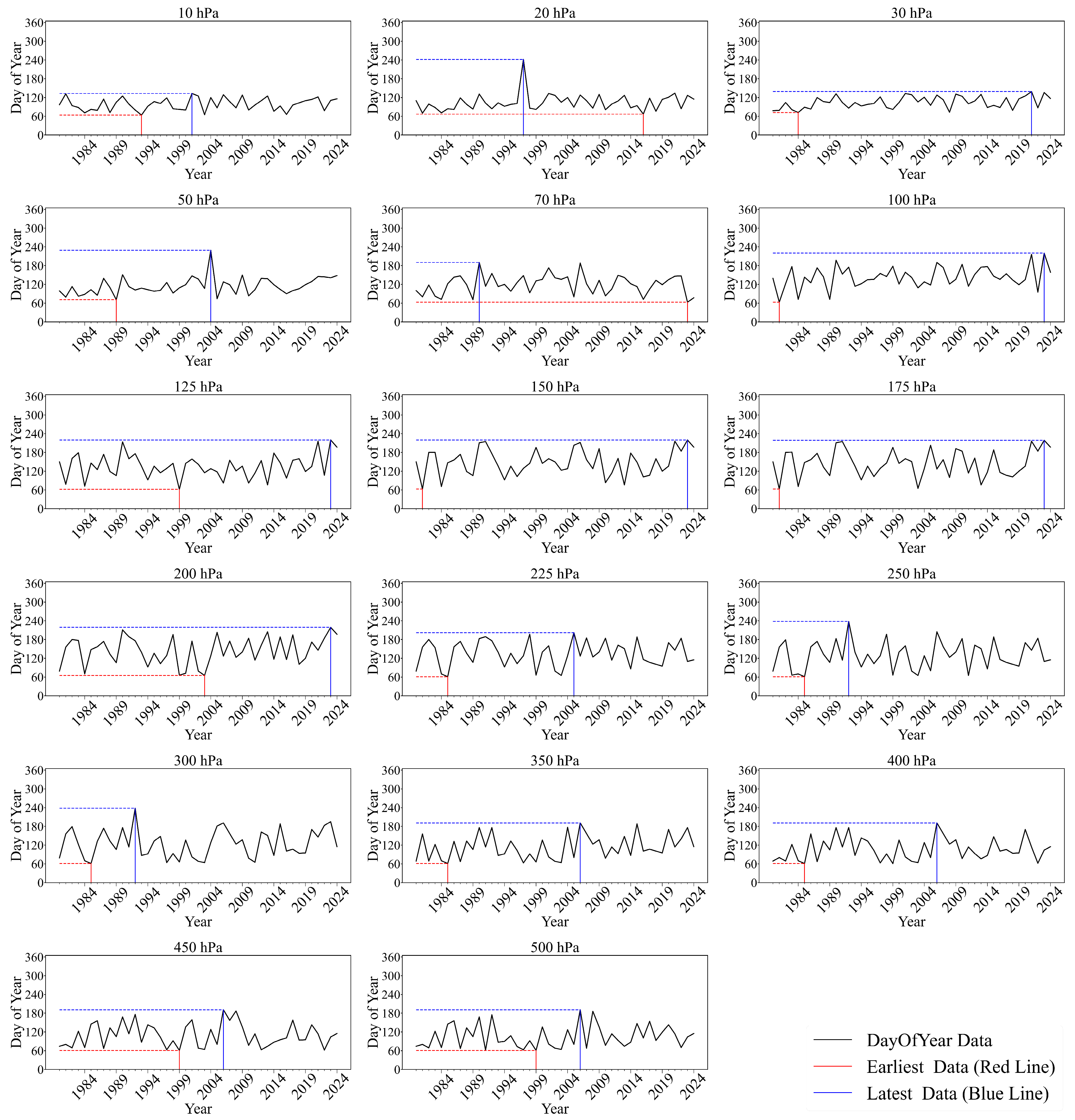
Figure 1 shows the collapse dates of the polar vortex at different heights in the Northern Hemisphere from 1980 to 2024. For the 45-year period, the average collapse date between 10 hPa and 500 hPa is 2 May. The latest average collapse date is 14 July, with the latest collapses occurring around 8 August 2023, at 100 hPa to 200 hPa, and around 10 July 2006, at 350 hPa to 500 hPa. The earliest average collapse date is 4 March, with the earliest collapses occurring around 4 March 1981, at 100 hPa, 150 hPa, and 175 hPa; around 2 March 1985, at 225 hPa to 400 hPa; and around 2 March 1999, at 125 hPa, 450 hPa, and 500 hPa.

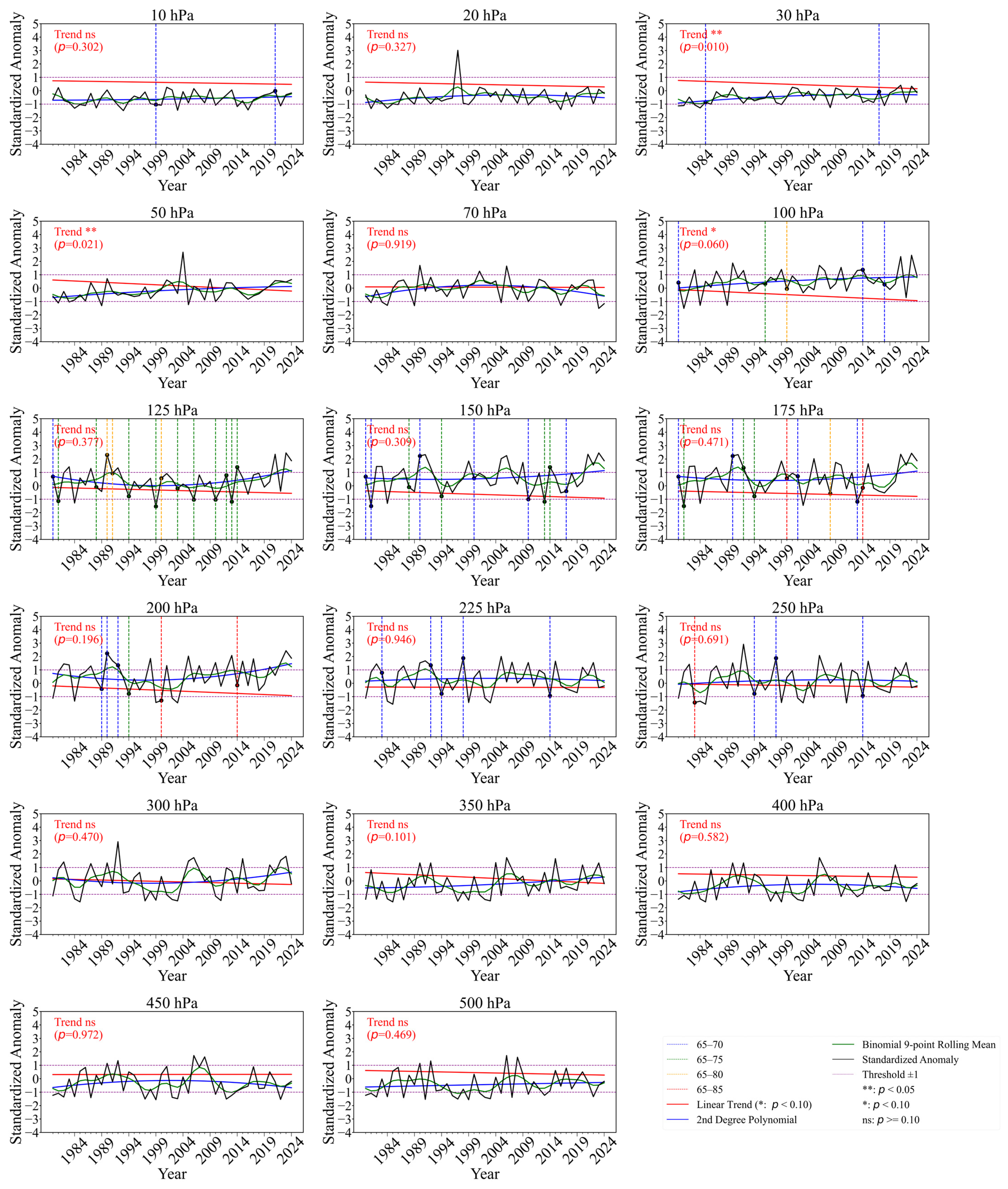
Figure 2 presents the annual variation characteristics of the polar vortex collapse dates in the Northern Hemisphere from 1980 to 2024. We found that for certain height levels and certain years, the collapse signal can only be observed when the latitude range is expanded to 65–70° N, 65–75° N, 65–80° N, or 65–85° N. Therefore, different colored dashed lines are used to indicate this. This is done to better distinguish the differences between the collapse signals. Vertical lines are used to mark the years when the range needs to be expanded in order to capture the signal. This helps to clearly observe the corresponding time of the collapse signals. The different colored dashed lines represent different latitude ranges selected for the calculations. The collapse dates of the polar vortex at various atmospheric levels fluctuate year by year.

The linear trend lines show a significant trend toward earlier collapse dates at the 30 hPa and 50 hPa levels, while the trend at the 100 hPa level is close to significant. For most other layers, the linear trends did not pass the significance test, indicating that their changes cannot be measured with a simple linear trend. The second-order regression line shows that the upper side represents a delayed collapse time, while the lower side indicates an earlier collapse date. It can be observed that the collapse time trends at 125 hPa, 200 hPa, and 300 hPa shifted significantly in 1999, 1993, and 1997, respectively. Before these years, the collapse times generally showed a delayed trend, which subsequently shifted to an earlier trend after these years. In contrast, the collapse time trends at 70 hPa and 450 hPa shifted around 2002. Prior to these years, the collapse times generally showed an earlier trend, which then shifted to a delayed trend after these years. The nine-point smoothing curve also indicates that the collapse dates at other levels did not fluctuate significantly, and the overall changes were relatively stable.

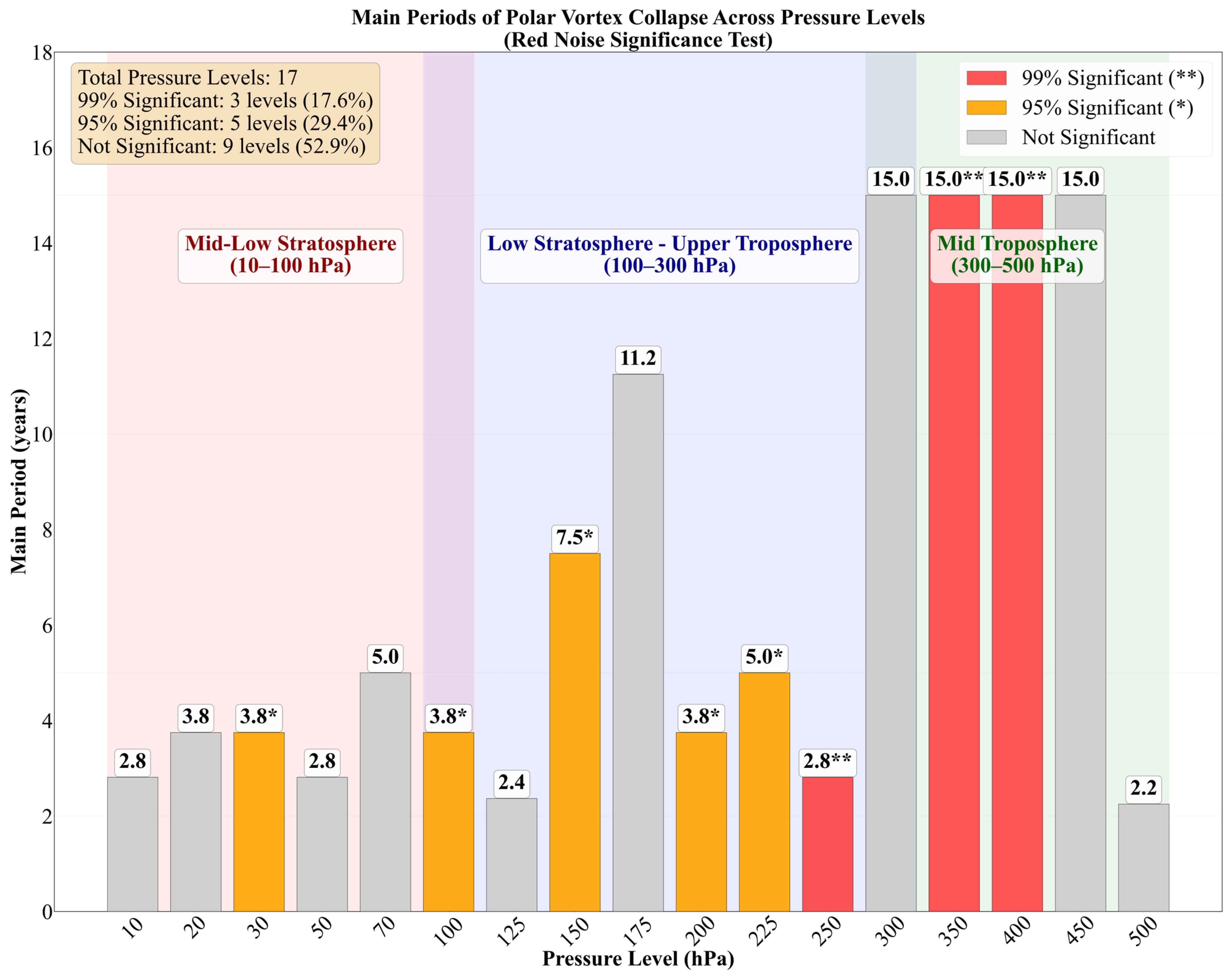
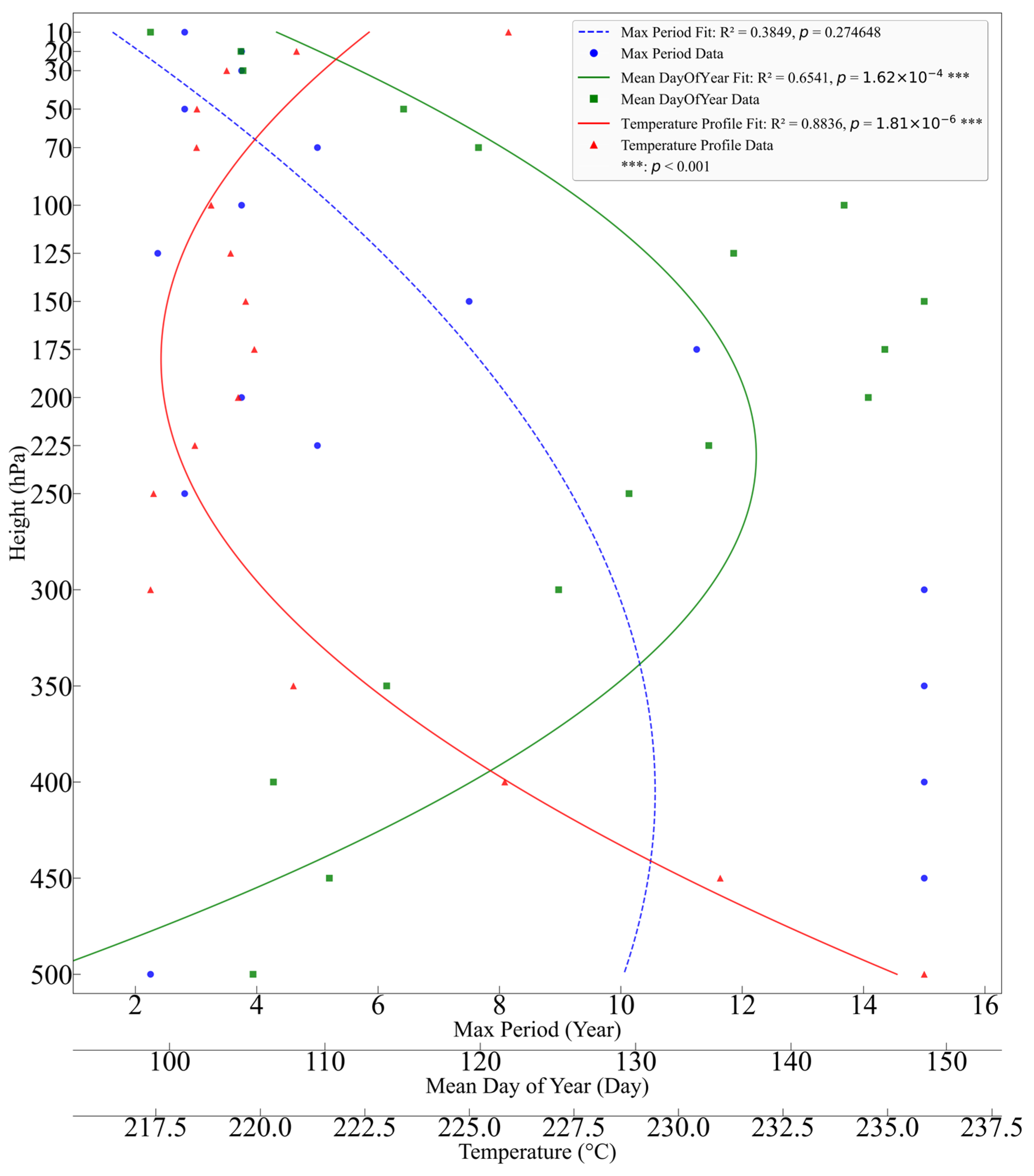
To quantitatively study the periodic characteristics of polar vortex collapse events, we performed Fourier analysis and red noise significance tests on the standardized anomaly time series of collapse dates for each pressure level (10–500 hPa, a total of 17 levels). For each sequence, we first generated 1000 red noise sequences matching the autocorrelation characteristics as the null hypothesis and then calculated the threshold values for the 95% and 99% confidence levels. A period was considered significant if its power exceeded the corresponding threshold. Statistical significance tests were conducted for the main periods at each height. The results show that the periodic characteristics and statistical significance may exhibit a U-shaped structure in the vertical direction (Figure 3 and Figure 4). Specifically, the periodicity of polar vortex collapse exhibits clear vertical stratification: in the lower to middle stratosphere (10–100 hPa), short periods dominate, and the vast majority of signals fail the 95% significance test. The only exception occurs at 100 hPa, where a 3.8-year period is detected and is significant at the 95% confidence level. The lower stratosphere to the upper troposphere (100–300 hPa) is a key region where multiple significant period signals (2.8–7.5 years) coexist. In the middle troposphere (300–500 hPa), there are two robust interdecadal-scale (15-year) oscillations. Notably, the heights of 250 hPa, 350 hPa, and 450 hPa are particularly significant, as they all detected the highest confidence (99% significant) period signals, and future focus can be placed on these levels.

Figure 4 shows that polar vortex collapse events are mainly concentrated in the spring. The green solid line represents the fitted curve of the multi-year average collapse date (day of the year) for different pressure levels, exhibiting a clear quadratic distribution pattern. In the lower to middle stratosphere (10–100 hPa), the collapse occurs earlier, indicating that the seasonal adjustment of the upper atmospheric circulation begins first. In the lower stratosphere to the upper troposphere (100–300 hPa), the collapse time is significantly delayed, especially between 100 and 200 hPa, where fluctuations are notable, making this region the latest for collapse in the vertical direction. In the middle troposphere (300–500 hPa), the collapse time advances again, with a turning point around 400–500 hPa. Overall, the polar vortex collapse shows an “early–late–early” U-shaped evolution in the vertical direction, with earlier collapses in the lower stratosphere and middle troposphere, while the collapse in the lower stratosphere to the upper troposphere (100–300 hPa) occurs the latest.

Year-by-year collapse dates of the polar vortex at different atmospheric levels (Figure S1) indicate that this pattern does not occur consistently every year. For instance, in 1985 and 2019, it exhibited a Z-shaped distribution. Nevertheless, in nearly all of the years, the latest collapse dates were concentrated between 100 hPa and 300 hPa.

The fitted curve of the temperature distribution for different atmospheric layers in the Northern Hemisphere (65–90° N) from 1980 to 2024 is shown by the red solid line in Figure 4, which also exhibits a clear quadratic distribution pattern. The temperature decreases rapidly with altitude in the middle troposphere, between 300 hPa and 500 hPa, resulting in a significant vertical gradient. In the lower stratosphere to the upper troposphere, between 100 hPa and 300 hPa, the temperature continues to decrease, but the gradient begins to weaken. Between 175 hPa and 250 hPa, the temperature increases slightly. As the altitude approaches the tropopause, vertical convection weakens, and the temperature continues to decrease but with a smaller amplitude, forming a gentle slope. Slight warming occurs in the middle and lower stratosphere, between 50 hPa and 100 hPa. In the middle stratosphere, between 10 hPa and 50 hPa, the temperature increases noticeably, forming a distinct stratospheric temperature inversion layer.

Figure 4 reveals the vertical characteristics of the polar vortex in the Northern Hemisphere, highlighting the periodic variations, collapse timing, and thermal structure. These three aspects exhibit strong consistency in terms of their height stratification, as well as clear layered response features. In the middle–lower stratosphere (10 hPa to 100 hPa), the polar vortex had shorter periods and earlier collapse times, as well as a pronounced temperature inversion structure, indicating strong thermal stability controlled by upper-level forcing. In the middle troposphere (300 hPa to 500 hPa), the vortex exhibited the longest periods and relatively early collapse times, with steep vertical temperature gradients. This reflects the rapid response to lower-level disturbances and strong instability. In the lower stratosphere to the upper troposphere (100 hPa to 300 hPa), the period increased abnormally around 150 to 175 hPa, and the collapse times were generally the latest in this zone. The temperature changes exhibited a gentle slope or even localized warming, making this a key anomalous layer for polar vortex activity. Together, these three curves revealed that the polar vortex exhibited nonlinear and asynchronous inter-layer coupling from higher to lower levels. The 100 hPa to 300 hPa range acted as a buffer zone where dynamic disturbances and thermal regulation intersected, playing a critical role in linking the upper and lower layers during the evolution of the polar vortex.

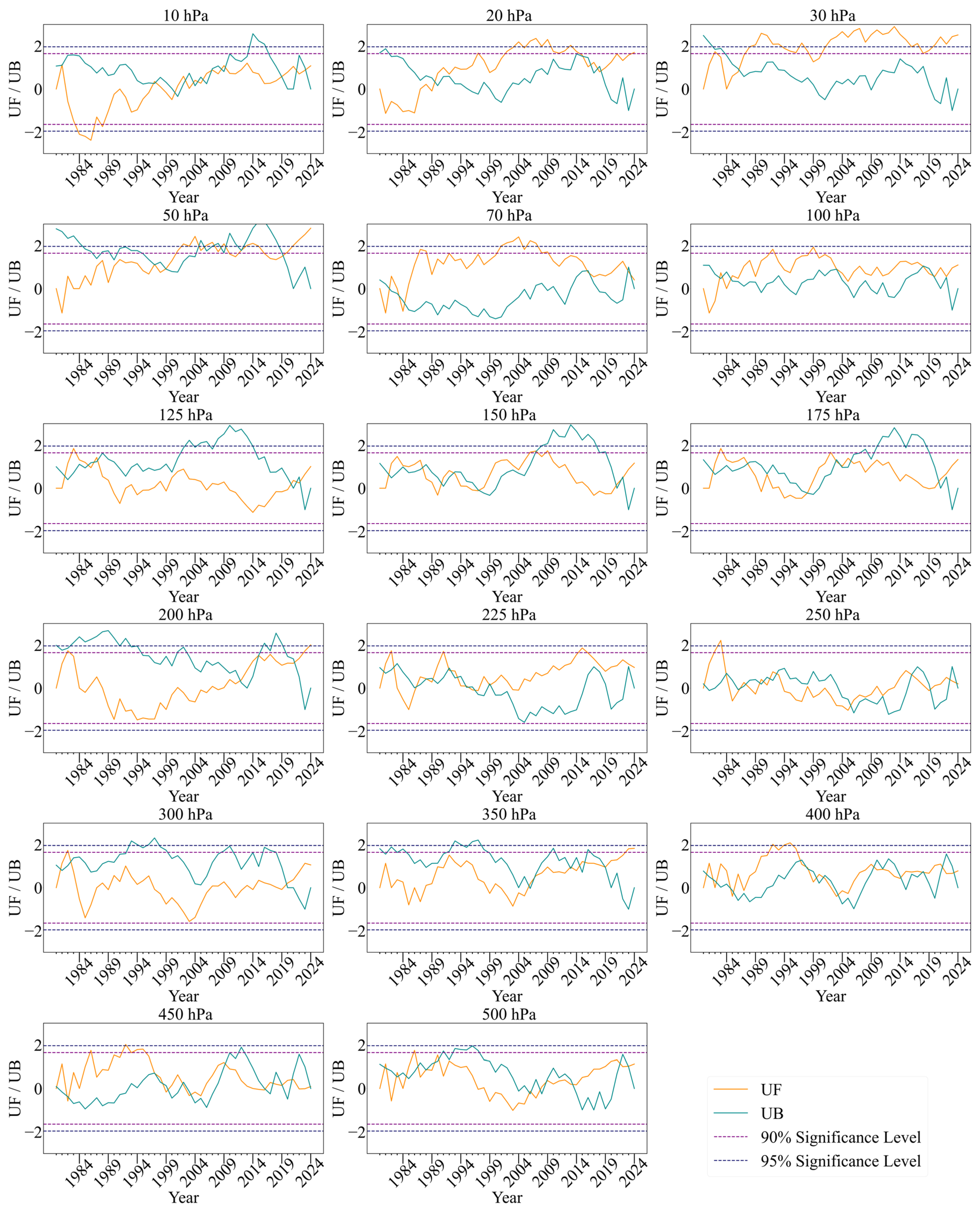
To thoroughly analyze the variability characteristics of the Northern Hemisphere polar vortex collapse dates from 1980 to 2024, this study uses the non-parametric Mann–Kendall (MK) test to detect monotonic trends and change points in the time series. This method is insensitive to non-normal distributions and missing data. The test calculates the statistic (S) by comparing all possible data pairs in the sequence. A positive (S) indicates a potential increasing trend, while a negative (S) indicates a potential decreasing trend. The standardized test statistic (Z) is computed based on (S) and its variance (adjusted for tied values in the data). This study uses a two-sided test and evaluates at two significance levels: (α = 0.05) and (α = 0.01), with corresponding critical (|Z|) values of 1.96 and 2.58, respectively. To identify potential change points, a sequential MK test is further applied, generating the forward statistic sequence (UF_K) and the backward statistic sequence (UB_K). The intersection points of the UF_K and UB_K curves within the confidence bands defined by the two critical lines are considered potential change points [32]. This test is independently implemented at 17 different altitude levels. To control the Type I error rate caused by multiple comparisons, the False Discovery Rate (FDR)/Benjamini–Hochberg method is used for multiple comparison correction at each altitude level. The FDR threshold (q) is set to 0.05. A trend is considered statistically significant for a particular pressure level only when its BH-corrected p-value (p_fdr) is less than 0.05. (The meaning of the p-value is as follows: under the null hypothesis (H₀) that ‘the sequence has no trend’, it represents the probability of observing the current trend strength (or a stronger trend). When the p-value is smaller than the predetermined significance level (α = 0.05), we reject the null hypothesis and conclude that there is a statistically significant trend.).

The variations in the UF (forward sequence) and UB (backward sequence) curves, along with their significance lines and intersection points, were used to determine the statistical significance of trends and identify potential mutation years. Figure 5 presents the UF/UB curves and significance thresholds across all height levels. The dashed line indicates the 95% significance level, used as the primary criterion for determining mutation years; the 90% significance level was also retained for sensitivity analysis to assess the robustness of weaker trend signals. The 90% level is particularly suitable for highly variable interannual phenomena such as polar vortex collapse, as it helps to identify potential weak or emerging trends without altering the main conclusions.

The analysis (in Figure 5) reveals that significant trend variations and mutations are mainly concentrated in the middle–lower stratosphere (10–100 hPa). Below the lower stratosphere and in the upper and middle troposphere (100–500 hPa), the UF curves occasionally exceed the significance threshold, but the UB curves show no coherent behavior, and intersection points are scattered, indicating weak and inconsistent trends without a unified mutation signal. In the middle stratosphere, UF/UB intersections are mainly concentrated between 1981 and 1990, suggesting an overall delay in the polar vortex collapse dates. The lower stratosphere shows a weaker trend but still features identifiable mutation points, notably in 1982 and 1997.

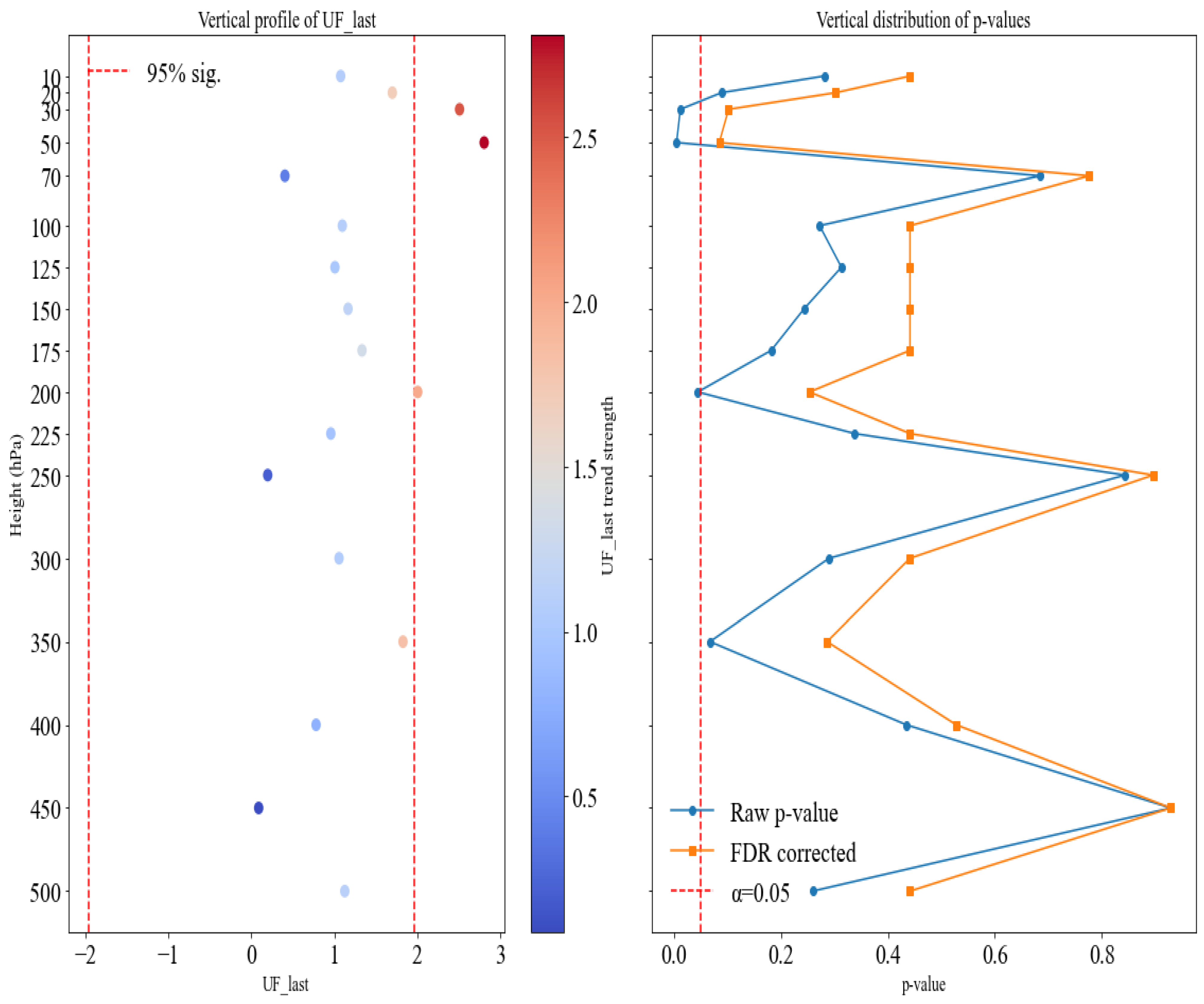
Figure 6 displays the UF_last values and corresponding p-values at each height level, providing an intuitive visualization of the trend significance. Based on the MK test (in Figure 6), the response of polar vortex mutations exhibits clear height dependence: the 50 hPa level shows the strongest signal (UF_last = 2.81, p ≈ 0.005), followed by the 30 hPa level, while both higher (10 hPa) and lower layers (100–500 hPa) display weaker trends (UF_last < 2, p > 0.04). This height dependence can be explained by the vertical sensitivity of wave–mean flow interactions and static stability. Planetary wave breaking does not occur synchronously across altitudes—some disturbances are damped or absorbed in upper or lower layers [25]; the higher layers’ strong static stability inhibits wave propagation, while the lower layers are affected by convective disturbances and turbulent mixing, which further weaken the signal [16]. However, the FDR-corrected p-values for all pressure levels are greater than 0.05, meaning that no trend at any height is statistically extremely significant. Given the limited sample size and interannual variability, although the data exhibit certain changes, these changes did not pass the strict statistical significance test. It is more likely that they reflect the internal natural variability of the climate system rather than a clear, monotonic directional trend.

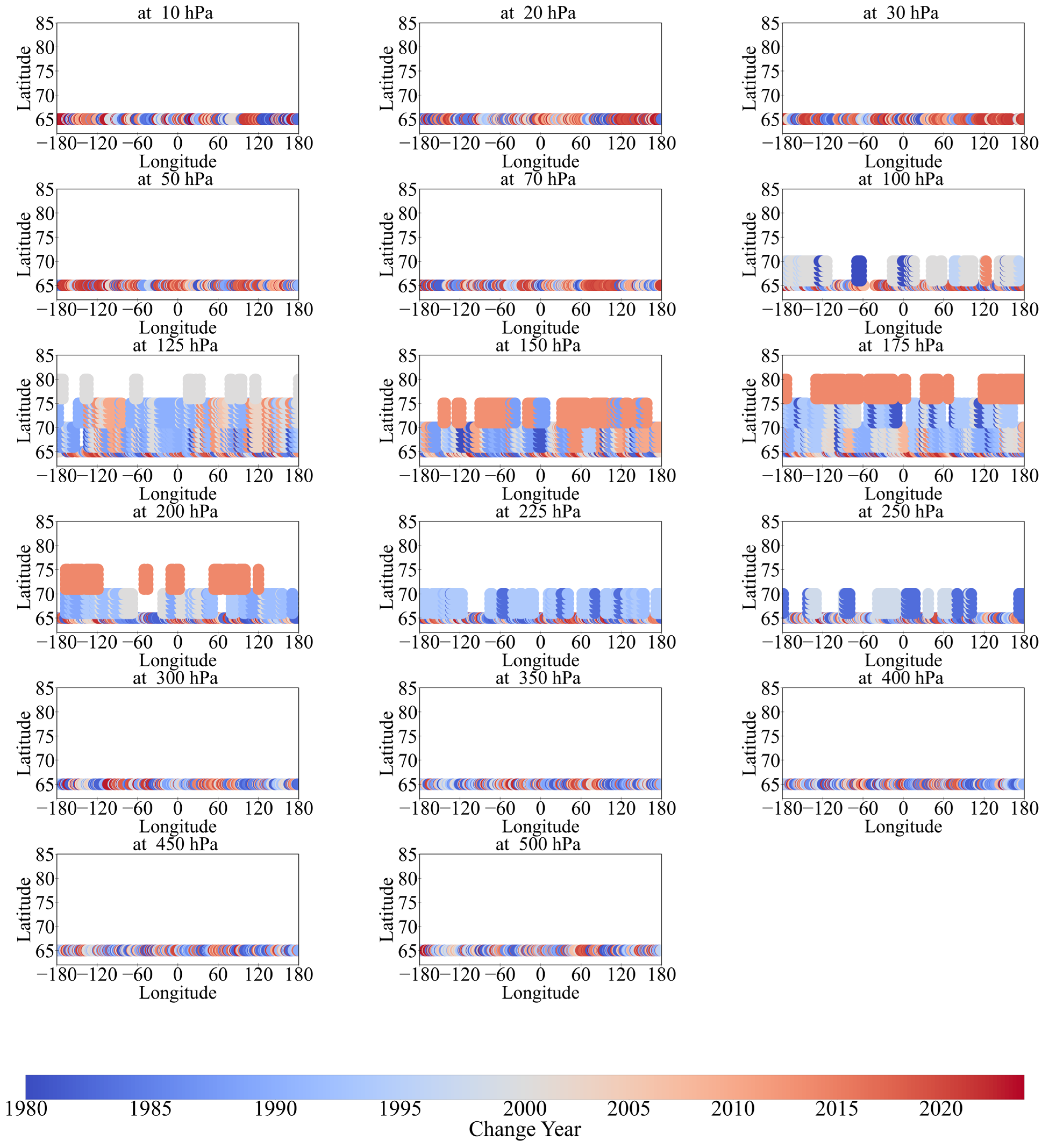
Based on the fact that the collapse signals for certain years at certain altitudes can only be observed when the range is extended to 65–70° N, 65–75° N, 65–80° N, and 65–85° N (Figure 2), and in order to better distinguish the differences between the collapse signals and explore the vertical structural response characteristics of the polar vortex collapse, this study extracts the distribution of change years for different altitude levels during the period from 1980 to 2024 from the Mann–Kendall test results. The focus is on the latitude band of 65–85° N, and the evolution characteristics of the change years in the height–time dimension are analyzed.

The strong and stable polar vortex collapse signal can be captured at 65° N in the 10–70 hPa and 300–500 hPa levels. As can be seen from Figure 7, in the 10–30 hPa range, the shift years, spanning from 2000 to 2015, exhibit a general warm color, indicating relatively late shifts in these levels and suggesting strong latitude concentration of early disturbances in these layers. In the 50–70 hPa, the shift years were mainly within the period from 2005 to 2020, with significant delays at certain longitudes, indicating a spatially phased expansion process. In the 300–500 hPa, the shift years, mostly occurring after 2005, exhibited a delayed response as the upper-level disturbances propagated downward. The response time was later and more spatially concentrated.

In the 100–250 hPa layer, the signal of the polar vortex collapse cannot be detected at 65° N latitude; therefore, the shift points were widely distributed from 65° N to 85° N, especially within 125–200 hPa, forming a distinct belt-shaped shift zone. The shift years spanned from deep blue to deep red, covering the period from 1980 to 2024, and exhibited strong spatiotemporal nonuniformity. This suggests that the result of multiple shift processes or disturbances propagated and accumulated across different regions of the polar region. The shift process of the collapse of the polar vortex exhibited clear vertical temporal hierarchy and spatial latitude concentration (Figure 7).

From the height dimension, the shifts mostly began in the upper and middle stratosphere (around 2000) and then propagated downward to the transition layer and middle troposphere (after 2005). From the spatial latitude dimension, the shifts first appeared near 65°N, gradually expanded to higher latitudes, and eventually formed a continuous shift zone that covered the entire polar region in the 100–250 hPa layer. Therefore, it can be concluded that the interdecadal shifts in the polar vortex structure followed a top-down and edge-to-core propagation path, with 65° N as the source of the shift chain and the 125–200 hPa layer as the region with the strongest shift response. This structure suggests that the changes in the polar vortex may have been closely related to the stratosphere–troposphere coupling mechanism, with significant height-latitude synergistic characteristics.

3.2. Thermodynamic and Dynamic Structural Characteristics of the Collapse of the Polar Vortex

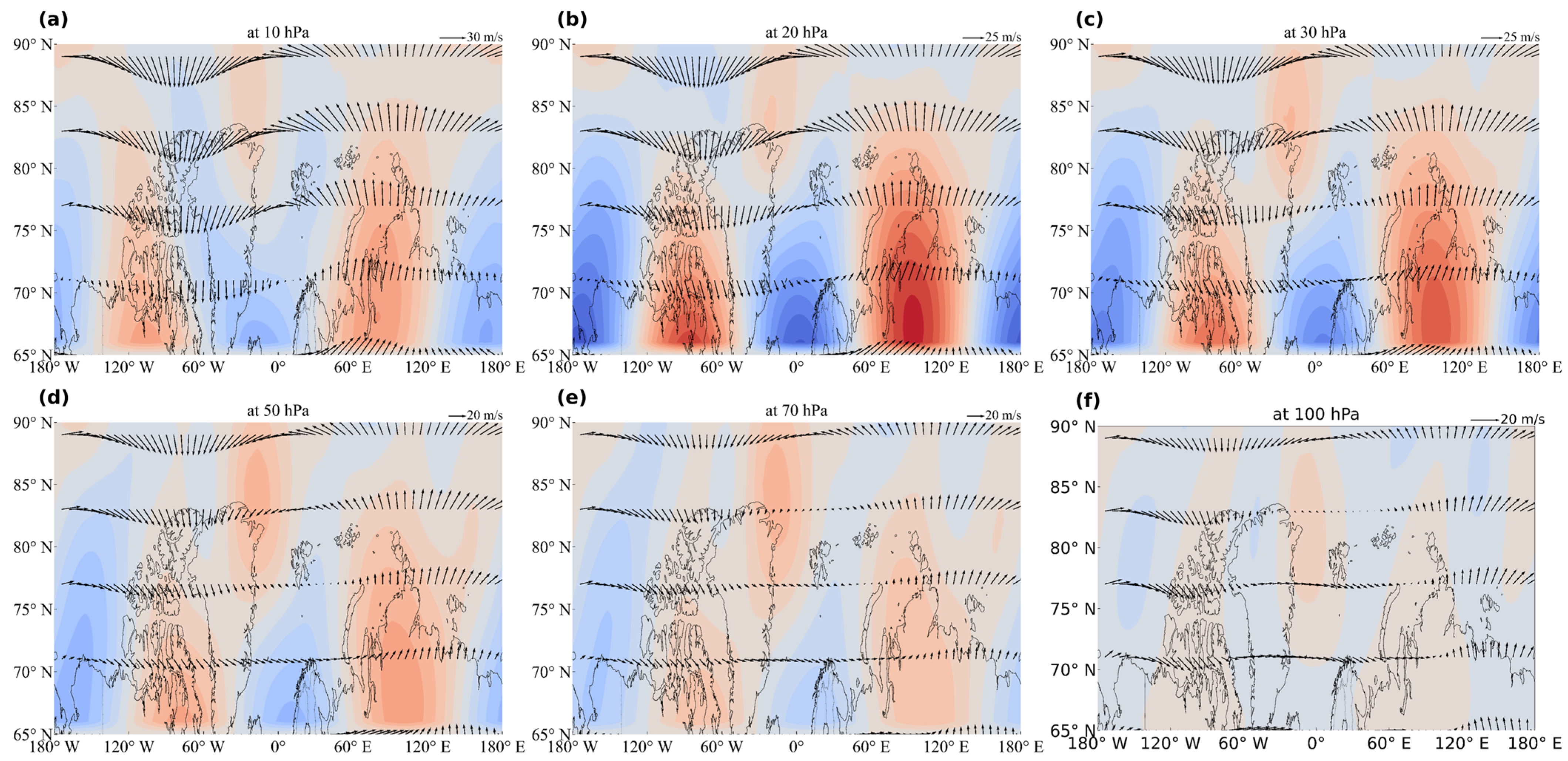
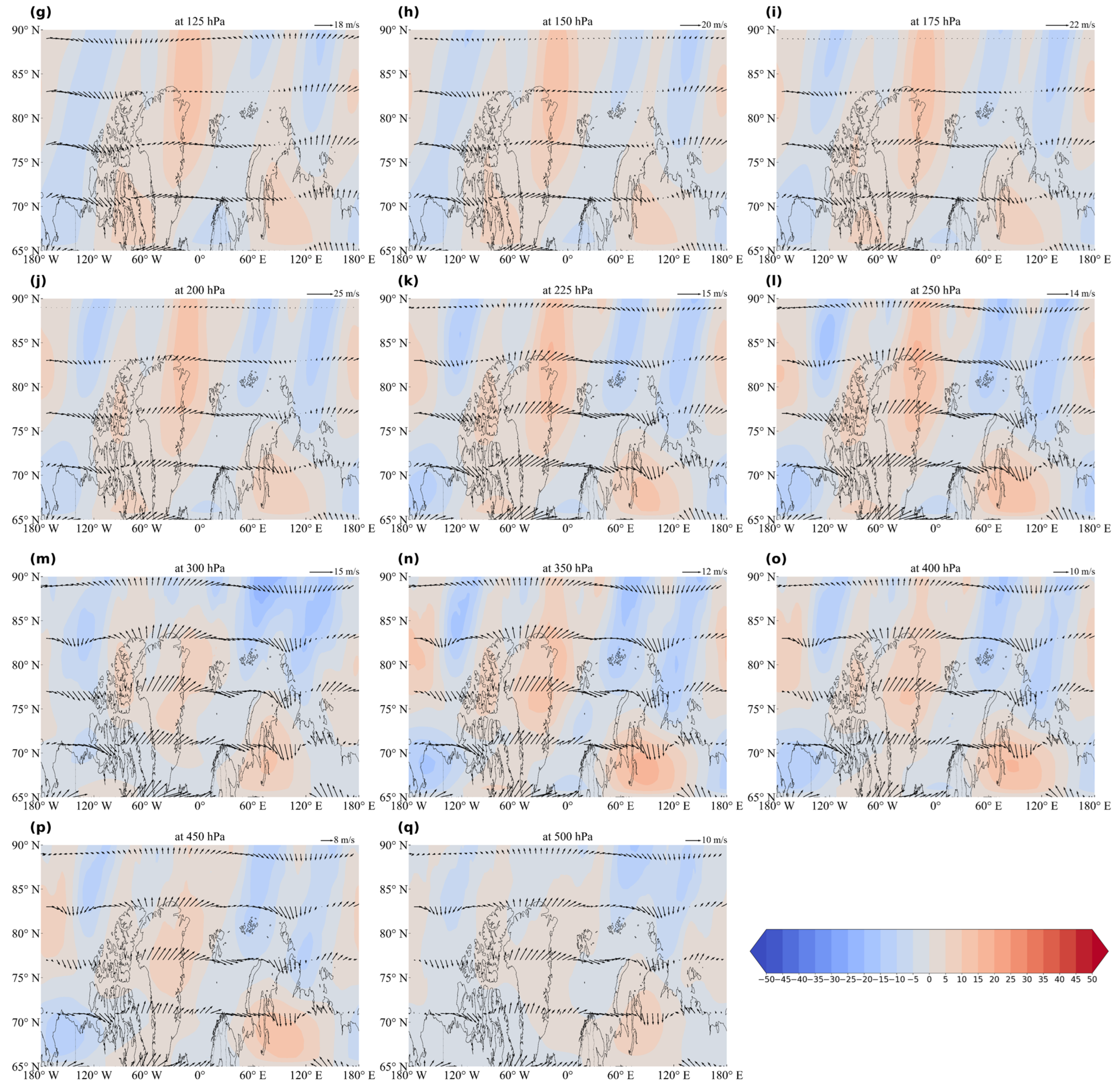
Figure 8 shows that the spatial structure of the momentum flux further evolves in the transition zone from the lower stratosphere to the upper troposphere (100–300 hPa). In the mid-latitude region, particularly over the western North Atlantic and the eastern Pacific region near Japan, a relatively enhanced positive momentum flux is observed, forming two large high-value centers. Although their distribution varies slightly, the overall structure forms a dumbbell-like double-core pattern, located downstream of the Atlantic and Pacific jet stream exit regions. This indicates that this layer is the main area for the release of the stationary momentum flux. Based on zonal wind vector analysis, the direction of the momentum flux is generally consistent with the background westerly winds, extending zonally and expanding toward higher latitudes and toward the east along the exit of the jet stream. This reflects the occurrence of a significant planetary wave–mean flow interaction in this layer, which strengthens the circulation of the polar vortex’s outer region and possibly transfers disturbances to lower layers.

In the middle troposphere (300–500 hPa), the spatial structure of the momentum flux becomes more scattered, exhibiting a fluctuating pattern with alternating positive and negative values, and the overall intensity weakens compared to the upper layers. Only small areas of positive flux occur around Siberia and Greenland. The structure of the zonal wind field becomes more diffuse, and the directions are inconsistent, indicating weakening of the organized momentum transport in this layer.

Figure 8 shows that the stationary momentum flux exhibits typical characteristics of poleward transport and a belt-like distribution in space; vertically, it is stronger at the top and weaker at the bottom structure. This forms a three-tier dynamic coupling process, from stratospheric disturbance to asymmetric breakdown of the polar vortex to tropospheric response, which affects the timing of the collapse of the polar vortex at different height levels. In the middle stratosphere (10–30 hPa), the momentum flux exhibits stable poleward input early on, indicating that this layer starts to receive momentum transport from the mid-latitudes early in the winter. These disturbances continuously weaken the polar region’s circulation, causing the polar vortex to collapse first, and the collapse time is significantly earlier in the upper layers. In contrast, although the transition layer (100–250 hPa) exhibits a dumbbell-shaped positive momentum flux structure, it plays a greater role as a momentum accumulation zone rather than a direct destructive layer. The momentum flux in this layer continues to be transported along the exit of the jet stream, enhancing the disturbance energy. However, due to the stability of the background circulation structure, the disturbances tend to accumulate, diffuse, and redistribute in this layer, resulting in the longest duration of the polar vortex and delayed collapse compared to the upper and lower layers. In the middle troposphere (300–500 hPa), although the momentum flux is limited, its response time to the polar vortex is earlier than in the transition layer due to the layer’s strong response to upper-level disturbances, causing the collapse time of the polar vortex to be earlier in the middle to upper troposphere. Therefore, the U-shaped time distribution structure of the collapse of the polar vortex can be understood to be as follows: the upper layers are most strongly excited by early disturbances, the lower layers respond quickly but briefly, and the middle layers act as a buffer zone for disturbance accumulation and reorganization.

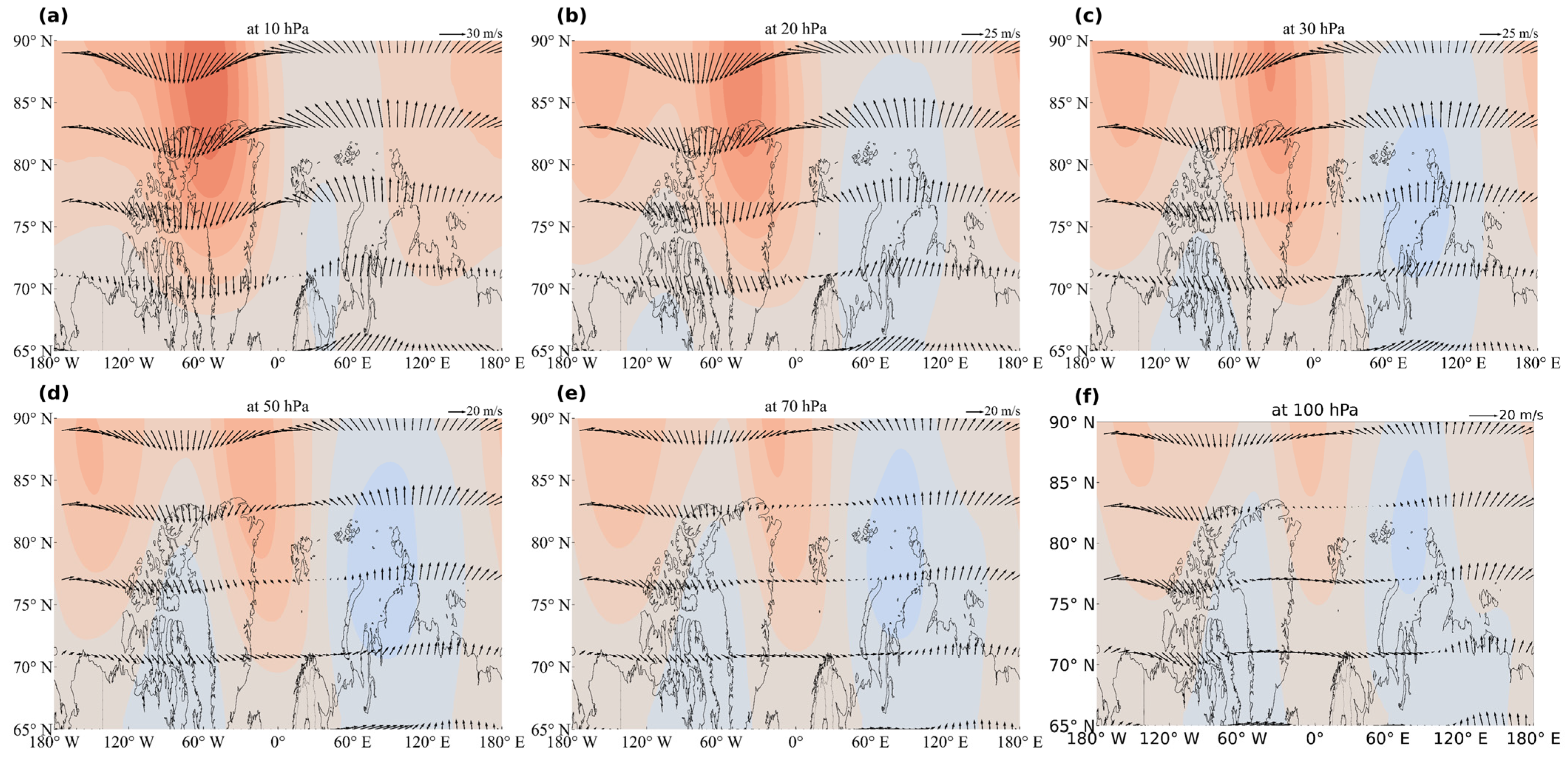
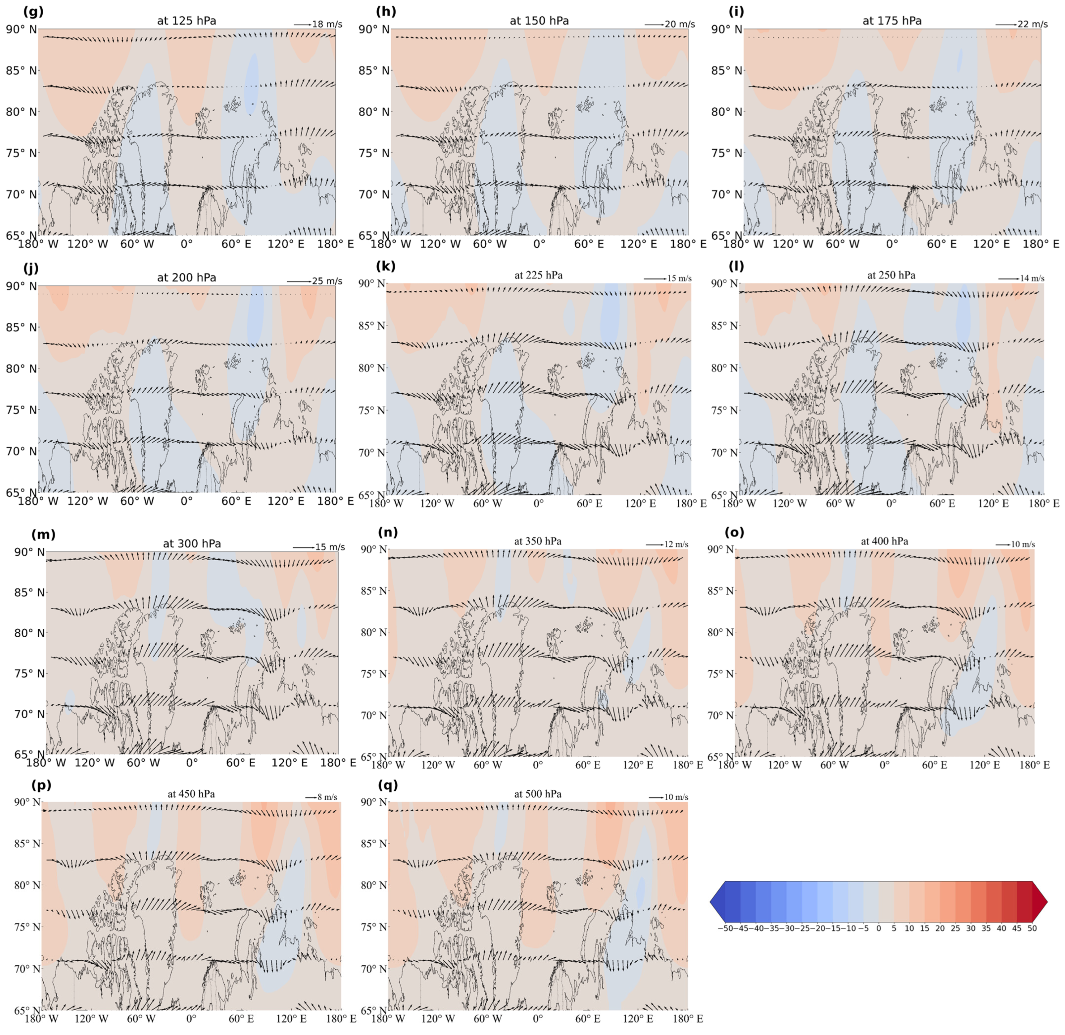
From analysis of Figure 9, it can be seen that in the middle–lower stratosphere (10 hPa to 100 hPa), especially at 10 hPa and 20 hPa, the polar high-latitude region from 65° N to 90° N exhibits a large range of positive stationary heat flux values (warm-colored shading), particularly in regions north of Greenland and near the Chukchi Sea. This significant heat flux intensity indicates clear poleward heat transport and accumulation in this layer. In addition, negative heat flux values (blue shading) mainly occur in the western part of the image (e.g., over the Canadian Arctic Archipelago and the western edge of Siberia), but their intensity is generally weak. There is a clear heat flux gradient band near 65° N, and the zonal wind vectors are oriented from the mid-latitudes toward the poles, reflecting the poleward structure of the heat flux. This suggests that net heat transport from the mid-latitudes to the poles dominates, while the outward heat transport from the polar region is weak or not significant.

In the transition zone from the lower stratosphere to the tropopause (100–300 hPa), the spatial distribution of the heat flux changes. The range of the positive flux within the polar region shrinks, and the overall heat transport weakens. However, in certain mid-to-high latitude regions, such as the western North Atlantic and the eastern Pacific over Siberia, a strong positive heat flux remains, indicating that heat transport from the mid-latitudes to the poles persists in these areas. The flux gradient is more balanced than in the upper layers, and the polar heat accumulation effect weakens. This layer reflects the transition of heat transport to lower layers, indicating weakening of the poleward transport capacity and the beginning of heat transfer to near-surface layers.

The heat flux distribution in the middle troposphere (300–500 hPa) becomes more scattered and complex, exhibiting small-scale alternating positive and negative flux disturbances. The overall structure is less uniform than in the upper layers. In the 65–90° N region, the overall heat flux is weak, but in certain areas (such as eastern Siberia and Northern Europe), localized positive heat flux signals still occur, indicating that heat transport remains functional in these regions. Overall, the heat flux intensity is weaker in this layer than in the middle and upper stratosphere, but it is slightly stronger than in the transition zone, exhibiting a regional disturbance-dominated transport characteristic. The trend of heat accumulation in the polar region is no longer evident at this height.

Heat flux transport plays a key role in weakening the polar vortex, and the collapse timing in the different layers is influenced by the following heat transport characteristics: In the middle–lower stratosphere (10 hPa to 100 hPa), the poleward transport from the mid-latitudes is strongest, with faster warming of the polar region in the upper layers, leading to earlier breakdown of the polar vortex. The collapse in the upper layers is usually the earliest signal of the entire polar vortex collapse process, serving as an important precursor for collapse in the lower layers. The collapse at 50–100 hPa is influenced by the horizontal heat transport in the 100–300 hPa transition layer. Since the heat accumulation in this layer lasts longer and diffuses later, the polar vortex is maintained for a longer period at lower levels, resulting in later collapse. Therefore, collapse generally occurs later in the 50–100 hPa layer than in the 10 hPa layer, but it occurs earlier than in the 100–300 hPa transition zone. In the middle troposphere (300–500 hPa), although the heat flux is weaker, the response time of the collapse of the polar vortex is earlier than in the transition zone due to the response of this layer to upper-level disturbances. In the 100–300 hPa transition zone, the disturbances from the middle troposphere (300–500 hPa) are weaker, and the energy transfer for collapse of the polar vortex is slower, resulting in an increase in the duration of the polar vortex at this level, with collapse occurring later. The collapse in this layer typically occurs in the final stage of the entire collapse process, marking the final result of the downward propagation from the stratosphere.

The conclusions from Figure 9 align with the observation that the polar vortex collapses first in the upper stratosphere and the middle to upper troposphere, followed by the transition zone from the lower stratosphere to the tropopause, exhibiting a U-shaped trend from high to low (Figure 4).

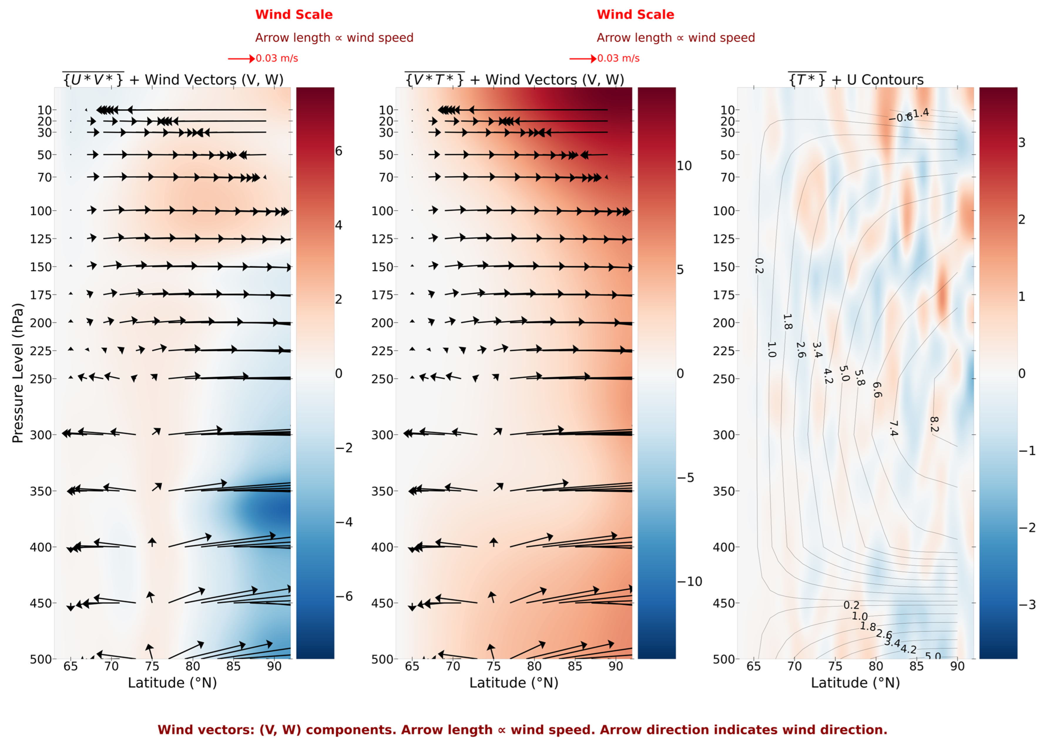
Figure 10 reveals the hierarchical distribution characteristics of the polar vortex collapse time in the vertical and meridional directions, showing the vertical thermal and dynamic structure in the Northern Hemisphere (65–90° N) from 1980 to 2024.

In the middle–lower stratosphere (10 hPa to 100 hPa), both momentum and temperature fluxes are notably enhanced. Between 10 and 30 hPa, zonal wind speeds are relatively low, with zonal southerly winds prevailing in higher latitudes. In the 30–100 hPa range, wind speeds increase with latitude, and zonal northerly winds dominate, with the strongest zonal winds occurring near the polar region. The background color in this region shows strong positive flux, reflecting the significant role of the jet stream in transporting momentum and heat towards the polar region. The closely packed contour lines indicate the onset of polar vortex boundary fluctuations and the breakdown of the upper-level structure.

In the transition zone between the lower stratosphere and the upper troposphere (100 hPa to 300 hPa), changes in zonal wind speed and direction become increasingly pronounced as altitude decreases. Between 75° and 80° N, zonal northerly winds prevail, with relatively strong zonal winds and more stable directions. Between 65° and 75° N, a shift in the circulation occurs—zonal southerly winds appear at 250 hPa, accompanied by significant downward vertical motion. Although momentum flux weakens slightly, positive anomalies persist between 70° and 75° N. In this transition zone, the contours are steeper, and the wave-like structure extends along the latitude direction, facilitating the unstable development of the polar vortex boundary.

In the 65–75° N latitude range, momentum and temperature fluxes in the middle troposphere (300 hPa to 500 hPa) show a marked decrease, particularly in high-latitude areas where the background color shifts to strong negative flux, indicating a weakening of the circulation dynamics. The zonal wind field transitions from southerly to northerly winds from low to high latitudes, with the most pronounced change occurring at 75° N. The temperature field in the high-latitude region is the coldest, with straight and densely packed contour lines, while the zonal wind field intensity increases, suggesting more intense fluctuations at the polar vortex boundary.

The northward transport of warm air driven by the jet stream and the southward movement of cold air create significant temperature anomalies, which enhance atmospheric instability and generate strong vertical motion and energy disturbances. These disturbances initially form in the high-latitude stratosphere, subsequently propagating downward and ultimately affecting the upper troposphere in the polar region, resulting in a three-dimensional circulation disturbance with a U-shaped distribution. This explains why the polar vortex in the Northern Hemisphere first collapses in the middle–lower stratosphere and middle troposphere, followed by collapse in the lower stratosphere to upper troposphere transition zone, exhibiting a U-shaped evolutionary trend from high to low.

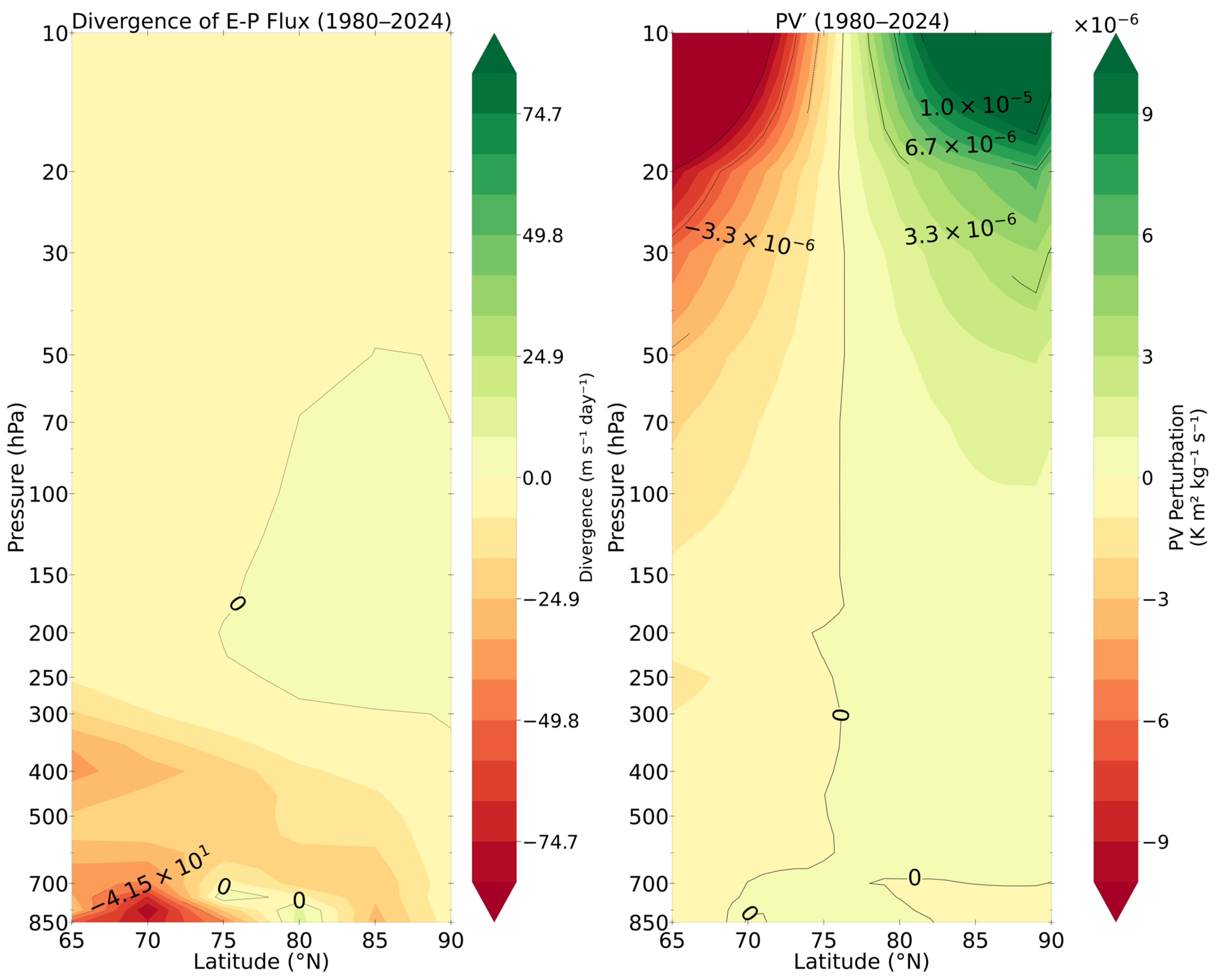
Figure 11 and

Table 1. Statistical Summary of Potential Vorticity (PV) and Eliassen–Palm (EP) Flux in Different Atmospheric Layers.

Level_Range	EP-Mean	EP-Std	Mean (PVU)	Std (PVU)	Variance (PVU2)
10–100 hPa	−0.323450	0.495702	1.39 × 10−4	1.38 × 10−4	1.90 × 10−8
100–300 hPa	−0.665042	3.260586	9.60 × 10−6	3.33 × 10−6	1.11 × 10−11
300–500 hPa	−15.000035	19.790757	1.60 × 10−6	9.00 × 10−7	8.10 × 10−13
500–850 hPa	−25.697717	32.051414	8.34 × 10−7	1.70 × 10−7	2.87 × 10−14

illustrate the vertical–latitudinal structure of the atmospheric dynamical field associated with the polar vortex collapse during 1980–2024.

In the middle–lower stratosphere (10–100 hPa), quantitative analysis shows that the variance of PV disturbances in this layer is 1.90 × 10⁻⁸ PVU², with a standard deviation of 1.38 × 10⁻⁴ PVU, indicating the most significant disturbance intensity. This suggests that the middle–lower stratosphere is a primary source of wave activity. However, when transitioning to the region between the lower stratosphere and upper troposphere (100–300 hPa), the variance of PV disturbances sharply decreases to 1.11 × 10⁻¹¹ PVU², with a vertical decay rate of 99.942%, and the standard deviation drops to just 3.33 × 10⁻⁶ PVU. This drastic energy decay corresponds to a significant weakening of the disturbance gradient, indicating that the polar vortex collapse process encounters intense dynamical buffering as it extends downward into the troposphere.

In the middle troposphere (300–500 hPa), the variance of PV disturbances further decreases to 8.10 × 10⁻¹³ PVU². Although the disturbance characteristics persist, the intensity is only 7.3% of that in the transition layer. Notably, while the EP flux divergence in this layer shows a significant negative value (−15.000 m s⁻¹ day⁻¹), producing strong momentum deposition, the PV disturbances remain relatively weak, forming a “strong momentum forcing—weak vorticity response” dynamical decoupling. This decoupling phenomenon becomes more pronounced in the middle–lower troposphere (500–850 hPa).

In the transition layer (100–300 hPa), quantitative diagnostics reveal key dynamical buffering mechanisms. Although the PV disturbance variance (1.11 × 10⁻¹¹ PVU²) in this layer is smaller than in the stratosphere, it is still greater than in the middle troposphere. Meanwhile, its EP flux divergence is −0.665 m s⁻¹day⁻¹. This “moderate disturbance intensity—low response efficiency” combination forms a unique dynamical feature: wave energy from the stratosphere is partially absorbed and reorganized, but the momentum forcing transmitted downward is significantly weakened. Further analysis shows that the interannual variability of the transition layer (±3.261 m s⁻¹day⁻¹) is only 16.5% of that in the middle troposphere (±19.791), indicating higher temporal stability in this layer. This stability results from a moderate match between PV disturbances and EP responses, which, although insufficient to significantly alter the background flow field, is adequate to form an effective dynamical barrier.

In summary, the physical mechanisms of polar vortex collapse manifest vertically as strong disturbance sources in the middle–lower stratosphere (1.90 × 10⁻⁸ PVU²), buffering in the transition layer, dynamical decoupling in the middle troposphere (strong forcing—weak response), and impacts in the middle–lower troposphere. These stratified features interact through quantified differences in energy transfer efficiency, forming a bidirectional suppression structure where disturbances gradually decay downward from the stratosphere and responses from the troposphere gradually weaken upward. This structure not only delays the onset of the collapse process but also regulates its downward development rate, ultimately shaping the typical U-shaped evolution trajectory observed.

4. Discussion

The methods and conclusions of this study have certain limitations.

Firstly, the 45-year (1980–2024) reanalysis dataset used in this study allows for the analysis of “long-term trends” (with interdecadal variations covering a 15-year cycle). By increasing the sample size, we could achieve a more comprehensive assessment of the stability of large-scale climate events or climate background signals.

Secondly, the core innovation and perspective of this study lie in defining and tracking the collapse of the polar vortex based on the evolution of the zonal wind field, which captures the dynamic core of the polar vortex as a circulation system. However, the results differ from the perspective of collapse events commonly defined in previous studies (e.g., for FFW or SSW), which are based on thermal indicators such as temperature fields. The comprehensiveness of the polar vortex collapse event has not been well represented.

Thirdly, the conclusions of this study are entirely based on the ERA5 reanalysis dataset, which is the most widely recognized and advanced dataset available at this stage. However, in the stratosphere, particularly during the early periods and in regions with sparse high-latitude observations, the field values are highly dependent on model physical parameterizations, which may introduce potential systematic biases.

In addition, although the vertical levels covered in the analysis (10–500 hPa) include both the stratosphere and the main troposphere, which is sufficiently detailed in the ERA5 data, there is slightly insufficient attention to the most complete vertical structure of the stratosphere, including levels such as 0.5–10 hPa. As a result, it is possible that some signals have not been fully captured.

Despite these limitations, this study systematically reveals that the stratosphere–troposphere polar vortex collapse often exhibits a non-uniform, “U-shaped” temporal evolution structure in the vertical direction. This provides a new dynamic framework for understanding the stratosphere–troposphere coupling process. To deepen our understanding and push the boundaries of current research, future work will aim to overcome these limitations and further refine the study of polar vortex collapse events.

5. Conclusions

In this study, based on ERA5 reanalysis data, we integrated criteria for collapse of the polar vortex, the Mann–Kendall test, mutation year extraction, and momentum and heat flux analysis, systematically revealing the spatiotemporal evolution characteristics and causal mechanisms of the collapse of the Northern Hemisphere polar vortex from 1980 to 2024. The main conclusions of this study are summarized below.

From 1980 to 2024, the collapse dates of the Northern Hemisphere polar vortex at different altitudes fluctuated annually, with collapses occurring earlier in the higher stratospheric and upper tropospheric layers and later in the stratospheric lower layers to the tropopause region, exhibiting a U-shaped trend.

The periodicity of the polar vortex collapse exhibits a clear vertical stratification: in the lower and middle stratosphere (10–100 hPa), short-period oscillations dominate, with the vast majority of signals failing to pass the 95% significance test. The only exception occurs at 100 hPa, where a 3.8-year period is detected and is highly significant at the 99% confidence level. The lower stratosphere to upper troposphere (100–300 hPa) is a key region where multiple significant periodic signals (ranging from 2.8 to 7.5 years) coexist. In the middle troposphere (300–500 hPa), a robust interdecadal-scale (15 years) oscillation is present. Notably, the heights of 100 hPa, 250 hPa, and 350 hPa stand out, as all of them detect the most significant periodic signals (99% confidence level).

The polar vortex collapsed in the 10–30 hPa layer first, and the mutation years were concentrated between 1995 and 2005. The collapse then propagated downward to 50–70 hPa, 100–250 hPa, and 300–500 hPa, forming a delayed response chain that spread from high to low altitudes. The spatial distribution of the mutation signal exhibited the characteristics of latitudinal concentration and vertical extension.

The physical mechanisms of polar vortex collapse manifest vertically as strong disturbance sources in the lower stratosphere, buffering in the transition zone, dynamic decoupling in the middle troposphere (strong forcing–weak response), and the influence on the lower and middle troposphere. These vertical characteristics interact through the quantified differences in energy transfer efficiency, forming a bidirectional suppression structure where disturbances gradually weaken downward from the stratosphere and responses weaken upward from the troposphere. This structure not only delays the onset of the collapse process but also regulates the rate of its downward development, ultimately shaping the typical U-shaped evolutionary trajectory observed.