Frame-Based vs. Event-Based Optical Turbulence Strength Estimation: A Comparative and Hybrid Approach

Abstract

Atmospheric turbulence, quantified by the refractive index structure parameter (${C_n}^2$), degrades the performance of optical systems. Reliable ${C_n}^2$ estimation is critical for free-space optical communication, remote sensing, and astronomy. This study compares frame-based and event-based approaches to turbulence strength estimation. A high-speed CMOS camera (180/90/30 frames per second (FPS)) and an event camera were deployed along a 300 m outdoor path, with a scintillometer providing ground truth. Event streams were segmented into 5 s windows, features were extracted, and predictions were made using an Extreme Gradient Boosting regressor (XGBoost). A hybrid model was also tested, combining CMOS-based predictions with event features. Results show that CMOS accuracy is strongly dependent on frame rate, with diminishing returns beyond 90 FPS under weak turbulence. Event-based models achieved higher correlation with ground truth in strong turbulence but produced larger errors in weak regimes. The hybrid approach yielded the best overall performance in moderate-to-strong turbulence, reducing mean estimation error by ~35% compared to CMOS-only at 180 FPS. These findings demonstrate the complementary strengths of frame and event modalities. Frame cameras provide stability in weak turbulence, while event sensors capture fast fluctuations under stronger conditions. Together, they enable more robust ${C_n}^2$ estimation and motivate further research into advanced hybrid sensing strategies for operational turbulence monitoring.

1. Introduction

1.1. Background

Atmospheric optical turbulence is a pervasive phenomenon that imposes fundamental limits on imaging and propagation systems. Turbulence in the air causes random fluctuations in the refractive index, which in turn induce phase distortions and intensity scintillations in optical waves [1]. These effects can severely degrade the performance of various applications: for example, free-space optical communication links suffer increased signal fading and bit errors; long-range imaging and remote sensing systems experience blurring and image dancing; and astronomical telescopes see reduced resolution due to atmospheric seeing. The refractive index structure parameter ${C_n}^2$ is the standard metric for turbulence strength, quantifying the intensity of refractive index fluctuations in the atmosphere [1,2]. Accurate estimation of ${C_n}^2$ along a given path is therefore of great importance for characterizing atmospheric conditions and enabling adaptive optics corrections, link budget planning, and image deblurring in these domains. For instance, in an astronomical adaptive optics system, knowing the current turbulence strength helps in optimizing the wavefront correction strategy, and in a laser communication link, it can be used to adjust error-correction coding or transmit power to counteract expected signal fading [3].

Traditionally, ${C_n}^2$ is measured using dedicated instruments such as scintillometers, which infer path-averaged turbulence strength from the statistical fluctuations of a transmitted optical beam [4]. Scintillometers (e.g., the Scintec BLS series) provide reliable ${C_n}^2$ references and are considered the gold standard in turbulence monitoring [1]. However, such instruments are relatively complex and costly, and they operate separately from imaging systems. Moreover, a scintillometer requires both a transmitter and a receiver positioned at two fixed points in the field, which limits deployment flexibility and makes it impractical to instrument every line of sight [4].

In practice, for horizontal near-ground imaging over long distances, turbulence is often the dominant source of image degradation, and deploying conventional ${C_n}^2$ measurement equipment for every line of sight is impractical [5]. This has motivated the development of optical imaging-based turbulence estimation techniques that can work with ordinary cameras observing a distant scene. This limitation has motivated the development of optical imaging-based turbulence estimation techniques, which require only a single imaging device at the receiver and can operate using arbitrary remote scenes, such as building facades, terrain features, or dedicated targets, without the need for an active transmitter.

One notable approach by Zamek and Yitzhaky (2006) [5] demonstrated that the variance of image irradiance can be related to the local image gradient, enabling estimation of the path-averaged ${C_n}^2$ from a sequence of turbulence-degraded frames [6]. In their method, temporal intensity fluctuations in high-contrast regions of video frames were used to infer turbulence strength, yielding results that showed good agreement with scintillometer measurements [5]. This gradient-based video analysis method and related techniques have laid the groundwork for frame-based turbulence strength estimation. Subsequent studies have extended this concept, using metrics like the temporal power spectrum of image distortions or the variance of apparent image motion to derive turbulence parameters [6], and even employing deep learning to map distorted images to ${C_n}^2$ values [6]. Frame-based methods are attractive because they leverage existing imaging hardware, but their performance may depend on factors such as frame rate, exposure time, and scene content [7].

In parallel with advances in conventional imaging, a new class of bio-inspired event cameras has emerged and shown promise for high-speed vision tasks. Event cameras (also known as neuromorphic or silicon retina sensors) differ fundamentally from standard frame cameras: instead of capturing full images at a fixed rate, they asynchronously record pixel-level brightness changes and output a continuous stream of “events” with microsecond timestamp precision [8,9]. Each event encodes the time, location, and polarity (sign) of a brightness change, which allows the sensor to achieve extraordinary temporal resolution and a very high dynamic range (often around 120–140 dB, compared to ~60 dB for typical CMOS cameras) [10]. Because the sensor output is an asynchronous list of events rather than image frames, conventional computer vision techniques do not directly apply; specialized algorithms are required to extract information from the event stream [10]. Nonetheless, the unique sensing principle of event cameras offers new opportunities in situations where traditional cameras struggle, due to their high speed and dynamic range. Atmospheric turbulence-induced distortions, which can include rapid image dancing (angular jitter) and intensity flickering, are a potential match for the strengths of event-based sensing. Indeed, recent work has started to explore the utility of event cameras in turbulence mitigation. For instance, Liu et al. (2025) proposed an event-guided restoration approach called EvTurb, which leverages high-speed event streams to help separate turbulence-induced blur from geometric distortions in imaging; their framework demonstrated improved removal of turbulence artifacts by using events to decouple these effects [11]. Additionally, some of the earliest experiments combining event and frame data for turbulence scenarios have reported encouraging results. Boehrer et al. (2019) used a neuromorphic event camera alongside a standard camera in a controlled turbulence setting, showing that fusing the event stream with traditional intensity frames can yield sharper and more stable imagery through turbulence [8]. Similar complementary behavior has been observed in other event–frame fusion studies, reinforcing the idea that event-based sensors capture high-frequency dynamics while frame cameras maintain scene structure under mild distortions [10,12]. These preliminary studies suggest that event-based and frame-based information are largely complementary under turbulent conditions: the event sensor excels at capturing high-frequency aberrations, while the frame sensor provides a stable, direct view of the scene even when turbulence distortions are minute. It is worth noting that these prior efforts were primarily aimed at improving image quality under turbulence (mitigation), rather than explicitly estimating the turbulence strength parameter. Thus, the capability of frame and event sensors to directly quantify ${C_n}^2$, and how they compare under identical outdoor conditions, remains to be systematically studied, motivating the present work.

1.2. Motivation

While the above developments indicate the potential of both modalities, several research gaps remain unaddressed:

• Effect of frame rate: Frame-based ${C_n}^2$ estimation methods are well studied, but the impact of camera frame rate on estimation accuracy has not been systematically quantified. Most prior imaging studies have employed video at standard rates (~25–30 Hz); modern high-speed cameras can reach hundreds of hertz, raising the question of how much improvement in capturing turbulence dynamics higher frame rates can provide. It is unclear how much benefit is gained beyond 30 FPS, especially under different turbulence conditions, since this has not yet been rigorously evaluated in the literature. For instance, at 180 FPS each frame is separated by only ~5.6 ms, allowing the capture of faster intensity fluctuations than the ~33 ms frame interval at 30 FPS.
• Event performance in weak turbulence: Event cameras naturally produce fewer events when scene changes are small. In conditions of weak turbulence (i.e., very small wavefront distortions), the paucity of events may degrade the reliability of event-based turbulence metrics. If the medium-induced image changes are subtle, an event sensor could output very sparse data, potentially leading to noisy or biased ${C_n}^2$ estimates. This limitation has not been thoroughly investigated, as prior event-based studies have largely focused on relatively strong turbulence scenarios or qualitative imagery improvements. In extreme cases of a very stable atmosphere, an event camera may register virtually no events for many seconds, yielding insufficient data to estimate turbulence.
• Lack of comparative studies: To date, no comprehensive study has compared frame-only versus event-only approaches for turbulence strength estimation under the same conditions, using a consistent ground truth. The literature contains only isolated demonstrations. For example, event-driven image reconstruction experiments [8] and recent neural network-based turbulence removal using events [11] but a side-by-side performance evaluation of the two sensing modalities (using identical data sets and reference measurements) is missing. Furthermore, a systematic examination of a hybrid strategy that combines frame and event data has not been published in a field setting.
• Need for hybrid inference: Intuitively, combining frame-based and event-based inputs could offer the best of both worlds: the frame camera provides a stable reference image and captures slower or low-amplitude distortions, while the event camera contributes sensitivity to fast, transient features of turbulence. Especially under moderate-to-strong turbulence, an intelligent fusion of these modalities might significantly improve the robustness and accuracy of ${C_n}^2$ estimates. Investigating a simple fusion approach is an important step, as it can provide insight into the potential gains of multi-sensor turbulence monitoring and inform the design of more sophisticated fusion strategies. For example, when turbulence is weak the frame-based method can provide a baseline estimate while the event sensor yields little information, whereas in stronger turbulence the event features can capture rapid fluctuations that complement the frame-based measurements. A fused model could thus maintain high accuracy across a broader range of conditions than either modality alone.

1.3. Objectives

In light of the above gaps, this work aims to evaluate and fuse frame-based and event-based turbulence strength estimation methods. The specific objectives are:

• Frame Rate Analysis: Quantify the effect of frame rate on the accuracy of turbulence estimation by testing a high-speed CMOS camera at 180 FPS and down-sampling the recorded data to equivalent 90 FPS and 30 FPS streams.
• Modal Comparison: Compare the performance of event-based versus frame-based ${C_n}^2$ estimation across multiple atmospheric turbulence regimes (ranging from weak to strong turbulence).
• Hybrid Fusion Feasibility: Assess the feasibility and benefits of a simple hybrid inference model that combines event camera data with frame camera outputs to improve turbulence strength prediction accuracy.

To fulfill these objectives, we conducted an extensive outdoor experiment over an 8-day period. This campaign spanned a range of meteorological conditions and times of day, naturally yielding a broad spectrum of turbulence strengths. A 300 m near-ground optical path was instrumented with a co-located pair of imaging sensors (a high-speed CMOS video camera and a DAVIS-type event camera), as well as a Scintec BLS900 large-aperture scintillometer (Scintec AG, Rottenburg, Germany) that provided continuous path-averaged ${C_n}^2$ measurements as ground truth.

The CMOS camera continuously captured video at 180 FPS (with exposure settings optimized for minimal motion blur), while the event camera simultaneously recorded asynchronous brightness-change events from the same scene. The frame-based model applied gradient-based image processing algorithms to derive ${C_n}^2$ estimates from video sequences, and the event-based model extracted statistical features from 5 s event windows which were then used in an XGBoost regressor.

For hybrid inference, we implemented a straightforward fusion strategy in which the CMOS-based ${C_n}^2$ prediction was appended as an additional input feature to the event-based model. This simple design allows the event-driven predictor to leverage the stability of frame-based estimates in weak turbulence, while simultaneously capturing the fast dynamics provided by event features under strong turbulence. The approach was deliberately chosen as a proof-of-concept to illustrate potential gains; more sophisticated fusion architectures (e.g., deep learning spatiotemporal models) are left for future work [13].

This study is positioned as an initial comparative evaluation of frame-only, event-only, and fused sensing for turbulence strength estimation in a controlled field setting. Our goal is not to exhaustively optimize each algorithm but rather to demonstrate the complementary value of the two modalities and to establish the feasibility of joint inference.

The remainder of this article is organized as follows: Section 2 describes the experimental setup and data processing methodology, Section 3 details the turbulence estimation models, Section 4 presents comparative results and analysis, Section 5 provides a discussion of the findings, and Section 6 concludes the paper with closing remarks and directions for future work.

2. Experimental Setup

2.1. Overview of Setup

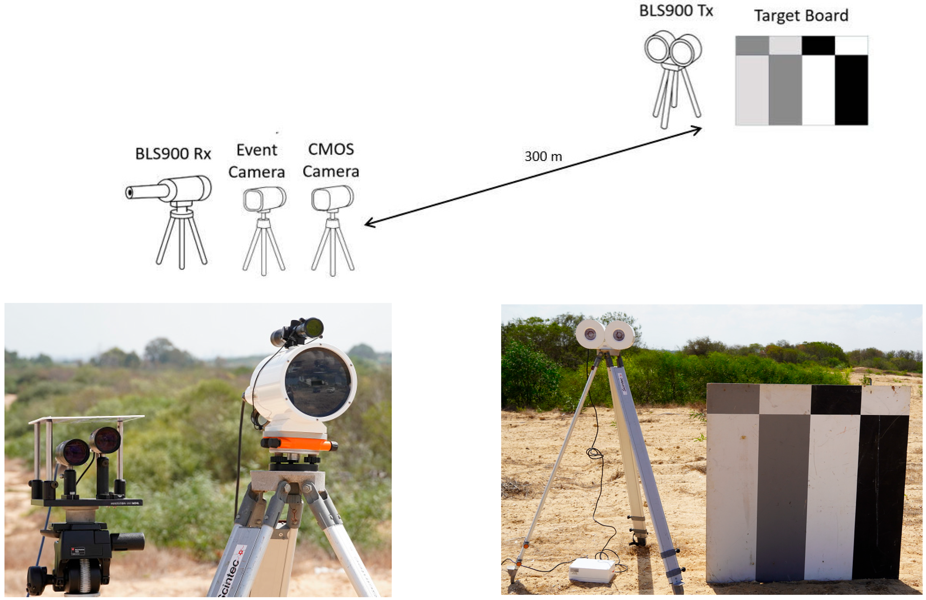
The field experiment was conducted in Yavne, Israel, a coastal-plain location near sea level, using a 300 m horizontal line-of-sight path between a transmitter station and a receiver station (see Figure 1). The transmitter end housed a scintillometer transmitter and a custom target panel (described below), while the receiver end collocated a scintillometer receiver with two imaging sensors: a frame-based CMOS video camera and a neuromorphic event-based camera. The scintillometer was a Scintec BLS900 large-aperture model providing reference measurements of the path-integrated refractive index structure constant (${C_n}^2$). Adjacent to it, we mounted a Basler acA2040-120 um CMOS camera (Basler AG, Ahrensburg, Germany) and a Prophesee Metavision EVK-4 HD (Prophesee, Paris, France) event camera side-by-side, carefully aligned to share the same field of view towards the distant target. This alignment ensured that both cameras and the scintillometer were looking along the exact same turbulence-distorted optical path, enabling a direct comparison of frame-based and event-based observations under identical conditions.

The CMOS camera is a high-speed, 2.2-megapixel global-shutter sensor that was operated at 180 frames per second. Such a high frame rate allowed it to “freeze” fast turbulence-induced distortions in individual frames, a technique that has been used in prior studies of optical turbulence estimation from video [14]. The event-based camera, by contrast, does not capture images at a fixed rate; instead, it asynchronously records individual pixel-level brightness changes as they occur, with microsecond temporal precision [10]. This particular event sensor (Sony IMX636 (Sony Semiconductor Solutions Corporation, Atsugi, Kanagawa, Japan), in the EVK-4 HD) offers an ultra-high dynamic range (>120 dB) and very low latency (sub-100 µs), meaning it can detect rapid intensity fluctuations that a normal camera might miss. Event cameras thus provide a complementary way to sense turbulence: they continuously log the timing and location of intensity changes in the scene, which is well-suited for capturing fast optical distortions (Gallego et al., 2020 [10]). In summary, our setup integrates a traditional imaging sensor and a neuromorphic sensor in parallel, along with the scintillometer, to leverage the strengths of both modalities in measuring optical turbulence.

2.2. Data Acquisition

Data were collected continuously over a one-week campaign from 27 March to 3 April 2025. All three sensors operated 24/7, but for analysis we focus on the daytime hours (07:00–19:00 local time) when the target was clearly visible. During these daylight periods, the atmosphere ranged from morning to mid-afternoon convective conditions (air temperatures ~24–34 °C), providing a broad range of turbulence strengths over the course of the experiment. This yielded approximately 80 h of usable multivariate data (video, events, and scintillometer) under varying levels of optical turbulence. All nighttime data (when low illumination made the target’s contrast too poor for reliable imaging) were excluded from the analysis.

At the receiver station, the BLS900 scintillometer continuously logged a new ${C_n}^2$ measurement every 10 s as the ground-truth reference. Simultaneously, the CMOS camera captured high-speed video of the target at 180 FPS. To manage data rates and align with the scintillometer’s sampling, the camera was operated in a duty cycle mode (recording 50 s of video each minute, then pausing for 10 s) so that each video clip overlapped with multiple scintillometer readings. These short, synchronized bursts ensured that turbulence-induced distortions in the imagery could be directly associated with the scintillometer’s 10 s integrated readings. The event camera, on the other hand, recorded a continuous stream of events with no notion of frames. For subsequent analysis, we segmented this event data into fixed-duration chunks: specifically, we accumulated events into non-overlapping 5 s windows to create frame-like bins of event information. Each 5 s window of event data yields an aggregate representation (such as an event count image or other statistical descriptors) of all brightness changes that occurred in that interval. This fixed 5 s integration time was chosen to be on the same order as the scintillometer’s 10 s output, providing a comparable temporal scale while still capturing sub-sampling fluctuations. In essence, the frame-based camera provides a sequence of intensity images at 180 Hz, whereas the event camera provides a sequence of “event frames” at 0.2 Hz (one every 5 s) after this aggregation step.

The imaging target used in this experiment was a planar contrast panel positioned near the scintillometer transmitter (at the 300 m distant end of the path). This target board featured three distinct vertical stripe patterns of different Michelson contrast levels: a low-contrast pattern (~35% contrast, dark-gray vs. light-gray stripes), a medium-contrast pattern (~45%, dark-gray vs. white), and a high-contrast pattern (~85%, black vs. white). These patterns were designed to test turbulence effects on different image contrasts; however, for the purposes of the present study, we restrict our analysis to the highest-contrast region of the target. In particular, we focus on the vertical black-white stripe pattern (~85% Michelson contrast), as it provided the clearest visual signal of turbulence (strong scintillation and distortion) under all lighting conditions. A fixed Region of Interest (ROI) covering that high-contrast stripe group was used to extract data from both the CMOS frames and the event stream, ensuring that both sensors were analyzing the same physical patch of the target. By using this consistent high-contrast ROI, we maximized the signal-to-noise ratio for turbulence-induced variations and avoided the confounding effects of lower contrast levels.

The high-contrast target panel had an overall size of 1.5 m × 1.5 m. The vertical black–white stripe pattern consisted of stripes of equal width, with each stripe measuring 37.5 cm, corresponding to a black–white spatial period of 75 cm across the target. This geometry defines the dominant spatial frequency content observed by the cameras and directly influences image gradient statistics and event generation efficiency. The selected ROI covered multiple stripe periods, ensuring stable and representative gradient measurements for both the frame-based and event-based analyses.

2.3. Data Processing

All data streams were time-synchronized to enable a direct comparison between the imaging sensors and the scintillometer. The BLS900 scintillometer served as the reference instrument, reporting path-averaged ${C_n}^2$ values every 10 s. Each scintillometer reading was paired with two consecutive 5 s imaging intervals from both the CMOS and event cameras, ensuring that the features extracted from the cameras aligned directly with the ground-truth ${C_n}^2$ values. This one-to-two pairing preserved temporal consistency and avoided any mismatch between imaging windows and the physical turbulence conditions measured along the path.

Next, we extracted quantitative descriptors from the camera data to represent turbulence strength. For the frame-based CMOS data, each 50 s video segment was subdivided into non-overlapping 5 s intervals, processed independently rather than treated as a single long sequence, parallel to the event-camera segmentation. Within each 5 s interval, turbulence-related metrics were derived from the frame sequence, following established image-based turbulence estimation principles [5]. These included measures of apparent image wander, temporal irradiance fluctuations, blur descriptors, and other statistics linked to refractive index variability.

For the event-based data, the asynchronous events were aggregated into the same 5 s windows to generate event-based representations such as event-count images, event-rate descriptors, polarity ratios, and spatial dispersion features. Event cameras, with their microsecond latency and high dynamic range, are particularly well-suited for capturing rapid turbulence-induced distortions that may be undersampled in standard video streams [10]. Each 10 s scintillometer measurement was therefore used to label two consecutive 5 s windows from both modalities, ensuring consistent ground-truth assignment for both the CMOS-based and event-based turbulence descriptors.

Finally, the turbulence-strength estimates obtained from the imaging data were compared to the scintillometer’s ground-truth ${C_n}^2$ values to evaluate accuracy. We employed the Mean Absolute Relative Error (MARE) as the primary error metric. MARE is defined as the mean of the absolute differences between the estimated and true values, normalized by the true values (expressed as a percentage or ratio); it therefore quantifies the average fractional deviation of camera-derived estimates from the scintillometer measurements. A lower MARE indicates that the camera-derived turbulence estimates closely follow the scintillometer readings.

In addition to MARE, we computed the Pearson correlation coefficient between predicted and measured ${C_n}^2$ values. The Pearson coefficient assesses the strength of the linear relationship between the estimated and true turbulence values, capturing how consistently the model tracks fluctuations in turbulence across time. This metric was calculated over the full test dataset (the daytime acquisition periods over eight days) for each method. By using both MARE and Pearson correlation, we quantitatively assessed the performance of frame-based, event-based, and hybrid approaches, providing a robust and complementary basis for comparison in the subsequent Results Section 4.

3. Methods of Turbulence Estimation

In this chapter, we detail the methodologies developed for estimating atmospheric turbulence strength (quantified by the refractive index structure constant ${C_n}^2$) from our multimodal imaging data. Three estimation pipelines are presented: an event-based approach using a neuromorphic event camera (Section 3.1), a CMOS frame-based approach using a high-speed video camera (Section 3.2), and a hybrid fusion approach that combines both modalities (Section 3.3). We also describe the model training and evaluation procedure (Section 3.4).

3.1. Event-Based Prediction

The event camera provides an asynchronous stream of brightness-change events rather than conventional image frames. To leverage this data for turbulence estimation, we segment the event stream into fixed-duration windows (5 s in this study) and extract a comprehensive set of statistical features from each window. The 5 s window length was chosen to balance temporal resolution against noise, roughly matching the scintillometer’s 10 s averaging while still capturing shorter fluctuations (as discussed in Section 3.4). Each 5 s window of events within a given region of interest (ROI) yields one vector of features, which serves as the input to a regression model that predicts the turbulence strength ${C_n}^2$ for that window.

This event-based feature extraction and modeling framework was previously introduced and validated in our earlier work on event-based turbulence prediction [15].

Table 1. Event stream features, formulas, and turbulence rationale.

#	Feature (Name)	Formula	Category	Intuition for Turbulence Estimation
1	Total Events	$N_{evt}$	Temporal	More turbulence $\to$ more brightness changes $\to$ larger $N_{evt}$
2	Positive Event Ratio	${\displaystyle \frac{N_{+}}{N_{evt}}}$	Polarity	Deviation from 0.5 indicates bias in intensity changes
3	Negative Event Ratio	${\displaystyle \frac{N_{-}}{N_{evt}}}$	Polarity	Complement to (2)
4	Max Spatial Span X	$max\left(x\right)-min\left(x\right)$	Spatial	horizontal image wander range
5	Max Spatial Span Y	$max\left(y\right)-min\left(y\right)$	Spatial	Vertical wander range; strongly linked to ${Cn}^2$ [16]
6	Mean Spatial Span X	${\displaystyle \frac{1}{N_{evt}}}\sum (x-\mathrm{m}\mathrm{i}\mathrm{n}(x)$)	Spatial	Average horizontal displacement after offset removal
7	Mean Spatial Span Y	${\displaystyle \frac{1}{N_{evt}}}\sum (y-\mathrm{m}\mathrm{i}\mathrm{n}(y)$)	Spatial	Average vertical displacement after offset removal
8	STD Spatial Span X	${\sigma }_x=\sqrt{{\displaystyle \frac{1}{N_{evt}}}\sum {(x-{\mu }_x)}^2}$	Spatial	Robust spread of x; large under strong turbulence.
9	STD Spatial Span Y	${\sigma }_y=\sqrt{{\displaystyle \frac{1}{N_{evt}}}\sum {(y-{\mu }_y)}^2}$	Spatial	Robust spread of y; large under strong turbulence.
10	Event Rate (MEvt/s)	${\displaystyle \frac{N_{evt}}{{10}^{6}T}}$	Temporal	Normalizes count by window length T (T measured in µsec)
11	XY Correlation	${\rho }_{xy}={\displaystyle \frac{cov(x,y)}{{\sigma }_x{\sigma }_y}}$	Spatial	Detects diagonal shear in displacements
12	XT Correlation	${\rho }_{xt}={\displaystyle \frac{cov\left(x,t\right)}{{\sigma }_x{\sigma }_t}};$ ${\sigma }_t=\sqrt{{\displaystyle \frac{1}{N_{evt}}}\sum {(t-{\mu }_t)}^2}$	Temporal	Horizontal drift trend vs. time
13	YT Correlation	${\rho }_{yt}={\displaystyle \frac{cov(y,t)}{{\sigma }_y{\sigma }_t}}$	Temporal	Vertical drift trend vs. time
14	Spatial Event Density	${\displaystyle \frac{N_{evt}}{(max\left(x\right)-min(x\left)\right)(max\left(y\right)-min(y\left)\right)}}$	Spatial	Distinguishes dense scintillation from sparse wander
15	Spatial Entropy (32-bin)	$-{\displaystyle \sum _{i=1}^{32}}{p}_i\mathrm{l}\mathrm{o}\mathrm{g}\left(p_i\right)$	Spatial	Uniform scatter (high entropy) ⇔ strong turbulence
16	Inter-Event Mean	$\overline{∆t}={\displaystyle \frac{1}{N_{evt}-1}}\sum {∆t}_i$	Temporal	Shorter mean gap = faster fluctuations
17	Inter-Event STD	${\sigma }_{∆t}=\sqrt{{\displaystyle \frac{1}{N_{evt}-1}}\sum {({∆t}_i-\overline{∆t})}^2}$	Temporal	Variability of event timing
18	Inter-Event Median	$\mathrm{M}\mathrm{e}\mathrm{d}\mathrm{i}\mathrm{a}\mathrm{n} \mathrm{o}\mathrm{f} {∆t}_i$	Temporal	Robust central gap measure
19	Spatial Dispersion	$\sqrt{{{\sigma }_x}^2+{{\sigma }_y}^2}$	Spatial	Net 2D jitter; analogous RMS spot size

Variable definitions, $x,y$: pixel coordinates of each event inside the ROI. $t$: event timestamps (µs). $N_{evt}$: total number of events; $N_{+}{N}_{-}$: count of positive/negative events. ${\mu }_x,{\mu }_y$: means of $x-\min \left(x\right)$ and $y-\mathrm{m}\mathrm{i}\mathrm{n}\left(y\right)$. ${∆t}_i$: consecutive inter-event intervals within the window. $p_i$: probability of mass in the $i^{th}$ spatial bin for entropy. T: integration-window duration.

lists the 19 features computed from each event window, along with their formulas and physical interpretations for turbulence. These features capture various aspects of the event distribution in time and space, aimed at characterizing turbulence-induced image distortions. In general, intensity scintillation (rapid brightness fluctuations due to turbulence) will produce a high rate of events, whereas image wander or distortions (slow drift or warping of the target image) will reflect in the spatial distribution of events. Features are therefore grouped as Temporal, Spatial, or Polarity-based measures. Temporal features (e.g., event rate, inter-event timing statistics) quantify the frequency and timing of brightness changes; spatial features (e.g., spatial span, dispersion, correlations) describe the geometric spread and pattern of event locations; polarity features distinguish contrast increases vs. decreases. By capturing both the temporal flicker and spatial jitter signatures of turbulence, the feature set provides a rich description of the underlying refractive perturbations.

Using these features, we trained a regression model to predict the turbulence strength. We selected the Extreme Gradient Boosting method (XGBoost) for this task, as it is a powerful tree-boosting regression algorithm known for its efficiency and accuracy in capturing nonlinear relationships [17]. The XGBoost regressor takes the 19-dimensional feature vector from each event window and learns to output a corresponding ${C_n}^2$. We justified using XGBoost due to its ability to handle diverse feature scales and its built-in feature importance metrics, which provide insight into the most informative event features. The use of a machine learning model (as opposed to an analytical formula) is motivated by the complexity of turbulence effects on the events—by learning from training data (paired with ground-truth scintillometer measurements), the XGBoost model can automatically weigh the features and capture interactions that correlate with turbulence strength.

After training the event-based model, we evaluated the relative importance of each feature in the XGBoost predictor. Notably, a subset of features emerged as most influential. In particular, Total Events, Inter-Event STD, Positive Event Ratio, Mean Spatial Span Y, and Event Rate were the top five contributors, together accounting for roughly 45% of the model’s explained variance. This indicates that turbulence-induced increases in event count and flicker variability, as well as changes in event polarity balance and vertical displacement (Corresponding to the selection of the ROI that contained a vertical line), are strong predictors of the refractive index structure parameter in our data. These results make physical sense: more intense turbulence causes more frequent brightness changes (hence more events and higher event rate), more irregular timing (high inter-event STD), and can introduce biases in brightness change polarity (if, for example, the scene tends to brighten or dim overall under certain distortion). The prominence of Mean Span Y aligns with the expectation that vertical image wander (e.g., dancing of the target up/down) is strongly correlated with turbulence strength in a near-ground horizontal path. Overall, the feature importance analysis validates that the event camera is capturing meaningful turbulence signatures.

The use of an event-based sensor offers key advantages for turbulence measurement. Unlike frame-based cameras, event cameras operate with microsecond-scale temporal resolution and high dynamic range, allowing them to detect rapid, subtle brightness fluctuations without blur or saturation [10]. Atmospheric turbulence can induce very fast intensity scintillations and edge fluctuations that a 180 fps frame camera (5.5 ms frame interval) might miss or blur. In contrast, the neuromorphic event camera continuously registers changes as they occur, effectively “sampling” the turbulence in real-time. Additionally, the event stream is sparse and focuses only on changes, which is well-suited to capturing the moving distortion patterns (the “boiling” effect of turbulence) against a high-contrast target. Prior works have highlighted these benefits of event cameras for high-speed, high-dynamic-range vision [10], and our results similarly suggest that event-based sensing is a promising approach for optical turbulence monitoring [5]. By leveraging these advantages with appropriate feature extraction and machine learning, the event-based model can provide a fast, sensitive estimate of $\widehat{{{C_n}^2}_{EVENT}}$ from the raw event data.

3.2. CMOS-Based Prediction

In parallel with the event-based approach, we implemented a frame-based turbulence estimation method using the high-speed CMOS video camera. The CMOS camera captured intensity images of the target at 180 frames per second, effectively “freezing” much of the turbulence-induced distortion at each frame. To explore the impact of frame rate on turbulence estimation, we also tested the method after subsampling the video stream to 90 fps and 30 fps (by skipping frames) in our experiments. This allowed us to assess how well a standard camera would perform at lower sampling rates. However, unless otherwise noted, the description here assumes the full 180 fps data. Each 5 s video clip (roughly 900 frames at 180 fps) is processed to produce one turbulence strength estimate.

We employ the method proposed by Zamek and Yitzhaky [5] for estimating turbulence strength from an arbitrary set of atmospherically degraded images. The method is based on the relation between the angle of arrival (AOA) of light and the spatiotemporal movements across the frames of the image set (also called “image dancing”).

The analysis of the image displacement single-axis variance ${\sigma }_{img}^2$ of the set of images over time is accomplished by calculating the local temporal intensity variance ${\sigma }_I^2\left(m,n\right)$ and by calculating the gradient square at pixel $\left(m,n\right)$, where the gradients $I_x$ and $I_y$ are calculated over the averages set of images:

$${\sigma }_{img}^2\left(m,n\right)={\displaystyle \frac{{\sigma }_I^2\left(m,n\right)}{\left[I_X^2\left(m,n\right)+I_Y^2\left(m,n\right)\right]}},$$

(1)

On the other hand, the theoretical relation between the AOA fluctuations and the displacement variance (${\sigma }_{img}^2$) is given by:

$${\sigma }_{img}^2\left(m,n\right)=PFO{V}^{-2}·D^{-1/3}·L·C_n^2·P,$$

(2)

where $PFOV$ is the pixel field of view, $D$ is the aperture diameter, $L$ is the path length, $P$ is defined as:

$$P\equiv \left\{\begin{array}{c}2.914, l_0\ll D\ll \sqrt{\lambda L}\\ 1.1, \sqrt{\lambda L}\ll D\ll L_0\end{array},\right.$$

(3)

With $l_0$ and $L_0$ denoting the turbulence inner and outer scales, respectively, and $\lambda$ the wavelength. To simplify, we assume $C_n^2$ is constant along the imaging path.

Combining these relations, the per-pixel estimator of turbulence strength becomes:

$$C_n^2\left(m,n\right)={\left(\left[I_X^2\left(m,n\right)+I_Y^2\left(m,n\right)\right]·L·P\right)}^{-1}·PFO{V}^2·D^{1/3}·{\sigma }_I^2\left(m,n\right),$$

(4)

In practice, the estimation is not calculated for every pixel but only for those where the gradient magnitude is sufficiently large. The final turbulence strength estimate is then given by averaging over $N$ such pixels:

$$C_n^2={\displaystyle \frac{\sum _{m,n}{C}_n^2\left(m,n\right)}{N}},$$

(5)

This CMOS-based model is entirely deterministic, representing a direct physics-based calculation rather than a learned model. No machine learning predictor was trained on the frame data; instead, the above equations were applied to each 5 s video segment to produce an estimate. The method, derived from first principles and empirically validated in prior literature [5], makes it a robust baseline. In our implementation, we calibrated the pixel field-of-view (PFOV) using camera optics and geometry, and used the known aperture size D = 0.15 m and path length L = 300 m. The CMOS method thus produces an estimate $\widehat{{{C_n}^2}_{CMOS}}$ every 5 s, to be compared with scintillometer ground truth. Because it does not learn from data, the performance of this method depends on how well the assumptions (small distortions, constant ${C_n}^2$ along the path, etc.) hold in our scenario.

3.3. Hybrid Inference

While the event-based and CMOS-based estimations each have merit on their own, we also explored a hybrid fusion approach to combine the strengths of both modalities. The hybrid strategy we employ is a form of late fusion at the feature level: we use the CMOS-derived turbulence estimate from Section 3.2 as an additional input feature to the event-based model. In practice, for each 5 s window (ROI), we first compute the deterministic $\widehat{{{C_n}^2}_{CMOS}}$ using the gradient-based algorithm. We then append this value to the 19-dimensional event feature vector (Table 1) for that same time window, creating a 20-dimensional augmented feature vector. We train a new XGBoost regressor that takes these augmented features and outputs the fused turbulence prediction $\widehat{{{C_n}^2}_{hybrid}}$.

Crucially, the original event feature definitions and ordering were preserved; the only difference is the inclusion of one extra feature (the CMOS estimate—$\widehat{{{C_n}^2}_{CMOS}}$). This scalar fusion allows the machine learning model to learn how to weight the CMOS prediction relative to the event features. If the CMOS estimate is accurate, the model can choose to rely on it heavily; if it has biases or errors under certain conditions, the model can learn to adjust or even ignore it in favor of event features. We emphasize that this is a proof-of-concept fusion: it does not involve deep integration (e.g., no joint processing of raw event data and images, but rather combines the outputs of the two separate pipelines at a high level.

The motivation for the hybrid model is that the event and frame sensors respond to turbulence in different ways, especially under varying conditions. For instance, under weak turbulence, the distortion of the image might be too small to trigger many events (since the event camera has a threshold for brightness change), whereas the CMOS method, averaging over many frames, might still detect a slight wander. Conversely, under very strong turbulence, the CMOS images might become too blurred or the gradient method assumptions might break down, whereas the event camera could still fire intensely and capture the fast scintillations. By fusing the two, the hybrid model can, in principle, cover each other’s weaknesses and produce a more robust estimate across the full range of conditions.

After training the hybrid XGBoost regressor, we examined the feature importance to see how much the model utilized the CMOS-derived input. We found that the single CMOS-based ${C_n}^2$ feature contributed approximately 35% of the total feature importance in the hybrid model—by far the largest share for any individual feature. In other words, the learned model tends to trust the physics-based CMOS prediction significantly, adjusting it using the event features. This influence was most pronounced in low-turbulence scenarios: when turbulence was weak (and event activity sparse), the CMOS estimate often provided a baseline signal, and the model leaned on it to make an informed prediction. Under higher turbulence, the event features carried more weight (since they robustly signaled intensity flicker and image motion), but even then, the CMOS feature remained among the top contributors (~35% overall importance). The fact that the CMOS feature is not 100% (i.e., the hybrid model does not just “copy” the CMOS result) indicates that the event features are indeed providing complementary information and the regressor is combining them to improve accuracy.

We stress that our hybrid approach is a late fusion proof-of-concept rather than an optimally tuned multi-modal network. In a late fusion scheme, the two modalities are processed mostly independently up to a final combination stage (here, concatenation of features). This is in contrast to an early fusion or a deep integrated model that might, for example, train a neural network to jointly ingest event data and image data (e.g., [18,19]). Our goal here was to demonstrate that even a simple fusion at the decision level can yield benefits: by injecting the CMOS prediction as an additional feature, the event-based model’s performance improved, especially in regimes where one sensor had an advantage. The success of this approach (as shown in Section 4 results) suggests that a more tightly integrated fusion (e.g., a learned model combining raw data streams) could further enhance turbulence estimation, although developing such a model was beyond the scope of this work. Nonetheless, this late-fusion model serves as a step toward multimodal turbulence inference, showing the value of combining neuromorphic vision with conventional imagery for atmospheric sensing.

3.4. Model Training and Evaluation

3.4.1. Training Procedure

We trained and evaluated the machine learning models (the event-only model from Section 3.1 and the hybrid model from Section 3.3) using a rigorous cross-validation procedure, while the CMOS-based method (Section 3.2) does not involve learning. Both the event and hybrid models were trained to regress the scintillometer-measured ${C_n}^2$ (ground truth) from their respective input features. To make the best use of our data and to assess generalization, we employed K-fold cross-validation with $K=5$ folds. The entire timeline of the experiment (spanning ~80 h of daytime data) was partitioned into 5 folds (each roughly ~16 h of data). In each fold iteration, one fold (time block) was held out for testing while the model was trained on the remaining four folds; this was repeated so that each fold served as the test set once. Importantly, the folding was performed chronologically (by contiguous time blocks) rather than randomly shuffling windows, to prevent any temporal leakage [20]. Temporal leakage is where training and testing samples from nearly the same time period could be correlated what would be especially problematic in our scenario because turbulence has diurnal cycles and short-term correlations. By using time-separated folds, we ensure that the model is evaluated on truly unseen conditions, providing a more robust indication of performance for future data. We also ensured that data from the same exact moment (e.g., overlapping 5 s windows or consecutive segments) never appeared in both train and test sets of a fold.

Within each training fold, we further reserved a small portion of data for validation (hyper-parameter tuning), although in practice, we found the default XGBoost parameters to work well and primarily set the tree depth and learning rate based on a grid search on one fold. The models were trained to minimize the mean squared error between the predicted and true ${log}_{10}\left({C_n}^2\right)$ values. (We predict ${log}_{10}\left({C_n}^2\right)$ rather than ${C_n}^2$ directly, because ${C_n}^2$ values span several orders of magnitude; taking the log helps stabilize the regression and treat relative errors more equally across the ranges [21]). The output of the model was then exponentiated to compare with the actual ${C_n}^2$. We monitored training loss and applied early stopping (with a patience of 50 trees) to prevent overfitting. Each fold’s model was then used to predict on the held-out fold, and all test predictions were collected for final evaluation.

3.4.2. Evaluation Metrics

We evaluated the turbulence estimates using three metrics: Mean Absolute Relative Error (MARE), Pearson correlation coefficient ($r$), and error variance. The MARE is defined as the average absolute error normalized by the true value:

$$MARE= {\displaystyle \frac{1}{M}}\sum _{i=1}^M\left|{\displaystyle \frac{\widehat{{C_{n,i}}^2 }- {C_{n,i}}^2}{{C_{n,i}}^2}}\right|,$$

(6)

This metric (often reported as a percentage) indicates, on average, how large the prediction error is relative to the actual turbulence strength. We use MARE (rather than raw mean absolute error) because ${C_n}^2$ values can vary by orders of magnitude (${10}^{-14}$ to ${10}^{-12}$ ${\mathrm{m}}^{-2/3}$ in our data); a fixed absolute error has very different significance at the low vs. high end of this range. The relative error is a more scale-sensitive measure, ensuring that errors at low turbulence are not overlooked simply because the numeric difference is small in absolute terms—instead we consider that a 100% error. MARE is thus well-suited for evaluating turbulence prediction accuracy across a broad dynamic range.

We also report the Pearson correlation coefficient ($r$) between the predicted and true ${C_n}^2$ values. This measures the linear correlation and thus reflects how well the model tracks the trends in turbulence strength. A high $r$ (close to 1) means that when true ${C_n}^2$ rises or falls, the prediction does so as well in a proportional manner, even if there may be an offset or scale error. The correlation coefficient is a useful complementary metric because it is insensitive to biases in calibration—it captures pattern agreement. In turbulence monitoring applications, one often cares that the system correctly identifies when turbulence is increasing or decreasing, which $r$ quantifies.

$$\mathrm{r}={\displaystyle \frac{\sum _i(\widehat{{C_{n,i}}^2}-\overline{\widehat{{C_{n,i}}^2}})({C_{n,i}}^2-\overline{{C_{n,i}}^2})}{\sqrt{\sum _i{(\widehat{{C_{n,i}}^2}-\overline{\widehat{{C_{n,i}}^2}})}^2}\sqrt{\sum _i{({C_{n,i}}^2-\overline{{C_{n,i}}^2})}^2}}},$$

(7)

Finally, we assess the variance of the prediction error (i.e., the variance of $\widehat{{C_n}^2 }- {C_n}^2$ over the test set). This “error variance” indicates the consistency (or reliability) of the estimator. A low error variance means the predictions are tightly clustered around the true values (even if there is a bias, it is consistent), whereas a high variance means the prediction errors fluctuate widely (the model might err significantly in some cases and not others). In our results we sometimes refer to the standard deviation of error, which is just the square root of the error variance. This metric is important in addition to MARE because two models might have similar MARE (overall error magnitude) but one might occasionally make very large errors (high variance) while the other’s errors are more uniform. For a stable turbulence sensing system, we prefer the latter.

3.4.3. Metric Selection Justification

These three metrics together give a comprehensive picture of performance. MARE focuses on magnitude of error in a scale-normalized way (crucial for comparing performance at different turbulence levels), correlation $r$ focuses on the ability to track turbulence dynamics, and error variance addresses the reliability and consistency of the predictions. We chose MARE over simpler measures like Mean Absolute Error or Root Mean Square Error because of the aforementioned dynamic range issue—using a relative error aligns with how turbulence intensity is typically understood (e.g., a factor-of-two error is significant regardless of whether it is from ${10}^{-14}$ to ${2\times 10}^{-14}$ or from ${10}^{-13}$ to $2\times {10}^{-13}$. Pearson $r$ is a standard statistical measure used in similar studies [22] to quantify agreement with ground truth beyond absolute differences, and is especially relevant if the prediction might be used to warn of turbulence changes. The error variance (or standard deviation) is included because we want to ensure not only low average error but also that the predictions are consistently accurate without large outliers—a model with erratic performance would be less useful even if its average error is low. By examining all three, we can better characterize the models: for instance, a high correlation but moderately high MARE might indicate the model catches the trends but under/overestimates the scale (could be corrected with calibration), whereas a low correlation but low MARE in a narrow range might indicate it predicts average conditions well but fails to respond to changes. In Section 4, we will present these metrics for the event-based, CMOS-based, and hybrid methods, and use them to compare the efficacy of each approach.

4. Results

4.1. Effect of Frame Rate on CMOS Model Performance (ΔT = 5 s)

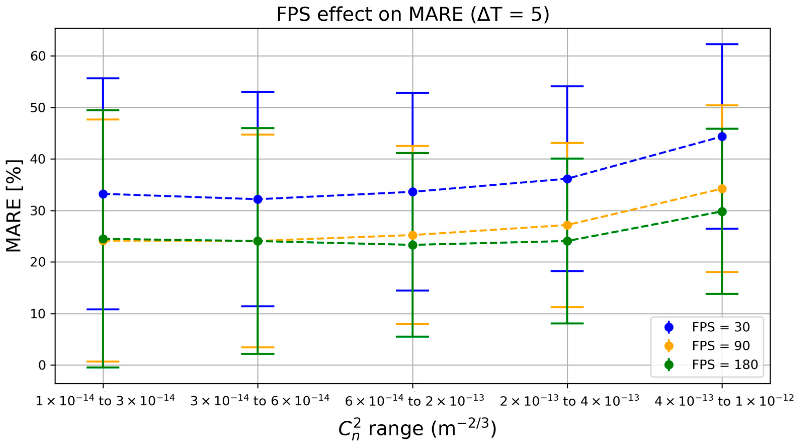
To evaluate the frame-based (CMOS) approach, we first assess its sensitivity to camera frame rate. Figure 2 illustrates the Mean Absolute Relative Error (MARE) of the CMOS model at three frame rates (30, 90, and 180 frames per second) across five turbulence strength ranges (from weak to strong turbulence, corresponding to path-integrated ${C_n}^2$ bins of approximately ${10}^{-14}$ to ${10}^{-12}$ ${\mathrm{m}}^{-2/3}$). As seen in Figure 2, the CMOS model’s accuracy improves consistently with increasing frame rate: the 30 FPS curve has the highest error in all turbulence regimes, 90 FPS is lower, and 180 FPS yields the lowest MARE. For example, in a moderate turbulence regime ($6\times {10}^{-14}–2\times {10}^{-13} {\mathrm{m}}^{-2/3}$), the average MARE drops from roughly 66% at 30 FPS to ~27% at 90 FPS and ~25% at 180 FPS. This trend aligns with expectations that a higher sampling rate captures rapid turbulence-induced distortions more effectively [11]. We also note that the overall error increases with turbulence strength, regardless of frame rate. Importantly, in the weak regime, the difference between 90 and 180 FPS was not significant, while in stronger regimes, the relative improvement with frame rate becomes more pronounced. This reflects the greater challenge of predicting stronger turbulence perturbations.

A one-way ANOVA [23] confirms that frame rate has a significant effect on error (F-test, p < 0.01). Tukey post hoc analysis [24] further reveals that the performance gains exhibit diminishing returns at high frame rates under weak turbulence. In the weakest turbulence range (${C_n}^2$ ~ 10⁻¹⁴–3 × 10⁻¹⁴), increasing frame rate from 90 FPS to 180 FPS produced a slight increase in mean MARE (24.15% vs. 24.50%), not an improvement. Statistical testing confirmed that this difference was not significant (p > 0.05). Thus, in low turbulence there is effectively no difference between 90 and 180 FPS, and both perform better than 30 FPS. By contrast, the jump from 30 FPS to 90 FPS is significant even in weak turbulence (MARE drops from 33.23% to 24.15% on average). Under strong turbulence (${C_n}^2$ ~ 4 × 10⁻¹³–10⁻¹²), the benefits of higher frame rates are pronounced: 180 FPS outperforms 90 FPS, which in turn outperforms 30 FPS, with all pairwise differences statistically significant (p < 0.01). For instance, at the highest turbulence level, the 30 FPS model’s MARE (mean 44.37%) is dramatically worse than the 90 FPS (34.23%) and 180 FPS (29.84%) models. These findings indicate that while increasing frame rate improves turbulence estimation accuracy overall, the improvement saturates beyond ~90 FPS in very weak turbulence conditions. In other words, under mild turbulence, the 90 FPS CMOS capture already provides most of the obtainable accuracy (180 FPS yields only a negligible extra benefit), whereas under intense turbulence, maximizing frame rate continues to pay dividends in reducing error.

4.2. Weak vs. Strong Turbulence Error Distributions (Frame-Rate Effect)

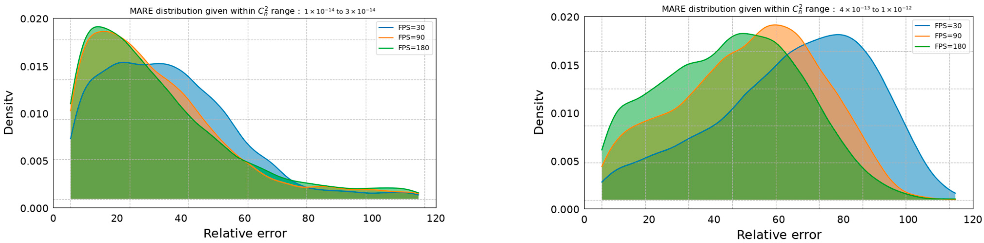
To further illustrate the above trends, Figure 3 compares the distribution of relative error (MARE) for the frame-based CMOS model across frame rates in two extreme regimes: weakest turbulence range (${{{1\times 10}^{-14} \le C}_n}^2<{3\times 10}^{-14}$) and strongest turbulence range (${{{4\times 10}^{-13} \le C}_n}^2<{1\times 10}^{-12}$). In the weakest turbulence case (Figure 3, left panel), the 90 FPS and 180 FPS error distributions substantially overlap, both concentrated at lower MARE values, whereas 30 FPS shows a broader distribution with a higher error median. The overlap between 90 FPS and 180 FPS and ANOVA/Tukey testing confirmed that the difference between them was not statistically significant (p > 0.05). By contrast, the 30 FPS distribution differed significantly from both 90 FPS and 180 FPS (p < 0.05), with a higher error median and broader spread. In contrast, under the strongest turbulence range (Figure 3, right panel), the error distributions separate cleanly: 30 FPS exhibits a heavy tail toward high relative errors, 90 FPS is markedly shifted to lower errors, and 180 FPS is further concentrated at the lowest error range. All frame rate pairs in strong turbulence differ significantly (p < 0.05), consistent with the ANOVA/Tukey results. In fact, the 90 FPS vs. 180 FPS gap widens in the strongest turbulence; the 180 FPS model has a lower mean error (29.8% vs. 34.2% at 90 FPS), though both share a similar standard deviation (~16%). These density plots underscore that under weak turbulence, capturing at 90 FPS is sufficient (additional frames do not appreciably improve accuracy), while under severe turbulence, maximizing frame rate yields proportionally large error reductions.

4.3. Comparison of Event-Only, Frame-Only, and Hybrid Models

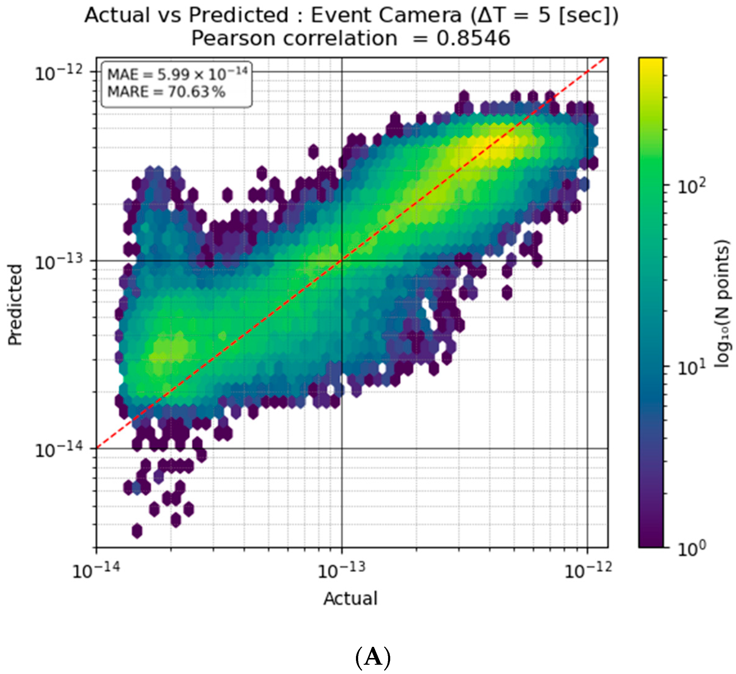
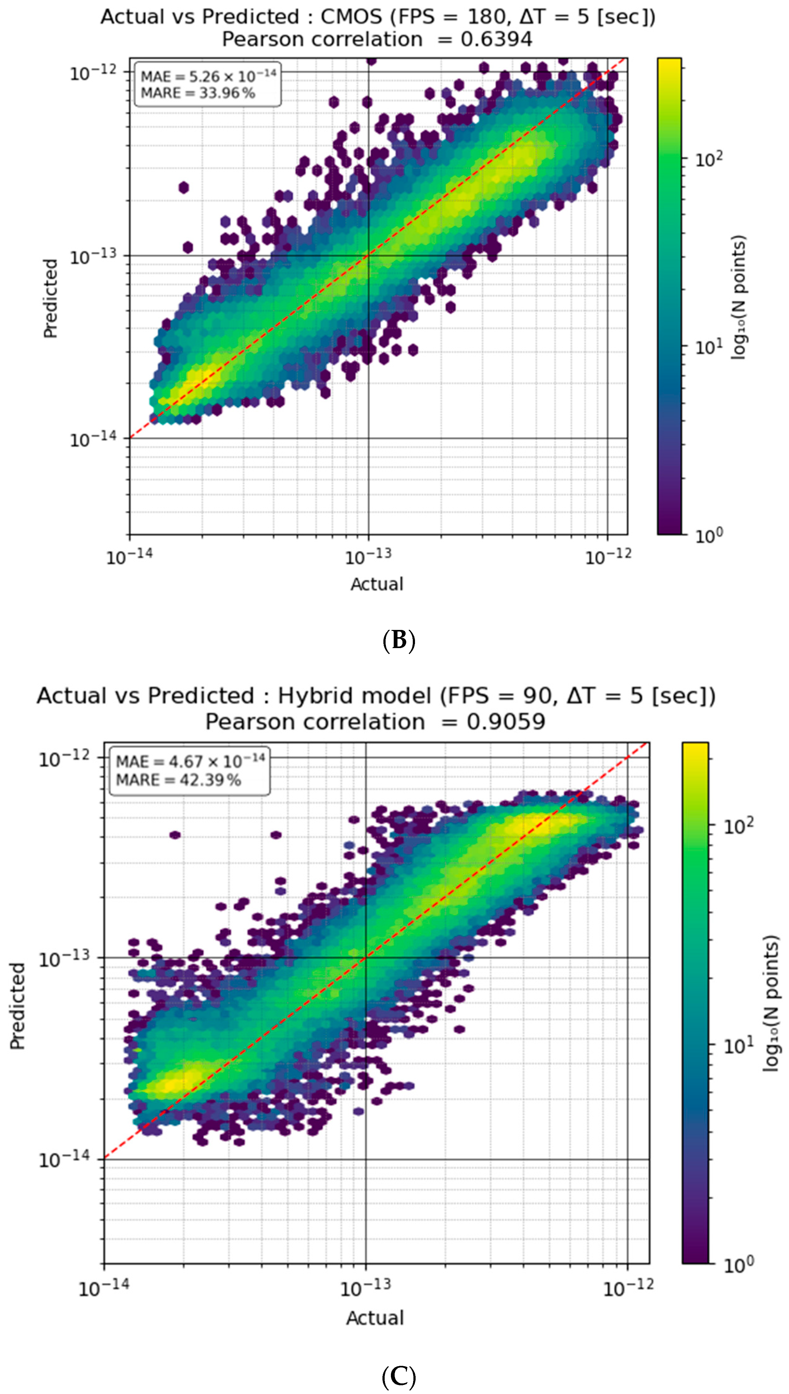
We next compare the turbulence estimation performance of three modeling approaches: an event-based model, a frame-based CMOS model, and a hybrid model fusing event and frame data. All models used the same 5 s observation window and high-contrast target imagery, with the CMOS-based model evaluated at its best frame rate (180 FPS) and the hybrid model using a 90 FPS frame input (plus the event stream). A hybrid configuration using 180 FPS CMOS was not included, as its improvement would be incremental and would not alter the main conclusion: that fusing events with a lower-frame-rate CMOS stream (90 FPS) can already surpass the performance of the 180 FPS CMOS-only model. Figure 4A–C presents scatter plots of the predicted ${C_n}^2$ versus the ground truth (BLS900 scintillometer measurements) for each model. Each figure also reports the Pearson correlation (r) between predictions and truth, along with the Mean Absolute Error (MAE) and MARE.

The scatter plot comparisons highlight distinct strengths of each approach. The event-based model (Figure 4A) produces predictions that are highly correlated with the true turbulence strength (r ≈ 0.85), suggesting that the fast temporal cues from the event sensor allow it to respond correctly to changes in turbulence intensity. However, its large MARE (~70%) indicates a tendency toward systematic bias or scale mismatch—likely underestimating ${C_n}^2$ in strong turbulence and/or overestimating in weak turbulence—resulting in high relative errors. This outcome is understandable, as pure event-based inference is a novel approach; events capture rapid motion (‘‘dancing’’ of the image) well [11], but they carry less direct information about absolute refractive index structure unless combined with intensity context. By contrast, the CMOS frame-only model (Figure 4B) yields much lower average relative error (~34%), indicating accurate magnitude estimates on average, especially in weaker turbulence regimes. This aligns with classical image-based turbulence estimation methods (e.g., the Zamek image-gradient variance method [5], which perform well in mild conditions. Yet, the frame-only model’s correlation r ≈ 0.64 is significantly lower; it struggles to correctly rank or synchronize with rapid turbulence fluctuations. Visually, the scatter for the CMOS model shows a moderate vertical spread across the turbulence range, consistent with its lower correlation relative to the event-based model. This suggests that the frame-based approach has difficulty capturing the full dynamic range of turbulence when using even high-speed (180 FPS) video, likely due to motion blur and limited temporal resolution within the 5 s window.

Finally, the hybrid (event + frame) model (Figure 4C) achieves the best of both worlds: it has a very high correlation (r ≈ 0.91) like the event-only model, and it maintains relatively low error magnitude (MARE ~42%) closer to the frame-only model. In fact, the hybrid’s correlation is the highest of all models, indicating it consistently tracks turbulence strength changes across the entire range. Its error distribution suggests improved performance, particularly at the higher turbulence end—the hybrid model can predict strong turbulence values more accurately than the frame-only model. This is impressive considering the hybrid used only 90 FPS imagery (half the frame rate of the CMOS-only model) yet still outperformed the latter in terms of correlation and high-turbulence accuracy. The result demonstrates the value of sensor fusion in this context: by combining the rich temporal information from the event camera with the per-frame intensity information from the CMOS sensor, the hybrid model overcomes limitations of each individual sensor. This approach parallels recent findings in turbulence mitigation research, where integrating multiple sensing modalities (e.g., adding a high-speed sensor or a narrow-band auxiliary image) improved performance [8,11]. Our results provide the quantitative evidence that an event+frame hybrid inference can yield superior turbulence strength estimation, particularly in challenging high-variability conditions.

4.4. Performance Across Turbulence Regimes

To better understand each model’s domain of effectiveness, we examine their errors in weak (${{{1\times 10}^{-14}\le C}_n}^2<{6\times 10}^{-14}$), moderate (${{{6\times 10}^{-14}\le C}_n}^2<{2\times 10}^{-13}$), and strong (${{{2\times 10}^{-13} \le C}_n}^2<{1\times 10}^{-12}$) turbulence regimes separately. Note that in previous subsections, turbulence was divided into five ranges to examine fine-grained trends, whereas here we simplify into three broader regimes. This aggregation was chosen to improve clarity when comparing distributions across models, without over-segmenting the analysis.

Table 2. Summary of relative error (MARE, %) for event-only, CMOS-only (180 FPS), and hybrid (event + CMOS 90 FPS) models across turbulence regimes (ΔT = 5 s, high-contrast target). Values denote median/mean MARE. See Table A1 in Appendix A for full statistics, including standard deviations and additional FPS variants.

Turbulence Regime	Event (ΔT = 5)	CMOS (180 FPS)	Hybrid (90 FPS)
Weak	42.56/62.05	23.77/34.44	27.53/39.69
Moderate	25.05/31.67	21.64/24.53	21.07/26.74
Strong	24.68/26.67	30.39/29.97	17.77/19.63

summarizes the error statistics (median and MARE) for each model under representative ranges of ${C_n}^2$. In weak turbulence, CMOS at 180 FPS achieves the lowest error (median/mean MARE ≈ 23.8/34.4%), outperforming the event-only and hybrid models; the hybrid 90 FPS remains close but higher (27.5/39.7%). In moderate turbulence, the gap narrows (CMOS 180 FPS 21.6/24.5%; hybrid 90 FPS 21.1/26.7%), while in strong turbulence the hybrid model is clearly best (17.8/19.6%), followed by event-only (24.7/26.7%) and CMOS 180 FPS (30.4/30.0%).

Below, we highlight the key comparisons in each regime (using the scintillometer-based turbulence binning defined earlier):

• Weak turbulence: In mild conditions, the frame-based CMOS models outperform the event-based and hybrid models. The 90 FPS CMOS model achieves the lowest mean error (~33% MARE), with the 180 FPS CMOS slightly higher (~34% MARE). Their performance is statistically indistinguishable (p > 0.05). The event-only model, however, suffers from very large errors in weak turbulence (mean MARE ~62%, median ~42%). The hybrid model at 90 FPS, which fuses these event signals with frames, fares better than event-alone but still has a higher error (~39% mean MARE) than the pure frame models. Notably, a hybrid model with only 30 FPS input performs worst of all (mean ~75% MARE), indicating that under slow, small turbulence distortions, the addition of event data cannot compensate for extremely low frame rates. In essence, when turbulence is weak, conventional frame-based estimation is sufficient and most accurate—the extra information from events is largely unnecessary and may introduce noise.
• Moderate turbulence: In intermediate conditions, all methods perform more comparably, though some advantages emerge. The CMOS model still benefits from high frame rate—at 180 FPS it achieves ~24.5% mean MARE, which is slightly better than the hybrid 90 FPS model (~26.7% MARE) and clearly better than the event-only model (~31.7% MARE). The 90 FPS frame-only model is also quite strong (~26.9% mean MARE), essentially matching the hybrid. These results suggest that in moderate turbulence, a high-frame-rate conventional camera can nearly match the hybrid’s accuracy on average. Nonetheless, the hybrid (and event) models show an edge in capturing variability: for example, the hybrid 90 FPS has a slightly lower median error (~21% vs. ~25% for CMOS), hinting that it more consistently estimates turbulence without severe outliers. Meanwhile, the hybrid 30 FPS version sees its error drop to ~30% mean MARE—a substantial improvement over its ~75% in weak turbulence—now approaching the event-only performance. This indicates that the event-based data become increasingly useful as turbulence intensifies, elevating even a low-FPS hybrid to respectable accuracy in moderate conditions.
• Strong turbulence: Under severe turbulence, the hybrid and event-based approaches decisively outperform the frame-only approach. The hybrid model with 90 FPS frames attains a mean MARE of only ~19.6%—by far the lowest in this regime—with median error ~17.8%, indicating very robust performance even at the upper end of turbulence strength. The event-only model is the next best, ~26.7% mean MARE, outperforming all purely frame-based results. Meanwhile, the best CMOS-only model (180 FPS) has a mean MARE ~30.0%, and the gap widens further at lower frame rates (34.3% at 90 FPS; 44.4% at 30 FPS). In other words, the hybrid model (90 FPS + events) reduces error by ~35% relative to the high-speed CMOS-only model in strong turbulence, a remarkable gain achieved despite using half the frame rate. Even the hybrid with 30 FPS frames yields ~22% mean MARE, beating the 180 FPS CMOS camera by a significant margin. These statistics confirm that when turbulence is strong, the fusion of event-based information with images is dramatically more effective than relying on frame data alone. The event camera’s ability to capture rapid, high-frequency wavefront tilts and intensity scintillations provides the hybrid model with an insight that a finite-frame-rate imager lacks [11]. Thus, for high turbulence, the hybrid approach is not only preferable—it is necessary to achieve low error and high correlation with true ${C_n}^2$.

Overall, this regime-wise comparison demonstrates a clear pattern: the CMOS model excels in low turbulence, but hybrid (and to a lesser extent event-only) models excel as turbulence grows stronger. The crossover in performance occurs at moderate turbulence levels, beyond which the event-driven methods become superior. These observations align with physical expectations and prior findings that classical image-based techniques work well under mild distortions [5], whereas unconventional sensing (events, multi-sensor fusion) is beneficial under more extreme conditions [8,11].

4.5. Error Distributions by Model Type and Turbulence Level

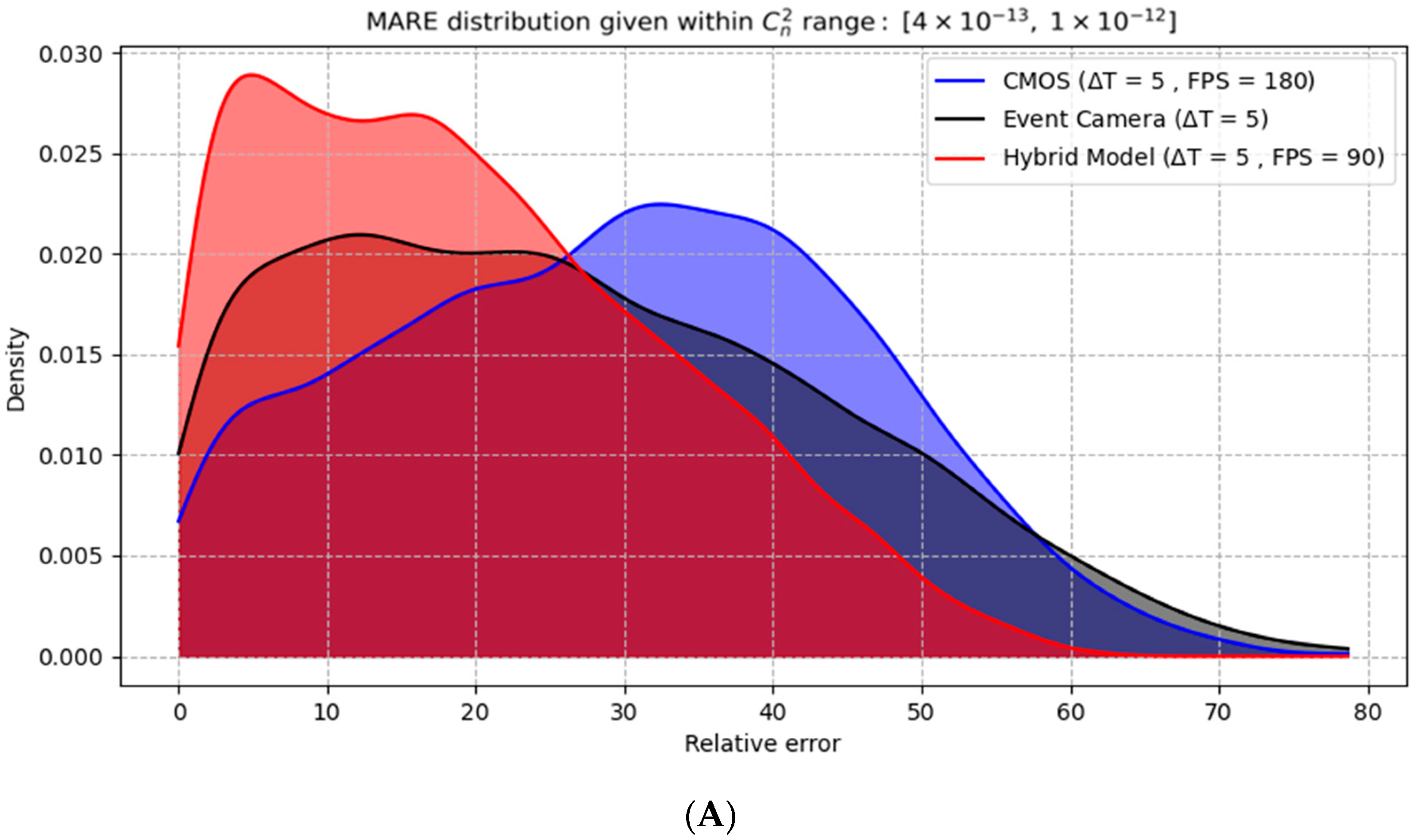
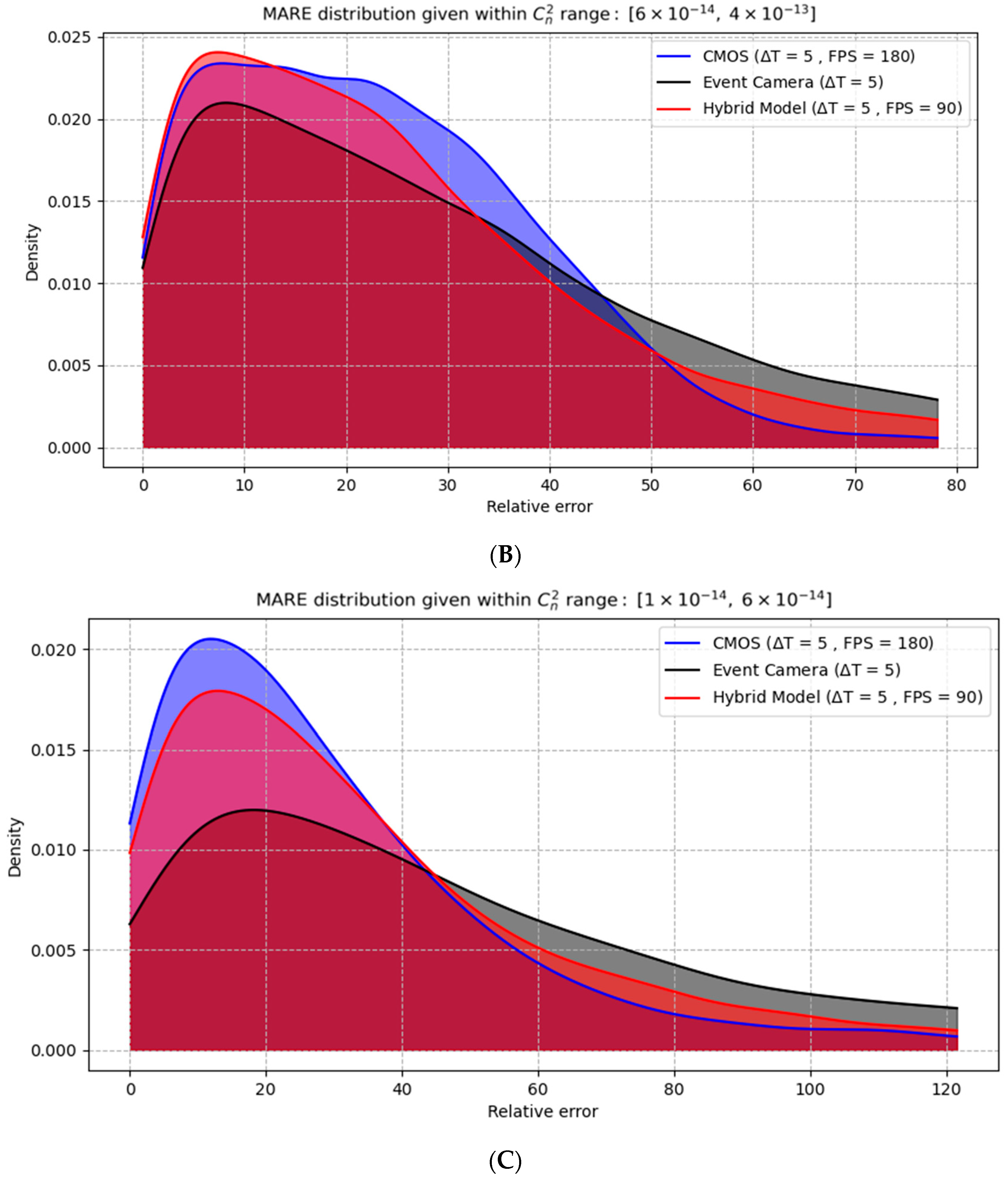
To visualize the distribution of errors for each model in different turbulence regimes, Figure 5A–C plots the probability density of MARE for the CMOS-only (180 FPS), event-only, and hybrid (90 FPS) models under strong, moderate, and weak turbulence. These density plots complement the numerical results above by revealing how consistently each model performs within a given regime.

Figure 5A–C underscores the regime-dependent performance of the three model types. In the strong turbulence plot (Figure 5A), the hybrid model not only has the lowest mean error but also the tightest distribution—a large fraction of its predictions are within 10–20% of ground truth, whereas the frame-based model frequently incurs 30–50% errors. The event model, while better than frame-only in strong turbulence, is slightly less consistent than the hybrid (its distribution’s tail is longer). Importantly, the hybrid model achieves better performance than either sensor alone, demonstrating that the event and frame modalities provide complementary information. Their combination yields improved results that cannot be achieved by either camera independently. In the moderate turbulence plot (Figure 5B), the methods converge; all yield a high peak at low errors, indicating that moderate distortions are tractable by any method given sufficient data (frames or events). Still, one can discern a minor advantage for the hybrid model (red), which maintains the highest density at the very lowest error values, reflecting its ability to capitalize on both modalities. Finally, in the weak turbulence plot (Figure 5C), the frame-only approach is clearly superior. The hybrid and event model distributions shift towards larger errors, likely due to the paucity of meaningful event data when turbulence-induced motion is tiny. The event camera in that scenario may fire mostly noise events, adding little useful signal and even degrading the hybrid model’s estimates. These distributional findings corroborate our earlier analysis: the hybrid approach is most beneficial in the high-turbulence regime, while in low-turbulence scenarios, a standard high-frame-rate camera already achieves optimal performance.

5. Discussion

5.1. Sensor-Specific Insights

Our comparative results show that the optimal sensor modality for turbulence strength estimation depends on the turbulence regime. In weak turbulence, the CMOS frame-based approach yielded lower error and more stable estimates of the refractive index structure constant (${C_n}^2$) than the event-based approach. For example, at low ${C_n}^2$, the frame camera (even at moderate frame rates) produced accurate turbulence estimates (see Figure 5C), whereas the event-based model exhibited a higher error floor. This is likely because in mild turbulence, the image distortions evolve slowly and subtly, triggering few events—the event camera’s output becomes sparse and noisy, hurting its accuracy. In contrast, the frame camera captures small distortion effects by integrating intensity changes over each frame. This aligns with traditional gradient-based turbulence metrics on conventional cameras: for instance, Zamek and Yitzhaky (2006) showed that the variance of image gradients in normal video frames correlates with ${C_n}^2$ [5]. Such frame-based methods work well when turbulence-induced changes are small and quasi-static, as in our weak-turbulence cases. Thus, each sensor excels in the regime matching its design (steady vs. fast distortion), and this dichotomy is supported by prior studies.

Under strong turbulence (large, fast index fluctuations), we observed the opposite: the event-based sensor captured rapid fluctuations better, achieving a higher correlation with the ground-truth ${C_n}^2$ time series than the frame-only sensor. Because an event camera reports brightness changes with microsecond-level latency [10], it can detect fast transient distortions (“image dancing” and blurring) that occur between the discrete frames of a CMOS camera. Indeed, event cameras offer very high temporal resolution (on the order of microseconds) and minimal motion blur [10], making them well-suited to record turbulence variations that a limited-FPS system might miss. In our experiments, the event stream responded immediately to sudden optical aberrations in strong turbulence, producing a turbulence-strength signal that tracked true fluctuations closely in time. However, the event-based estimates also showed higher variance and bias in strong turbulence, reflecting the difficulty of converting a flood of asynchronous events into a precise ${C_n}^2$ value. In summary, CMOS frame sensors excel in stable, weak turbulence (providing robust averaged metrics), whereas event sensors excel at capturing fast dynamics in strong turbulence (providing responsiveness at the cost of higher noise). This dichotomy is supported by prior knowledge: conventional video techniques handle slowly varying distortions well [5], and event cameras’ high-speed response adds value under rapid turbulence [10].

5.2. Frame Rate Tradeoffs

Another key finding is the influence of the CMOS camera’s frame rate on estimation accuracy. Increasing the frame rate substantially improved the ${C_n}^2$ estimation up to a certain point, beyond which returns diminish. Specifically, raising the frame rate from 30 FPS to 90 FPS yielded a notable drop in error for all turbulence strengths (capturing more temporal detail of the distortion). However, beyond ~90 FPS, the benefit plateaued for weak turbulence—at 180 FPS, there was minimal further error reduction (see Figure 2), suggesting that ~90 Hz sampling suffices to capture the relevant slow distortion dynamics. Additional frames mostly introduced redundant data and noise in that regime. In contrast, under strong turbulence, we observed continued gains from 90 FPS to 180 FPS, indicating that higher frame rates can still capture additional fast turbulence fluctuations. The error in strong turbulence kept decreasing up to our maximum tested rate, implying that even at 180 Hz, the camera was not fully sampling the rapid intensity variations. In practical terms, if only mild turbulence is expected, extremely high frame rates (>100 FPS) may not be necessary—a moderate frame rate may be cost-effective. But if severe turbulence is possible, a high-speed camera will markedly improve performance. This insight parallels the intuition in adaptive optics that the sampling frequency should match the turbulence variation rate. Notably, the event camera’s advantage in strong turbulence can be viewed similarly: its effective “frame rate” is in the kilohertz range [8], far beyond what traditional cameras can achieve. Thus, for weak turbulence, excessive frame rate offers diminishing returns, whereas for strong turbulence, a very high frame rate (or an event sensor) is justified.

5.3. Hybrid Inference Feasibility

Crucially, hybrid models (combining frame and event inputs) consistently outperformed the single-sensor models, especially in moderate-to-strong turbulence. Even a simple fusion of CMOS and event features produced a significant error reduction. In other words, the frame and event modalities capture different aspects of the turbulence (smooth vs. rapid changes), and fusing them yields a more complete picture of ${C_n}^2$ variations. In the strong turbulence regime, the hybrid model combining 90 FPS CMOS with events reduced mean error by ~35% compared to the CMOS-only model at 180 FPS (19.6% vs. 30.0 MARE, see

Table A1. Mean Absolute Relative Error (MARE, %) for all model variants across turbulence regimes using a 5 s integration window and high-contrast target. Values are reported as median/mean/standard deviation for CMOS (30/90/180 FPS), Event-only, and Hybrid (Event + CMOS at 30/90 FPS). These data underpin the condensed main-text Table 2 and the distribution plots.

Turbulence Regime	Metric	CMOS 30 FPS	CMOS 90 FPS	CMOS 180 FPS	Event (ΔT = 5)	Hybrid 30 FPS	Hybrid 90 FPS
Weak	Median	31.13	24.31	23.77	42.56	61.16	27.53
	Mean	35.85	33.18	34.44	62.05	75.51	39.69
	STD	30.54	35.62	37.66	59.37	62.60	41.05
Moderate	Median	43.42	25.44	21.64	25.05	23.21	21.07
	Mean	65.80	26.92	24.53	31.67	30.05	26.74
	STD	62.14	19.09	19.87	27.50	28.14	24.39
Strong	Median	46.73	35.78	30.39	24.68	20.36	17.77
	Mean	44.44	34.32	29.97	26.67	22.13	19.63
	STD	17.87	16.18	16.02	17.28	14.73	13.39

). This improvement underscores that the two sensors provide complementary information. Our results show that even basic data fusion can harness this complementarity, yielding more accurate and robust turbulence estimates than either sensor alone. In fact, the hybrid approach achieved the lowest estimation error under every turbulence condition in our tests.

It should be noted that the hybrid model was intentionally designed as a late-fusion approach, in which the CMOS-based turbulence estimate is appended as a scalar feature rather than jointly modeled with the event data; the implications of this design choice are discussed in Section 5.4.

This is in line with early experiments that combined event cameras with frame cameras. Boehrer et al. [8,25] found that using an event camera alongside a conventional camera led to sharper, more stable imagery through turbulence. In their case, the fused output retained fine detail better than any single-source image, demonstrating the value of even straightforward fusion. Similarly, our hybrid model leverages the event camera’s fast responsiveness plus the frame camera’s reliability, achieving better performance than either alone. Notably, Liu et al. (2025) have also leveraged event data in turbulence compensation: their EvTurb framework uses high-speed events to remove blur and tilt distortions from turbulent images, outperforming frame-only approaches [11]. All these findings support that event + frame fusion is not only feasible but advantageous for atmospheric turbulence applications. Our simple hybrid approach achieved substantial gains, suggesting that more advanced fusion (e.g., learned neural networks or adaptive filters) could further enhance performance in future work.

5.4. Limitations

There are several limitations to this study.

First, the proposed hybrid approach relies on late fusion, treating the CMOS-based turbulence estimate as an auxiliary input rather than performing joint spatiotemporal modeling of frame and event data. As a result, potential cross-modal interactions at the feature or signal level are not explicitly exploited. While this design was chosen deliberately to preserve interpretability and feasibility, it may limit performance gains compared to more tightly coupled or end-to-end fusion strategies, particularly under rapidly changing or highly non-stationary turbulence conditions.

Second, our experiments used a static, high-contrast target and did not include moving objects or complex backgrounds. This controlled setup ensured that all observed image motion was due to turbulence, but it does not test scenarios where scene motion and turbulence coexist. In real-world settings (e.g., surveillance or driving), separating turbulence-induced motion from object motion is challenging, and turbulence-induced image shifts can be mistaken for actual object movement. Similarly, since we tested primarily on an artificial resolution chart, the generalizability to natural scenes with diverse textures and spatial frequency content remains uncertain.

Nevertheless, prior work suggests that the qualitative advantages of event-based sensing are not limited to artificial targets. For example, Polnau and Vorontsov [16] demonstrated that neuromorphic event cameras can successfully characterize atmospheric turbulence when imaging real urban structures, such as buildings, indicating that the underlying turbulence signatures captured by event statistics extend beyond simple high-contrast patterns. While absolute performance levels may vary with scene texture and spatial frequency content, we expect the relative trends observed in this study—namely, the complementary behavior of frame-based and event-based sensing—to generalize to a broad class of natural scenes.

Third, our algorithms prioritized simplicity in feature extraction and fusion. We used basic statistical features and a straightforward fusion strategy to enable transparent comparison between sensing modalities. While effective, this approach is unlikely to be optimal. More sophisticated machine-learning or physics-informed models could potentially better suppress noise, adapt to varying turbulence regimes, or exploit richer cross-feature interactions.

In addition, event-sensor parameters were not extensively tuned for weak turbulence conditions, where thresholding effects may reduce sensitivity.

Finally, the experimental conclusions were derived from a specific propagation geometry, with a fixed path length, aperture size, and near-ground horizontal line of sight.

Variations in these parameters—such as longer propagation distances, larger apertures (introducing aperture-averaging effects), or elevated paths with different turbulence profiles—may influence absolute estimation error for both sensing modalities. However, because both frame-based and event-based sensors are governed by the same underlying wave-propagation physics, we expect the relative performance trends and comparative conclusions reported here to remain qualitatively valid across a wide range of practical configurations.

In addition, variations in illuminance due to changing weather conditions (e.g., cloud cover or solar angle) may affect image contrast and signal quality, particularly for frame-based cameras. Event cameras, which respond to relative brightness changes rather than absolute intensity, are inherently more robust to slow global illumination variations, although abrupt localized illumination transients may still generate spurious events. These factors should be considered when deploying the proposed methods under varying environmental conditions.

5.5. Implications for Deployment

Our findings have practical implications for systems that deal with atmospheric turbulence. In free-space optical communication, a hybrid sensor could provide real-time monitoring of turbulence strength along a laser link, enabling adaptive modulation or power control. For example, it could be integrated into an optical transceiver station to continuously gauge channel quality. In adaptive optics for imaging, a frame+event sensor could assist in conditions where traditional adaptive optics struggles—such as horizontal imaging or extended scenes where wavefront correction is non-uniform [25]. The hybrid sensor could feed an AO system with both steady turbulence estimates and alerts to rapid changes, improving correction for wide-field or ground-level imaging. In atmospheric monitoring, camera-based ${C_n}^2$ sensors are a low-cost alternative to scintillometers (especially as event cameras become more accessible); our results suggest that adding an event-based channel would make such sensors more sensitive to fast turbulence fluctuations, improving measurements for meteorology or aviation safety. Finally, in astronomy, an event-enhanced seeing monitor (e.g., a differential image motion monitor) could track high-frequency seeing fluctuations better than a conventional camera, informing observers or automated systems to adjust focus, exposure, or select lucky frames. Across all these domains, the enhanced accuracy and responsiveness of a hybrid sensor could translate into more resilient and higher-quality optical systems operating under turbulent atmospheric conditions in practice [5,8,10,11].

6. Conclusions

This study provides a comprehensive comparison of frame-based (CMOS camera) and event-based optical turbulence strength estimation, and demonstrates the benefits of a hybrid approach combining both. Our results show that conventional frame-based models achieve the highest accuracy under weak turbulence conditions. This is consistent with prior passive imaging methods (e.g., the gradient-based estimator of Zamek & Yitzhaky [5]), which perform reliably when distortion is minimal. However, as turbulence intensifies, frame-based model performance deteriorates markedly. We observed a decline in measurement linearity and increased error at stronger turbulence levels, reflecting known limitations of CMOS-based techniques under severe optical distortion [14].

In contrast, the event-based approach excelled in the strong-turbulence regime. Event cameras inherently capture rapid brightness changes with very low latency, offering a high dynamic range and virtually no motion blur [10,26]. These characteristics allow the event-based method to effectively track fast, turbulence-induced intensity fluctuations even when atmospheric distortions are pronounced. Indeed, event-based sensors showed robust estimation accuracy in high turbulence conditions in our experiments. Conversely, under weak turbulence, the event-driven method exhibited relatively large errors. This is likely due to the sparse event output (fewer brightness changes to detect) when turbulence is mild, which makes the estimation more susceptible to sensor noise and quantization error. In low-disturbance conditions, frame-based imagery provides a denser information stream, whereas the event sensor’s advantages are less leveraged.

By fusing these complementary sensing modalities, the proposed hybrid models achieved the best overall performance across a wide range of turbulence strengths. The hybrid approach (combining CMOS frames and asynchronous event data) yielded the highest accuracy and correlation with ground-truth turbulence measurements in moderate-to-strong turbulence, outperforming either sensor alone. Notably, a hybrid model using a 90 FPS CMOS camera together with an event sensor significantly outperformed a standalone 180 FPS frame-based system under strong turbulence, reducing the estimation error by approximately 35%. This substantial improvement underscores the efficacy of sensor fusion: the frame-based component provides reliable baseline measurements in stable moments, while the event-based component contributes timely detection of rapid turbulence fluctuations. The result is a more resilient estimator that maintains accuracy even as turbulence conditions worsen.

Overall, our findings confirm that CMOS frame-based and event-based sensors have complementary strengths for optical turbulence sensing. Frame-based methods are well-suited for capturing fine details in steady or weak turbulence, whereas event cameras offer superior responsiveness in rapidly changing, high-turbulence scenarios. The fusion of both sources thus provides a robust, adaptive solution that can handle the full spectrum of turbulence regimes. In conclusion, harnessing this complementary behavior via hybrid sensing approaches has great potential to improve real-time optical turbulence monitoring. Such improvements are particularly relevant for high-precision applications that must contend with atmospheric distortion. For instance, accurate turbulence estimates are essential for adaptive optics systems in astronomy to correct wavefront errors, and for free-space optical communication links to mitigate signal fading [27]. The demonstrated success of the frame-event hybrid model suggests a promising path forward for enhancing the reliability of turbulence strength estimation, ultimately supporting more resilient optical systems in challenging atmospheric environments.

7. Future Work

The hybrid approach presented in this study provides a proof of concept for integrating event-based and frame-based sensors in turbulence strength estimation. Several promising directions can extend this work.

First, deep learning architectures offer the potential to fuse spatiotemporal information more effectively than handcrafted features. Convolutional neural networks and transformer-based models could jointly encode asynchronous events and video frames, capturing turbulence effects across scales. Prior work demonstrates the feasibility of such strategies: Qu et al. [28] applied a CycleGAN to mitigate turbulence in optical links, and Zhang et al. [29] introduced a Turbulence Mitigation Transformer that improved performance on distorted imagery. Liu et al. [11] further showed that event data enable state-of-the-art turbulence removal. In addition, Mizrahi, Laufer, and Zuckerman [18] proposed a CNN–DGCNN architecture for real-world spatial synchronization of event and CMOS cameras, highlighting the promise of joint inference within a unified network. These advances suggest that tailored hybrid networks could outperform the simple scalar fusion used here.

In parallel, feature engineering could enrich the representation of turbulence effects. Gradient matrices from frame sequences, optical flow, or motion vectors, and spatiotemporal “event point clouds” can capture complementary information about image dancing, blurring, and scintillation. Incorporating such features, either directly or within a learned framework, could improve sensitivity across turbulence regimes [30].

A critical step toward application is real-time deployment. For adaptive optics and free-space optical communication, estimates must be delivered with minimal latency. Implementation on FPGA or GPU platforms could enable live inference, leveraging parallel processing of high-throughput event streams [31]. Recent studies demonstrate the feasibility of real-time turbulence compensation using neural networks, suggesting that streamlined hybrid pipelines could achieve similar performance [30,32].

Further experimental validation is also needed. While the current study focused on a controlled 300 m path and artificial targets, field trials should include kilometer-scale links, varied altitudes, and natural scenes such as trees, buildings, or astronomical sources. Such tests would probe robustness across realistic environments and turbulence profiles. The availability of datasets like TurbEvent [11] also provides an opportunity for benchmarking and broader comparisons.

Another avenue is uncertainty-aware modeling, where predictions are accompanied by confidence measures. Bayesian neural networks or dropout-based sampling, as explored by Yasarla and Patel [33] for turbulence-degraded images, could allow the hybrid model to output both estimates and reliability scores. This would inform downstream decisions in adaptive optics or communications systems, enabling dynamic adjustment of correction strategies.

Finally, practical engineering challenges must be addressed. Event threshold settings must balance sensitivity with noise, and optimal tuning may vary with turbulence regime (e.g., [34]). Accurate time synchronization between event and frame sensors is essential, as even millisecond misalignment can degrade fusion. Cross-sensor calibration for spatial alignment must also be robust to ensure consistent feature mapping. Developing adaptive calibration and synchronization methods will be crucial for robust field deployment [31].

In sum, the present work establishes feasibility but also reveals clear opportunities for advancement. By combining deep learning fusion, enriched features, real-time hardware implementations, extensive field validation, and uncertainty-aware modeling, future studies can evolve the hybrid approach from a proof of concept to a robust tool for turbulence sensing. Such systems could significantly improve atmospheric correction in astronomy, strengthen free-space optical links, and enhance environmental monitoring by exploiting the complementary strengths of event-driven and frame-based vision.

References

1. Hegde, R.; Anand, N.; Satheesh, S.K.; Moorthy, K.K. Modeling the atmospheric refractive index structure parameter using macrometeorological observations. Appl. Opt. 2024, 63, E10–E17. [Google Scholar] [CrossRef]
2. Tatarski, V.I. Wave Propagation in a Turbulent Medium; Courier Dover Publications: Garden City, NY, USA, 2016. [Google Scholar]
3. Roddier, F. Adaptive Optics in Astronomy; Cambridge University Press: Cambridge, UK, 1999. [Google Scholar]
4. Hill, R.J. Algorithms for obtaining atmospheric surface-layer fluxes from scintillation measurements. J. Atmos. Ocean. Technol. 1997, 14, 456–467. [Google Scholar] [CrossRef]
5. Zamek, S.; Yitzhaky, Y. Turbulence strength estimation from an arbitrary set of atmospherically degraded images. J. Opt. Soc. Am. A 2006, 23, 3106–3113. [Google Scholar] [CrossRef]
6. Potvin, G. Relationship between turbulent image variance and average image gradient. J. Opt. Soc. Am. A 2024, 41, B32–B39. [Google Scholar] [CrossRef] [PubMed]
7. Roggemann, M.C.; Welsh, B.M. Imaging Through Turbulence; CRC Press: Boca Raton, FL, USA, 2018. [Google Scholar]
8. Boehrer, N.; Nieuwenhuizen, R.; Dijk, J. Using event cameras for imaging through atmospheric turbulence. In Proceedings of the COAT-2019—Workshop (Communications and Observations Through Atmospheric Turbulence: Characterization and Mitigation), Châtillon, France, 2–3 December 2019. [Google Scholar]
9. Rebecq, H.; Ranftl, R.; Koltun, V.; Scaramuzza, D. High speed and high dynamic range video with an event camera. IEEE Trans. Pattern Anal. Mach. Intell. 2019, 43, 1964–1980. [Google Scholar] [CrossRef]
10. Gallego, G.; Delbrück, T.; Orchard, G.; Bartolozzi, C.; Taba, B.; Censi, A.; Leutenegger, S.; Davison, A.J.; Conradt, J.; Daniilidis, K.; et al. Event-based vision: A survey. IEEE Trans. Pattern Anal. Mach. Intell. 2020, 44, 154–180. [Google Scholar] [CrossRef] [PubMed]
11. Liu, Y.; Teng, M.; Xia, Y.; Duan, P.; Shi, B. EvTurb: Event Camera Guided Turbulence Removal. arXiv 2025, arXiv:2508.10582. [Google Scholar] [CrossRef]
12. Rebecq, H.; Ranftl, R.; Koltun, V.; Scaramuzza, D. Events-to-video: Bringing modern computer vision to event cameras. In Proceedings of the IEEE/CVF Conference on Computer Vision and Pattern Recognition, Long Beach, CA, USA, 15–20 June 2019; pp. 3857–3866. [Google Scholar]
13. Atrey, P.K.; Hossain, M.A.; El Saddik, A.; Kankanhalli, M.S. Multimodal fusion for multimedia analysis: A survey. Multimed. Syst. 2010, 16, 345–379. [Google Scholar] [CrossRef]
14. Saha, R.K.; Salcin, E.; Kim, J.; Smith, J.; Jayasuriya, S. Turbulence strength Cn2 estimation from video using physics-based deep learning. Opt. Express 2022, 30, 40854–40870. [Google Scholar] [CrossRef] [PubMed]
15. Mizrahi, D.; Brisk, D.; Mordechai, Y.; Maor, O. Event-Based Camera Modeling for Atmospheric Turbulence Prediction. Sensors 2025, 25, 7276. [Google Scholar] [CrossRef]
16. Polnau, E.; Vorontsov, M.A. Atmospheric turbulence characterization using a neuromorphic camera-based imaging sensor. J. Opt. 2021, 23, 125608. [Google Scholar] [CrossRef]
17. Chen, T.; Guestrin, C. Xgboost: A scalable tree boosting system. In Proceedings of the 22nd ACM SIGKDD International Conference on Knowledge Discovery and Data Mining, San Francisco, CA, USA, 13–17 August 2016; pp. 785–794. [Google Scholar]
18. Mizrahi, D.; Laufer, I.; Zuckerman, I. Real-World Spatial Synchronization of Event-CMOS Cameras through Deep Learning: A Novel CNN-DGCNN Approach. Sensors 2024, 24, 4050. [Google Scholar] [CrossRef]
19. Duan, H.; Guo, C.; Ou, Y. Fusing Events and Frames with Coordinate Attention Gated Recurrent Unit for Monocular Depth Estimation. Sensors 2024, 24, 7752. [Google Scholar] [CrossRef]
20. Apicella, A.; Isgrò, F.; Prevete, R. Don’t push the button! exploring data leakage risks in machine learning and transfer learning. Artif. Intell. Rev. 2025, 58, 339. [Google Scholar] [CrossRef]
21. Nikou, M.K.; Ehsani, M.R. Turbulence models application on CFD simulation of hydrodynamics, heat and mass transfer in a structured packing. Int. Commun. Heat Mass Transf. 2008, 35, 1211–1219. [Google Scholar] [CrossRef]
22. Azimi, H.; Shabanlou, S.; Kardar, S. Turbulent flow in the vicinity of side weirs in subcritical conditions. Math. Model. Comput. Simul. 2018, 10, 784–797. [Google Scholar] [CrossRef]
23. Edwards, A.W. RA Fischer, Statistical Methods for Research Workers, (1925). In Landmark Writings in Western Mathematics 1640–1940; Elsevier Science: Amsterdam, The Netherlands, 2005; pp. 856–870. [Google Scholar]
24. Tukey, J.W. Comparing Individual Means in the Analysis of Variance. Biometrics 1949, 5, 99–114. [Google Scholar] [CrossRef] [PubMed]
25. Boehrer, N.; Nieuwenhuizen, R.P.; Dijk, J. Turbulence mitigation in imagery including moving objects from a static event camera. Opt. Eng. 2021, 60, 053101. [Google Scholar] [CrossRef]
26. Chakravarthi, B.; Verma, A.A.; Daniilidis, K.; Fermuller, C.; Yang, Y. Recent event camera innovations: A survey. In Proceedings of the European Conference on Computer Vision, Milan, Italy, 29 September–4 October 2024; Springer Nature: Cham, Switzerland, 2024; pp. 342–376. [Google Scholar]
27. Bi, C.; Qing, C.; Wu, P.; Jin, X.; Liu, Q.; Qian, X.; Zhu, W.; Weng, N. Optical turbulence profile in marine environment with artificial neural network model. Remote Sens. 2022, 14, 2267. [Google Scholar] [CrossRef]
28. Qu, T.; Zhang, Y.; Wu, J.; Wu, Z. Vortex Beam Transmission Compensation in Atmospheric Turbulence Using CycleGAN. Photonics 2023, 10, 1182. [Google Scholar] [CrossRef]
29. Zhang, X.; Mao, Z.; Chimitt, N.; Chan, S.H. Imaging through the atmosphere using turbulence mitigation transformer. IEEE Trans. Comput. Imaging 2024, 10, 115–128. [Google Scholar] [CrossRef]
30. Hoffmire, M.A.; Hardie, R.C.; Rucci, M.A.; Van Hook, R.; Karch, B.K. Deep learning for anisoplanatic optical turbulence mitigation in long-range imaging. Opt. Eng. 2021, 60, 033103. [Google Scholar] [CrossRef]
31. Kryjak, T. Event-based vision on fpgas-a survey. In Proceedings of the 27th Euromicro Conference on Digital System Design (DSD), Paris, France, 28–30 August 2024; IEEE: Piscataway, NJ, USA, 2024; pp. 541–550. [Google Scholar]
32. Shankaranarayanan, H.; Yadav, S.S.; Adithya Krishna, A.; Vikram, P.; Mehendale, M. HOMI: Ultra-Fast EdgeAI platform for Event Cameras. arXiv 2025, arXiv:2508.12637. [Google Scholar]
33. Yasarla, R.; Patel, V.M. Learning to restore images degraded by atmospheric turbulence using uncertainty. In Proceedings of the 2021 IEEE International Conference on Image Processing (ICIP), Anchorage, AK, USA, 19–22 September 2021; IEEE: Piscataway, NJ, USA, 2021; pp. 1694–1698. [Google Scholar]
34. Wang, Z.; Ng, Y.; van Goor, P.; Mahony, R. Event camera calibration of per-pixel biased contrast threshold. arXiv 2020, arXiv:2012.09378. [Google Scholar] [CrossRef]
Figure 1. Schematic of the 300 m experimental path and co-located sensors at the Yavne, Israel. The Basler CMOS camera and Prophesee event camera were mounted together at the receiver station, aligned alongside the BLS900 scintillometer receiver to observe the target panel at the transmitter station. This multimodal configuration (frame-based and event-based cameras plus scintillometer) shares a common line-of-sight, enabling simultaneous capture of atmospheric turbulence effects in both conventional video frames and asynchronous event streams.
Atmosphere 17 00024 g001
Figure 2. Effect of frame rate on the CMOS model’s MARE (Mean Absolute Relative Error) across five turbulence strength ranges (log-scaled C n 2 bins) for a 5 s integration window. Higher frame rates yield consistently lower errors, though improvements saturate at the highest rates for weak turbulence. Error bars indicate ±1 std. of MARE; overlapping error bars between 90 FPS and 180 FPS in the weakest turbulence bin suggest their performance difference is not statistically significant.
Atmosphere 17 00024 g002
Figure 3. Kernel density plots of CMOS model MARE for 30 FPS, 90 FPS, and 180 FPS in weak vs. strong turbulence conditions. (Left): Weak turbulence (range 1)—90 FPS and 180 FPS distributions nearly overlap, indicating similar performance, whereas 30 FPS has a longer error tail. (Right): Strong turbulence (range 5)—distributions are clearly separated, with 180 FPS achieving the lowest errors, 90 FPS intermediate, and 30 FPS the highest errors.
Atmosphere 17 00024 g003
Figure 4. (A): Actual vs. predicted turbulence strength for the event-based XGBoost model (using only event camera data). Points are colored by density (hexbin log-density). The event-based model achieves a Pearson correlation of r ≈ 0.85, indicating it captures the overall trend of C n 2 variations well. However, its error magnitudes are relatively high: MAE ≈  5.99 ×   10 14   m 2 / 3 and MARE ≈ 70.6% (i.e., on average predictions deviate ~70% from true values). (B): Actual vs. predicted turbulence strength for the CMOS frame-based model at 180 FPS. This model shows a lower overall error (MAE ≈ 5.26 ×   10 14   m 2 / 3 , MARE ≈ 33.9%) than the event-only model, especially in the lower C n 2 range. However, the Pearson correlation is only r ≈ 0.64, substantially lower than the event-based approach. The scatter indicates that the frame-only predictions tend to under-correlate with true turbulence fluctuations, particularly under higher turbulence conditions (many points deviate from the y = x line). (C): Actual vs. predicted turbulence strength for the hybrid model (event + CMOS at 90 FPS). This hybrid approach achieves the highest correlation with ground truth (r ≈ 0.906), demonstrating excellent agreement in tracking turbulence variations. Its MAE (≈ 4.67 ×   10 14   m 2 / 3 ) is the lowest of the three models, and MARE (≈42.4%) is intermediate between the frame-only and event-only models. Notably, even with only 90 FPS image input, the hybrid model’s accuracy approaches that of a 180 FPS frame-only system, thanks to the complementary high-temporal-resolution event data.
Atmosphere 17 00024 g004aAtmosphere 17 00024 g004b
Figure 5. (A): Distribution of relative error (MARE) for the three models in strong turbulence ( 4 × 10 13 < C n 2 10 12 ). The hybrid model (red curve) produces a sharply peaked error distribution near low values (peak around 10–15% error) and a short tail, indicating that it rarely incurs large errors under strong turbulence. The event-based model (black) also skews toward low errors, though with a slightly broader tail than the hybrid. In contrast, the CMOS 180 FPS model (blue) exhibits a broader distribution centered at higher errors (~25–30%), with a longer tail extending toward 50–60% errors. This demonstrates the hybrid model’s superior reliability in high-turbulence conditions, effectively reducing large error outliers relative to the frame-only approach. (B): Distribution of relative error for moderate turbulence ( 6 × 10 14 < C n 2 4 × 10 13 ). Here, the three methods show more overlap. The CMOS 180 FPS (blue) and hybrid 90 FPS (red) error distributions are both tightly clustered at low errors (peaking ~10% and ~8% MARE, respectively). The hybrid’s curve is marginally to the left of the CMOS, reflecting a slightly lower median error, but their tails (extending to ~50–60%) are comparable. The event-only model (black) has an error distribution largely overlapping the others in this regime, though its density is a bit more spread out (indicating a few more instances of higher errors). Overall, in moderate turbulence, all three approaches achieve low errors most of the time, with only subtle differences—the hybrid retains a slight advantage in keeping errors concentrated at the lowest values. (C): Distribution of relative error for weak turbulence ( 10 14 < C n 2 6 × 10 14 ). Under weak conditions, the frame-based CMOS model (blue) clearly outperforms the others: its error distribution peaks at ~10–15% and has a relatively short tail (few instances exceed 60% error). The hybrid model (red) yields a broader distribution with a peak around ~15–20% and a tail extending beyond 80% MARE. The event-only model (black) performs worst, with a flatter distribution and a very long tail of high errors (including some instances over 100% relative error, meaning the prediction error can exceed the true value). These distributions confirm that when turbulence is minimal, purely frame-based estimation is both more accurate and more consistent than event-driven approaches, which struggle due to the low signal (few intensity changes) in the event stream.
Atmosphere 17 00024 g005aAtmosphere 17 00024 g005b