SD-WACCM-X Study of Nonmigrating Tidal Responses to the 2019 Antarctic Minor SSW

Abstract

The 2019 Antarctic sudden stratospheric warming (SSW) is well captured by the specified dynamics Whole Atmosphere Community Climate Model with thermosphere and ionosphere eXtension (SD-WACCM-X). This SSW is dominated by a strong quasi-stationary planetary wave with zonal wavenumber 1 (SPW1) activity, and nonmigrating tides show great variations. The nonlinear interactions between SPW1 and diurnal, semidiurnal and terdiurnal migrating tides triggered by this SSW also have significant impacts on the variabilities of corresponding nonmigrating tides. This is clearly proven by the fact that the variations of the secondary nonmigrating tides, generated by the nonlinear interaction, show higher correlation during this SSW than those during the non-SSW period. Meanwhile, the SPW1 dominates the nonlinear interactions with diurnal, semidiurnal and terdiurnal migrating tides, and the corresponding secondary nonmigrating tides show concurrent increases with SPW1. In the ionosphere, the nonmigrating tidal oscillations exhibit consistent temporal variabilities with those shown in the neutral atmosphere, which demonstrates the neutral–ion coupling through nonmigrating tides and that nonmigrating tides are significant sources for the short-term ionospheric variability during this SSW event. Specifically, the enhancement of the ionospheric longitudinal wavenumber 4 structure coincides with the increase of the eastward-propagating diurnal tide with zonal wavenumber 3 (DE3), semidiurnal tide with zonal wavenumber 2 (SE2) and terdiurnal tide with zonal wavenumber 1 (TE1). Also, DE3 dominates the influence of nonmigrating tides on the ionospheric longitudinal wavenumber 4 structure during this SSW.

1. Introduction

Sudden stratospheric warming (SSW) is a kind of common dramatic large-scale atmospheric phenomenon occurring in the polar stratospheric regions in winter. During SSWs, the temperature increases rapidly within a short time, and the zonal mean zonal wind weakens or even reverses direction in the stratosphere [1]. According to different, changing types of temperature gradient and zonal mean zonal wind, the World Meteorological Organization (WMO) has defined the classifications of SSW. At 10 hPa and latitude 60 degrees (whether in the northern hemisphere (NH) or southern hemisphere (SH)), a major SSW is defined with temperature increasing and zonal mean zonal wind reversing, while a minor SSW shows an increase in temperature and deceleration of zonal mean zonal wind [2,3]. It is widely accepted that quasi-stationary planetary waves (SPWs) propagating from the lower atmosphere and their interaction with mean flow patterns play a crucial role and lead to SSW [1,4]. In the polar region of the NH, SSW occurs more frequently, a little more frequently than every two winters. However, due not only to smaller SPW amplitudes but also to a stronger and more persistent stratospheric polar vortex, the occurring frequencies of SSW are much lower in the winter polar region of the SH [5]. Of all the Antarctic SSWs that have occurred, one occurred in 2019 [6,7].

SSW also has great impacts on the states of the mesosphere, lower thermosphere and ionosphere, although it mainly occurs in the stratosphere, which has been demonstrated in both observations and simulations [8,9,10,11]. Baldwin systematically describes the historical background, dynamical processes, modeling, chemistry and effects on the atmosphere of SSW [12]. In Section 8 of Baldwin’s review article, it briefly reviews the major impacts of SSWs on the upper stratosphere–mesosphere, thermosphere and ionosphere, including the effects of SSW on atmospheric tides. Atmospheric tides are a kind of global-scale atmospheric oscillations which can propagate to the upper atmosphere from the lower atmosphere and propagate eastward or westward with zonal wavenumber s (s = 1,2,3…) in the horizontal propagation direction. Their main periods are diurnal, semidiurnal and terdiurnal corresponding to solar days [13,14]. Thus, according to different periods, horizontal propagating directions and zonal wavenumbers, atmospheric tides are named Des, DWs, Ses, SWs, Tes, TWs, and so on. The D, S and T represent diurnal, semidiurnal and terdiurnal, respectively; the E and W indicate the horizontal propagating direction is eastward and westward, respectively; zonal wavenumber is represented by s. If the tide remains stationary in the horizontal propagation direction, there is no second term (E/W). During SSWs, the upward-propagating atmospheric tides show dramatic variabilities in the neutral atmosphere, and these tides also have significant impacts on the short-term ionospheric variabilities [9,15,16,17]. To date, the direct propagation of changing tides and vertical drift modulated through the E-region dynamo mechanism by the tides are thought to be triggers of ionospheric responses to SSW [17,18,19,20,21,22]. Thus, considering the important role of tides during SSWs, tidal variations and influences during different SSWs have been a hot topic.

Pedatella and Forbes revealed semidiurnal nonmigrating and migrating perturbations in the Equatorial Ionization Anomaly (EIA) region by using ionospheric observations during the 2009 SSW, and they indicated that these ionospheric perturbations are associated with a tidal dynamo [23]. Pedatella and Liu simulated different kinds of SSW events using TIME-GCM to investigate tidal variabilities in the neutral atmosphere and their influences on the ionosphere of low-latitude regions during SSWs [16]. They found that SW2 shows distinct increases during SSWs, and its nonlinear interactions with zonal wavenumber 1 (SPW1), can lead to significant increases of SW1. Meanwhile, the enhanced SW1 has been found to make contributions to the ionospheric variabilities in low-latitude regions during SSWs. Yue et al. found that there was a global response in the ionosphere during the 2009 SSW based on ionospheric observations, and they thought that the mid- and high-latitude ionospheric variations might be associated with the direct propagations of tides [22]. Yasyukevich studied ionospheric variations of the F2 region peak electron density (NmF2) during 12 different Arctic SSWs over 2006–2013, and the results agreed that tides play a significant role in SSW-related ionospheric variations [17]. Fuller-Rowell et al. explored the impacts of SSW on thermosphere dynamics and electrodynamics by using a whole atmosphere model [24]. They showed tidal variations and found that SSW can induce the increases of TW3. A long-term weakening of DW1 and TW3 and a short-term enhancement of SW2 in the ionosphere during the 2009 SSW have been reported by Jin et al. [25]. Eswaraiah et al. analyzed the effects of the 2002 major and 2010 minor Antarctic SSWs on mesospheric tides based on observations, and they discussed why tidal enhancements occurred with a delay after the SSW [26]. Guharay and Batista investigated tidal responses to the 2002 major SSW in the middle atmosphere based on observations [27]. A distinct decrease of DW1 and obvious increases of SE1, SW1, SW2 and SW4 were visible during this SSW, and they also found the responses of DW1 and SW1 were mostly active in this major SSW. Teng et al. studied tidal variations during three Antarctic SSWs and found that TW3 showed unexpected decreases in the neutral atmosphere and ionosphere based on simulations [28].

Limited by the frequency of SSW occurrence in the SH, there are only a limited number of recorded Antarctic SSWs [6,26,29,30]. Thus, Antarctic SSW-related studies on tidal variations and influences are relatively rare compared to those tidal studies during Arctic SSWs. The 2019 minor Antarctic SSW took place during low geomagnetic and solar activity [6,7], which supported a rare opportunity to investigate tidal responses to Antarctic SSW in the neutral atmosphere and ionosphere. Goncharenko et al. found responses of semidiurnal ionospheric perturbations to the 2019 minor Antarctic SSW and suggested that the amplification of DE3 had major influences on observed ionospheric behavior during this Antarctic minor SSW [31]. Liu et al. revealed a large tidal variation at ∼90 km altitude during the 2019 Antarctic stratospheric warming based on both analyzed and observed winds [32]. He et al. studied the quasi-10-day wave and semidiurnal tide nonlinear interactions during this 2019 Antarctic SSW observed in the northern hemispheric mesosphere [33]. Yamazaki and Miyoshi detected the ionospheric signatures of secondary waves from the nonlinear interaction of the quasi-6-day wave with tides during this Antarctic SSW [34]. Li et al. also studied the solar and lunar semidiurnal tides during the 2019 Antarctic SSW [35]. Atmospheric tides in the neutral atmosphere exhibit maximum amplitudes at altitudes ranging between 80 and 150 km [13]. However, existing observational data available for tidal studies do not fully cover this altitude range. Thus, in this study, we used simulations of a global coupled atmospheric model, the specified dynamics Whole Atmosphere Community Climate Model with thermosphere and ionosphere eXtension (SD-WACCM-X), to study tidal responses to the 2019 Antarctic SSW. Therefore, this work is focused on nonmigrating tidal responses to the 2019 Antarctic minor SSW. Data and methodology are introduced in Section 2. Section 3 presents the results, and discussions and conclusions follow in Section 4.

2. Data and Methodology

2.1. SD-WACCM-X

SD-WACCM-X is a specified dynamics mode of the Whole Atmosphere Community Climate Model with thermosphere and ionosphere eXtension (WACCM-X) and spans the range of altitude from the Earth’s surface to the upper atmosphere, with a top boundary height ranging from 500 to 700 km. This is a comprehensive atmospheric coupling numerical model developed by the National Center for Atmospheric Research (NCAR) and operates as the atmospheric component of the Community Earth System Model (CESM). There are other components for oceans, sea ice, land, land ice, and so on in the CESM, and the SD-WACCM-X or WACCM-X is simulated coupled to the prescribed ocean component, land component and other components. The SD-WACCM-X or WACCM-X is widely used in atmospheric research, and SD-WACCM-X or WACCM-X simulations agree well with observations and other model simulations [8,28,36,37,38,39,40]. More detailed information about SD-WACCM-X and WACCM-X can be found in these articles [41,42,43] and all the references therein. On the official website, you also can obtain an overview and the download and installation procedures of WACCM-X.

SD-WACCM-X is simulated according to the needs of this study. These simulations obtained by us have a higher temporal resolution than the ready-made calculations freely available on the Internet and are more responsive to the atmospheric changes during this Antarctic SSW. The Modern-Era Retrospective Analysis for Research and Applications, Version 2 (MERRA-2) data from the bottom boundary to 0.01 hPa have been used to constrain the SD-WACCM-X simulations. The MERRA-2 data are a kind of atmospheric reanalysis dataset produced by the Global Modeling and Assimilation Office (GMAO) of the National Aeronautics and Space Administration (NASA). They mainly include wind, temperature and the contents of ozone and water vapor, incorporating various kinds of satellite observations and ground-based measurements and the Goddard Earth Observing System (GEOS) model. The SD-WACCM-X constrained by MERRA-2 reanalysis data can make the simulations more accurate and credible to reflect neutral atmospheric statuses. The SD-WACCM-X simulations constrained by MERRA-2 reanalysis data have been utilized in studies about tides. Pancheva et al. investigated diurnal and semidiurnal tidal climatology using meteor radars and SD-WACCM-X simulations [44]. The diurnal tides in SD-WACCM-X simulations support to a large extent the climatology of those in meteor radars. Zhang et al. used the SD-WACCM-X simulations to study the responses of westward-propagating semidiurnal tides to SSWs, and those semidiurnal tides in SD-WACCM-X simulations have been compared to those in Super Dual Auroral Radar Network (SuperDARN) observations [45]. We also have investigated migrating tidal variations during this Antarctic SSW based on SD-WACCM-X simulations. Thus, we believe that the SD-WACCM-X could reflect well the temporal variations in nonmigrating tides during this SSW [28]. In this study, the simulations are output once an hour with the horizontal resolution $1.9°\times 2.5°$ (latitude $\times$ longitude). For the vertical resolution, the simulation results are divided into 145 layers.

To fit SPWs and tides using SD-WACCM-X simulations, the method based on the least-squares principle is adopted. The specific equation is as follows [46]:

$$y=Acos\left[2\pi \left({\displaystyle \frac{t}{T}}-s\lambda \right)\right]+Bsin\left[2\pi \left({\displaystyle \frac{t}{T}}-s\lambda \right)\right]+C$$

(1)

T and t represent the period of atmospheric waves (SPWs and tides) and universal time (unit is an hour), respectively; the zonal wavenumber is represented by s (negative and positive values indicate the horizontal propagating direction is westward and eastward, respectively); $\lambda$represents the longitude in radians (normalized by $2\pi$); and the coefficients include A and B, while the background value is C.

The atmospheric tidal amplitudes (R) are calculated by corresponding coefficients A and B and are expressed as follows:

$$R^2\left(T,s\right)=A^2\left(T,s\right)+B^2\left(T,s\right)$$

(2)

In the tidal fitting of this work, a 3-day sliding window with a step of 1 day is adopted.

Because an SPW has no periodic information in time, the amplitudes of SPWs (R) should be expressed as follows:

$$R^2\left(s\right)=A^2\left(s\right)+B^2\left(s\right)$$

(3)

In this fitting, a 5-day sliding window with a step of 1 day is adopted, and SPWs with zonal wavenumbers from 1 to 6 are included using the zonal wind of SD-WACCM-X.

2.2. SABER

The sounding of the atmosphere using broadband emission radiometry (SABER) satellite instrument was launched onboard the TIMED satellite in December 2001; it can measure temperatures throughout the entire middle atmosphere. Using both ascending and descending orbital modes, it takes 60 days for SABER to sample the data over the full 24 h of local time. In this work, SABER temperature data are used to fit tides to verify the credibility of the tides obtained from the SD-WACCM-X simulations. More detailed descriptions about SABER data can be found on the website: http://saber.gats-inc.com/ (accessed on 21 May 2025).

In order to minimize both aliasing effects and possible distortions of the weaker waves by the stronger ones, a two-dimensional (time–longitude) least-squares fitting technique is adopted to extract all tides and planetary waves from the data simultaneously, which is described in detail by Pancheva et al. [47]. SABER temperature data used in this work have a latitude range of 50° S–50° N, with a latitude resolution of 2°, and an altitude range of 13–109 km, with an altitude resolution of 1 km. To determine the tidal response in as small a window as possible, a 60-day sliding window is used to provide 24-h local time coverage.

3. Results

It is well known that this SSW was a minor SSW event under lower solar activity, and the geomagnetic activity was not robust [6,7]. From our previous study of this SSW based on SD-WACCM-X simulations, it can be seen that this SSW is well captured by the SD-WACCM-X [28]. Figure 1a,b show the average spatial structures of SPW1 and SPW with zonal wavenumber 2 (SPW2) in zonal wind from 26 August 2019 to 14 September 2019. From the latitudinal perspective, SPW1 shows two local maximum amplitudes in the mid- and high-latitude regions of the SH, and SPW2 only shows a local maximum amplitude around 30° S. In terms of altitude, both SPW1 and SPW2 show a large local maximum amplitude around 50 km and a weak local maximum amplitude around 90 km. This indicates that SPW1 and SPW2 propagated to the lower thermosphere during this SSW. Other subgraphs in Figure 1 also show the temporal and latitudinal variations of SPW1 and SPW2 at their respective local maximum heights during this SSW. At ~50 km, both SPW1 and SPW2 show a distinct increase between 26 August and 14 September in the SH. Similarly, an increase in SPW1 and SPW2 also occurred between 26 August and 14 September in the SH at ~90 km. In addition, SPW1 at ~90 km shows another distinct increase after 14 September but which still occurred during this SSW. Comparing the magnitude of SPW1 and SPW2 amplitudes, we know that the SPW1 amplitudes are larger than the SPW2 amplitudes during this SSW. This indicates that the SPW1 was more intense and active than the SPW2 during this SSW.

Wavenumber and latitudinal variations of tidal amplitudes in SD-WACCM-X and SABER temperature at ~109 km averaged from 26 August to 14 September 2019 are shown in Figure 2. It can be seen that the tidal types and latitudinal distributions obtained by fitting SD-WACCM-X and SABER temperatures are more consistent, with slight differences in amplitude magnitude, which indicates that SD-WACCM-X can effectively simulate the tides during this SSW.

3.1. Nonmigrating Tidal Variations in the Neutral Atmosphere

According to nonlinear wave–wave interaction theory, if three waves satisfy the conditions [48,49],

$$w_3=w_1+w_2,k_3=k_1+k_2$$

(4)

where w and k represent the wave frequency and zonal wavenumber, respectively, they form a triad. Thus, migrating tides can interact nonlinearly with planetary waves to produce corresponding nonmigrating tides, in theory. In previous work, we found that the migrating tide exhibits significant responses to the 2019 Antarctic SSW, which is manifested by the decrease of DW1 and TW3 and increase of SW2 [28]. Since a significant enhancement of SPW1 also occurs, we would like to investigate the nonmigrating tides; these may be obtained from the nonlinear interaction of SPW1 with migrating tides, in theory. To show obvious variations of all nonmigrating tides and uniform altitude selection criteria, we analyzed the spatial structures of all nonmigrating tides (These nonmigrating tides’ spatial structures are not shown in this article) and chose the height where their respective local maximum amplitudes occur to exhibit their respective temporal and latitudinal variations. In this study, all nonmigrating tides in the neutral atmosphere are extracted from the zonal wind of SD-WACCM-X simulations. The period in which the SPW1 enlargement at ~50 km occurs coincides with that at ~90 km, and the SPW1 at ~90 km is enhanced once before 26 August and once after 14 September. Thus, the change in SPW1 at ~90 km is presented in Figure 3a. The temporal variations of DW2 and D0 at ~100 km during this SSW and non-SSW period (average from 2014 to 2018) are shown in Figure 3b–e. The DW2 shows local maximum amplitudes near late August and the middle of September in the mid-latitude regions of the NH and SH during the non-SSW period. These local maximum amplitudes are larger during this SSW, especially in the mid-latitude regions of the SH. In addition, the DW2 shows a distinct increase in the mid-latitude regions of the SH after the onset day of the SSW. For D0 during the non-SSW period, the local maximum amplitudes are shown near 30° N and 30° S. During the SSW, the D0 shows distinct increases near 30° S in early September and near 30° N in middle of September. Both DW2 and D0 near 30° S show distinct increases in early September, at which moment the SPW1 also exhibits an obvious increase. For semidiurnal nonmigrating tides, the temporal and latitudinal variations of SW3 and SW1 are shown in Figure 3f–i. These semidiurnal nonmigrating tides show their respective local maximum amplitudes in the mid- and high-latitude regions of the NH and SH. Comparing the results during the non-SSW period, the SW1 and SW3 during this SSW show distinct increases in the mid- and high-latitude regions at the same moment that the SPW1 also shows an increase, and the amplitudes of these two nonmigrating tides are larger during this SSW. Meanwhile, both SW1 and SW3 amplitudes in the SH are larger than those in the NH. Figure 3 also exhibits the temporal and latitudinal variations of TW4 and TW2 at ~120 km during this SSW and non-SSW period. During the non-SSW period, TW2 and TW4 show no distinct variations in the SH. However, in Figure 3j,l, two distinct increases are shown in the mid- and high-latitude regions of the SH near 30 August 2019 and 10 September 2019, respectively, during this SSW. In the NH, both TW2 and TW4 show no distinct variations during the SSW.

We also analyzed the results of three nonmigrating tides associated with the ionospheric longitudinal wavenumber 4 (WN4) structure in the neutral atmosphere during this SSW. The temporal and latitudinal variations of DE3 at ~110 km, SE2 at ~110 km and TE1 at ~120 km during this SSW and non-SSW period are shown in Figure 4. The DE3 has the largest amplitudes, and the TE1 amplitudes are the smallest. The DE3 shows its local maximum amplitudes in the low-latitude and equatorial regions. During the non-SSW period, the DE3 shows no variation in late August and September. However, two distinct increases in DE3 are shown near the onset day and the day when the temperature reached its maximum during this SSW, respectively. Meanwhile, the DE3 amplitudes during this SSW are larger than those during the non-SSW period. The local maximum amplitudes of SE2 are shown in the mid-latitude regions of both hemispheres, and the local maximum amplitudes in the SH are larger than those in the NH. Comparing the results during the non-SSW period, the SE2 shows larger local maximum amplitudes during the SSW, and a distinct decrease in SE2 is shown after 14 September 2019. Meanwhile, two weak increases in SE2 are shown in the mid-latitude regions of the NH in early September 2019. The TE1 shows its local maximum amplitudes in the high-latitude regions of both hemispheres. No obvious increases or decreases in TE1 are shown in August and September during the non-SSW period. But, during the SSW, an obvious increase and two distinct increases in TE1 are shown around the equator and in the high-latitude regions of the NH, respectively, and the TE1 amplitudes are larger than those during the non-SSW period. Overall, in the neutral atmosphere during this SSW, DE3, SE2 and TE1 all show distinct increases and their amplitudes are larger than those during the non-SSW period.

3.2. Nonmigrating Tidal Effects on the Ionosphere

In addition to the analysis of nonmigrating tides in the neutral atmosphere, we also studied the day-to-day variations of nonmigrating tides during this SSW in the ionosphere. In this study, the nonmigrating tides in the ionosphere are extracted from the NmF2 of SD-WACCM-X simulations. Since the amplitudes of nonmigrating tides in NmF2 are very likely related to solar activity during the years included in the calculations, in order to resolve this concern, we use available WACCMX runs and try to express nonmigrating tides for both the SSW and non-SSW periods not in absolute units of electron density, but as a percentage of background NmF2. The relative amplitudes obtained through this normalization by background approach help us to understand variations of nonmigrating tides. Figure 5 exhibits the temporal and latitudinal variations of those diurnal, semidiurnal and terdiurnal nonmigrating tides which have been analyzed in the neutral atmosphere above, in the ionosphere, during this SSW and non-SSW period.

These nonmigrating tides show local maximum amplitudes near the northern and southern EIA region, respectively. During this SSW, all the nonmigrating tides show larger amplitudes near the southern EIA region than near the northern EIA region. However, this distribution pattern of nonmigrating tidal amplitude magnitude does not exist during the non-SSW period. The results of each nonmigrating tide are analyzed in detail, as described below. DW2 and D0 show distinct increases near magnetic latitude 20° N and 20° S in late August and early September; at this same moment DW2 and D0 near 30° S also exhibit distinct increases in the neutral atmosphere, as shown in Figure 3b,d, during this SSW. The variations of these two nonmigrating tides are different between the SSW and non-SSW periods. The SW3 shows a weak and distinct increase in early September and around 14 September, respectively. The weak increase in SW3 in the ionosphere corresponds to the increase in SW3 in the neutral atmosphere during this SSW, and the distinct increase in SW3 in the ionosphere during the SSW corresponds to the variations of SW3 in the ionosphere during the non-SSW period. The SW1 in the ionosphere shows an obvious increase in early September during this SSW, and at this same moment the SW1 also shows a corresponding increase in the neutral atmosphere. In the southern EIA region during this SSW, the TW4 shows a distinct increase near 14 September, which also occurs during the non-SSW period, and the TW2 also shows a distinct increase. Both these two nonmigrating tides show distinct decreases in the northern EIA regions after 14 September.

For those nonmigrating tides which contributed to the ionospheric longitudinal WN4 structure, there are distinct day-to-day variations during this SSW, as shown in Figure 6. The DE3 shows a distinct increase near magnetic latitude 20° N and 20° S during the SSW but there is no distinct variation during the non-SSW period. Consistently, the DE3 in the neutral atmosphere also shows an increases during this SSW. A distinct increase in SE2 in the ionosphere is shown after 14 September during the non-SSW period, but this increase is not shown during the SSW. Interestingly, in the neutral atmosphere, a distinct increase in SE2 after 14 September is shown during the SSW, but this increase is not shown during the non-SSW period. Meanwhile, two weak increases in SE2 are shown between 16 August and 14 September during this SSW in the ionosphere, which are coincident with the two weak increases in SE2 in the neutral atmosphere. The TE1 shows consistent distinct increases in the ionosphere and neutral atmosphere during this SSW, and these increases do not occur during the non-SSW period. During this SSW, all these three nonmigrating tides show two increases in the southern EIA regions and an increase in the northern EIA regions between the onset day and the day on which the temperature reaches its maximum.

We also analyzed the impacts of these three nonmigrating tides on the ionospheric longitudinal WN4 structure. The 6 September 2019 and magnetic latitude 20° S are chosen, because this day is the middle day between the onset day and the day on which the temperature reaches its maximum during this SSW, and this region is in an EIA region. The longitude–local time (LT) distribution of NmF2 exhibits a distinct ionospheric longitudinal WN4 structure, as shown in Figure 7a, and the local maximum amplitudes are shown between LT 13 and LT 19. We extracted the amplitudes of the longitudinal WN4 structure, and their temporal variation averages from LT 13 to LT 19 during this SSW and non-SSW are shown in Figure 7b,c. During this SSW, the amplitudes of WN4 show two distinct increases in the southern EIA regions, which are not shown during the non-SSW, and these increases are coincident with the two increases in DE3, SE2 and TE1.

4. Discussion

According to nonlinear wave–wave interaction theory, the migrating tides can interact nonlinearly with planetary waves to produce corresponding nonmigrating tides. Yamazaki and Miyoshi observed ionospheric oscillation signatures associated with the secondary waves from the nonlinear interaction between the Q6DW and atmospheric tides during the 2019 Antarctic SSW [34,50]. Nonlinear interactions between migrating tides and SPWs can occur and produce corresponding nonmigrating tides, especially during some SSWs [23,51,52,53,54,55,56]. Lieberman et al. investigated the generation of nonmigrating tides by the nonlinear interactions between SPWs and migrating tides based on global observations and simulations [57]. They provided convincing support for DW1 advection of SPW1 momentum as a source of DW2 and indicated that DW2 is a marker of SPW1 extension in the winter. Niu et al. demonstrated that the SPW1 governed the strength of the nonlinear interaction between SPW1 and DW1 during SSWs from 1979 to 2010 [58]. In this study, increases in DW2 and D0 are shown concurrently with the enhancements of SPW1 in the neutral atmosphere during this SSW, which are not shown during the non-SSW period. Meanwhile, the DW2 and D0 amplitudes exhibit similar temporal variations during this SSW. Thus, it can be suggested that nonlinear interaction between SPW1 and DW1 occurred during the SSW and that the increases in DW2 and D0 are mainly due to this nonlinear interaction with the dominant SPW1. The SW1 has been reported to show enhancement during more than one SSW, and the nonlinear interaction between SPW1 and SW2 is widely demonstrated and accepted as a significant source for the enhancement of SW1 during these SSWs [16,23,55,59]. During the 2019 Antarctic SSW, the SW1 also shows a distinct increase, and the increasing occurrence coincides with the occurrence of the increase in SPW1. The SW3 also shows a distinct increase in synchronization with the enhancements of SPW1 during this SSW. In addition, the SW1 and SW3 amplitudes exhibit similar temporal variations during this SSW, which are not shown during the non-SSW period. Therefore, we think that the SPW1 also interacted nonlinearly with SW2 during this SSW, and it induced the increases in SW1 and SW3. Moreover, both TW2 and TW4 in the mid- and high-latitude regions of the SH show distinct increases and show similar temporal variations during this SSW, which are not shown during the non-SSW period. We speculate that these variations of TW2 and TW4 are attributed to the nonlinear interaction between SPW1 and TW3 with domination of SPW1. Liu et al. similarly suggested that enhancements in nonmigrating tides around the 2019 Antarctic SSW peak could be produced through the interaction of migrating tides with stationary planetary waves based on winds produced by the high-altitude version of the Navy Global Environmental Model (NAVGEM-HA) numerical weather prediction system [32].

As described in the results above, the nonmigrating tides, which can be influenced by the nonlinear interactions between SPW1 and migrating tides, also show distinct variations in the ionosphere. Among these nonmigrating tides, diurnal and semidiurnal nonmigrating tides show simultaneous variations in the neutral atmosphere and ionosphere during this SSW, and these variations in the ionosphere are different between this SSW and the non-SSW period. But the variations of terdiurnal nonmigrating tides are similar in the ionosphere during this SSW and the non-SSW period. Thus, we conclude that the ionosphere can be influenced by these diurnal and semidiurnal nonmigrating tides generated and changed by the neutral atmosphere.

In the case of DE3, SE2 and TE1 in the neutral atmosphere, they all show distinct day-to-day variations in the neutral atmosphere and ionosphere. In the ionosphere, two increases in DE3, SE2 and TE1 are shown in the southern EIA regions during this SSW, which are simultaneous with their variations in the neutral atmosphere. This demonstrates the neutral–ion coupling through these three nonmigrating tides during this SSW. In addition, for SE2 during this SSW, a distinct increase is shown after 14 September in the neutral atmosphere, but an opposite decrease is shown in the ionosphere after 14 September. The reasons for this different variation require further research. It has been widely proven that DE3, SE2 and TE1 have great impacts on the ionospheric longitudinal WN4 structure based on observations and simulations [53,60,61,62,63,64]. Wan et al. conducted a simulation study for the couplings between DE3 tide and longitudinal WN4 structure in the thermosphere and ionosphere [60]. Pedatella et al. investigated the generation of the wave-4 longitude variation in the low-latitude ionosphere due to DE3, SE2 and SPW4 based on numerical simulations [61], and they concluded that DE3 and SPW4 are important drivers of the wave-4 longitude variation in the low-latitude ionosphere. Onohana et al. indicated that the wave-4 structures observed are strongly related to DE3, using observations [62]. Li et al. concluded that the nonmigrating tides DE3 and SE2 are likely to be the origins, at the low latitudes and mid-latitudes in the MLT region, respectively, of the observed wavenumber spectral component WN4 [63]. During this SSW, the amplitudes of the longitudinal WN4 structure show two distinct increases in the southern EIA regions, which are coincident with the two increases in DE3, SE2 and TE1. This indicates that the ionospheric longitudinal WN4 structure was influenced by DE3, SE2 and TE1 during this SSW. Based on previous studies, it can be known that the DE3 has the highest correlation with the ionospheric longitudinal WN4 structure, and that the SE2 and TE1 have less influence on the ionospheric longitudinal WN4 structure. During this SSW, the magnitude of increases in DE3 is largest, as shown in Figure 6. Thus, we think that the DE3 has the largest impacts on the ionospheric longitudinal WN4 structure during this SSW. This viewpoint is consistent with Goncharenko et al. [31]. They strongly suggested that observed longitudinal variations were related to the DE3 tide, and not only for a “dynamically quiet state,” but also for the SSW conditions based on TEC observations. Moreover, they suggested that this Antarctic SSW led to the strong amplification of the DE3 tide and, subsequently, to large longitudinal variation in ionospheric perturbations caused by SSW.

5. Conclusions

In conclusion, the 2019 Antarctic minor SSW was well captured by SD-WACCM-X, and the nonmigrating tidal responses to this SSW in the neutral atmosphere and ionosphere have been analyzed based on SD-WACCM-X simulations. We have concluded the following:

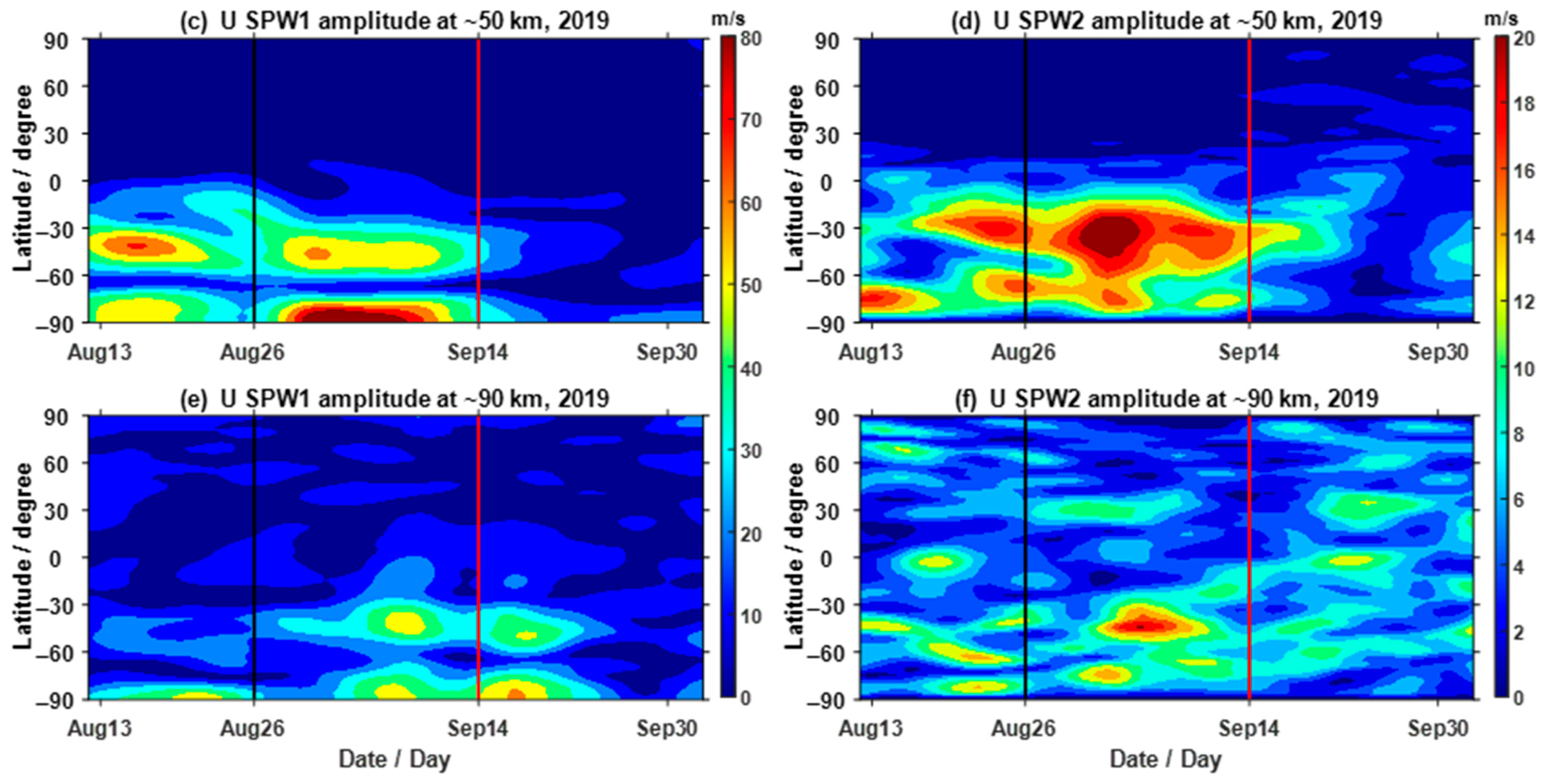
• This SSW was dominated by a strong SPW1 activity, and a weak increase in SPW2 also occurred during this SSW.
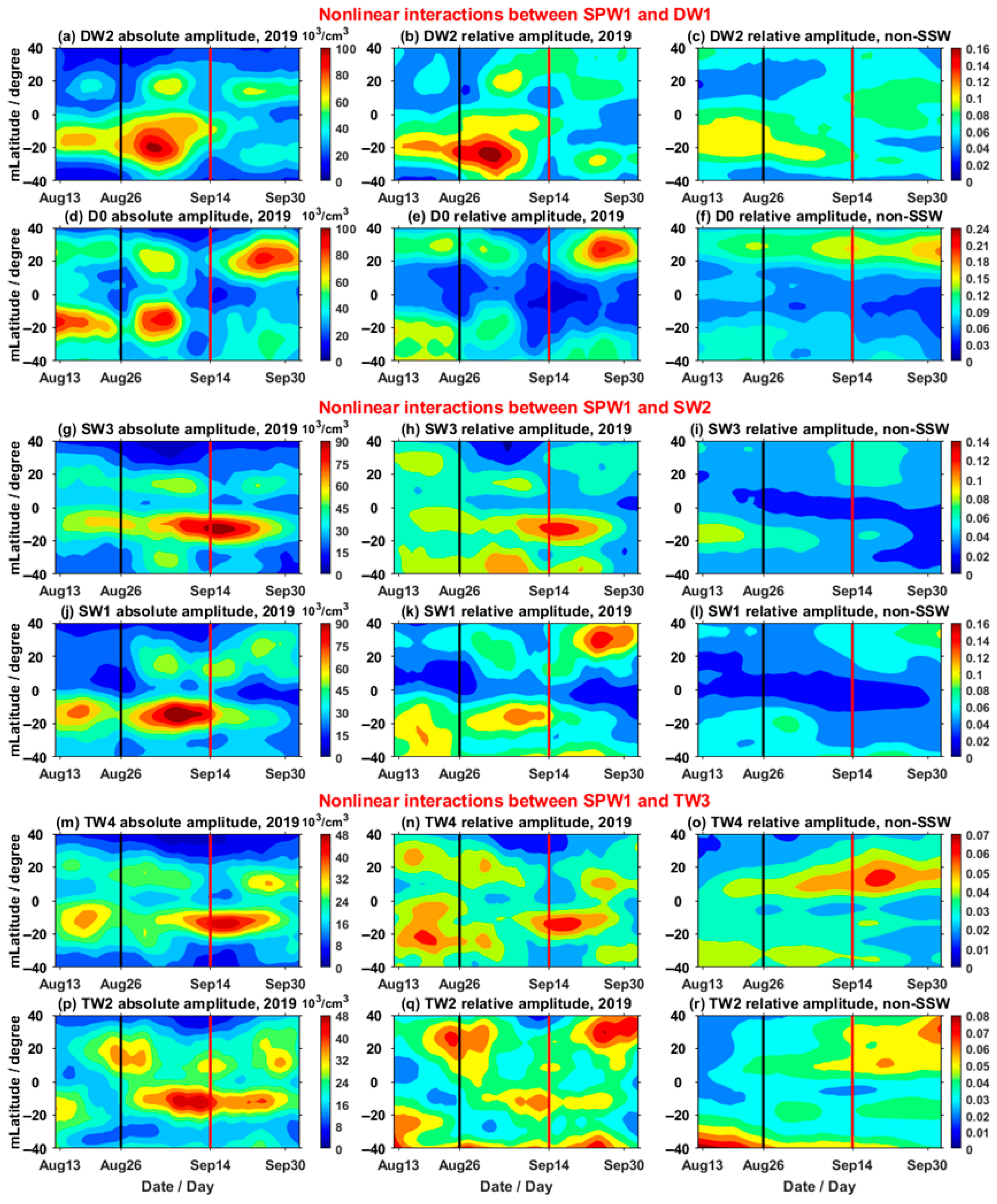
• Nonlinear interactions between SPW1 and migrating tides have also been triggered during this SSW event, which have significant influences on the corresponding nonmigrating tides. Also, these diurnal and semidiurnal nonmigrating tides, generated and influenced by the nonlinear interactions, show simultaneous enhancements in the neutral atmosphere and ionosphere.
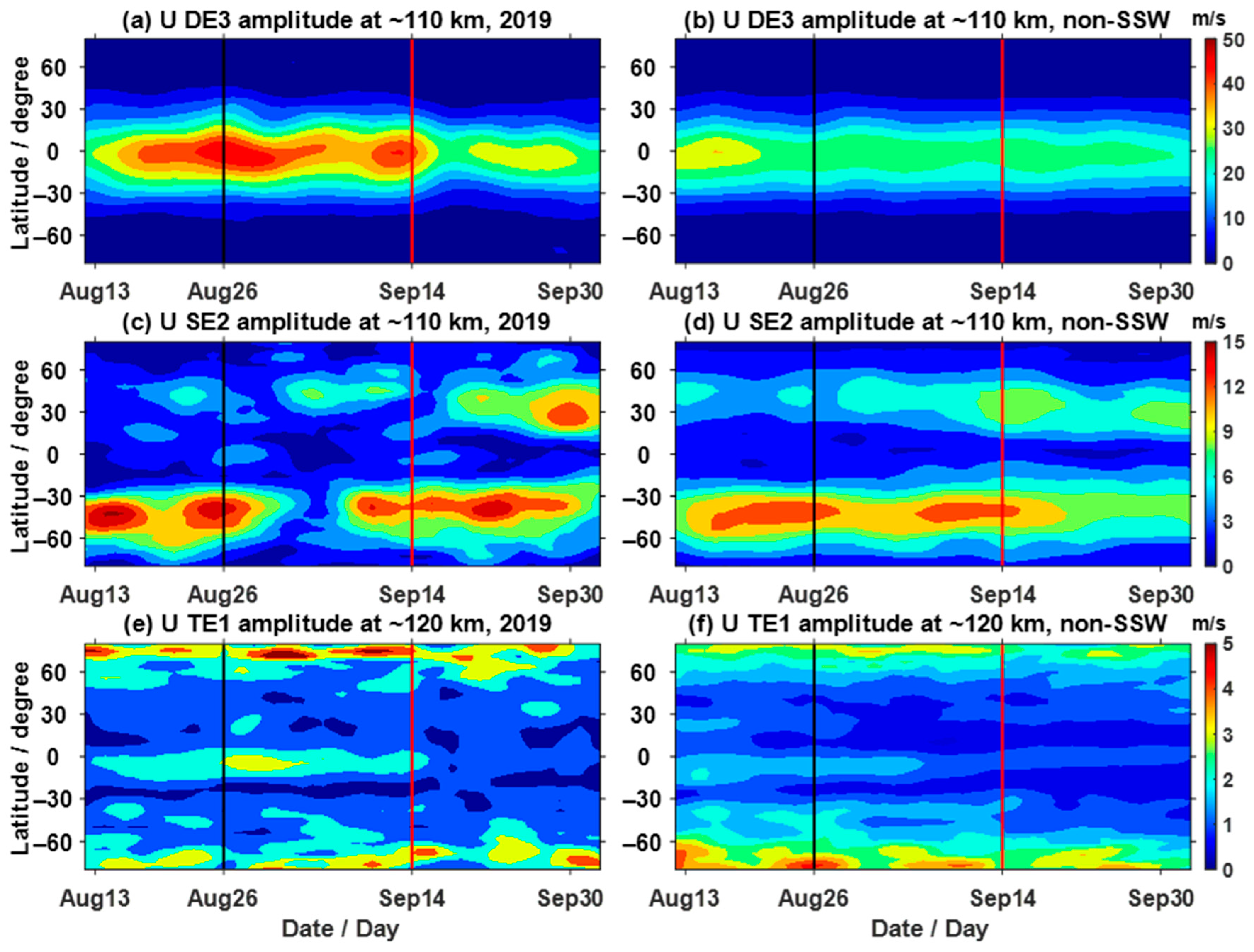
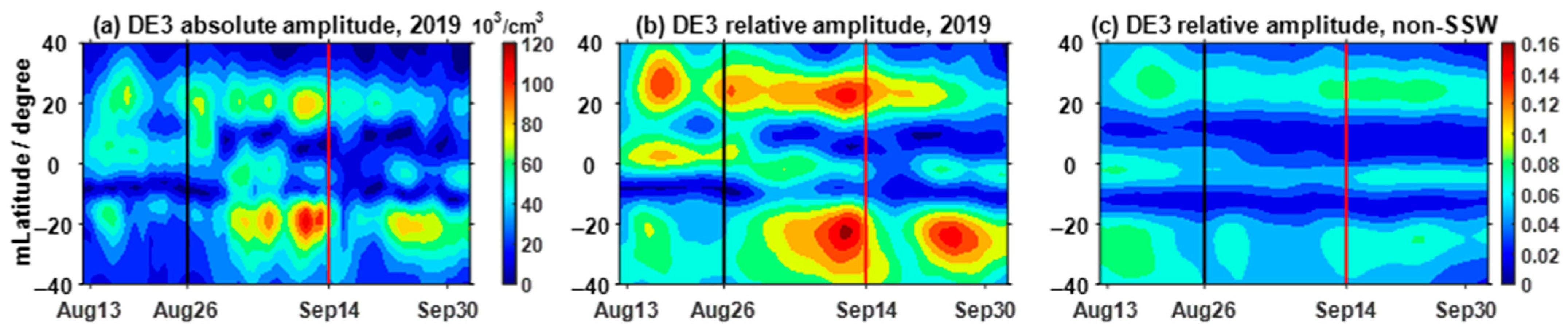
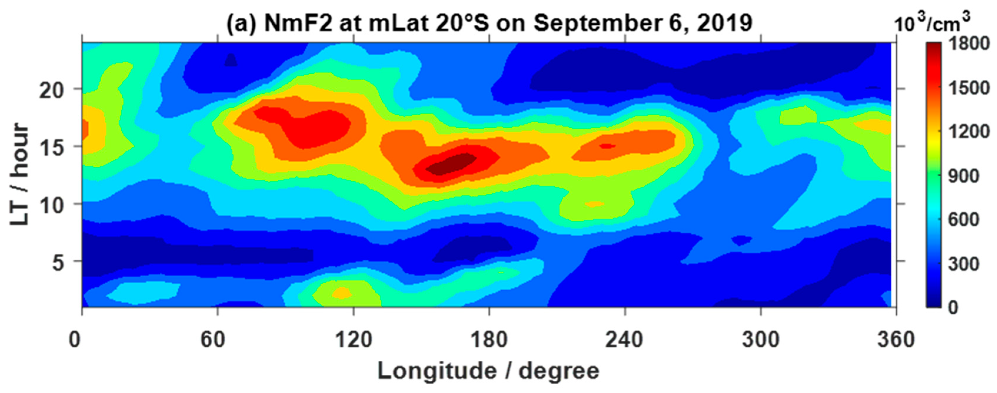
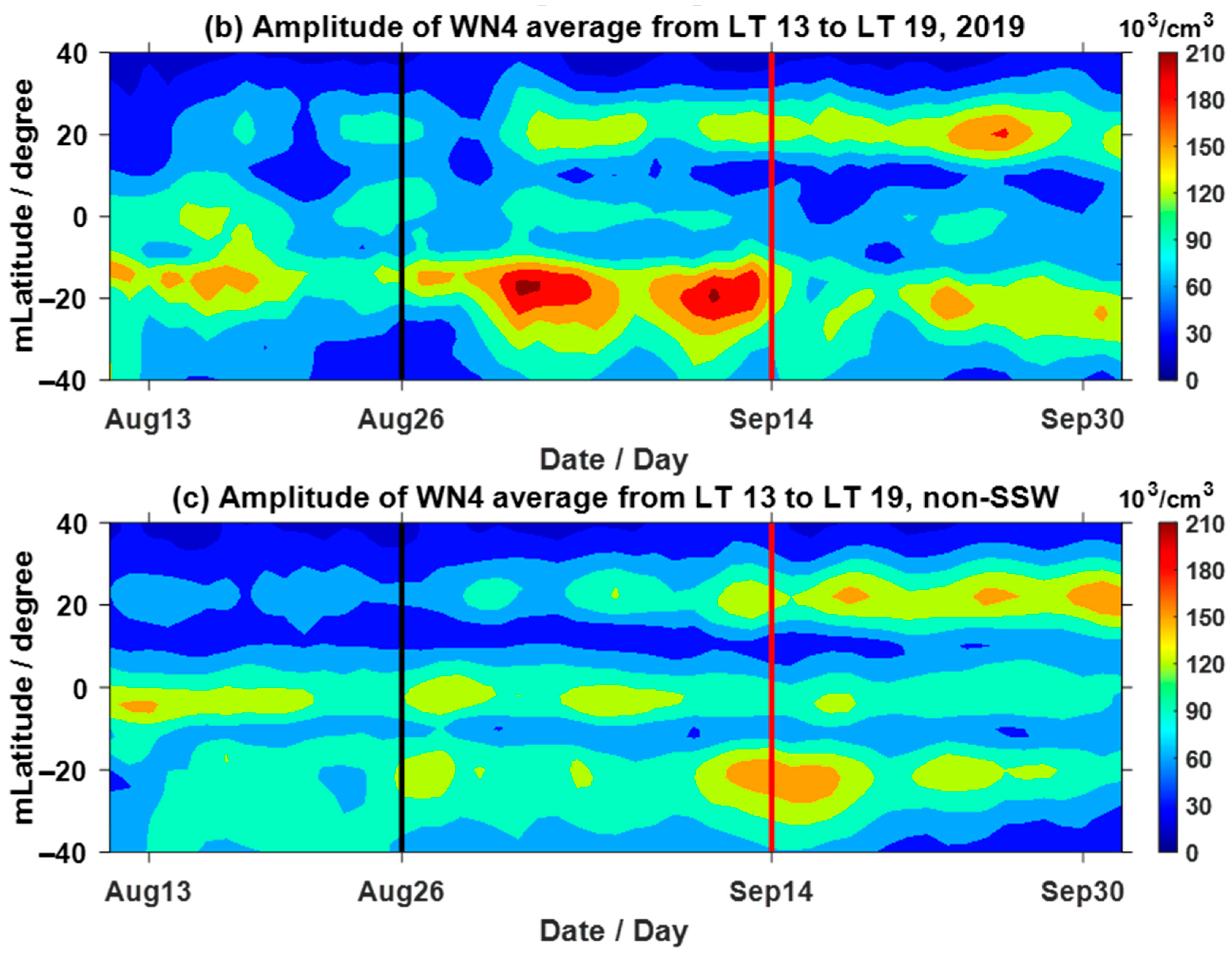
• The DE3, SE2 and TE1 have significant concurrent increases in the neutral atmosphere and ionosphere, and the amplitudes of the ionospheric longitudinal WN4 structure also show simultaneous increases. This indicates that the ionospheric longitudinal WN4 structure was influenced by these three nonmigrating tides during this SSW, and the influence of DE3 was the strongest.

Our analysis clearly demonstrates that the ionosphere can be influenced by the variations of nonmigrating tides, which results from nonlinear interactions, and that an SSW may serve as a great trigger for the short-term ionospheric variabilities.

References

1. Andrews, D.G.; Holton, J.R.; Leovy, C.B. Middle Atmosphere Dynamics; Academic Press: Orlando, FL, USA, 1987; pp. xi, 489. [Google Scholar]
2. Butler, A.H.; Seidel, D.J.; Hardiman, S.C.; Butchart, N.; Birner, T.; Match, A. Defining Sudden Stratospheric Warmings. Bull. Am. Meteorol. Soc. 2015, 96, 1913–1928. [Google Scholar] [CrossRef]
3. Butler, A.H.; Sjoberg, J.P.; Seidel, D.J.; Rosenlof, K.H. A sudden stratospheric warming compendium. Earth Syst. Sci. Data 2017, 9, 63–76. [Google Scholar] [CrossRef]
4. Matsuno, T. A Dynamical Model of the Stratospheric Sudden Warming. J. Atmos. Sci. 1971, 28, 1479–1494. [Google Scholar] [CrossRef]
5. van Loon, H.; Jenne, R.L.; Labitzke, K. Zonal harmonic standing waves. J. Geophys. Res. 1973, 78, 4463–4471. [Google Scholar] [CrossRef]
6. Yamazaki, Y.; Matthias, V.; Miyoshi, Y.; Stolle, C.; Siddiqui, T.; Kervalishvili, G.; Laštovička, J.; Kozubek, M.; Ward, W.; Themens, D.R.; et al. September 2019 Antarctic Sudden Stratospheric Warming: Quasi-6-Day Wave Burst and Ionospheric Effects. Geophys. Res. Lett. 2020, 47, e2019GL086577. [Google Scholar] [CrossRef]
7. Gu, S.Y.; Teng, C.K.M.; Li, N.; Jia, M.; Li, G.; Xie, H.; Ding, Z.; Dou, X. Multivariate Analysis on the Ionospheric Responses to Planetary Waves During the 2019 Antarctic SSW Event. J. Geophys. Res.-Space Phys. 2021, 126, e2020JA028588. [Google Scholar] [CrossRef]
8. Chandran, A.; Collins, R.L. Stratospheric sudden warming effects on winds and temperature in the middle atmosphere at middle and low latitudes: A study using WACCM. Ann. Geophys. 2014, 32, 859–874. [Google Scholar] [CrossRef]
9. Goncharenko, L.P.; Chau, J.L.; Liu, H.L.; Coster, A.J. Unexpected connections between the stratosphere and ionosphere. Geophys. Res. Lett. 2010, 37, L10101. [Google Scholar] [CrossRef]
10. Liu, H.X.; Miyoshi, Y.; Miyahara, S.; Jin, H.; Fujiwara, H.; Shinagawa, H. Thermal and dynamical changes of the zonal mean state of the thermosphere during the 2009 SSW: GAIA simulations. J. Geophys. Res. Space Phys. 2014, 119, 6784–6791. [Google Scholar] [CrossRef]
11. Fuller-Rowell, T.; Akmaev, R.; Wu, F.; Fedrizzi, M.; Viereck, R.A.; Wang, H.J. Did the January 2009 sudden stratospheric warming cool or warm the thermosphere? Geophys. Res. Lett. 2011, 38, L18104. [Google Scholar] [CrossRef]
12. Baldwin, M.P.; Ayarzaguena, B.; Birner, T.; Butchart, N.; Butler, A.H.; Charlton-Perez, A.J.; Domeisen, D.I.V.; Garfinkel, C.I.; Garny, H.; Gerber, E.P.; et al. Sudden Stratospheric Warmings. Rev. Geophys. 2021, 59, e2020RG000708. [Google Scholar] [CrossRef]
13. Forbes, J.M. Tidal and Planetary Waves. In The Upper Mesosphere and Lower Thermosphere: A Review of Experiment and Theory; Geophysical Monograph Series; American Geophysical Union: Washington, DC, USA, 1995; pp. 67–87. [Google Scholar]
14. Lindzen, R.S.; Chapman, S.J. Atmospheric tides. Space Sci. Rev. 1969, 10, 3–188. [Google Scholar]
15. Goncharenko, L.P.; Coster, A.J.; Chau, J.L.; Valladares, C.E. Impact of sudden stratospheric warmings on equatorial ionization anomaly. J. Geophys. Res. Space Phys. 2010, 115, A00g07. [Google Scholar] [CrossRef]
16. Pedatella, N.M.; Liu, H.L. The influence of atmospheric tide and planetary wave variability during sudden stratosphere warmings on the low latitude ionosphere. J. Geophys. Res. Space Phys. 2013, 118, 5333–5347. [Google Scholar] [CrossRef]
17. Yasyukevich, A.S. Variations in Ionospheric Peak Electron Density During Sudden Stratospheric Warmings in the Arctic Region. J. Geophys. Res. Space Phys. 2018, 123, 3027–3038. [Google Scholar] [CrossRef]
18. Liu, H.L.; Roble, R.G. A study of a self-generated stratospheric sudden warming and its mesospheric-lower thermospheric impacts using the coupled TIME-GCM/CCM3. J. Geophys. Res. Atmos. 2002, 107, 4695. [Google Scholar] [CrossRef]
19. Liu, H.L.; Wang, W.; Richmond, A.D.; Roble, R.G. Ionospheric variability due to planetary waves and tides for solar minimum conditions. J. Geophys. Res. Space Phys. 2010, 115, A00g01. [Google Scholar] [CrossRef]
20. Sridharan, S.; Sathishkumar, S.; Gurubaran, S. Variabilities of mesospheric tides and equatorial electrojet strength during major stratospheric warming events. Ann. Geophys. 2009, 27, 4125–4130. [Google Scholar] [CrossRef]
21. Pedatella, N.M.; Richmond, A.D.; Maute, A.; Liu, H.L. Impact of semidiurnal tidal variability during SSWs on the mean state of the ionosphere and thermosphere. J. Geophys. Res. Space Phys. 2016, 121, 8077–8088. [Google Scholar] [CrossRef]
22. Yue, X.A.; Schreiner, W.S.; Lei, J.H.; Rocken, C.; Hunt, D.C.; Kuo, Y.H.; Wan, W.X. Global ionospheric response observed by COSMIC satellites during the January 2009 stratospheric sudden warming event. J. Geophys. Res. Space Phys. 2010, 115, A00g09. [Google Scholar] [CrossRef]
23. Pedatella, N.M.; Forbes, J.M. Evidence for stratosphere sudden warming-ionosphere coupling due to vertically propagating tides. Geophys. Res. Lett. 2010, 37, L11104. [Google Scholar] [CrossRef]
24. Fuller-Rowell, T.; Wu, F.; Akmaev, R.; Fang, T.W.; Araujo-Pradere, E. A whole atmosphere model simulation of the impact of a sudden stratospheric warming on thermosphere dynamics and electrodynamics. J. Geophys. Res. Space Phys. 2010, 115, A00g08. [Google Scholar] [CrossRef]
25. Jin, H.; Miyoshi, Y.; Pancheva, D.; Mukhtarov, P.; Fujiwara, H.; Shinagawa, H. Response of migrating tides to the stratospheric sudden warming in 2009 and their effects on the ionosphere studied by a whole atmosphere-ionosphere model GAIA with COSMIC and TIMED/SABER observations. J. Geophys. Res. Space Phys. 2012, 117, A10323. [Google Scholar] [CrossRef]
26. Eswaraiah, S.; Kim, Y.H.; Lee, J.; Ratnam, M.V.; Rao, S.V.B. Effect of Southern Hemisphere Sudden Stratospheric Warmings on Antarctica Mesospheric Tides: First Observational Study. J. Geophys. Res. Space Phys. 2018, 123, 2127–2140. [Google Scholar] [CrossRef]
27. Guharay, A.; Batista, P.P. On the variability of tides during a major stratospheric sudden warming in September 2002 at Southern hemispheric extra-tropical latitude. Adv. Space Res. 2019, 63, 2337–2344. [Google Scholar] [CrossRef]
28. Teng, C.K.M.; Gu, S.Y.; Qin, Y.; Dou, X.; Li, N.; Tang, L. Unexpected Decrease in TW3 Amplitude During Antarctic Sudden Stratospheric Warming Events as Revealed by SD-WACCM-X. J. Geophys. Res. Space Phys. 2021, 126, e2020JA029050. [Google Scholar] [CrossRef]
29. Eswaraiah, S.; Kim, J.H.; Lee, W.; Hwang, J.; Kumar, K.N.; Kim, Y.H. Unusual Changes in the Antarctic Middle Atmosphere During the 2019 Warming in the Southern Hemisphere. Geophys. Res. Lett. 2020, 47, e2020GL089199. [Google Scholar] [CrossRef]
30. Liu, H.L.; Roble, R.G. Dynamical coupling of the stratosphere and mesosphere in the 2002 Southern Hemisphere major stratospheric sudden warming. Geophys. Res. Lett. 2005, 32, L13804. [Google Scholar] [CrossRef]
31. Goncharenko, L.P.; Harvey, V.L.; Greer, K.R.; Zhang, S.R.; Coster, A.J. Longitudinally Dependent Low-Latitude Ionospheric Disturbances Linked to the Antarctic Sudden Stratospheric Warming of September 2019. J. Geophys. Res.-Space Phys. 2020, 125, e2020JA028199. [Google Scholar] [CrossRef]
32. Liu, G.; Janches, D.; Ma, J.; Lieberman, R.S.; Stober, G.; Moffat-Griffin, T.; Mitchell, N.J.; Kim, J.H.; Lee, C.; Murphy, D.J. Mesosphere and Lower Thermosphere Winds and Tidal Variations During the 2019 Antarctic Sudden Stratospheric Warming. J. Geophys. Res. Space Phys. 2022, 127, e2021JA030177. [Google Scholar] [CrossRef]
33. He, M.; Chau, J.L.; Forbes, J.M.; Thorsen, D.; Li, G.; Siddiqui, T.A.; Yamazaki, Y.; Hocking, W.K. Quasi-10-Day Wave and Semidiurnal Tide Nonlinear Interactions During the Southern Hemispheric SSW 2019 Observed in the Northern Hemispheric Mesosphere. Geophys. Res. Lett. 2020, 47, e2020GL091453. [Google Scholar] [CrossRef]
34. Yamazaki, Y.; Miyoshi, Y. Ionospheric Signatures of Secondary Waves from Quasi-6-Day Wave and Tide Interactions. J. Geophys. Res. Space Phys. 2021, 126, e2020JA028360. [Google Scholar] [CrossRef]
35. Li, N.; Lei, J.; Huang, F.; Yi, W.; Chen, J.; Xue, X.; Gu, S.; Luan, X.; Zhong, J.; Liu, F.; et al. Responses of the Ionosphere and Neutral Winds in the Mesosphere and Lower Thermosphere in the Asian-Australian Sector to the 2019 Southern Hemisphere Sudden Stratospheric Warming. J. Geophys. Res. Space Phys. 2021, 126, e2020JA028653. [Google Scholar] [CrossRef]
36. Limpasuvan, V.; Richter, J.H.; Orsolini, Y.J.; Stordal, F.; Kvissel, O.K. The roles of planetary and gravity waves during a major stratospheric sudden warming as characterized in WACCM. J. Atmos. Sol. Terr. Phys. 2012, 78–79, 84–98. [Google Scholar] [CrossRef]
37. Qin, Y.; Gu, S.Y.; Teng, C.K.M.; Dou, X.K.; Yu, Y.; Li, N. Comprehensive Study of the Climatology of the Quasi-6-Day Wave in the MLT Region Based on Aura/MLS Observations and SD-WACCM-X Simulations. J. Geophys. Res.-Space Phys. 2020, 126, e2020JA028454. [Google Scholar] [CrossRef]
38. Sassi, F.; Liu, H.L.; Ma, J.; Garcia, R.R. The lower thermosphere during the northern hemisphere winter of 2009: A modeling study using high-altitude data assimilation products in WACCM-X. J. Geophys. Res.Atmos. 2013, 118, 8954–8968. [Google Scholar] [CrossRef]
39. McDonald, S.E.; Sassi, F.; Mannucci, A.J. SAMI3/SD-WACCM-X simulations of ionospheric variability during northern winter 2009. Space Weather. Int. J. Res. Appl. 2015, 13, 568–584. [Google Scholar] [CrossRef]
40. Sassi, F.; Siskind, D.E.; Tate, J.L.; Liu, H.L.; Randall, C.E. Simulations of the Boreal Winter Upper Mesosphere and Lower Thermosphere with Meteorological Specifications in SD-WACCM-X. J. Geophys. Res. Atmos. 2018, 123, 3791–3811. [Google Scholar] [CrossRef]
41. Liu, H.L.; Foster, B.T.; Hagan, M.E.; McInerney, J.M.; Maute, A.; Qian, L.; Richmond, A.D.; Roble, R.G.; Solomon, S.C.; Garcia, R.R.; et al. Thermosphere extension of the Whole Atmosphere Community Climate Model. J. Geophys. Res. Space 2010, 115, A12302. [Google Scholar] [CrossRef]
42. Liu, H.L.; Bardeen, C.G.; Foster, B.T.; Lauritzen, P.H.; Liu, J.; Lu, G.; Marsh, D.R.; Maute, A.; McInerney, J.M.; Pedatella, N.M.; et al. Development and Validation of the Whole Atmosphere Community Climate Model with Thermosphere and Ionosphere Extension (WACCM-X 2.0). J. Adv. Model. Earth Syst. 2018, 10, 381–402. [Google Scholar] [CrossRef]
43. Marsh, D.R. Chemical–Dynamical Coupling in the Mesosphere and Lower Thermosphere. In Aeronomy of the Earth's Atmosphere and Ionosphere; Abdu, M.A., Pancheva, D., Eds.; Springer: Dordrecht, The Netherlands, 2011; pp. 3–17. [Google Scholar]
44. Pancheva, D.; Mukhtarov, P.; Hall, C.; Meek, C.; Tsutsumi, M.; Pedatella, N.; Nozawa, S. Climatology of the main (24-h and 12-h) tides observed by meteor radars at Svalbard and Tromsø: Comparison with the models CMAM-DAS and WACCM-X. J. Atmos. Sol.-Terr. Phys. 2020, 207, 105339. [Google Scholar] [CrossRef]
45. Zhang, J.; Limpasuvan, V.; Orsolini, Y.J.; Espy, P.J.; Hibbins, R.E. Climatological Westward-Propagating Semidiurnal Tides and Their Composite Response to Sudden Stratospheric Warmings in SuperDARN and SD-WACCM-X. J. Geophys. Res. Atmos. 2021, 126, e2020JD032895. [Google Scholar] [CrossRef]
46. Wu, D.L.; Hays, P.B.; Skinner, W.R. A Least-Squares Method for Spectral-Analysis of Space-Time Series. J. Atmos. Sci. 1995, 52, 3501–3511. [Google Scholar] [CrossRef]
47. Pancheva, D.; Mukhtarov, P.; Andonov, B.; Mitchell, N.J.; Forbes, J.M. Planetary waves observed by TIMED/SABER in coupling the stratosphere–mesosphere–lower thermosphere during the winter of 2003/2004: Part 1—Comparison with the UKMO temperature results. J. Atmos. Sol.-Terr. Phys. 2009, 71, 61–74. [Google Scholar] [CrossRef]
48. Teitelbaum, H.; Vial, F. On Tidal Variability Induced by Nonlinear-Interaction with Planetary-Waves. J. Geophys. Res. Space 1991, 96, 14169–14178. [Google Scholar] [CrossRef]
49. Smith, A.K. Observation of Wave-Wave Interactions in the Stratosphere. J. Atmos. Sci. 1983, 40, 2484–2496. [Google Scholar] [CrossRef]
50. Miyoshi, Y.; Yamazaki, Y. Excitation Mechanism of Ionospheric 6-Day Oscillation During the 2019 September Sudden Stratospheric Warming Event. J. Geophys. Res. Space Phys. 2020, 125, e2020JA028283. [Google Scholar] [CrossRef]
51. Sridharan, S. Variabilities of Low-Latitude Migrating and Nonmigrating Tides in GPS-TEC and TIMED-SABER Temperature During the Sudden Stratospheric Warming Event of 2013. J. Geophys. Res. Space 2017, 122, 10748–10761. [Google Scholar] [CrossRef]
52. Pancheva, D.; Mukhtarov, P.; Andonov, B. Nonmigrating tidal activity related to the sudden stratospheric warming in the Arctic winter of 2003/2004. Ann. Geophys. 2009, 27, 975–987. [Google Scholar] [CrossRef]
53. Maute, A.; Hagan, M.E.; Richmond, A.D.; Roble, R.G. TIME-GCM study of the ionospheric equatorial vertical drift changes during the 2006 stratospheric sudden warming. J. Geophys. Res. Space 2014, 119, 1287–1305. [Google Scholar] [CrossRef]
54. Forbes, J.M.; Russell, J.; Miyahara, S.; Zhang, X.; Palo, S.; Mlynczak, M.; Mertens, C.J.; Hagan, M.E. Troposphere-thermosphere tidal coupling as measured by the SABER instrument on TIMED during July-September 2002. J. Geophys. Res. Space 2006, 111, A10s06. [Google Scholar] [CrossRef]
55. Liu, G.; Lieberman, R.S.; Harvey, V.L.; Pedatella, N.M.; Oberheide, J.; Hibbins, R.E.; Espy, P.J.; Janches, D. Tidal Variations in the Mesosphere and Lower Thermosphere Before, During, and After the 2009 Sudden Stratospheric Warming. J. Geophys. Res. Space Phys. 2021, 126, e2020JA028827. [Google Scholar] [CrossRef]
56. Xu, J.Y.; Smith, A.K.; Liu, M.H.; Liu, X.; Gao, H.; Jiang, G.Y.; Yuan, W. Evidence for nonmigrating tides produced by the interaction between tides and stationary planetary waves in the stratosphere and lower mesosphere. J. Geophys. Res. Atmos. 2014, 119, 471–489. [Google Scholar] [CrossRef]
57. Lieberman, R.S.; Riggin, D.M.; Ortland, D.A.; Oberheide, J.; Siskind, D.E. Global observations and modeling of nonmigrating diurnal tides generated by tide-planetary wave interactions. J. Geophys. Res. Atmos. 2015, 120, 11419–11437. [Google Scholar] [CrossRef]
58. Niu, X.J.; Du, J.; Zhu, X.W. Statistics on Nonmigrating Diurnal Tides Generated by Tide-Planetary Wave Interaction and Their Relationship to Sudden Stratospheric Warming. Atmosphere 2018, 9, 416. [Google Scholar] [CrossRef]
59. Chang, L.C.; Palo, S.E.; Liu, H.L. Short-term variation of the s1 nonmigrating semidiurnal tide during the 2002 stratospheric sudden warming. J. Geophys. Res. Atmos. 2009, 114, D03109. [Google Scholar] [CrossRef]
60. Wan, W.; Ren, Z.; Ding, F.; Xiong, J.; Liu, L.; Ning, B.; Zhao, B.; Li, G.; Zhang, M.L. A simulation study for the couplings between DE3 tide and longitudinal WN4 structure in the thermosphere and ionosphere. J. Atmos. Sol.-Terr. Phys. 2012, 90–91, 52–60. [Google Scholar] [CrossRef]
61. Pedatella, N.M.; Hagan, M.E.; Maute, A. The comparative importance of DE3, SE2, and SPW4 on the generation of wave-number-4 longitude structures in the low-latitude ionosphere during September equinox. Geophys. Res. Lett. 2012, 39, L19108. [Google Scholar] [CrossRef]
62. Onohara, A.N.; Batista, I.S.; Batista, P.P. Wavenumber-4 structures observed in the low-latitude ionosphere during low and high solar activity periods using FORMOSAT/COSMIC observations. Ann. Geophys. 2018, 36, 459–471. [Google Scholar] [CrossRef]
63. Li, X.; Wan, W.X.; Cao, J.B.; Ren, Z.P. Wavenumber-4 spectral component extracted from TIMED/SABER observations. Earth Planet. Phys. 2020, 4, 436–448. [Google Scholar] [CrossRef]
64. Miyoshi, Y.; Jin, H.; Fujiwara, H.; Shinagawa, H.; Liu, H.X. Wave-4 structure of the neutral density in the thermosphere and its relation to atmospheric tides. J. Atmos. Sol. Terr. Phys. 2012, 90–91, 45–51. [Google Scholar] [CrossRef]
Figure 1. Average spatial structures of the (a) SPW1 and (b) SPW2 in zonal wind from 26 August to 14 September 2019. Temporal and latitudinal variations of the (c,e) SPW1 and (d,f) SPW2 amplitude in zonal wind at (c,d) ~50 km and (e,f) ~90 km. The black and red vertical solid lines in (cf) indicate the onset day of the SSW and the day on which the temperature reached its maximum during the 2019 Antarctic SSW, respectively.
Atmosphere 16 00848 g001aAtmosphere 16 00848 g001b
Figure 2. Wavenumber and latitudinal variations of (a,b) diurnal, (c,d) semidiurnal and (e,f) terdiurnal tidal amplitudes in (a,c,e) SD-WACCM-X and (b,d,f) SABER temperature at ~109 km averaged from 26 August to 14 September 2019.
Atmosphere 16 00848 g002aAtmosphere 16 00848 g002b
Figure 3. (a) Temporal and latitudinal variations of the SPW1 amplitude in zonal wind at ~90 km. Temporal and latitudinal variations of nonmigrating tides, which can be generated and influenced by nonlinear interactions between SPW1 and migrating tides, are exhibited, including (b,c) DW2 amplitude at ~100 km, (d,e) D0 amplitude at ~100 km, (f,g) SW3 amplitude at ~110 km, (h,i) SW1 amplitude at ~110 km, (j,k) TW4 amplitude at ~120 km and (l,m) TW2 amplitude at ~100 km in zonal wind during the (b,d,f,h,j,l) 2019 Antarctic SSW and (c,e,g,i,k,m) non-SSW period (average from 2014 to 2018). The black and red vertical solid lines indicate the onset day of the SSW and the day on which the temperature reached its maximum during the 2019 Antarctic SSW, respectively.
Atmosphere 16 00848 g003aAtmosphere 16 00848 g003b
Figure 4. Temporal and latitudinal variations of the (a,b) DE3 amplitude at ~110 km, (c,d) SE2 amplitude at ~110 km and (e,f) TE1 amplitude at ~120 km in zonal wind during the (a,c,e) 2019 Antarctic SSW and (b,d,f) non-SSW period (average from 2014 to 2018). The black and red vertical solid lines indicate the onset day of the SSW and the day on which the temperature reaches its maximum during the 2019 Antarctic SSW, respectively.
Atmosphere 16 00848 g004
Figure 5. Temporal and latitudinal variations of nonmigrating tidal absolute and relative amplitudes, which can be generated and influenced by nonlinear interactions between SPW1 and migrating tides, are exhibited, including (ac) DW2, (df) D0, (gi) SW3, (jl) SW1, (mo) TW4 and (pr) TW2 in NmF2 during the 2019 Antarctic SSW and non-SSW period (average from 2014 to 2018). The black and red vertical solid lines indicate the onset day of the SSW and the day on which the temperature reaches its maximum during the 2019 Antarctic SSW, respectively.
Atmosphere 16 00848 g005
Figure 6. Same as Figure 5, but for DE3, SE2 and TE1.
Atmosphere 16 00848 g006aAtmosphere 16 00848 g006b
Figure 7. (a) Longitude–local time distribution of NmF2 at magnetic latitude 20° S on 6 September 2019. Temporal variations of ionospheric longitudinal wavenumber 4 component amplitudes extracted from NmF2 average from LT 13 to LT 19 during the (b) 2019 Antarctic SSW and (c) non-SSW period (average from 2014 to 2018). The black and red vertical solid lines indicate the onset day of the SSW and the day on which the temperature reaches its maximum during the 2019 Antarctic SSW, respectively.
Atmosphere 16 00848 g007aAtmosphere 16 00848 g007b
Disclaimer/Publisher’s Note: The statements, opinions and data contained in all publications are solely those of the individual author(s) and contributor(s) and not of MDPI and/or the editor(s). MDPI and/or the editor(s) disclaim responsibility for any injury to people or property resulting from any ideas, methods, instructions or products referred to in the content.