Article

Ionospheric Response to the Extreme Geomagnetic Storm of 10–11 May 2024 Based on Total Electron Content Observations in the Central Asian and East Asian Regions

1
Institute of the Ionosphere, Almaty 050020, Kazakhstan
2
Department of Electrical and Electronics Engineering, Hacettepe University, Beytepe, Ankara 06230, Türkiye
*
Author to whom correspondence should be addressed.
Atmosphere 2025, 16(7), 854; https://doi.org/10.3390/atmos16070854 (registering DOI)
Submission received: 20 April 2025 / Revised: 1 July 2025 / Accepted: 7 July 2025 / Published: 14 July 2025
(This article belongs to the Special Issue Ionospheric Disturbances and Space Weather)

Abstract

The ionospheric response to the major geomagnetic storm (SYM-H = −518 nT) of 10–11 May 2024 was investigated using total electron content (TEC) observations from the Central Asian (CAR) and East Asian (EAR) regions. In the CAR region, shortly after the storm sudden commencement (SC) (17:05 UT on 10 May), during a rapid decrease in SYM-H, a significant TEC decrease (~70%) and a subsequent formation of a prolonged TEC depletion phase on 11 May were observed. The duration of the phase’s maximum intensity seemed to agree with the duration of southward interplanetary magnetic field (IMF) Bz activity. The total duration of the negative phase exceeded 3 days and correlated with the duration of the Auroral Electrojet (AE) index activity. The ionospheric response in the EAR region differed significantly, exhibiting a secondary, deeper TEC decrease (termed “phase 2”) on 12 May, which occurred during a period of reduced AE and IMF Bz activity. The analysis of latitudinal TEC variations in the EAR region revealed that “phase 2” occurred across a geographic latitude range of 31.4° N to 43.9° N (approximately 21° N to 34° N dipole latitude). These results are discussed in the context of potential longitudinal variations in thermospheric composition and meridional circulation during the geomagnetic storm.

1. Introduction

The influence of solar eruptive and radiative processes on the near-Earth space environment has been investigated for decades to understand the mechanisms through which solar activity affects processes within the Earth’s atmosphere, thermosphere, and ionosphere [1,2]. Due to the increasing demand for near-Earth operations with low Earth orbit and middle Earth orbit satellites for monitoring, positioning, and navigation, the geomagnetic variability of the ionosphere and plasmasphere is the subject of utmost academic attention. Studies focusing on extreme solar events, such as flares and coronal mass ejections (CMEs), are particularly important. These events often lead to extended periods of heightened geomagnetic activity and energetic particle precipitation, causing significant changes in the thermosphere/ionosphere and impacting technologically advanced ground-based and space-borne systems [3,4]. Examples illustrate the potential severity: a powerful Earth-directed solar event can significantly disrupt terrestrial systems. Notable instances include the degradation of Global Positioning System (GPS) navigation performance during geomagnetically disturbed conditions [5,6]; the electric power blackout in Quebec, Canada, during the 13–15 March 1989 storm [7]; the electric power blackout in southern Sweden on 30 October 2003 [8]; and the loss of thirty-eight Starlink satellites due to a geomagnetic storm on 4 February 2022, resulting in significant financial and aerospace consequences [9]. These incidents underscore the need for continued study to better understand the characteristics and evolution of extreme space weather events.
The geomagnetic storm of 10–11 May 2024 has recently received considerable attention [10,11,12,13,14,15,16,17,18,19]. The storm impacted power grids, disrupted precision navigation systems, and generated widespread auroral displays. It significantly affected the composition, temperature, and dynamics of the Earth’s thermosphere, as observed by the Global-Scale Observations of the Limb and Disk (GOLD) instrument [11]. The GOLD revealed significant thermospheric heating, a decrease in the column-integrated O/N2 ratio (ΣO/N2) at high latitudes, and a complex morphology in temperature and ΣO/N2 at mid- and equatorial latitudes. The authors of [11] attributed the latter to potential longitudinal variations in meridional winds; however, a lack of direct wind measurements precluded confirmation of this hypothesis.
Several studies have examined the ionospheric response to the 10–11 May 2024 geomagnetic storm in various geographical regions [9,10,11,12,13,14,15,16,17]. For instance, analyzing global ionospheric total electron content (TEC) maps, Ram et al. [12] reported a substantial ionospheric disturbance, including a TEC increase exceeding 100% during the daytime on 10 May in the American longitudinal sector (75° W). They showed that this TEC enhancement occurred from low to mid-latitudes (±45°) in both hemispheres, resulting from the intensification and poleward expansion of the Equatorial Ionization Anomaly (EIA) crests. Similarly, Singh et al. [13], analyzing GPS TEC data over the American sector and incoherent scatter radar data from Jicamarca, Peru, observed an anomalous enhancement and expansion of the EIA to mid-latitudes (up to 38° N and 50° S). They reported large TEC increases during the afternoon and nighttime of 10 May at low and mid-latitudes (up to 1325% in the Southern Hemisphere and 380% in the Northern Hemisphere), persisting for approximately 8 h until 23:00 LT over the Americas.
In contrast, Kwak et al. [15] investigated the ionospheric response using ionosonde (foF2) and GNSS TEC data from stations in the East Asian region (Korea, Japan; 127.1° E–141.8° E, ~22.5° N–37.4° N dipole latitude). Their observations indicated a strong negative ionospheric storm effect, characterized by significant decreases and intense fluctuations in foF2 and TEC on 11 May. Jain et al. [16] also reported a dominant negative phase on 11 May using GPS TEC data from the Indian region (Bhopal, 14.2° N GMLAT), with a maximum deviation of approximately −68.5% around 20:45 UT. However, they also observed positive effects, including a +61% deviation around 05:00 UT on 12 May, TEC enhancements (24% to 50%) during the main phase, and quasi-periodic structures on 12 May, interpreted as signatures of prompt penetration electric fields and storm-induced traveling ionospheric disturbances (TIDs). Pierrard et al. [17], using GPS TEC data over Europe, observed an initial brief ionization increase followed by a rapid and prolonged TEC decrease from 10 to 12 May across northern (61° N), middle (50.5° N), and lower European latitudes (36° N).
These studies indicate that the 10–11 May 2024 extreme geomagnetic storm caused significant spatiotemporal ionospheric variations, exhibiting complex morphology dependent on geographic location. A comprehensive understanding of the global ionospheric disturbance necessitates analyzing data from diverse regions. This study aims to investigate the ionospheric response to this major geomagnetic storm (SYM-H minimum = −518 nT) using TEC data from the Central Asian (Chumish station) and East Asian (Sheshan, Fangshan, Chungchan, and Daejeon stations) regions.
Section 2 describes the data and methods. Section 3 presents the results and discussion. Section 4 provides the conclusions.

2. Materials and Methods

The ionospheric response to the 10–11 May 2024 geomagnetic storm was investigated using total electron content (TEC) data derived from Global Positioning System (GPS) receivers located at stations in the Central Asian (CAR) and East Asian (EAR) regions (Table 1). The geographic coordinates of the stations were obtained via the Nevada Geodetic Laboratory service (https://geodesy.unr.edu/NGLStationPages/GlobalStationList, accessed on 7 July 2025). The geomagnetic latitudes were calculated according to the geographic coordinates of the stations using the IRI-Plas model via the IONOLAB service (Department of Electrical and Electronics Engineering, Hacettepe University, Ankara, Türkiye; http://www.ionolab.org).
TEC is defined as the line integral of electron density along the path between the satellite and the receiver. It corresponds to the total number of electrons in a column of 1 m2 cross-section. The unit of TEC is TECu, and 1 TECu = 1016 el/m2. TEC has been widely recognized as a reliable indicator of ionospheric variability, and the cost-effective estimation of TEC using GPS data has been used in ionospheric studies since 1998.
The TEC values in this study were estimated using IONOLAB-TEC software (v1-41), which is available both online at www.ionolab.org and is also in an executable file form that can be downloaded to local computers. The online version requires only the date and the GPS receiver station name that can be chosen from the pop-up map. It automatically downloads the necessary RINEX, IONEX, and Ephemeris files, and the estimated TEC can be viewed and compared with the TEC estimates of IGS Ionospheric Analysis Centers. The manual for operating the executable file is provided along with a detailed description. If desired, the Slant TEC values can also be viewed in an executable file form on the user’s computer. The executable file also works automatically on the user’s computer, requiring only the date and file depository address. All other necessary files were downloaded in a user-friendly manner. The output files were written into user-defined directories. In this manner, the IONOLAB-TEC used in this study was generated by entering the station names and dates on the website or in the user-defined directories on their computer. The main algorithm of IONOLAB-TEC is the scientifically reproducible Reg-Est algorithm, as discussed in detail in [20]. If the user wants to write the code by themselves, then all of the equations are provided in the open literature. The Reg-Est is a robust method developed for estimating vertical total electron content (VTEC) from GPS measurements at a high temporal resolution of 30 s. Its function involves combining slant TEC data, derived from either pseudo-range or the less noisy phase-corrected measurements, gathered from all GPS satellites visible above a 10° horizon limit at a specific receiver location over a desired period [21]. The algorithm operates by minimizing a cost function through a least-squares approach; this function incorporates a high-pass penalty filter, enabling the accurate representation of sharp, sudden temporal variations in the ionosphere. Furthermore, Reg-Est can utilize optional weighting functions to mitigate multipath effects, particularly from low-elevation satellites, and appropriately handle differential code biases [22]. The algorithm uses IONOLAB-BIAS for receiver differential code bias estimation [23]. IONOLAB-TEC provides robust, high-resolution TEC values that capture important temporal features across diverse geomagnetic conditions and various geographic locations. Essentially, IONOLAB-TEC offers the detailed computational technique necessary for deriving high-fidelity TEC values from raw GPS data, likely serving as the foundation for services that provide accurate TEC products, such as those potentially offered by IONOLAB-TEC online to all researchers at www.ionolab.org, either as a downloadable executable file or online through a user-friendly interface [24]. The data used in this study were obtained via the IONOLAB service (Department of Electrical and Electronics Engineering, Hacettepe University, Ankara, Türkiye; http://www.ionolab.org), with a temporal resolution of 2.5 min. IONOLAB-TEC has been used in various studies, and it is one of the most cited contributions to this area. The ability of IONOLAB-TEC to estimate single station TEC with significant accuracy, reliability, and robustness has made it one of the most important software programs used in a wide variety of applications, including but not limited to modeling, mapping, and tomography [22,23,24].
The analysis period spanned 10–14 May 2024, with 9 May 2024 selected as a geomagnetically quiet reference day (Ap = 5, Kp = 1.3). Solar wind parameters and interplanetary magnetic field (IMF) data were used to characterize the drivers of the storm. Specifically, data on the total IMF strength (Bt), the north–south IMF component (IMF-Bz), solar wind speed (Vsw), and solar wind dynamic pressure (Pdyn) were obtained from the NASA/GSFC OMNIWeb database (https://omniweb.gsfc.nasa.gov/form/omni_min.html, accessed on 7 July 22025). Geomagnetic conditions were assessed using the planetary Ap and Kp indices, the Auroral Electrojet (AE) index, and the symmetric horizontal component (SYM-H) index, also sourced from the OMNIWeb database. The general space weather context for May 2024 was obtained from NOAA/SWPC weekly reports (ftp://ftp.ngdc.noaa.gov/STP/swpc_products/weekly_reports/, accessed on 7 July 2025) and SpaceWeather.com (http://spaceweather.com). In the next section, we provide detailed results and discussion.

3. Results and Discussion

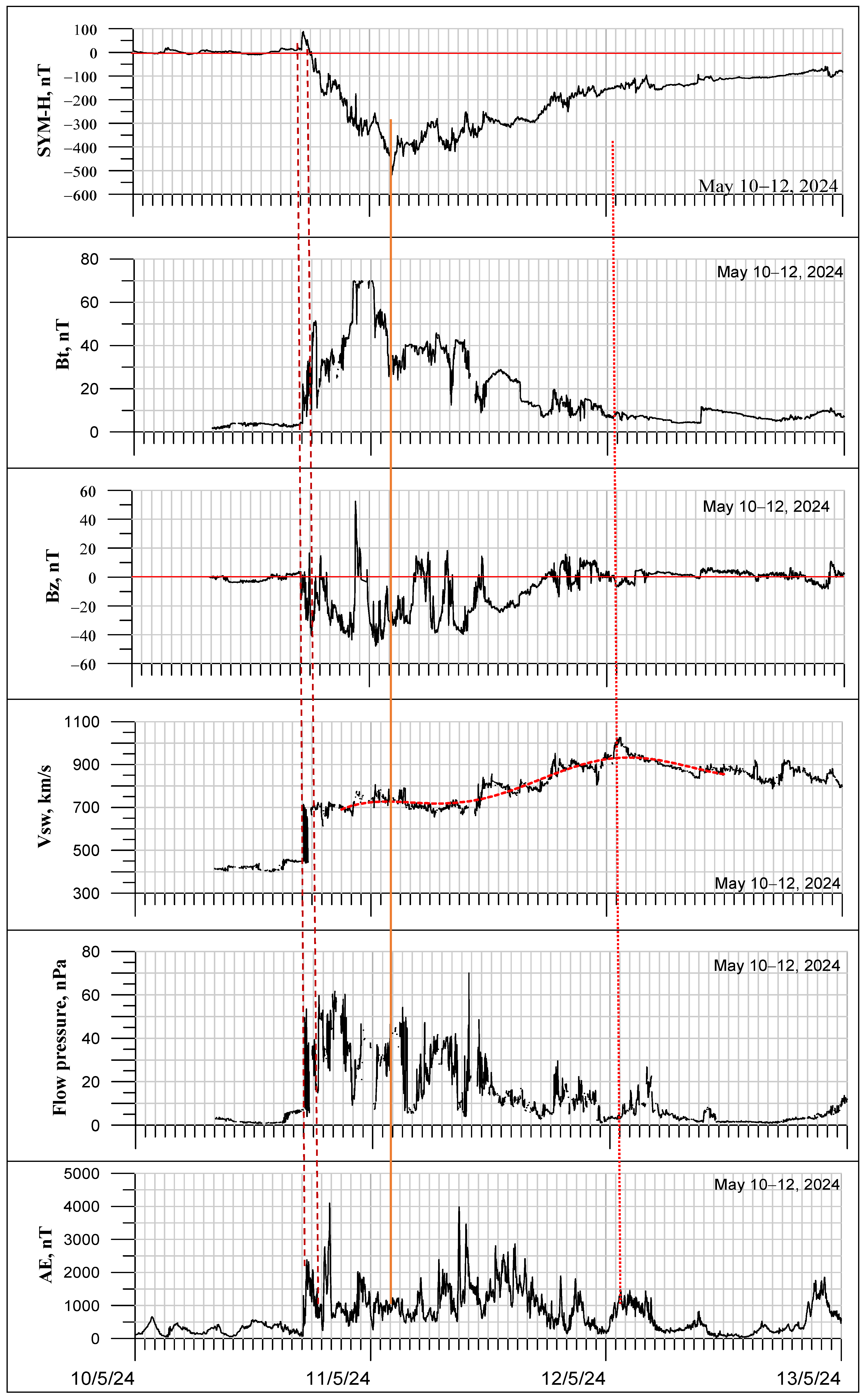
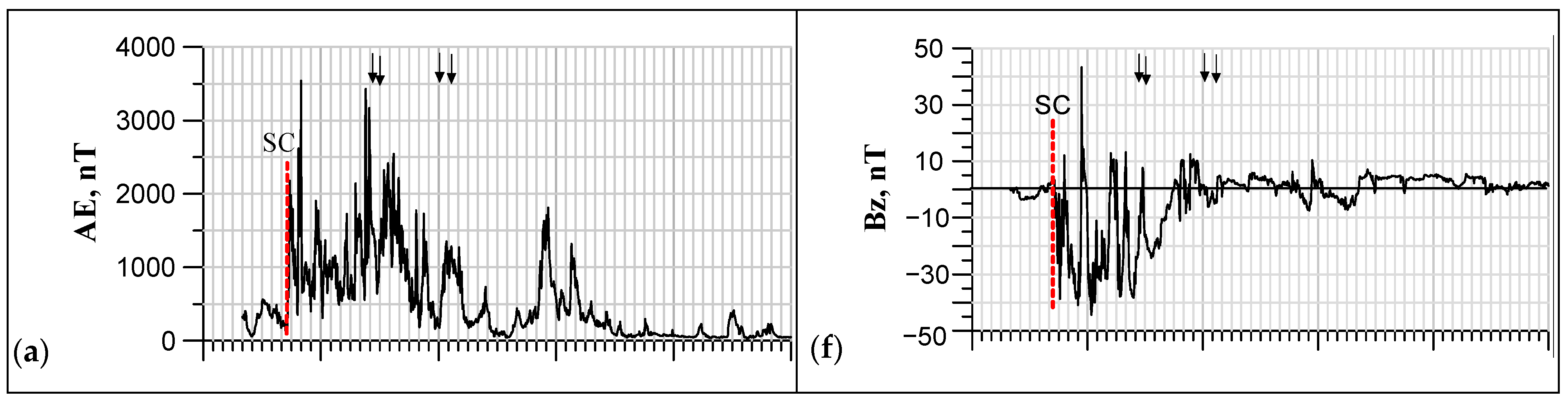
3.1. Solar Wind Parameters and Geomagnetic Indices

Geomagnetic storms are disturbances in the Earth’s magnetosphere resulting from interactions with perturbed solar wind flows. Storm analysis typically distinguishes three phases: (1) the initial phase often marked by a sudden commencement (SC), or storm sudden commencement SSC, or sudden impulse (SI); (2) the main phase, characterized by a significant decrease in geomagnetic indices like Dst or SYM-H; and (3) the recovery phase, during which the indices gradually return toward pre-storm levels [25].
The initial phase of a geomagnetic storm is typically triggered by the arrival of an interplanetary shock wave or the leading edge of a CME impacting the magnetosphere, causing a compression often registered as an SC (if followed by a main phase) or an SI.
In May 2024, NOAA Active Region (AR) 3664, known as NOAA Active Region 13664 according to the NOAA/SWPC region number, was the primary source of solar activity, producing numerous M-class (37) and X-class (9) flares, along with associated CMEs, primarily between 8 and 12 May [11,26]. The X-class flares on 8–9 May likely initiated the CMEs responsible for the subsequent complex interaction with the magnetosphere and the resulting geomagnetic storm on 10–11 May 2024. The initial arrival was marked by a sudden impulse (SI) of 108 nT recorded by the Boulder magnetometer at 16:45 UT on 10 May.
Figure 1 presents UT variations in SYM-H, IMF Bt, IMF Bz, solar wind speed (Vsw), dynamic pressure (Pdyn), and the AE index for 10–12 May 2024. The SYM-H panel indicates an initial positive excursion, associated with the SC, beginning around 17:05 UT on 10 May and lasting approximately 48 min (peak SYM-H: 88 nT at 17:15 UT). The main phase’s development, characterized by a sharp decrease in SYM-H, commenced roughly three hours after the initial impulse. SYM-H then decreased rapidly over approximately 8 h, reaching a minimum value of −518 nT at 02:14 UT on 11 May (indicated by the solid vertical line in Figure 1). Subsequently, SYM-H began to increase, marking the onset of the recovery phase.
During the initial phase (SC), Figure 1 shows a surge in IMF-Bt intensity from ~5 nT to over 30 nT, coinciding with a southward turning of IMF-Bz. Concurrent increases in solar wind speed (from ~450 km/s to ~700 km/s), dynamic pressure, and AE activity were observed, likely associated with the arrival of multiple CMEs [26] carrying strong southward interplanetary magnetic fields. The main phase coincided with elevated IMF-Bt (up to approx. 70 nT), strong IMF-Bz fluctuations (±50 nT) predominantly southward, further increases in solar wind speed and dynamic pressure, and extremely high auroral activity (AE ≈ 3500 nT).
The recovery phase, as depicted in Figure 1, coincided with further intense AE activity, peaking around 09:00 UT on 11 May (AE up to 4000 nT), followed by a gradual decrease toward pre-storm levels by ~06:00 UT on 12 May. During this phase, IMF-Bt decreased, but IMF-Bz remained predominantly southward until ~18:00 UT on 11 May, with intermittent strong southward excursions (down to approx. −30 nT). Solar wind speed continued to increase, peaking near 1000 km/s around 02:00 UT on 12 May. Multiple decreases in SYM-H during the recovery phase coincided with intervals of negative IMF-Bz.
Overall, the analysis suggests the initial storm phase resulted from the increased dynamic pressure upon shock/CME arrival. The main phase developed under conditions of strong IMF magnitude, predominantly southward IMF-Bz, and high dynamic pressure. The total duration of intense interplanetary and geomagnetic activity (from SC until ~02:00 UT on 12 May) coincided with the period of increasing solar wind speed. The storm’s main phase development and duration were closely linked to the presence of strong southward IMF-Bz. Notably, the minimum SYM-H value occurred approximately 1.5 h after the minimum IMF Bz value (−46 nT at 00:41 UT on 11 May).

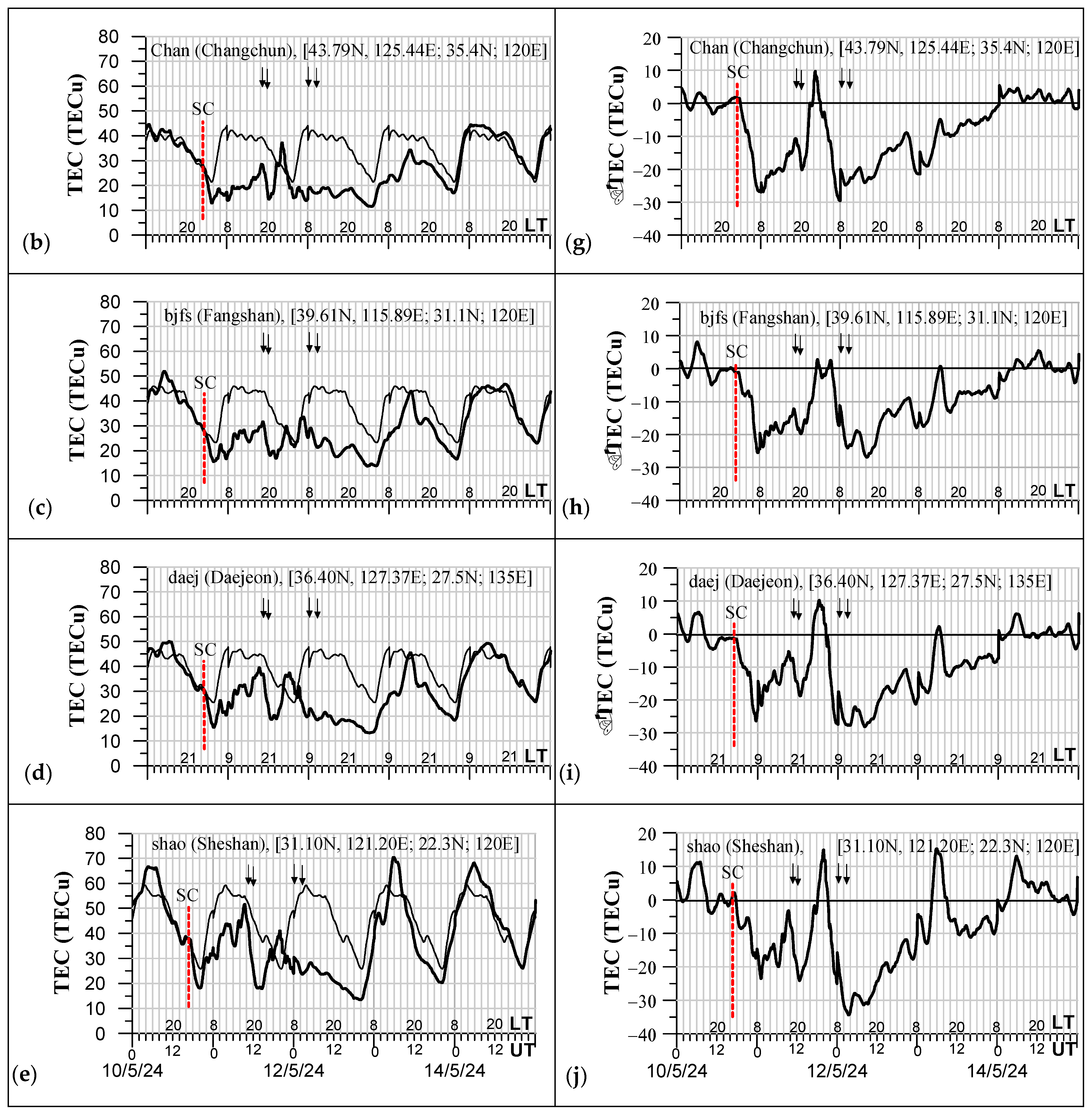
3.2. Observed Effects in the Ionosphere

A detailed discussion of the complex mechanisms driving ionospheric storm responses is beyond the scope of this paper; comprehensive reviews are available in [27,28,29,30,31,32]. However, a brief overview of the mechanism typically responsible for negative ionospheric storm phases, particularly relevant for the Northern Hemisphere in May (summer-like conditions), is warranted.
During geomagnetic disturbances, energy deposition (primarily Joule heating from currents and particle precipitation) in the auroral zones heats the lower thermosphere (100–140 km) [27,29,32]. This heating causes atmospheric upwelling, leading to changes in thermospheric composition at F-region altitudes (~150–600 km). Specifically, the ratio of atomic oxygen density [O] to molecular nitrogen [N2] and oxygen [O2] densities decreases (i.e., with increasing average molecular mass, the [O]/[N2] ratio is reduced) [27]. Since the ion production rate is proportional to [O], and the dominant loss rate for F-region electrons is proportional to [N2] and [O2], a reduced [O]/[N2] ratio leads to decreased electron density (Ne). Additionally, heating generates pressure gradients that drive a storm-induced equatorward circulation. This circulation transports thermospheric air with altered composition (low [O]/[N2]) to lower latitudes, causing the negative ionospheric phase (regions of depleted Ne) to extend equatorward [27,32]. Furthermore, the heated thermospheric gas with reduced [O]/[N2] also has an elevated temperature (T), which increases the chemical loss rate coefficients at F-region altitudes, further contributing to the Ne decrease [32,33]. Thus, negative storm phases are often attributed to the combined effects of reduced [O]/[N2] and increased T [34]. In the summer hemisphere, the prevailing background thermospheric circulation is generally equatorward, which reinforces the storm-induced circulation, facilitating the transport of compositionally disturbed air to mid- and low latitudes [27,32]. Therefore, in the summer hemisphere, negative storm effects can manifest during both daytime and nighttime. Impulsive heating events can initiate traveling atmospheric disturbances (TADs), which manifest in the ionosphere as traveling ionospheric disturbances (TIDs) [28].
Figure 2 shows the TEC variations observed at the Chumish station (CAR region), along with the AE index (Figure 2a) representing geomagnetic activity. The thick solid line shows the observations, while the thin line represents the TEC on the quiet reference day (9 May) for comparison (Figure 2b). The vertical dashed line indicates the SC time. Shortly after the SC (~18:00 UT or 23:00 LT on 10 May, approx. 1 h post-SC), a significant TEC decrease occurred, leading to a prolonged period of depleted TEC, characteristic of a negative ionospheric storm on 11 May (Figure 2b–d). This contrasts with observations in the American sector under similar daytime conditions, where the storm onset featured a sharp TEC increase [12,13]. The deviation from the quiet day (ΔTEC = TEC disturbed − TEC quiet) at Chumish reached a maximum depletion of approximately −37 TECu (Figure 2c) around 02:14 UT (07:14 LT) on 11 May, corresponding to a percentage decrease of about 70% (Figure 2d). This maximum depletion occurred approximately 9 h after the SC and coincided with the minimum SYM-H value. The duration of the most intense part of this negative phase seemed to agree with the duration of southward IMF Bz activity (cf. Figure 1, Bz panel). The total duration of the negative phase, including the recovery, exceeded three days and generally followed the trend of elevated AE activity (Figure 2a). This suggests that the altered thermospheric composition induced by the storm persisted throughout this period. Fluctuations are evident throughout the negative phase (Figure 2c,d), indicating the presence of large-scale irregularities and a disruption of the typical ionospheric structure during both the main and recovery phases. Overall, the ionospheric response observed in Chumysh generally corresponded to the above-described scenario of the development of the negative phase of an ionospheric storm in the summer season, caused by corresponding changes in the composition and circulation of the thermosphere in the middle latitudes.
The ionospheric response to the 10–11 May 2024 geomagnetic storm differed significantly at the Chan GPS station compared to the Chum station, despite their shared latitude. As shown in Figure 3, data from Chan, which lies in the eastern longitudinal sector, reveal this distinct behavior.
At the Chan station, the response was also characterized by a negative storm effect, initiating around the same time (~18:00 UT or 02:00 LT on 10 May, approx. 1 h post-SC). The initial negative phase developed rapidly, reaching its minimum somewhat earlier than at Chumish, around 00:00 UT (08:00 LT) on 11 May. However, during the early recovery phase (afternoon/night LT on 11 May), a brief increase in ΔTEC occurred, followed by a subsequent sharp decrease, forming a distinct secondary negative phase (termed ‘phase 2’) on 12 May. This ‘phase 2’ reached a magnitude comparable to the initial negative phase, but it notably occurred during periods of relatively low AE activity and near-zero or northward IMF-Bz (Figure 1). The total storm duration at Chan also exceeded three days, broadly following the AE activity profile.
The geomagnetic storm on 10–11 May 2024 resulted from the impact of multiple CMEs associated with AR 3664 [27]. Hayakawa et al. [33] estimated subsequent CME arrivals at Earth around 10:32 UT and 11:58 UT on 11 May, and 00:25 UT on 12 May. An additional powerful CME from an X5.8 flare on 11 May was estimated to arrive around 03:16 UT on 12 May [27]. These estimated arrival times are marked by arrows in Figure 3. The TEC response at Chan suggests impacts primarily from the earlier CMEs arriving on 11 May, which coincided with renewed AE intensification (Figure 2a and Figure 3a) and the brief TEC recovery followed by the onset of ‘phase 2’. The impulsive nature of the AE index variations following these arrivals suggests intense energy inputs, possibly generating TADs. The persistence and deepening of the negative phase into 12 May (‘phase 2’), however, occurred under conditions of reduced AE activity and less consistently southward IMF-Bz. This observation suggests that the altered thermospheric composition resulting from the earlier intense energy input may have persisted for over a day in the EAR sector, or that other processes became dominant. The anticipated ionospheric impact from the CME associated with the X5.8 flare (estimated arrival early on 12 May [27]) was not clearly observed as a distinct event in the TEC data, potentially due to a northward or weak embedded magnetic field in that particular CME.
Comparing Figure 2 and Figure 3 clearly shows a significant difference in the ionospheric response between the CAR and EAR sectors at similar latitudes. The primary distinction is the pronounced secondary negative phase (‘phase 2’) observed in the EAR sector (approx. 120° E) during the storm’s recovery phase, which was absent in the CAR sector (approx. 75° E). Additionally, an attempt was made to analyze also the days prior to SC to look for some anomalies during these days and identify ionospheric precursors of geomagnetic storms. The analysis was performed using data from the above-mentioned Chum station and independent TEC observations at Pol2 [42.68 N, 74.69 E] (Bishkek, Kyrgyzstan) for 7–15 May 2024. It was found that, for this event, there were no obvious features in the TEC behavior that could be identified as “precursors”. However, TEC calculations for Pol 2 confirmed that the second phase did not occur for a longitude of 75° E.
To verify this longitudinal difference, TEC variations were analyzed from additional stations (Table 1) within the EAR sector (near the 120° E meridian) spanning different latitudes (Figure 4; due to the lack of data for lower latitudes, it was not possible to consider the latitudinal dependence of TEC changes for the 75° E longitude).
This analysis confirmed that ‘phase 2’ was observed across the latitudinal range studied in the EAR sector (approx. 21° N to 34° N dipole latitude; Figure 4g–j, right panels). The magnitude of ‘phase 2’ appeared to increase toward lower latitudes within this sector, reaching a maximum ΔTEC depletion of approximately −35 TECu (corresponding to approx. −60%) at the Sheshan station (Shao, 21.4° N geographic). As noted, this secondary deep negative phase was not observed at the Chumish station in the CAR region (Figure 4g). Given that ‘phase 2’ occurred during relatively quiescent geomagnetic conditions (low AE, weak/northward Bz), these longitudinal differences are interpreted as potentially reflecting longitudinal variations in storm-induced thermospheric composition changes and/or meridional wind patterns, consistent with the global thermospheric disturbances reported by Evans et al. [11]. Here, it is worth mentioning once again the results of [10,15]. Jain et al. [10], as mentioned above (Section 1), investigated the TEC fluctuations during the geomagnetic storm of 10–11 May 2024, observed in the region of the equatorial ionospheric anomaly (EIA), in Bhopal (23.2° N, 77.4° E, MLAT 14.2° N). The authors analyzed the TEC behavior for 10–13 May 2024 with respect to TEC on the five most quiet days of the month. Observations showed a negative impact of approximately −68.5% deviation in TEC on 11 May 2024, whereas a positive impact was observed with a +61% deviation. The fact is that, according to observations of the Central Asian station Bhopal (meridian 75°E), the second negative phase was also not observed. Moreover, the comparison of diurnal variations in TEC for Chum station (Figure 2b), Bhopal station (Figure 2d in [10]), and other stations of the Indian longitudinal sector (Figure 4 in [10]) shows a noticeable similarity. Kwak et al. [15] investigated the ionospheric response to the geomagnetic storm of 10–11 May 2024 using ionosonde and GNSS receiver data from the East Asian longitude sector where Korea is located. The observations showed a negative ionospheric storm on 11 May (Figure 12 in [15]) and a subsequent decrease in TEC on 12 May (Figure 13 in [15] and references therein). Thus, the results of [10,15] provide additional evidence for the longitudinal difference in the ionospheric response to the geomagnetic storm of 10–11 May 2024 that we discovered.
Additionally, Figure 3b and Figure 4b–e (left panels) show elevated daytime (UT) TEC levels on 11 May across the EAR stations compared to the quiet day. The magnitude of this daytime TEC enhancement on 11 May appeared larger at higher latitudes within this group (e.g., comparing Chan/43.9° N with Shao/21.4° N). This pattern might be indicative of an expansion or intensification of the Equatorial Ionization Anomaly (EIA) structure extending to unusually high mid-latitudes during the main phase in the EAR sector.

4. Conclusions

The ionospheric response to the major geomagnetic storm of 10–11 May 2024 (SYM-H min = −518 nT) was investigated using IONOLAB-TEC data from the Central Asian (CAR) and East Asian (EAR) regions. In the CAR region (Chumish station, ~75° E), a significant negative ionospheric storm phase commenced shortly after the SC (~23:00 LT, 10 May), reaching a maximum TEC depletion of 70% (−37 TECu) around the time of minimum SYM-H on 11 May. The duration of this negative phase correlated with IMF-Bz southward activity, while the overall recovery exceeding three days followed the AE index trend. This behavior is consistent with typical negative storm development driven by thermospheric composition changes.
In contrast, the ionospheric response in the EAR region (~120° E), examined using data from stations spanning 21° N to 34° N dipole latitude, exhibited a significant difference. While an initial negative phase occurred, a distinct, secondary deep negative phase (“phase 2”) developed on 12 May. This “phase 2” reached comparable or greater intensity than the initial depletion (−35 TECu or ~−60% at lower latitudes) but occurred during a period of reduced geomagnetic activity (low AE, weak/northward IMF-Bz). This secondary depletion was not observed in the CAR sector. Additionally, evidence suggested a possible expansion of the EIA to higher mid-latitudes in the EAR sector during the main phase on 11 May.
This comparative analysis highlights the significant longitudinal variability in the ionospheric response to a major geomagnetic storm. The pronounced difference, particularly the emergence of “phase 2” in the EAR sector during the recovery phase under quiescent conditions, suggests substantial longitudinal variations in the storm-induced thermospheric state (composition and/or dynamics) between the CAR and EAR sectors.

Author Contributions

G.G.: research model, methodology, original draft preparation; F.A.: writing Section 2, review and editing; Y.L. and M.Z.: investigation, visualization. All authors have read and agreed to the published version of the manuscript.

Funding

This research was funded by the Science Committee of the Ministry of Science and Higher Education of the Republic of Kazakhstan, grant number BR20280979 “Comprehensive study of the impact of solar disturbance sources on the state of near-Earth space”.

Institutional Review Board Statement

Not applicable.

Informed Consent Statement

Not applicable.

Data Availability Statement

The TEC data used in this study were obtained from the publicly accessible IONOLAB service (http://www.ionolab.org). Solar wind and geomagnetic indices were obtained from the NASA/GSFC OMNIWeb database (https://omniweb.gsfc.nasa.gov/form/omni_min.html, accessed on 7 July 2025). Further derived data presented in this study are available upon request from the corresponding author.

Conflicts of Interest

The authors declare no conflicts of interest.

References

  1. Gopalswamy, N.; Yashiro, S.; Michalek, G.; Xie, H.; Lepping, R.P.; Howard, R.A. Solar source of the largest geomagnetic storm of cycle 23. Geophys. Res. Lett. 2005, 32, L12S09. [Google Scholar] [CrossRef]
  2. Daglis, I.A.; Chang, L.C.; Dasso, S.; Gopalswamy, N.; Khabarova, O.V.; Kilpua, E.; Lopez, R.; Marsh, D.; Matthes, K.; Nandy, D.; et al. Predictability of variable solar–terrestrial coupling. Ann. Geophys. 2021, 39, 1013–1035. [Google Scholar] [CrossRef]
  3. Lam, H.-L.; Boteler, D.H.; Trichtchenko, L. Case studies of space weather events from their launching on the Sun to their impacts on power systems on the Earth. Ann. Geophys. 2002, 20, 1073–1079. [Google Scholar] [CrossRef]
  4. Lanzerotti, L.J. Space weather effects on technologies. In Space Weather; Song, P., Singer, H.J., Siscoe, G.L., Eds.; Geophysical Monograph Series 125; American Geophysical Union: Washington, DC, USA, 2001; pp. 11–22. [Google Scholar] [CrossRef]
  5. Basu, S.; Basu, S.; Makela, J.J.; MacKenzie, E.; Doherty, P.; Wright, J.W.; Rich, F.; Keskinen, M.J.; Sheehan, R.E.; Coster, A.J. Large magnetic storm-induced nighttime ionospheric flows at midlatitudes and their impacts on GPS-based navigation systems. J. Geophys. Res. 2008, 113, A00A06. [Google Scholar] [CrossRef]
  6. Afraimovich, E.L.; Demyanov, V.V.; Kondakova, T.N. Degradation of GPS performance in geomagnetically disturbed conditions. GPS Solut. 2003, 7, 109–119. [Google Scholar] [CrossRef]
  7. Bolduc, L. GIC observations and studies in the Hydro-Québec power system. J. Atmos. Sol.-Terr. Phys. 2002, 64, 1793–1802. [Google Scholar] [CrossRef]
  8. Gaunt, C.T.; Coetzee, G. Transformer failures in regions incorrectly considered to have low GIC-risk. In Proceedings of the IEEE Lausanne Power Tech, Lausanne, Switzerland, 1–5 July 2007; pp. 807–812. [Google Scholar] [CrossRef]
  9. Dang, T.; Li, X.; Luo, B.; Li, R.; Zhang, B.; Pham, K.; Ren, D.; Chen, X.; Lei, J.; Wang, Y. Unveiling the Space Weather during the Starlink Satellites Destruction Event on 4 February 2022. Space Weather 2022, 20, e2022SW003152. [Google Scholar] [CrossRef]
  10. Lee, W.K.; Kil, H.; Choi, B.K.; Hong, J.; Jeong, S.H.; Kim, S.; Kim, J.H.; Sohn, D.H.; Roh, K.M.; Yoo, S.M.; et al. Ionospheric Responses to the May 2024 G5 Geomagnetic Storm Over Korea, Captured by the Korea Astronomy and Space Science Institute (KASI) Near Real-Time Ionospheric Monitoring System. J. Space Technol. Appl. 2024, 4, 210–219. [Google Scholar] [CrossRef]
  11. Evans, J.S.; Correira, J.; Lumpe, J.D.; Eastes, R.W.; Gan, Q.; Laskar, F.I.; Aryal, S.; Wang, W.; Burns, A.G.; Beland, S.; et al. GOLD observations of the thermospheric response to the 10–12 May 2024 Gannon superstorm. Geophys. Res. Lett. 2024, 51, e2024GL110506. [Google Scholar] [CrossRef]
  12. Tulasi Ram, S.; Veenadhari, B.; Dimri, A.P.; Bulusu, J.; Bagiya, M.; Gurubaran, S.; Parihar, N.; Remya, B.; Seemala, G.; Singh, R.; et al. Super-intense geomagnetic storm on 10–11 May 2024: Possible mechanisms and impacts. Space Weather 2024, 22, e2024SW004121. [Google Scholar] [CrossRef]
  13. Singh, R.; Scipion, D.E.; Kuyeng, K.; Condor, P.; De La Jara, C.; Velasquez, J.P.; Flores, R.; Ivan, E.; Souza, J.R.; Migliozzi, M. Ionospheric disturbances observed over the Peruvian sector during the Mother’s Day Storm (G5-level) on 10–12 May 2024. J. Geophys. Res. Space Phys. 2024, 129, e2024JA033003. [Google Scholar] [CrossRef]
  14. Bojilova, R.; Mukhtarov, P.; Pancheva, D. Global Ionospheric Response During Extreme Geomagnetic Storm in May 2024. Remote Sens. 2024, 16, 4046. [Google Scholar] [CrossRef]
  15. Kwak, Y.-S.; Lee, C.; Lee, D.-Y.; Ham, Y.-B.; Kim, Y.H.; Lee, J.J.; Kim, J.-H.; Kim, S.; Miyashita, Y.; Yang, T.; et al. Observational overview of the May 2024 g5-level geo-magnetic storm: From solar eruptions to terrestrial consequences. J. Astron. Space Sci. 2024, 41, 171–194. [Google Scholar] [CrossRef]
  16. Jain, A.; Trivedi, R.; Jain, S.; Choudhary, R.K. Effects of the Super Intense Geomagnetic Storm on 10-11 May, 2024 on Total Electron Content at Bhopal. Adv. Space Res. 2025, 75, 953–965. [Google Scholar] [CrossRef]
  17. Pierrard, V.; Verhulst, T.G.W.; Chevalier, J.-M.; Bergeot, N.; Winant, A. Effects of the Geomagnetic Superstorms of 10–11 May 2024 and 7–11 October 2024 on the Ionosphere and Plasmasphere. Atmosphere 2025, 16, 299. [Google Scholar] [CrossRef]
  18. Karan, D.K.; Martinis, C.R.; Daniell, R.E.; Eastes, R.W.; Wang, W.; McClintock, W.E.; Michell, R.G.; England, S. GOLD observations of the merging of the Southern Crest of the equatorial ionization anomaly and aurora during the 10 and 11 May 2024 Mother’s Day super geomagnetic storm. Geophys. Res. Lett. 2024, 51, e2024GL110622. [Google Scholar] [CrossRef]
  19. Guo, X.; Zhao, B.; Yu, T.; Hao, H.; Sun, W.; Wang, G.; He, M.; Mao, T.; Li, G.; Ren, Z. East–west difference in the ionospheric response during the recovery phase of May 2024 super geomagnetic storm over the East Asian. J. Geophys. Res. Space Phys. 2024, 129, e2024JA033170. [Google Scholar] [CrossRef]
  20. Arikan, F.; Erol, C.B.; Arikan, O. Regularized estimation of vertical total electron content from Global Positioning System data. J. Geophys. Res. Space Phys. 2003, 108, 1469. [Google Scholar] [CrossRef]
  21. Arikan, F.; Erol, C.B.; Arikan, O. Regularized estimation of vertical total electron content from GPS data for a desired time period. Radio Sci. 2004, 39, RS6010. [Google Scholar] [CrossRef]
  22. Nayir, H.; Arikan, F.; Arikan, O.; Erol, C.B. Total electron content estimation with Reg-Est. J. Geophys. Res. Space Phys. 2007, 112, A11312. [Google Scholar] [CrossRef]
  23. Arikan, F.; Nayir, H.; Sezen, U.; Arikan, O. Estimation of single station interfrequency receiver bias using GPS-TEC. Radio Sci. 2008, 43, RS4013. [Google Scholar] [CrossRef]
  24. Sezen, U.; Arikan, F.; Arikan, O.; Ugurlu, O.; Sadeghimorad, A. Online, automatic, near-real time estimation of GPS-TEC: IONOLAB-TEC. Space Weather 2013, 11, 297–305. [Google Scholar] [CrossRef]
  25. Loewe, C.A.; Prölss, G.W. Classification and mean behavior of magnetic storms. J. Geophys. Res. Space Phys. 1997, 102, 14209–14213. [Google Scholar] [CrossRef]
  26. Hayakawa, H.; Ebihara, Y.; Mishev, A.; Koldobskiy, S.; Kusano, K.; Isobe, H.; Bechet, S.; Yashiro, S.; Iwai, K.; Shinbori, A.; et al. The Solar and Geomagnetic Storms in 2024 May: A Flash Data Report. Astrophys. J. 2025, 979, 49. [Google Scholar] [CrossRef]
  27. Prölss, G. Ionospheric F-region storms. In Handbook of Atmospheric Electrodynamics; Volland, H., Ed.; CRC Press: Boca Raton, FL, USA, 1995; Volume 2, pp. 195–248. [Google Scholar] [CrossRef]
  28. Buonsanto, M.J. Ionospheric Storms—A Review. Space Sci. Rev. 1999, 88, 563–601. [Google Scholar] [CrossRef]
  29. Danilov, A.D.; Lastovicka, J. Effects of Geomagnetic Storms on the Ionosphere and Atmosphere. Int. J. Geomagn. Aeron. 2001, 2, 209–219. [Google Scholar]
  30. Mendillo, M. Storms in the ionosphere: Patterns and processes for total electron content. Rev. Geophys. 2006, 44, RG4001. [Google Scholar] [CrossRef]
  31. Prölss, G.W. Ionospheric Storms at Mid-Latitude: A Short Review. In Midlatitude Ionospheric Dynamics and Disturbances; Kintner, P.M., Jr., Coster, A.J., Fuller-Rowell, T., Mannucci, A.J., Mendillo, M., Heelis, R., Eds.; Geophysical Monograph Series 181; American Geophysical Union: Washington, DC, USA, 2008; pp. 13–21. [Google Scholar] [CrossRef]
  32. Danilov, A.D. Ionospheric F-region response to geomagnetic disturbances. Adv. Space Res. 2013, 52, 343–366. [Google Scholar] [CrossRef]
  33. Mikhailov, A.V.; Foster, J.C. Daytime thermosphere above Millstone Hill during severe geomagnetic storms. J. Geophys. Res. 1997, 102, 17275–17282. [Google Scholar] [CrossRef]
  34. Mikhailov, A.V.; Förster, M. Day-to-day thermosphere parameter variation as deduced from Millstone Hill incoherent scatter radar observations during March 16–22, 1990 magnetic storm period. Ann. Geophys. 1997, 15, 1429–1438. [Google Scholar] [CrossRef]
Figure 1. UT variations in SYM-H, IMF-Bt, IMF-Bz, solar wind speed (Vsw), dynamic pressure (Pdyn), and the AE index for 10–12 May 2024.
Atmosphere 16 00854 g001
Figure 2. UT variations in the (a) AE index, (b) TEC, (c) ΔTEC (in TECu), and (d) ΔTEC (in %) observed at Chumish station during 10–14 May 2024. LT times are indicated above the x-axis; the corresponding UT times are indicated below the x-axis. Vertical dotted lines mark the SC time. The thin black line in Figure 2b represents the quiet-day behavior.
Atmosphere 16 00854 g002
Figure 3. UT variations in the (a) AE index, (b) TEC, (c) ΔTEC (in TECu), and (d) ΔTEC (in %) observed at Changchun station during 10–14 May 2024. LT times are indicated above the x-axis; the corresponding UT times are indicated below the x-axis. Vertical dotted lines mark the SC time. The thin black line in Figure 3b represents the quiet-day behavior.
Atmosphere 16 00854 g003
Figure 4. UT variations in the (a) AE index and (f) IMF-Bz component, as well as (be) TEC (left panels) and (gj) ΔTEC (right panels), both in TECu, during 10–14 May 2024 for GPS stations: (b,g) Chan, (c,h) Bjfs, (d,i) Daej, and (e,j) Shao. UT times are below the x-axis; corresponding LT (UTC+5 for Chumish, UTC+8 for others) are above the x-axis. Vertical dotted lines mark the SC time.
Atmosphere 16 00854 g004aAtmosphere 16 00854 g004b
Table 1. GPS stations used in this study.
Station Code
(Station Name, Location)
Geog. Lat. (°N)Geog. Long. (°E)Geom. Lat. (°N)Time Zone (°E)Region
Chum
(Chumish, Kazakhstan)
42.9974.7535.3UTC+5CAR
Chan
(Changchun, China)
43.79125.4435.4UTC+8EAR
Bjfs
(Fangshan, China)
39.61115.8931.1UTC+8EAR
Daej
(Daejeon, Korea)
36.40127.3727.5UTC+9EAR
Shao
(Sheshan, China)
31.10121.2022.3UTC+8EAR
Disclaimer/Publisher’s Note: The statements, opinions and data contained in all publications are solely those of the individual author(s) and contributor(s) and not of MDPI and/or the editor(s). MDPI and/or the editor(s) disclaim responsibility for any injury to people or property resulting from any ideas, methods, instructions or products referred to in the content.

