Performance of Low-Cost Air Temperature Sensors and Applied Calibration Techniques—A Systematic Review

Abstract

Low-cost air temperature sensors are an emerging theme in environmental monitoring. These sensors offer the advantage of making microclimate monitoring feasible due to their affordability. However, they are limited by the quality of the data they provide; in many cases, they have been reported to have presented errors in the sensor readings. These errors have been shown to improve after calibration was applied. The lack of a comprehensive understanding of the available calibration techniques, models, and sensor types has led to studies presenting heterogeneity in models and techniques alongside different performance metrics. To address this gap, this study conducted a systematic review following the PRISMA guidelines, reviewing studies from 2015 to 2024 across the databases Web of Science and Scopus, alongside the search engine Google Scholar. The aim was to identify the calibration techniques and models, the commercially available low-cost air temperature sensors used, the performance metrics utilised, and the calibration settings. The findings presented three main categories of calibration models utilised in the collected studies: linear, polynomial, and machine learning. Twenty-two commercially available low-cost sensors were identified, with the DHT22 sensor being the most utilised. Indoor settings were identified as the most preferred for conducting calibrations. Key challenges included limitations in reported results for calibration by the studies, the use of different performance metrics across studies, insufficient studies conducting calibration, and the diversity in sensor types utilised.

1. Introduction

Agriculture plays a crucial role in modern society, forming the backbone of the global food industry and being a key factor for the global economy [1], with the rapid growth of population leading to an over-reliance on conventional farming practices in order to meet demand [2]. However, the implementation of these farming practices, such as conventional tillage, often poses significant challenges to the environment, such as climate change, soil degradation, and CO₂ emissions [3,4,5]. The urgent need to shift to more sustainable and still-productive systems of farming instigated the development of precision agriculture (PA). The International Society of Precision Agriculture (ISPA) defines PA as a management strategy that involves gathering, processing, and analysing data over time and across locations for individual plants and animals [6].

Data acquisition is one of the most essential components of PA; in particular, capturing meteorological data is crucial for agricultural practices [7,8]. Among these data, air temperature stands out as a vital parameter, influencing not only crop yields but also livestock productivity and the overall stability of agricultural ecosystems. It is often leveraged in crop yield production models, serving an essential role [9,10,11]. In crop production, a fluctuation of ±2 °C from the mean seasonal temperatures during the wheat growing season could lead to significant grain yield losses, potentially reaching up to 50% [12,13]. From the perspective of livestock production, heat stress resulting from temperature fluctuations has been shown to reduce milk yield in dairy cows by approximately −0.17 kg/°C to −0.38 kg/°C [14,15]. This underscores the importance of precise air temperature monitoring, particularly from a microclimatic perspective.

There are two main types of temperature sensors: contact and non-contact sensors. Non-contact sensors, such as infrared devices, utilise radiated energy, while contact sensors include thermistors, thermocouples, resistance temperature detectors (RTDs), and semiconductor sensors [16]. Thermistors are resistors made from ceramic materials, such as oxides of nickel, manganese, or cobalt, and exhibit significant changes in resistance with temperature [17,18]. Thermocouples consist of two metals joined together at two junctions: one measures the temperature (hot), while the other connects to a reference body (cold). RTDs, such as platinum resistance thermometers (PRTs), use pure metals with resistance proportional to temperature changes. Semiconductor sensors made from silicon measure temperature by detecting the voltage drop across a diode [16,19,20].

The systems currently available for temperature monitoring, including fixed meteorological stations, mobile meteorological stations, and satellite-based systems, face limitations. Fixed meteorological stations, as their name suggests, are situated at a single point in a specific location. These stations are equipped with advanced thermometers that provide accurate air temperature readings; however, they are limited in terms of spatial coverage and entail high deployment costs [21,22]. Mobile meteorological stations provide an advantage over fixed stations by offering data from multiple spatial points within a region, thus enhancing coverage. However, they have the limitation of not delivering data over a continuous time series and necessitate relocation each time [22]. Another method for monitoring temperature is the use of remote sensing tools, such as satellites. These systems utilize infrared radiation to monitor temperature. In the absence of dense networks of fixed and mobile meteorological stations, these satellites can provide spatial-temporal distribution, which can be used as a parameter to complement the meteorological stations. However, their feasibility is limited in indoor settings and under cloud cover [23].

The integration of wireless sensor networks (WSNs) that utilize low-cost air temperature sensors into precision agriculture offers a promising solution to complement current monitoring systems. WSNs are the major drivers in precision agriculture; they are composed of compact micro-sensors with wireless communication capabilities, consisting of hundreds or even thousands of these micro-sensors [7,8]. The term “low-cost sensors” has been interpreted in many ways by different researchers [24]. These sensors are typically small and low-cost; thus, they can be deployed in harsh environments like an agricultural field without risk of significant losses due to sensor damage. These sensors have enabled the feasibility of monitoring micro-climates since they can be deployed in large numbers. Most of these sensors fall in the category of thermistors and semiconductors. They are typically ten or more times less expensive than conventional meteorological sensors, which are generally expensive due to their complexity and require a lot of maintenance [25]. These sensors, however, face limitations in terms of data reliability, as numerous studies have pointed out [26]. Calibration has been recognised as a crucial step in addressing concerns of reliability.

These sensors have been shown to provide accurate data with scientifically correct calibration methods. Calibration entails comparing the readings of the sensor to a reference instrument in either a controlled setting, such as a laboratory, or in a co-location setting either indoors or outdoors to assess sensor performance in its intended place of application [24,27]. Calibration of low-cost sensors can be viewed primarily in two ways: by comparison with high-end reference instruments or using low-cost, less expensive calibration methods. The choice of calibration method is subjective and depend on whether the individual tends to be a maximiser or satisfier. A maximiser seeks the best possible outcomes, often leveraging the use of state-of-the-art instruments for sensor calibration. They are usually resource-intensive and can sometimes be unfeasible without proper access. In contrast, a satisfier’s objective is to achieve reliable calibration results at a lower cost, prioritising cost-efficiency and simplicity in their calibration procedures [28].

Despite the numerous studies on the calibration of low-cost air temperature sensors, a limited number of studies have conducted calibration in field settings. Additionally, several prior reviews have covered the calibration of low-cost sensors in a broader environmental area. Karagulian et al. (2019) reviewed the performance of low-cost air quality sensors, highlighting the need for more unified calibration approaches, though their study primarily focused on pollution sensors, with minimal reference to temperature measurement [29]. Chojer et al. (2020) similarly emphasized the general lack of standardized reporting across low-cost sensor calibration studies, additionally noting that most studies lack calibration results, limiting their comparability [26]. However, there is a lack of comprehensive reviews to date primarily focusing on the calibration of low-cost air temperature sensors, underscoring the need for a focused and rigorous study. To address these challenges, this study conducted a systematic review of the present methods and models of calibration, the types of low-cost temperature sensors used, and their advantages and limitations. This review followed the 2020 PRISMA guidelines for critical analysis of the existing literature.

The objectives of this study are the following:

• Identifying and analysing the calibration models and their calibration methods to understand the best model performance.
• To understand which type of low-cost sensor is the most used in temperature measurement.
• To analyse the performance of sensors under various influencing factors.
• Identify the settings where these types of sensors are most utilised, whether in outdoor or indoor environments. While it was aimed to find studies calibrated at temperatures ranging from −10 °C to 40 °C, which are typical of agricultural conditions, we adjusted our focus to include more studies due to the limited number of papers in this range, particularly in the agricultural context.
• Identify the challenges that current calibration models and methods pose to researchers in this field.

2. Methodology

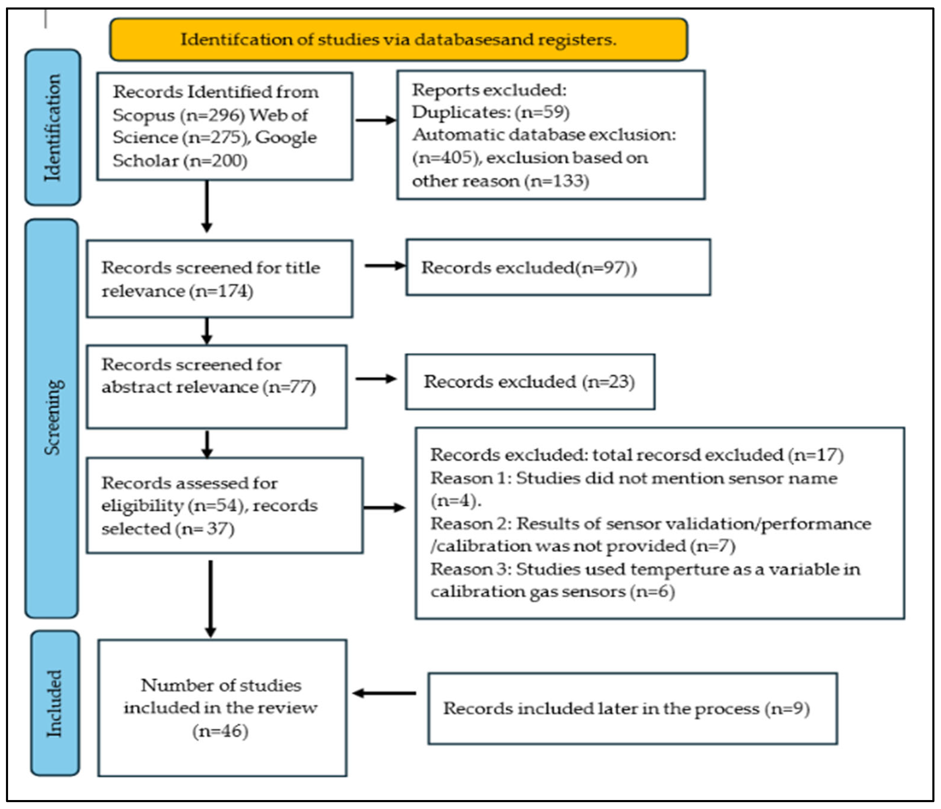
This study conducted a systematic literature review following the Preferred Reporting Items for Systematic Reviews and Meta-Analyses (PRISMA) guidelines to ensure transparency and minimize bias in the studies collected [30,31] (Figure 1).

• Eligibility Criteria

This review utilized specific criteria for selecting studies for inclusion and exclusion. These criteria outline the types of scientific papers that were deemed eligible for inclusion in this review.

➢

Studies eligible for inclusion were published journal papers and conference papers; these studies were required to be full-text published papers. Restrictions were not placed on the status of peer-reviewed studies.

➢

Studies eligible for inclusion had to focus on sensor calibration, specifically testing low-cost air temperature sensors (LCSs).

➢

“Low-cost sensors” were those placed in the range of less than USD 50. This value was agreed upon due to variation in global prices due to differences in tax policies, material costs, and sensor availability, with costs ranging from USD 5 in some countries to USD 20 in others. The sensors used must be compatible with low-cost microcontrollers such as Arduino (https://www.arduino.cc, accessed 15 October 2024) or Raspberry Pi (https://www.raspberrypi.com, accessed 15 October 2024). No restrictions were placed for the type of model used; any board from these platforms were considered eligible.

➢

Despite no formal restriction on the publication dates, the focus on sensors compatible with microcontrollers such as Arduino and Raspberry Pi introduced a timeline boundary, since these microcontrollers were introduced in the period between 2005 and 2012.

➢

The selected studies’ methodology must detail the sensor calibration process. In the case of limited calibration-focused studies, additional studies that utilised calibration models for sensor validation were eligible for inclusion to reduce bias resulting from the number of studies.

➢

The studies were required to include details on the performance metrics utilised for sensor and calibration assessment.

➢

Studies that failed to specify the type of low-cost sensor utilised, lacked performance metrics, did not specifically mention the sue of low-cost air temperature sensors, or were not published as full-text studies were excluded.

➢

There was no restriction on the settings where the experiments were conducted.

➢

In terms of language used in the studies, no restrictions were placed, since most of the calibration data were in numerical figures and graphs.

• Information Source

The selection process lasted from August 2024 to November 2024. The studies were sourced from Google Scholar, Scopus, and Web of Science. To ensure literature saturation, we sourced studies from the reference lists of the eligible studies.

• Search strategy

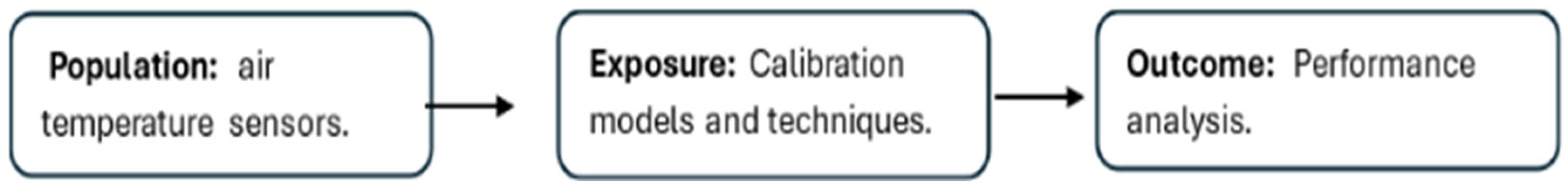
The search strategy was developed using the Population Exposure Outcome (PEO) framework (Figure 1).

Using this framework, the keywords were categorised into three categories:

➢

Population: Described the types of sensors leading to the selection of keywords such as “Low-cost”, “Temperature sensors”, “Arduino”, “Raspberry Pi*”, and “Air temperature”.

➢

Exposure/Intervention: Implied interventions placed on the experimented sensor leading to the selection of keywords such as “Sensor calibration”, “Sensor correction”, and “Calibrate*”.

➢

Outcome: Entailed the expected outcomes of the interventions applied on the sensors in terms of performance metric. This led to selection of keywords such as “Calibration performance”, “Reliability of sensors”, “Sensor accuracy” “sensor error”, and “Calibration error”.

These keywords were used for the literature search on Scopus and Web of Science. Boolean operators such as “AND” and “OR” were applied on Web of Science and Scopus, and additional operators like “AND NOT” were used to exclude unrelated studies. This exclusion was necessary because the initial search returned a large number of studies on low-cost pollution sensors such as particulate matter (PM), CO₂, and NO₂ sensors, rather than low-cost air temperature sensors. This led to the formulation of search strings such as the following:

➢

“Calibration” AND “air temperature” AND “sensors” AND NOT “CO₂ concentration” AND NOT “Pm2.5/Pm10”.

➢

“Calibration performance” “AND” “air temperature sensors”.

➢

“Accuracy” AND “Calibration” AND “Low-cost” AND “Temperature sensors” AND “Arduino” OR “Raspberry Pi*”.

➢

“Temperature calibrations”.

➢

“Low-cost” AND “Calibration” AND “air temperature sensors” AND “arduino” OR “Raspberry Pi”.

Additionally, key sentences without Boolean operators were utilised on Google Scholar and Web of Science; these are “Calibration of low-cost air temperature sensor”, “Performance of low-cost air temperature sensor”, “air temperature sensor calibration techniques”, “Reliability of low-cost air temperature sensors”, “Comparative analysis of low cost air temperature sensors”, and “Low cost air temperature sensors performance evaluation for air temperature measurement”. To enhance the process, the exclusion and inclusion filters available on Scopus and Web of Science were utilised. On Web of Science, keywords like “particulate matter”, “nitrogen dioxide”, “particulate matter pm”, “soil water content”, “pollution measurement”, and any other keywords related to pollution and gas sensing were excluded using the “EXCLUDE” option on the database. On Scopus, the option of “Limit to” OR “Exclude” was used, limiting the studies to articles, conference papers, and reviews only. The option was also used to limit and exclude keywords according to our inclusion and exclusion criteria.

• Selection Process

The selection process yielded an initial 296 studies on Scopus and 275 studies on Web of Science; after applying the filters mentioned, the final studies for each database were 87 studies and 79 studies, respectively (see Figure 2). These studies were assessed manually for title relevance, yielding 35 and 17 studies for Scopus and Web of Science, respectively. For each key sentence, the first 50 studies were assessed for title relevance on Google Scholar during each search round. The abstract of each study was evaluated, following the previous inclusion criteria, and the selected studies were added to a shared Google Sheet. This process resulted in a final number of 46 studies, including 22 low-cost sensors (see Tables 1 and 2). Of these 46 studies, nine were sourced from references in sections from the selected studies. Among the collected studies, five were published in Indonesian and were translated into English using the Microsoft Word feature for translating documents [32,33,34,35,36]. Three independent reviewers conducted the screening process. While efforts were made to document all exclusions, some discrepancies arose in tracking the exact number of excluded studies. Thus, the data provided are an estimate within a reasonable confidence range. This limitation was addressed by cross-checking exclusion criteria and ensuring consistency in the selection process.

• Data collection

The selected studies were organized into the following categories:

➢

Sensor types, which entailed how the sensors perform to measure temperature, whether using a thermistor or a semiconductor.

➢

Calibration model or the validation analysis used to compare or calibrate the sensors.

➢

In the cases of direct approach, with no use of any statistical models, this was classified under direct comparison, along with studies that did not give any information on the models used.

➢

Environmental settings of the studies where calibration was carried out. This was categorised into indoors or controlled environments and uncontrolled environments or outdoors.

➢

Performance accuracies: This was presented in terms of errors such as RMSE (root mean square error), MSE (mean square error), mean error, MAE (mean absolute error), standard deviation, and uncertainty. The RMSE shows the average of the largest possible errors to be expected from the sensor, or the models as compared to the reference, with magnitude but without direction. MAE gives an average of the errors without direction. The mean error will show the average of the errors with direction; it gives a hint that the system may experience bias. Additional performance metrics were included from the studies on the calibration model performance; this included the R² (coefficient of determination) values, which show how well the reference sensor and the calibrated sensor agree.

➢

Additional details like the reference sensor, duration of calibration, and calibration models used (linear regression, polynomial regression, and machine learning algorithms) were collected.

• Study risk of bias assessment

While no formal tool or software was used to assess for bias, a structured review process was established to minimise bias in the selected studies. These measures were as follows:

➢

The data collection process was conducted on a shared Excel file and a Google Sheet document to ensure transparency among reviewers.

➢

The reviewers would occasionally check for duplicated studies within the Excel file or Google Sheet and flag them for exclusion. Additionally, details on journal and authors were included in the studies. This enabled the identification of similar research published under different titles. The more detailed or original of the duplicates were retained for inclusion. These studies were labelled as high risk.

➢

For data transparency within the collected studies, reviewers would passively read the sections of the studies. Studies that lacked numerical results or presented unsupported claims in the discussion or conclusion sections—without corresponding data in the results—were excluded (also labelled as high risk). Preference was given to studies that clearly reported performance metrics (e.g., RMSE, MAE, or R²) and calibration models.

However, due to the limited number of studies, those with a moderate risk of bias were acceptable. This was in studies that presented calibration or validation methodologies but in shallow sense. Additionally, five studies were translated from Indonesian to English using Microsoft Word 365’s built in translator (Microsoft^® Word for Microsoft 365 MSO (Version 2505 Build 16.0.18827.20102) 64 bit)). While these studies may introduce bias due to translation risks, details on the calibration that were presented numerically were checked by one of the experienced reviewers, Dr. István Mihály Kulmány, who was experienced in sensor calibration [4]. An additional translation test was conducted using Google Translate, where we selected random paragraphs from the texts and compared the translation from Google Translate with the Microsoft translation. The results showed minor phrasal differences, but the meaning of each paragraph was the same in both. These studies were accepted for inclusion since the data presented could be followed.

• Synthesis Method

The studies collected were synthesized into groups for calibration models, sensor types, and performance across sensor types and across calibration models. Studies that were grouped into calibration models provided details on the type of sensor utilised and the performance of the sensor before calibration and after calibration. Additionally, due to the limited number of calibration-focused studies utilising similar models for sensor validation were included in the synthesis described in Section 3.1. For sensor types and performance evaluation, studies that also applied direct comparison were included for comparison in sensor performance across varies temperatures.

The findings of the synthesis will be presented in Section 3 and an elaboration of the results presented in Section 4.

3. Results

This systematic review synthesizes findings from 46 studies published between 2015 and 2024, sourced from Google Scholar, Web of Science, and Scopus. The studies were distributed across six continents and involved 22 different types of low-cost temperature sensors (see Figure 3 and Figure 4), highlighting the global research interest in low-cost environmental monitoring tools. A notable concentration of research was observed in Indonesia, with 14 studies contributing to the field (see Figure 3). The findings are organised thematically by sensor types, calibration models, deployment settings, and study durations in the following sections.

3.1. Calibration Models

Of the 46 studies included in this review, 20 studies utilized calibration or validation models for accuracy improvements or for validation of the low-cost air temperature sensors, while 26 studies either relied on direct comparison without the application of calibration models or provided insufficient information regarding the models used for calibration or validation. A summary of the performance of the models alongside the sensor types used is provided in Table 1.

The models employed were grouped into four categories, i.e., linear regression, polynomial regression, machine learning models, and direct comparison or non-model approaches (no models were applied, and just a direct comparison was conducted) (Figure 5).

3.1.1. Linear Regression Models

Linear regression was the most utilised model, applied in 17 of the studies in this review. The model served as a calibration model or validation tool for sensor performance. Several studies noted performance improvements after calibration using linear models [37,38,39]. For instance, the mean error of the DS18B20 (Analog Devices, Wilmington, MA, USA) sensor calibrated in an oil medium was reported to have reduced from 3% to 0.85%, with an increase in R² value from 0.989 to 0.994, and the standard error decreased by 48.25% in the temperature range of 23–30 °C [37]. Further evidence of improvements was reported in the calibration of the BME280 [38]. Improvements were noted in R² when both single and multivariate linear regression were used, obtaining an R² of 0.9939 and 0.9929, respectively. This was an improvement from the original R² of 0.926, alongside a decrease in residual RMSE from 0.9894 °C to 0.3618 °C [37]. Yamamoto et al., 2017, also reported improvements in MAE and R² after calibrating the SHT71 (Sensirion AG, Stäfa, Switzerland) sensor in outdoor settings; results were graphically represented [39].

In an exclusive case, the Arduino processor was calibrated instead of the sensors, bringing a new perspective to the study [40]. The study was conducted in the USA, using the HMP60 (Vaisala Oyj, Vantaa, Finland) sensor. The experiment was conducted in an indoor setting at room temperature of about 24 °C to 26 °C, the Arduino was compared to a National Instrument (NI) DAQ card which functioned as a reference data acquisition system. After applying the model they were able to obtain a high R² of 1 and the average error reduced from 1.07 °C to 0.05 °C, while the maximum error reduced from 1.40 °C to 0.43 °C [40].

A long-term analysis of the model’s effectiveness revealed that although the model initially improved calibration results, its effectiveness diminished after 20 months. This was noted to be due to sensor drifts; thus, the calibration equation at the start of the experiment could no longer be effective, requiring the establishment of a new equation [41].

Several studies lacked detailed calibration information, often using linear regression to assess the correlation between the sensor and the reference device [42,43,44]. For example, ref. [42] calibrated the AM2315 (Adafruit Industries, Brooklyn, NY, USA) sensor in both indoor and outdoor environments with a glass thermometer as the reference. An R² of 0.9805 was achieved when linear regression was applied at temperatures from 0 °C to 50 °C in a dynamic environment. However, they did not report metrics like RMSE, MSE, or mean error after calibration [42]. Mehmet [43] assessed three AHT10 (Aosong Electronics Co., Ltd., Guangzhou, China) sensors in indoor settings using linear regression for sensor validation against a standard sensor. The resulting R² values ranged from 0.9807 to 0.9833, indicating strong corelation when the linear model is used. However, the methodological details on the validation details were insufficiently presented, while post-validation calibration for the air temperature sensor was not conducted. Additionally, validation results were limited to graphical representations, with comprehensive calibration information available only for low-cost particulate matter (PM) sensors [43].

Similarly, ref. [44] explicitly stated sensor calibration was not performed; nevertheless, they conducted a performance validation test using linear regression as the comparison model. The EL-USB-2 lascar (Lascar Electronics, Salisbury, UK) was used as the reference device to compare the performance of the BMP180, BME280 (Bosch Sensortec GmbH, Reutlingen, Germany), HTU21D (Measurement Specialties, Inc., Hampton, VA, USA (now part of TE Connectivity), MPL3115A2 (NXP Semiconductors, Eindhoven, The Netherlands), DS18B20, and AM2302(DHT22) (Aosong Electronics Co., Ltd., Guangzhou, China). The experiment was conducted at multiple temperature steps in a climate chamber (Aralab© Fitoclima^® (Aralab -BIQ, Rio de Mouro, Portugal). The lowest RMSE were observed at 25 °C across all the sensors, ranging from 0.25 °C (HTU21D sensor) to the highest, 1.66 °C (BME280 sensor). At 10 °C, RMSE values increased, with the HTU21D at 0.35 °C and the highest being the BME280 at 1.99 °C. All the sensors showed an R² equal to 0.999 after applying the linear model. Likewise, a similar sensor evaluation study also reported high R² values between 0.98 to 0.99 when the linear model (least square regression) was used for the validation of multiple low-cost sensors [45].

Numerous studies have shown that linear regression models consistently yielded high R² values and were either explicitly applied for sensor calibration or used as performance validation tools for low-cost air temperature sensors [37,38,39,40,41,42,43,44,45,46,47,48,49,50,51,52,53].

3.1.2. Polynomial Regression

Only one study mentioned using polynomial regression as a model for calibration and comparison [54]. A second-order polynomial regression model was tested on the calibration of the BMP180, BME280, SHT21, and DHT22 (Aosong Electronics Co., Ltd., Guangzhou, China) sensors at multiple temperature steps from 5 °C to 35 °C in a controlled climate chamber using the FHAD 46-2 (Ahlborn Mess- und Regelungstechnik GmbH, Holz Kirchen, Germany) sensor as the reference. Additionally, calibration was conducted outdoors at temperatures between 21 °C and 24 °C. During the laboratory experiment, the sensors presented error changes with temperature change; the lowest error deviations were observed from the SHT21 sensor, with errors between −0.1 °C to 0.5 °C at 5 °C, while the highest errors were observed from the BME280 and BMP180, with errors between −1.2 °C to 1.2 °C. The error deviations, in general, were reduced at 15 °C and were increased from 25 °C to 35 °C. For instance, in the case of DHT22, the sensor presented maximum error deviations from 0.3 °C at 15 °C and 0.12 °C at 35 °C, having the lowest error deviations at 15 °C. The prototype’s overall mean error was improved when the polynomial model was utilised to be at 0.249 °C [54].

3.1.3. Machine Learning Models

Only three studies included in this review employed machine learning algorithms for sensor calibration. The earliest date was in 2014 by a study conducted in China [55], followed by a study from Japan in 2017 [39]. Both studies utilized neural network-based models to improve the performance of low-cost air temperature sensors [39,55].

In the study from China [55], a backpropagation neural network (BNN) was applied to calibrate the readings from an MD300 sensor using reference data from the National Ground Weather Monitoring System. The experiment was carried out at temperatures ranging from 19 °C to 34 °C under outdoor conditions. Prior to calibration, the mean error was reported at 3.8 °C, with a maximum error of 7.08 °C. After applying the BNN, mean error was reduced to 0.58 °C, and maximum error decreased to 1.34 °C. Additionally, the R² values improved from 0.8697 to 0.9594, indicating significant improvements in accuracy. It is important to note that high errors before calibration were recorded during the day at noon, when solar radiation was at its peak. The R² values ranged from 0.8697 to 0.9667 over the three days [55].

Similarly, the study in Japan conducted calibration using a three-layer backpropagation artificial neural network (ANN) to calibrate the SHT71 sensor over a 365-day outdoor investigation, prior to which a 15-day laboratory calibration was carried out to reduce systematic errors, although the methodological details were insufficient [39]. In the outdoor test, the MAE increased, ranging from 1.5 °C to 1.8 °C. However, after applying the ANN model for calibration, sensor performance improved significantly to 0.6 °C in MAE during the training. An overestimation of the model was noted during testing with model yielding a higher MAE > 2 °C. The large errors were suspected to be caused due to cloud cover, leading to underestimation of solar radiation, a significant variable in the model’s prediction; this highlights one of the limitations of the model. The ANN model also achieved a high R² value, ranging from 0.9 to 1. For comparison, a linear regression model was also applied, yielding an R² of 0.89 to 0.98.

The most recent study included in this review was conducted in Greece in 2023, and it was the latest to apply a machine learning algorithm for calibration purposes [56]. The study, however, did not calibrate the sensor; instead, it calibrated the machine learning algorithm, a long short-term memory recurrent neural network (RNN-LSTM), using the DHT22 sensor as the reference device to improve the predictive accuracy of the RNN-LSTM. This study was included in this review since its application has the potential to be reversed to calibrate low-cost sensors [56]. The authors were able to achieve reliable results, with an RMSE of 0.16 °C and MAE of 0.06 °C during the training session, and for the testing, the performance slightly dropped, yielding an RMSE of 0.42 °C and MAE of 0.17 °C [56], presenting similar findings to those of the study in Japan [39].

These studies demonstrated that a machine learning algorithm can serve as a reliable model for calibration. Machine learning algorithms have proven feasible on low-cost microcontrollers like Arduino and Raspberry Pi without additional hardware to run the programs. However, the Arduino was noted to be limited to executing a single program at a time [57]. Furthermore, these studies suggested that laboratory calibration without in-field calibration can be unreliable. In both of the studies conducted in China and Japan, the sensors continued to exhibit errors even after laboratory calibration, which can be ascribed to various environmental factors. It was also observed that solar radiation significantly affected sensor performance, with high intensities of solar radiation exacerbating the errors encountered by the low-cost sensors, regardless of the model [39,55].

Table 1. Summary of calibration models across sensor studies. Table key: The symbol ↑ represents increased errors, while the ↓ symbol represents reduced errors.

Model Type	Used with Sensors	R2 Range	RMSE/MAE/ME (Mean Error)	Strengths	Sources
Linear Regression	DHT22, DS18B20, BME280, AM2302, HTU21D	0.93–1.00	ME↓ from 3% to 0.85%, MAE↓ from 1.8 °C to 1 °C RMSE ↓ from 0.98 °C to 0.36 °C	Simple, effective, low compute, works best with linear relationship.	[37,38,40,41,44,45]
Polynomial Regression	DHT22, BME280, BMP180, SHT21	—	↓ to ~0.25 °C MAE	Captures nonlinearity (best to use when the linear model offers less explanation), moderately complex.	[54]
ANN (Neural Network)	SHT71, DHT22	0.87–1.00	MAE ↓ From 1.5 °C to 0.6 °C ↓ to 1.34 RMSE	Captures multiple variables, works best in outdoor environments, minimises the effects of solar radiation on sensor error.	[39,55,58]
BNN	DHT22	0.8697–0.9594	RMSE ↓ from 7.08 °C to 1.34 °C, MAE ↓ 3.8 °C to 0.58 °C	Similar to ANN, strong correction capability.	[55,58]
RNN-LSTM	DHT22 (reference)	0.90–0.98	Achieved an RMSE of 0.16 °C and MAE OF 0.17 °C	Potential for temperature prediction.	[56]

Table 1. Summary of calibration models across sensor studies. Table key: The symbol ↑ represents increased errors, while the ↓ symbol represents reduced errors.

Model Type	Used with Sensors	R2 Range	RMSE/MAE/ME (Mean Error)	Strengths	Sources
Linear Regression	DHT22, DS18B20, BME280, AM2302, HTU21D	0.93–1.00	ME↓ from 3% to 0.85%, MAE↓ from 1.8 °C to 1 °C RMSE ↓ from 0.98 °C to 0.36 °C	Simple, effective, low compute, works best with linear relationship.	[37,38,40,41,44,45]
Polynomial Regression	DHT22, BME280, BMP180, SHT21	—	↓ to ~0.25 °C MAE	Captures nonlinearity (best to use when the linear model offers less explanation), moderately complex.	[54]
ANN (Neural Network)	SHT71, DHT22	0.87–1.00	MAE ↓ From 1.5 °C to 0.6 °C ↓ to 1.34 RMSE	Captures multiple variables, works best in outdoor environments, minimises the effects of solar radiation on sensor error.	[39,55,58]
BNN	DHT22	0.8697–0.9594	RMSE ↓ from 7.08 °C to 1.34 °C, MAE ↓ 3.8 °C to 0.58 °C	Similar to ANN, strong correction capability.	[55,58]
RNN-LSTM	DHT22 (reference)	0.90–0.98	Achieved an RMSE of 0.16 °C and MAE OF 0.17 °C	Potential for temperature prediction.	[56]

3.1.4. Studies Lacking Detailed Calibration: Direct Comparisons

The studies grouped under direct comparison did not explicitly describe or mention the use of any calibration models, nor was there any evidence of model use in the methodology. Instead, these studies relied on direct comparisons to evaluate the sensors’ performance. Nevertheless, these studies share a common point for comparison, based on sensor performance, experimental settings, deployment locations, and the temperature range in which sensor testing occurred. They offer an alternative perspective on how the type of sensor, the setting, and the temperature range can influence calibration procedures and accuracy. These studies were included to expand the evidence base and reduce potential bias due to the limited number of calibration-focused studies. A detailed analysis of sensor performance across these studies is presented in the sensor type subsection.

3.2. Sensor Types and Performance Outcomes

Two principal categories of temperature sensors were identified: contact and non-contact sensors. The contact temperature sensors comprised thermistor-based sensors, semiconductor-based sensors, and platinum resistance thermometers (PRTs).

Thermistors are resistors that exhibit significant changes in electrical resistance in response to temperature changes [17]. Low-cost thermistors are typically composed of ceramic materials, such as nickel, manganese, or cobalt oxides, with a glass coating [18]. Thermistors operate in two primary modes: their resistance can change directly in proportion to temperature, known as Positive Temperature Coefficient (PTC), or it can change inversely proportional to temperature, referred to as Negative Temperature Coefficient (NTC). The DHT22 sensor was the most used in this category, followed by DHT11 [see Figure 4].

Table 2. Summary of thermistor-based RTDs and infrared sensors found in the collected studies.

Sensor	Working Principle	Temperature Range	Accuracy	Model
AHT10	Thermistor-based	−40 °C to 85 °C	± 0.3 °C	Linear model [43]
DHT22(AM2302)	Thermistor-based	−40 to 80 °C	±0.5 °C	Linear models [41,44,45,48], polynomial [54], machine learning [56]
DHT11	Thermistor-based	0 °C to 50 °C	±1 °C	Linear models [41,48]
AM2320	Thermistor-based	−40 to 80 °C	±0.5 °C	-
AM2315	Thermistor-based	−40 °C to +125 °C	±0.1 °C	Linear model [28,42]
NTC(PR103J2)	Thermistor-based			Linear models [46]
HMP60	RTD (platinum resistance thermometer)	−40° to +60 °C	±0.6 °C	Linear models [40]
SEN0206(MLX90614-BBC)	Infra-red	−70 °C to +383 °C	±0.5 °C	-
MDA300	Limited data	limited data	±0.2 °C	Machine learning [55]

summarises the sensors in this category.

Semiconductor-based sensors utilise semiconductor materials such as silicon to measure the voltage drop across a diode in response to temperature changes. In contrast, PRTs, a type of resistance temperature detector (RTD), measure temperature by observing changes in the resistance of pure platinum metal. PRTs offer high accuracy with a linear relationship between resistance and temperature [19]. Notably, the HMP60 is the sole PRT sensor identified and included in this review, employing a 1000-ohm platinum resistance thermometer for temperature sensing [48].

The SEN0206 (MLX90614-BBC) sensor was the only non-contact sensor included in this review [50]. The sensor utilises infrared radiation to measure temperature. Figure 4 summarises the sensors found, along with their frequency of use.

The sensors were distributed unevenly across the studies, with the DHT22 being the most widely used sensor. The DHT22 was used in 16 studies included in this review, with 8 of the studies originating from Indonesia.

Among the semiconductor-based sensors, the DS18B20 was found to be the most widely employed. Table 2 and

Table 3. Summary of semiconductor-based temperature sensors identified in the reviewed studies, including their manufacturers’ specifications and the specific sensor models used in each study.

Sensor	Temperature Range	Accuracy	Calibration/Comparison Model Used in Studies
DS18B20	−55 °C to +125 °C	±0.5 °C	Linear models [37,44,47,48]
LM35	−55 °C to 150 °C	0.5 °C to 1 °C	-
SHT31	0 °C to 90 °C	±0.2 °C	Linear model [41]
SHT41	−40 °C to +125 °C	±0.2 °C	-
SHT71	−40 °C to +123.8 °C	±0.4 °C	Machine learning [55]
SHT35	−40 °C to +125 °C	±0.1 °C	Linear models [38]
SHT75	−40 °C to +123.8 °C	±0.3 °C	Linear models [41]
SHT85	−40 °C to +105 °C	±0.1 °C	Linear models [41]
SHT21	−40 °C to +125 °C	±0.3 °C	Linear models [38], polynomial [54]
HTU21D	−40 °C to +125 °C	±0.3 °C	linear models [44]
BMP180	0 °C to 65 °C	±0.5 °C	Linear models [38,44], polynomial [54]
BMP280	0 °C to 85 °C	±0.5 °C	linear models [38]

show the sensors found, along with their working principles (Table 2 and Table 3).

The performance outcomes of these sensors varied significantly across sensor types, temperature ranges, experimental settings, reference devices, and experiment durations, emerging as key influencing variables. The most commonly used sensor results are reported in the following sections; more details on the study-specific sensor types can be found in

Table A1. Summary of Findings.

Study	Location	Temperature Range.	Intended Application	Reference Sensor	Sensor Type	Calibration/Comparison Models	Microprocessor
[43]	Turkey	20–35 °C	Indoor monitoring	Xiaomi Mijia Bluetooth temperature sensor.	AHT10	Linear Regression	Arduino Uno (data acquisition), Raspberry Pi (data processing)
[28]	Cuba and Belgium	26 °C to 0 °C (Cooling) (Cuba and Belgium), 20 °C to 65 °C (Heating) (Cuba), 20 °C to 50 °C (heating) (Belgium)	Air temperature measurement for low-income countries.	Glass thermometer and VITO, Belgium, using a closed stainless-steel exposure test chamber (Weiss Technik, Reis Kirchen, Germany).	BME280, AM2315	Linear Regression	Arduino MEGA2560
[50]	USA	21.5–43.9 °C (5 °C increments	Greenhouse application in the monitoring of plants.	A total immersion thermometer.	DHT22, SEN0206 Infrared Temperature (IR)	Linear Regression	Arduino
[45]	Spain	23- 25.5 °C	To monitor the Indoor temperature	Commercial thermometer EL-USB-2LASCAR.	BMP180, BMP280 DHT22, SHT21, and SHT35	Linear Regression	Arduino Mega 2560
[44]	Portugal	−5 °C, 10 °C, 25 °C and at 40 °C	Indoor and outdoor monitoring	Lascar Electronics EL-USB-2 (accuracy 0.45 °C, 5 °C to 60 °C) with a resolution of 0.5 °C and range of −35 °C to 80 °C.	BME280, BMP180, DS18B20, HTU21D, AM2302, and MPL3115A2	Linear Regression	Arduino

,

Table A2. Continuation on summary 1.

Study	Location	Temperature Range	Intended Application	Reference Sensor	Sensor Type	Calibration/Comparison Models	Microprocessor
[42]	Cuba	0 °C to 50 °C	Indoor and outdoor monitoring.	Glass thermometer	AM2315	Linear regression	Arduino Uno (data acquisition), Raspberry Pi (data processing)
[51]	Indonesia	26 °C to 32 °C	Indoor and outdoor monitoring of temperature.	Reference tool at BMKG Sanglah Station (Indonesia)	DHT22	Linear regression.	Arduino MEGA 328P
[53]	Iraq	36 °C to 41.5 °C	Patient temperature.	Digital thermometer (Hospital digital thermometer)	LM35	Linear regression	GSM modem is interfaced with the microcontroller using a serial protocol, UART
[41]	Portugal	10 °C to 35 °C	To recommend test protocols for long-term evaluation of sensors.	Vötsch VC 4034 with temporal Fluctuations ±0.1 °C to ±0.5 °C	DHT22, SHT31, SHT85, SHT75, DHT11	Linear regression	Arduino Due
[46]	USA	15 °C to 34 °C	Indoor environment.	Onset HOBO U12-012 HOBO TMC20-HD (ice test) (Onset Bourne, MA, USA)	NTC thermistor (PR103J2)	Linear regression	Arduino Pro Mini

,

Table A3. Continuation on summary 2.

Study	Location	Temperature Range	Intended Application	Reference Sensor	Sensor Type	Calibration/Comparison Models	Microprocessor
[48]	Indonesia	20 °C, 30 °C, 40 °C (Lab) 22 °C to 34 °C (field)	Improve sensors for indoor and outdoor temperature monitoring.	Fluke-Hart Scientific 5021A (Fluke Corporation, Everett, WA, USA) Field test AWS (automatic weather station)	DHT11, DS18B20, DHT22	Direct comparison	Arduino UNO mega2560
[60]	Indonesia	26 °C to 29 °C	Indoor air quality monitoring.	HTC-2 hygrometer thermometer	DHT22	Direct comparison	ATmega328P-AU
[49]	Slovakia	25 °C to 75 °C (5 °C increment)	To recommend and identify sensors that offer reliable results.	ALMEMO 2590-4AS	DS18B20, LM35DZ, AM2320	Linear regression	Arduino UNO R3 and microcontroller AT Mega 328P
[52]	USA, Switzerland	25 °C to 28 °C	The sensor network is to be used by researcher intending to do remote measurements.	Onset HOBO U12 data logger	DS18B20, SHT31	Linear regression	Microchip ATmega328p
[68]	South Africa	20 °C to 90 °C (Heating), 25 °C to 0 °C (Cooling)	To measure various environmental parameter.	Sensor was compared with a MTD82 sensor	LM35	Direct comparison	Arduino
[69]	Sri Lanka	24 °C to 34 °C	Monitoring of indoor and outdoor environment.	Calibrated device available at the Sri Lanka meteorology department headquarters	AHT10	Direct comparison	Arduino UNO

,

Table A4. Continuation on summary 3.

Study	Location	Temperature Range	Intended Application	Reference Sensor	Sensor Type	Calibration/Comparison Models	Microprocessor
[33]	Indonesia	23 °C and at 29 °C	To measure indoor temperature.	Unspecified digital thermometer (HTC-1 digital indoor hygrometer)	DHT11, LM35	Direct comparison	NodeMCU ESP-32
[40]	USA	Not specified.	To assess the indoor environment quality (IEQ) in commercial buildings.	National Instrument (NI) DAQ card, equipped with 16 bits analogue to digital converter which plays as the reference data acquisition system	HMP60	Linear model.	Arduino UNO
[55]	China	19 °C to 34 °C	To monitor outdoor air temperature.	National ground weather monitoring system	MDA300 and MICAZ	Machine learning: backpropagation neural network (BNN)	Arduino UNO
[25]	UK	23 °C	To monitor indoor environment quality at as low a price as possible.	Commercial system (Flir Commercial Systems, Inc. (Extech division, Nashua, NH, USA)	SHT31	Direct comparison	Not Specified
[67]	Australia	20 °C to 25 °C	To monitor Indoor environment quality.	Testo 480 logger connected to a hot wire anemometer probe; capable of measuring air temperature and 150 mm globe thermometer	DS18B20	Direct comparison	Arduino Mega
[70]	Indonesia	29 °C to 42 °C	To measure temperature and humidity of indoor environment.	Reference temperature Benetech GM1360A.	AHT10	-	ESP32

,

Table A5. Continuation on summary 4.

Study	Location	Temperature Range	Intended Application	Reference Sensor	Sensor Type	Calibration/Comparison Models	Microprocessor
[59]	Indonesia	21 °C to 25 °C (laboratory) 29 °C to 32 °C (Field)	To monitor outdoor air temperature.	K10 air handling unit module (KTE-2000AHU), thermometer for field test	DHT22	Direct comparison	Arduino Nano microcontroller.
[61]	Spain	23 °C to 30 °C	To monitor Indoor environment air quality.	Oven model SELECTA-2001244, capable of changing temperature from 10° C to 250° C with precision of 2% and resolution of 1° C	DHT22	Direct comparison	Arduino UNO
[54]	Spain	5 °C to 35 °C (10 °C temperature steps in the lab) for indoor case study (21.53- 25.10 °C)	To monitor indoor and outdoor temperature and humidity.	Datalogger as reference was the AHLBORN 2549 with the FHAD 46-2 sensor with an accuracy of ± 0.3 °C (Lab), HT-2000 model uses SHT30 for temperature measurement (field)	DHT22, BMP180, BME280, SHT21	Polynomial model	Arduino
[64]	Indonesia	25 °C to 50 °C (accuracy test), 32 °C (precision test)	To monitor temperature, humidity, intensity of sunlight, and wind speed and direction.	KRISBOW KW0600283 (single Type K thermometer with direct input measurement range of 20–1000 degrees Celsius. Standard temperature sensor, resolution 1.0 °C)	DHT11	Direct comparison	Processing board uses NodeMCU 8266 on the field and Raspberry Pi 4 in the base station
[78]	India	20 °C to 32 °C, more of the data set lies in the 28 °C to 30 °C range	To monitor CO, temperature, PPM, and humidity.	Not specified	DHT11	Calibration details not mentioned	Arduino Uno

,

Table A6. Continuation on summary 5.

Study	Location	Temperature Range	Intended Application	Reference Sensor	Sensor Type	Calibration/Comparison Models	Microprocessor
[39]	Japan	21 °C to 26 °C (indoor test), 0 °C to 30 °C (outdoor test)	A calibration model that can be used to correct air temperature sensor’s readings due to solar radiation.	(C-HPT-5-JM, Climatec Inc., Tokyo, Japan) which a radiation shield (CPR-AS-12-AC, Climatec Inc., Tokyo, Japan) and an accuracy of ±0.15 °C + 0.002 °C|reading|(Indoor), AMeDAS used in Tea Experiment Station of Saga Prefecture.	SHT71	Machine learning (artificial neural network (ANN))	Not specified
[62]	Malaysia	Ice test: 0 °C, 20 °C to 90 °C	To monitor real-time temperature accurately.	Keithley6517-TP Probe–Industrial-grade K-thermocouple probe, calibrated to measure temperatures from 0 °C to 1250 °C	DHT22		Raspberry Pi
[63]	Indonesia	29 °C to 30 °C	To monitor indoor environmental conditions.	Calibrated tool (unspecified)	DHT11	Direct comparison	Arduino Uno receives data from sensors then sends it to Raspberry Pi for processing
[66]	Spain	2 °C to 25 °C (field). 15 °C to 23 °C (laboratory)	Measuring in-field environment parameter and use it as inputs in crop modelling software.	Hanna Instrument HI 93531R (Hanna Instruments, S.L., Guipu’ zcua, Spain) (laboratory), Davis Vantage Pro2 weather station (Davis Instrument Corp., Hayward, CA, USA) (field)	DS18B20	Direct Comparison	Arduino MEGA ADK
[34]	Indonesia	18 °C to 19 °C	Providing important information in choosing the right temperature sensor.	Fluke 179 True-RMS digital multimeter (Fluke Corporation, Everett, WA, USA)	DHT11, DS18B20	Direct comparison	NodeMCU (ESP8266)
[38]	Brazil	15 °C to 35 °C	To monitor environmental conditions.	Campbell Scientific aCR200 Series (Campbell Scientific, Inc., Leicestershire, UK)	BME280	Machine learning and linear models	Arduino Mega 2560.

,

Table A7. Continuation on summary 6.

Study	Location	Temperature Range	Intended Application	Reference Sensor	Sensor Type	Calibration/Comparison Models	Microprocessor
[35]	Indonesia	23 °C to 29 °C	To monitor air temperature.	Digital air temperature thermometer (exact type unspecified)	DHT22, DHT11, DS18B20, LM35	Direct comparison	Arduino Pro Mini.
[36]	Indonesia	25 °C to 28 °C	To measure temperature and humidity.	Standard thermometer calibrated with the reference of JIS Z 8710-1993 and ASTM E 77-98	DHT22	Direct comparison	Arduino Uno.
[71]	Poland	1.1 °C to 23.5 °C	Outdoor environmental monitoring.	SBS-WS-400 weather station (accuracy of 0.2 °C) and MS561 reference temperature sensor (accuracy of 0.1 °C).	BME280 and HTU21D.	Direct comparison	Raspberry Pi 4 Model B single-board computer.
[72]	Italy	10 °C, 20 °C and at 30 °C with 12 min for each setpoint	Monitoring of indoor environment quality (IEQ).	Platinum resistance thermometer (Pt100) connected to a digital multimeter, which ensures an uncertainty of ±0.1 °C	SHT41	Direct comparison	Not specified.
[65]	India	28 °C to 30 °C	To monitor outdoor environment data.	Reference data were acquired from National Data	DHT11	Direct comparison	Arduino
[79]	China	(−10 to 60 °C (lab) 30 °C to 50 °C (sensitivity test)	To measure temperature and humidity.	Fluke-1551A (Fluke Corporation, Everett, WA, USA)and the CTD-Diver sensor (Van Essen Instruments, Giesbeek, The Netherlands)	TS-V1 (Complementary Metal Oxide Semiconductors) CMOS	Linear regression	N/A

and

Table A8. Continuation on summary 7.

Study	Location	Temperature Range.	Intended Application	Reference Sensor	Sensor Type	Calibration/Comparison Models	Microprocessor
[37]	Indonesia	23 °C to 35 °C	Air temperature measurement.	ASTM 117C (Thermco Products, Inc., Orange County CA, USA) (measurement range of 23.9–30.1 °C with an accuracy of 0.01 °C)	DS18B20	Linear regression	Arduino
[47]	Brazil	26 °C to 32 °C	Monitoring of temperature inside and around a compost pile.	Mercury thermometer (Cole-Parmer Instrument Co. Vernon Hills, IL, USA)	DS18B20	Linear regression	Arduino UNO
[77]	Indonesia	37 °C to 41 °C	To monitor internal temperature of an incubator.	Standard thermometer (not specified)	DHT22	Direct comparison.	Arduino UNO based on the ATmega328
[32]	Indonesia	23 °C to 28 °C	To measure temperature and humidity (indoor)	Standard thermohydrometer	DHT22	Direct comparison	Microchip ATmega328p
[56]	Greece	23 °C to 30 °C	To monitor and forecast real-time environment parameters.	DHT22 (reference)	Model used to predict (RNN-LSTM)	Machine learning; long short-term memory recurrent neural network (RNN-LSTM)	Arduino MEGA 2560 R3, Raspberry Pi 4B SBC.

.

3.2.1. DHT22 Sensor

The DHT22 sensor was the most used sensor, appearing in most of the studies. The sensor consistently showed better performance in indoor settings or in controlled climate chambers. For instance, in an indoor test, at temperatures between 21 °C and 25 °C, the sensor achieved a MAE of 0.402 °C. In the same study, an outdoor test at temperatures from 29 °C to 32 °C increased the MAE to 0.78 °C [59]. Similar observations were reported by [35] in indoor experiments at temperatures between 25 °C and 27 °C, reporting errors from 1 °C to 0.4 °C; higher errors were observed in the initial readings at 25 °C. In another indoor study, a MAE of 0.733 °C was reported after a thermohydrometer was used as a reference. Interestingly, the sensor also exhibited higher errors around 25 °C, which later decreased at 28 °C; specifically, at 25 °C, the error was −0.9 °C, and at 28 °C, the error was 0.2 °C [32]. Similar patterns were observed by [56] in an indoor test, reporting errors from 0.52 °C to 0.17 °C from 25 °C to 28 °C. While they obtained lower errors, they reported errors were highest at 25 °C [36].

In addition, a study by [60] noted a bias of ±0.39 °C with an accuracy of 97.19% in an indoor test at temperatures between 26–29 °C; however, the study provided limited data on the comparison test. A similar investigation conducted tests in an oven with a resolution of 1 °C at temperatures between 23 °C and 30 °C. They reported an accuracy of 0.5 °C and a standard deviation of 0.04 °C to 0.13 °C. However, the low resolution of the oven creates uncertainties in the reliability of the errors presented [61]. In an extreme case, sensor failure was reported when the sensor was exposed to rapid temperature changes exceeding 50 °C; at 90 °C, sensor damage was evident [62].

3.2.2. DHT11 Sensor

The DHT11 sensor was found in 11 of the studies, ranking second in terms of usage after the DHT22 in this review. The sensor was noted to present lower accuracy than the DHT22 generally, but it maintained acceptable readings in indoor settings or controlled environments such as laboratories and climate chambers. The sensor was tested indoors and showed an average error of 0.53 °C at temperatures ranging from 25 °C to 27 °C [35]. A similar study reported an error of 0.6 °C and an RMSE of 0.755 °C at 28 °C. However, the sensor exhibited significant errors at 25 °C; RMSE of 1.3 °C and an error of 1.2 °C [33]. In another study, the sensor demonstrated similar errors of 0.6 °C at temperatures between 29 °C and 30 °C [63]. In a DIY (Do-It-Yourself) climate chamber, the sensor demonstrated an accuracy of 97.2% with a standard deviation of 1.4 °C over temperatures ranging from 25 °C to 50 °C [64]. Similarly, an error of 0.85 °C was reported at comparable high temperatures, between 36 °C and 40 °C, in a DIY egg incubator in one study. A validation test conducted over 10 h in indoor settings reported a bias of 0.64 °C and an RMSE of 0.777 °C from the sensor [34].

In an outdoor test in India, the sensor was tested in two different cities at temperatures between 28 °C and 30 °C, yielding lower mean errors ranging from 0.3 °C to 0.4 °C. Despite the findings presented in other studies, the sensor yielded better results in this particular study in an outdoor setting [65]. Table A1, Table A2, Table A3, Table A4, Table A5, Table A6, Table A7 and Table A8 provide details on the studies and the sensors utilised for easier referencing.

3.2.3. DS18B20

The DS18B20 sensor was the most utilised sensor among the semiconductor-based sensors (see Figure 4 and Table 3). This sensor was evaluated in both laboratory and field conditions.

Similar to the other sensor, the DS18B20 presented lower accuracies in outdoor settings as compared to indoor settings. In an outdoor test conducted at temperatures ranging from 2 °C to 25 °C, the sensor yielded a root mean square error (RMSE) of ±0.7 °C. A prior laboratory test at temperatures between 15 °C and 23 °C resulted in a mean difference of 0.3 °C, showing an accuracy reduction [66]. A possible cause for this could be the effects of outdoor environmental conditions such as wind. This was noted in [66]; they reported that when the air velocity was set at 1 m/s in a controlled climate chamber, the sensor’s errors reduced to nearly 0 °C. This was after internal heating was suspected to cause errors in the sensor’s reading; at temperatures between 20 °C and 28 °C, errors of around 1 °C were reported before air velocity was set. Additionally, they reported the same sensor presenting errors of around 0.2 °C when inserted in a black sphere to replicate ground temperature [67]. In a similar context, the sensor was reported to yield errors of more than 1% in outdoor temperatures between 18 °C and 19 °C, which was during a 10 h validation test [34].

The sensor was reported to face limitations in monitoring temperatures in different locations. An outdoor calibration test revealed that the sensor presented a higher RMSE of ±2.4 °C when the reference station was 15 km away from its position, highlighting the importance of location during calibration [66].

3.2.4. Other Sensor Types

• LM35

This sensor exhibited performance variations across several studies in this section [33,35,68]. It was reported that the sensor displayed higher errors at 25 °C, showing similar trends to the other studies [35]. The results indicated that the sensor at 28 °C in the lecture room had the lowest error of 0.3 °C, while at 25 °C in the server room, the lowest recorded error was 1.3 °C. This also suggested that the sensor faced similar issues to the previously mentioned sensors, exhibiting lower accuracy at 25 °C. This was further evident in the study referenced in [33], where the sensor demonstrated an initial error of 7% at 25 °C, which reduced to approximately 3% at around 27 °C. This error was also observed at the beginning of the measurements, highlighting the need for sensor stabilisation time to provide reliable readings. Similar reports of slower response rate in detecting temperature readings were observed when the sensor was tested at temperatures between 20 °C and 90 °C [68]. Additionally, a 30 s validation test yielded an error of 2.34 °C, further supporting the need for sensor stabilisation time [68].

• AHT10

The AHT10 sensor is another commonly utilised thermistor-based sensor (see Figure 4). However, the sensor exhibited significant errors in an outdoor environment. A study conducted in a meteorological department in Sri Lanka [69] reported considerable errors in outdoor settings, particularly 30 min after initiation, with an error of 4.79 °C at 28 °C. Increased errors were also observed at 25 °C, reflecting an error of 4.23 °C after 220 min of commencing the test. In another indoor study, higher performance was noted [70]. Six AHT10 sensors were validated against a commercial device, the Benetech GM1360A (Shenzhen Omena Technology Co., Ltd., Shenzhen, China), with an RMSE of <0.5 °C and a standard deviation of 0.02 °C reported. The results indicated that the sensor’s performance is compromised in outdoor settings, resulting in higher errors, similar to those of other low-cost sensors [70].

• The HTU21D and the BME280 sensor

These sensors are among the most common semiconductor-based sensors, having been utilised in eight studies reviewed in this analysis (see Figure 4). In one study, the sensors were compared, and it was noted that the HTU21D was preferred because it performed better than the other. However, no data were provided on how this conclusion was reached. The study was conducted in Poland, where the sensor was tested for its application in a mobile UAV weather station. The HTU21D was calibrated at temperatures ranging from 1.1 °C to 23.5 °C over a period of five days, spanning 180 days to ensure variability in the climate during the tests. The HTU21D was compared to the SBS-WS-400 (Steinberg Systems, Düsseldorf, Germany) weather station, which has an accuracy of 0.2 °C, and the MS561 (TE Connectivity Ltd., Schaffhausen, Switzerland) reference temperature sensor, which has an accuracy of 0.1 °C. They reported a MAE ranging from 0.1 °C to 0.3 °C at temperatures from 2.9 °C to 23.2 °C across the five days [71].

• SHT41 and SHT31

The SHT41 (Sensirion AG, Stäfa, Switzerland) sensor was tested at multiple temperatures, ranging from 10 °C to 30 °C, with each set point lasting 12 min [72]. The test was performed in a controlled climate chamber. Mean errors ranging from −0.25 °C to 0 °C were reported at temperatures from 10 °C to 20 °C, while at 30 °C, errors were nearly 0 °C, showing no bias. An uncertainty of ±0.5 °C was reported; this performance is considered reliable, although the study only conducted the test for a short period. Additionally, the study reportedly used 30 sensors; however, their results were not presented [72]. A similar sensor to the SHT41 (Sensirion AG, Stäfa, Switzerland), the SHT31, was validated, resulting in underestimation of readings with a bias value of 1.9 °C [25]. The high error value can be attributed to the authors conducting a single-point calibration at 23 °C, which only demonstrated the sensor’s performance at that specific temperature, presenting bias in sensor assessment [25].

4. Discussion

This systematic review critically analysed 46 studies evaluating the calibration and validation of low-cost air temperature sensors across different models, experimental settings, temperature ranges, environments, and performance metrics. The findings from the studies show clear trends and limitations that directly affect the applicability of these sensors, particularly in precision agriculture and other field- or outdoor-based applications.

4.1. Calibration Model Trends

The findings of this review indicate that linear regression was the most commonly applied calibration or validation model, used in 17 of the 46 studies, primarily due to simplicity and availability. Most of the studies used the model to validate and calibrate low-cost air temperature sensors, particularly under indoor conditions within the temperatures of 20 °C to 27 °C. Its calibration performance was demonstrated in various studies, where the performance of sensors improved after its application. The studies reported R² improvement from 0.92 to 0.99, while others showed R² improvement from 0.98 to 0.99. Reductions in error were also noted; for instance, the standard error was reported to decrease by 48% and the average error was reported to decrease from 1.07 °C to 0.05 °C after model application during calibration [37,38,40].

The effectiveness of the model as a validation tool for sensor performance was also demonstrated in several studies, which reported high R² values (>0.90) when sensor outputs were compared against reference measurements [44,45,48]. However, despite their effectiveness in short-term validation, these models exhibit limited flexibility in long-term deployments. Since the model requires manual input to generate correlation equations for calibration, it was limited in adjusting for sensor drift or environmental changes over time. As demonstrated in [41], calibration equations derived at the beginning of a long deployment became ineffective after 20 months due to sensor drift and a new sensor-specific calibration equation had to be determined.

Machine learning algorithms, although only used in a few studies, demonstrated high potential for outdoor calibration or validation of low-cost air temperature sensors. These models were reliable in calibrating outdoor environmental sensors, primarily because they were able to tackle various variables that affect sensor accuracy [39,55]. These algorithms can be implemented on low-cost microcontrollers like the Arduino and Raspberry Pi [39,57]. Machine learning algorithms such as random forest (RF), support vector machines (SVMs), and artificial neural networks (ANNs) can be effectively executed on low-cost microcontrollers like the Raspberry Pi [57,73]. Studies in this review have demonstrated that machine learning algorithms, such as artificial neural networks (ANNs), backpropagation neural networks (BNNs), and long short-term memory recurrent neural networks (RNN-LSTMs), have high predictive accuracy in field conditions, particularly when trained on ground truth data [39,55,56]. However, the general performance of machine learning algorithms depends on the specific application and target level of accuracy. Research shows that, for these algorithms to yield reliable results, the ground truth data must be highly accurate [74]. This precision can result from the use of low-cost sensors in close proximity to high-end reference stations [39], using advanced mobile reference equipment [66], or high-quality environmental data from authoritative agencies.

The performance of these models is highly dependent on the reliability of input variables. In the 2017 Japan study [39], the ANN model identified solar radiation as the most influential predictor of air temperature. During periods at 16.00 h, when partial cloud cover had an unforeseen disruption on solar radiation in the collection equipment, the model significantly under-predicted air temperature, resulting in large calibration errors. This is a basic limitation of ANN-based calibration models: vulnerability to environmental variability in key input parameters. These indicate the importance of high-quality ground truth data for the model to be able to perform well in calibration. This begs the question of “how effective are machine learning algorithms as a low-cost calibration technique?”. The effectiveness of machine learning algorithms as a low-cost calibration technique is relative, since “low-cost” can be relative to the user and application context. For example, Yamamoto et al. [39] found that the use of an ANN to calibrate the SHT-71 sensor was much more cost-effective compared to using expensive, high-end radiation shields for the temperature sensor.

While machine learning and linear regression models were more commonly applied in the studies covered, only one study employed polynomial regression for sensor calibration [54]. A second-order polynomial was applied in the study for the validation of multiple sensor types. The study reported minimum error deviations at 15 °C, with diminishing performance at a higher temperature range of 25 °C to 35 °C. Overall, polynomial regression brought the prototype’s mean error up to 0.249 °C, with some potential for controlled environments. However, the broader applicability of the model in low-cost air temperature calibration remains unclear due to the limited studies identified in this review. Thus, studies should explore polynomial regression as a calibration alternative to linear regression models, particularly where nonlinear sensor response is observed; this could be in thermistor-based sensors, due to their performance variation at different temperature ranges [32,47,68,70] (

Table 4. Comparison of calibration models based on key performance criteria: accuracy, complexity, time and cost efficiency, reproducibility, and suitability for various sensor types. Rating scale ranges from one (★☆☆☆☆) to five stars (★★★★★), indicating relative performance across each criterion.

Calibration Model	Accuracy	Complexity	Time Efficiency	Cost Efficiency	Reproducibility	Suitability
Linear	★★★☆☆	★★☆☆☆	★★★★☆	★★★★☆	★★★★☆	RTDs, Semiconductor-based sensors
Polynomial	★★★★☆	★★★☆☆	★★★☆☆	★★★★☆	★★★★☆	Thermistor-based sensors, Thermocouples.
Machine learning	★★★★★	★★★★★	★★☆☆☆	★★☆☆☆	★☆☆☆☆	All types with appropriate algorithm

).

4.2. Factors Affecting Calibration and Sensor Performance

Calibration performance and sensor performance were noted to be influenced by environmental factors such as solar radiation, airflow, and ambient temperature range. Additionally, aspects of experimental design, such as calibration duration and distance between sensor and reference instrument, appeared to contribute to the variability of both sensor and calibration performance. The influence of these factors often determined whether calibration models and sensor performance yielded accurate readings with lower errors [32,36,44,59].

Indoor or controlled environments were noted to yield higher performance in sensor readings, whereas performance often degraded in field or outdoor settings. For instance, Ref. [61] reported lower errors when the DHT22 was validated in controlled environments in the laboratory, reporting a maximum error of 0.85 °C. In a similar study [48], the DHT22 was reported to present a maximum error of 0.66 °C in controlled laboratory conditions at temperatures between 20 °C and 40 °C. However, the error increased to 1.85 °C after the sensor was deployed in a field setting (uncontrolled conditions) at temperatures between 22 °C and 34 34 °C. Similarly, other sensors, like the DHT11, were reported to have a maximum error of 2.81 °C in the field compared to 0.22 °C in the controlled environment [48]. Similarly, Ref. [46] found that calibration in a laboratory (controlled environment) produced an R² of 0.9969 for the PR103J2 sensor, while the same sensor in an office setting (uncontrolled environment) dropped to 0.9638. Other sensor types, such as the DS18B20, were also noted to have reduced accuracy in uncontrolled environments [66].

Solar radiation stands out as the most significant environmental factor influencing the calibration of sensors in outdoor conditions. Numerous studies have indirectly highlighted this parameter. This was noted as, despite calibration typically occurring indoors, researchers took care to avoid direct sunlight exposure, opting for placement either in shaded room corners or within climate-controlled chambers, away from direct sunlight. For instance, Yamamoto et al. [39] specifically investigated the solar radiation effects on the accuracy of the SHT15 sensor. Prior to outdoor deployment, the authors conducted a laboratory sensor validation test that resulted in a MAE of 0.19 °C. During the outdoor calibrations, the MAE increased to 1.8 °C; in particular, higher errors were observed at peak hours of solar radiation around noon [39].

Sun et al. [75] further explored the correlation between solar radiation and the errors present in the SHT15 temperature sensor, identifying that approximately 60% of the observed errors were due to solar radiation. Additionally, they established a direct relationship between atmospheric temperature error (ATE) and solar radiation (SR), reporting that an increase in solar radiation led to an increase in ATE. For instance, an increase in solar radiation from 0.01 to 3.01 MJm⁻² (megajoules per square metre) led to an increase in ATE from 0.01 °C to 6.06 °C, highlighting the significance of solar radiation in ATE. Similarly, Young et al. [76] assessed the performance of a custom radiation shield designed to mitigate the ATE caused by solar radiation and air velocity. They reported larger errors ranging from −0.76 °C to 2.56 °C, typically occurring around sunrise, possibly due to low sun angles resulting in the penetration of sun rays in the radiation shield.

Furthermore, Wang et al. [58] conducted sensor reading corrections using a BNN model for the SHT15 sensor in outdoor settings to reduce the effects of solar radiation on ATE. Higher errors were observed at noon, when the solar radiation was at maximum. Additionally, after using solar radiation as a variable in the correction model (BNN), the mean maximum absolute error significantly reduced by 8% more than in the study by Sun et al., 2015 [75]. These studies highlight the significance of solar radiation in sensor errors. While some studies utilised radiation shields [76], others utilised machine learning algorithms to reduce the effects of solar radiation on sensor performance [39,55,74].

Humidity was noted to affect sensor performance; this effect was predominantly observed in specific sensors, such as the DHT22 sensor a type of NTC (Negative Temperature Coefficient) thermistor-based sensor [77]. This sensor measures both humidity and temperature; thus, the effects of humidity on temperature error could be explained by the sensor’s properties. However, the scarce literature addressing the environmental impacts on such sensors complicates the identification of the optimal low-cost air temperature sensor type for outdoor deployments.

Solar radiation consistently emerged as the most dominant factor affecting temperature sensor accuracy, with fewer references to wind and humidity. These findings emphasize the necessity for further research into the effects of environmental factors on specific low-cost sensors, particularly regarding sensor housing. Future studies should therefore focus on the influence of environmental factors on commonly used sensors like the DHT22, DS18B20, LM35, DHT11, BME280, and other low-cost air temperature sensors. Moreover, other environmental variables should also be considered.

Temperature change and range was noted to significantly influence calibration outcomes and sensor performance. For instance, a comparative analysis between low-cost and high-end calibration setups revealed that rapid temperature increases during the heating phase negatively affected calibration accuracy. Specifically, the AM2315 sensor calibrated in Cuba (from 20 °C to 65 °C within 5 min) showed lower R² values compared to calibration in Belgium, where a more gradual increase (20 °C to 50 °C over 41 min) yielded higher R² values (0.99–1.0 vs. 0.98) [28]. This highlights the importance of aligning temperature change rates during calibration with those expected in real-world applications in order to better understand how the sensor will respond under real-world conditions. These findings suggest that environmental setting contributes significantly to sensor accuracy and thus should be considered during calibration.

4.3. Methodological Gaps and Inconsistencies

Inconsistencies were noted in the presentation of the methodologies employed in sensor validation and calibration process. These methodological weaknesses reduce the comparability of the results and limit the replication of the findings into real-world agricultural or environmental applications.

Multiple studies were noted to use different performance metrics for analysis, limiting comparability between the collected studies. Even among studies using the same sensor type (for instance, the DHT22), some studies reported results using RMSE, R², and MAE, while other studies reported percentage error deviation, and others presented standard deviation [54,60,62,77]. Variations were also observed in calibration methods across each study, with different durations for calibration and validation. This often complicates sensor performance assessment, as each sensor type has a unique response time, which can potentially lead to misinterpretation of data.

4.4. Insufficient Calibration Reporting Across Studies

Nearly 14 of the studies did not conduct calibration, and this number could be even larger due to the lack of clear details in the studies that claimed to have calibrated the sensors. A review of low-cost sensors published in 2020 also reported similar findings, noting that only 16 out of 35 studies performed calibration; this figure is rather small, considering the study did not limit itself solely to temperature sensors [26]. They also observed a lack of standardised procedures and performance presentations for calibration. Another review study, similarly identified a deficiency in standardised calibration procedures by examining papers that mentioned the use of low-cost sensors, although not specifically air temperature sensors; however, the findings remain relevant [26].

A significant challenge identified is that most studies did not perform or report post-calibration validation results, with only 13 studies mentioning them. This raises issues in assessing how calibration enhanced each sensor’s performance and how sensor performance is influenced post-deployment, whether in indoor or outdoor settings, after calibration. This information is essential for refining and strengthening calibration plans to align more effectively with a sensor’s application.

The lack of studies conducting calibration or sensor validation in field settings also presents a challenge, since this review aimed to be applied to precision agriculture.

4.5. Proposed Guidelines for the Standardization of Calibration Methods for Low-Cost Sensors

Due to the absence of a standardized calibration procedure for low-cost sensors (LCSs), significant variability has been observed across studies, limiting the comparability of findings on a global scale. To address this, we propose the following recommendations to support the development of a unified calibration framework:

• Calibration Duration and Replicability: A standardized and agreeable duration for calibration to allow consistent replication across studies should be established. Additionally, clear definition and documentation of the length of the calibration period should be reported.
• Reference Instrumentation: The reference device used during calibration should be clearly described, entailing specifications of the reference instrument, such as resolution, accuracy, and measurement uncertainty. This will allow for the use of locally available instruments that meet the minimum reference criteria to reduce dependency on expensive or imported equipment.
• Calibration Environment: It is preferable to conduct calibration in a controlled environment to identify systematic errors. Following this, an in situ calibration phase should be carried out to account for environmental variability and improve real-world applicability.
• Calibration Model Documentation: The calibration model utilised should be documented, including factors such as the amount and nature of data used during calibration and the software or programming environment used for implementation. For machine learning-based models, details on the preprocessing steps of the data involved should be outlined. The dependent and independent variables used as inputs to the model should also be documented.
• Performance Evaluation Metrics: Performance metrics such as the coefficient of determination (R²), root mean square error (RMSE), residual errors, and the full calibration equation (if applicable) should be included, especially for model assessment. For sensor performance assessment, the standard deviation (for precision), mean error (bias), mean absolute error (MAE), and RMSE (identifies average largest expected errors) should be included.

5. Conclusions

This study aimed to conduct an exhaustive review of the existing calibration techniques and procedures for low-cost air temperature sensors and identify the most used low-cost temperature sensors. This highlighted a significant research gap, particularly in outdoor agricultural calibration, where temperatures range from −10 °C to 40 °C. Despite the increasing trend in utilizing low-cost sensors for environmental monitoring, there are still limited studies for their calibration, particularly in field settings.

The key findings of this study are as follows:

• Linear regression was the most prevalently used calibration method. However, its performance was affected under varying outdoor environmental conditions, as noted in several studies. Despite this, linear models yielded higher performance in controlled environments, with a R² < 0.95 and additional sensor improvement after calibration was applied being reported in numerous studies.
• Polynomial regression and machine learning algorithms were also considered by researchers. Polynomial models identified non-linear relationships between calibrated and reference sensors. They provided an alternative to linear regression but were rarely used in low-cost air temperature calibration due to their complexity and unpopularity.
• Machine learning algorithms demonstrated potential for outdoor sensor calibration despite their implementation challenges for input data managements.
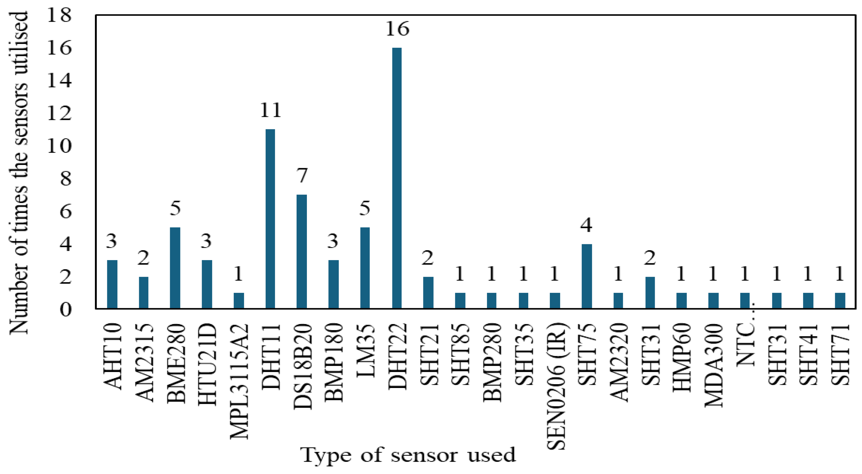
• Thermistors (the DHT22 and DHT11) and semiconductor-based sensors were the most utilized sensors in the studies found.
• Variations in calibration techniques and performance metrics were noted in the studies. A number of studies presented different performance metrics, limiting comparability between studies.

Environmental factors, notably solar radiation, were found to significantly affect sensor accuracy. Several studies that conducted sensor calibrations in outdoor environments reported sensor drifts attributed to solar radiation. Humidity also influences specific sensor types, particularly the DHT22, due to its dual capability to measure temperature and humidity. Other combined humidity and temperature sensing devices are suspected to encounter similar limitations; however, this remains unproven due to a lack of comprehensive studies in this area. While studies have recommended using radiation shields, their high cost limits their applicability in low-cost environmental monitoring initiatives. Alternatively, some research has proposed using machine learning algorithms to compensate for the impact of environmental factors on sensor accuracy [39].

Critical recommendations regarding the calibration and validation of low-cost air temperature sensors are provided within this review. For the standard validation or calibration method, it would be recommended to consider the following:

• Employ performance metrics, such as R² and RMSE, for standard validation, where R² measures model predictive accuracy and RMSE reflects the average deviation between actual and predicted readings.
• To account for bias, it is recommended that the mean error or average error be used, which accounts for the difference between the reference sensor and the calibrated sensor readings.
• Outline systematically the calibration procedure; this should include details on the calibration settings, including duration and conditions.
• Incorporating multiple temperature steps across varied ranges is necessary for accurate sensor performance evaluation in conjunction with the calibration model. This information will clearly outline how the sensor performs alongside the calibration performance model.
• Conducting a post-calibration assessment of sensor performance, especially in the same calibrating setting, since sensor performance can be affected when the setting is changed. This indicates that at least two calibration plans are required for accuracy, where the first calibration plan is carried out in the laboratory under the ideal conditions where sensor performance is optimum, after which a post-calibration assessment is carried out to assess improvement. The second calibration plan should be conducted in the setting where the sensor is to be deployed. Carrying out calibration under various conditions is important to improve reliability.
• Machine learning algorithms are recommended for outdoor settings; however, the choice of the models should be clearly investigated to ensure compatibility with the microcontroller and platform. The integration of machine learning not only refines calibration practices through automatic recalibration but also accounts for environmental factors as independent variables, thereby improving calibration curves.

6. Limitations

While this systematic review provides detailed findings and a synthesis of both calibration and sensor performance, several limitations must be acknowledged:

• Inconsistencies in the study reporting standards: Several studies lacked comprehensive descriptions of their calibration methodologies and, in certain instances, omitted critical performance metrics. Moreover, inconsistencies were identified in the reported evaluation parameters, which introduce uncertainties when attempting to synthesise results across different studies. These discrepancies hinder the feasibility of conducting robust meta-analyses, as the available data are often insufficient for reliable cross-study comparisons and require cautious interpretation.
• Variation in calibration and validation conditions: The absence of standardised temperature ranges, calibration durations, settings, and instrumentation has resulted in calibrations being performed under highly heterogeneous environmental conditions and with varying equipment. This methodological variability has contributed to significant discrepancies in the reported outcomes, thereby limiting the reliability of meta-analyses concerning both calibration models and sensor performance due to the lack of uniform calibration protocols.
• Variation in regional climatic conditions: Climatic and temperature variations across different geographic regions pose significant challenges to the interpretation of outdoor sensor and model calibrations. Environmental factors—such as solar radiation—may influence sensor performance differently depending on location-specific conditions. In cases where key parameters such as ambient temperature and outdoor conditions were not adequately reported, the interpretation of sensor and calibration model performance is further compromised, limiting the comparability and generalisability of findings.
• Sensor origin and assembly variability: Given the global distribution of the reviewed studies, variations in sensor suppliers, manufacturers, and assembly practices introduced additional uncertainties in the cross-comparison of sensor performance. In some cases, sensors were obtained from different sources or platforms that may not have been authorised distributors, potentially leading to inconsistencies in hardware quality or configuration. Such variability undermines the consistency and reliability of comparative analyses, highlighting the need for transparent reporting on sensor provenance and specifications.
• Lack of formal tools or software for bias assessment: As this review employed a manual evaluation of the risk of bias, certain uncertainties remain regarding the methodological quality of the included studies.

Despite the limitations of this review, a significant research gap was identified in the field of low-cost, commercially available air temperature sensors, suggesting that further investigation and research are necessary in this area, as these types of sensors could be a potential turning point in environmental monitoring and precision agriculture. Their applicability has not been fully exploited; to achieve this, the quality of their data needs to be validated and improved. Additionally, it was noted that despite these considerations, researchers often overlook the importance of calibration and validation, as many rely on factory calibrations without acknowledging that these factories do not specify how the sensors were manufactured, limiting their transparency. Aligning with the findings of [26,29], we present a call for the standardisation of low-cost sensor calibration. The implementation of a standard calibration technique will enable the reliability and accessibility of these sensors in both the environmental monitoring sector and the agricultural sector. Sensor calibration is the key to reliable and precise sensing instruments.

References

1. Gross Domestic Product and Agriculture Value Added 2013–2022. Global and Regional Trends. Available online: https://www.fao.org/statistics/highlights-archive/highlights-detail/gross-domestic-product-and-agriculture-value-added-2013-2022.-global-and-regional-trends/en (accessed on 16 November 2024).
2. World Bank. Purchasing Power Parities and the Size of World Economies: Results from the 2017 International Comparison Program; World Bank: Washington, DC, USA, 2020; ISBN 978-1-4648-1530-0. [Google Scholar]
3. Hashim, Z.K.; De Silva, A.G.S.D.; Hassouni, A.A.; Vona, V.M.; Bede, L.; Stencinger, D.; Horváth, B.; Zsebő, S.; Kulmány, I.M. Effects of Various Herbicide Types and Doses, Tillage Systems, and Nitrogen Rates on CO2 Emissions from Agricultural Land: A Literature Review. Agriculture 2024, 14, 1800. [Google Scholar] [CrossRef]
4. Kulmany, I.; Giczi, Z.; Beslin, A.; Bede, L.; Kalocsai, R.; Vona, V. Impact of Environmental and Soil Factors in the Prediction of Soil Carbon Dioxide Emissions under Different Tillage Systems. Ecocycles 2022, 8, 27–39. [Google Scholar] [CrossRef]
5. Juhász, C.; Huzsvai, L.; Kovács, E.; Kovács, G.; Tuba, G.; Sinka, L.; Zsembeli, J. Carbon Dioxide Efflux of Bare Soil as a Function of Soil Temperature and Moisture Content under Weather Conditions of Warm, Temperate, Dry Climate Zone. Agronomy 2022, 12, 3050. [Google Scholar] [CrossRef]
6. Precision Agriculture Definitions. Available online: https://www.grap.udl.cat/en/presentacio/que-fem/definicions-agricultura-de-precisio/index.html (accessed on 17 November 2024).
7. Srbinovska, M.; Gavrovski, C.; Dimcev, V.; Krkoleva, A.; Borozan, V. Environmental Parameters Monitoring in Precision Agriculture Using Wireless Sensor Networks. J. Clean. Prod. 2015, 88, 297–307. [Google Scholar] [CrossRef]
8. Vieira, M.A.M.; Coelho, C.N.; da Silva, D.C.; da Mata, J.M. Survey on Wireless Sensor Network Devices. In Proceedings of the IEEE Conference on Emerging Technologies and Factory Automation, Lisbon, Portugal, 16–19 September 2003; Volume 1, pp. 537–544, (Cat. No.03TH8696). [Google Scholar] [CrossRef]
9. Gandhi, N.; Petkar, O.; Armstrong, L.J. Rice Crop Yield Prediction Using Artificial Neural Networks. In Proceedings of the 2016 IEEE Technological Innovations in ICT for Agriculture and Rural Development (TIAR), Chennai, India, 15–16 July 2016; pp. 105–110. [Google Scholar] [CrossRef]
10. van Klompenburg, T.; Kassahun, A.; Catal, C. Crop Yield Prediction Using Machine Learning: A Systematic Literature Review. Comput. Electron. Agric. 2020, 177, 105709. [Google Scholar] [CrossRef]
11. Zsebő, S.; Bede, L.; Kukorelli, G.; Kulmány, I.M.; Milics, G.; Stencinger, D.; Teschner, G.; Varga, Z.; Vona, V.; Kovács, A.J. Yield Prediction Using NDVI Values from GreenSeeker and MicaSense Cameras at Different Stages of Winter Wheat Phenology. Drones 2024, 8, 88. [Google Scholar] [CrossRef]
12. Wheeler, T.R.; Craufurd, P.Q.; Ellis, R.H.; Porter, J.R.; Vara Prasad, P.V. Temperature Variability and the Yield of Annual Crops. Agric. Ecosyst. Environ. 2000, 82, 159–167. [Google Scholar] [CrossRef]
13. Asseng, S.; Foster, I.; Turner, N.C. The Impact of Temperature Variability on Wheat Yields. Glob. Change Biol. 2011, 17, 997–1012. [Google Scholar] [CrossRef]
14. Barash, H.; Silanikove, N.; Shamay, A.; Ezra, E. Interrelationships Among Ambient Temperature, Day Length, and Milk Yield in Dairy Cows Under a Mediterranean Climate. J. Dairy Sci. 2001, 84, 2314–2320. [Google Scholar] [CrossRef]
15. Carabaño, M.J.; Bachagha, K.; Ramón, M.; Díaz, C. Modeling Heat Stress Effect on Holstein Cows under Hot and Dry Conditions: Selection Tools. J. Dairy Sci. 2014, 97, 7889–7904. [Google Scholar] [CrossRef]
16. Sotvoldiev, X.; Tukxtasinov, D.; Zokirov, S.; Toxirova, S.; Abdullayeva, M.; Muhammadjonov, A. Review and Analysis of Methods of Automation of Temperature Measurement Process. E3S Web Conf. 2024, 592, 03024. [Google Scholar] [CrossRef]
17. Hu, K.A.; Runt, J.; Safari, A.; Newnham, R.E. Composite Thermistors. In Tailoring Multiphase and Composite Ceramics; Tressler, R.E., Messing, G.L., Pantano, C.G., Newnham, R.E., Eds.; Springer: Boston, MA, USA, 1986; pp. 475–479. ISBN 978-1-4612-9309-5. [Google Scholar]
18. Temperature Sensors: Types, How It Works, & Applications. Available online: https://www.encardio.com/blog (accessed on 20 January 2025).
19. Prasad, D.; Nath, V. An Overview of Temperature Sensors. In Proceedings of the Second International Conference on Microelectronics, Computing & Communication Systems (MCCS 2017); Nath, V., Mandal, J.K., Eds.; Springer: Singapore, 2019; pp. 777–784. [Google Scholar]
20. Blonquist, J.M., Jr.; Bugbee, B. Air Temperature. In Agroclimatology; John Wiley & Sons, Ltd.: Hoboken, NJ, USA, 2020; pp. 51–72. ISBN 978-0-89118-358-7. [Google Scholar]
21. Kloog, I.; Chudnovsky, A.; Koutrakis, P.; Schwartz, J. Temporal and Spatial Assessments of Minimum Air Temperature Using Satellite Surface Temperature Measurements in Massachusetts, USA. Sci. Total Environ. 2012, 432, 85–92. [Google Scholar] [CrossRef]
22. Garcia, J.L.M.I. Environmental & Economic Impact on Sustainable Development; WIT Press: Southampton, UK, 2016; ISBN 978-1-78466-245-5. [Google Scholar]
23. Feizizadeh, B.; Blaschke, T. Thermal Remote Sensing for Land Surface Temperature Monitoring: Maraqeh County, Iran. In Proceedings of the 2012 IEEE International Geoscience and Remote Sensing Symposium, Munich, Germany, 22–27 July 2012; pp. 2217–2220. [Google Scholar] [CrossRef]
24. Lewis, A.C.; Richard, P.W.; Schneidemesser, V.E. Low-Cost Sensors for the Measurement of Atmospheric Composition: Overview of Topic and Future Applications; WMO-No. 1215; World Health Organization (WMO): Geneva, Switzerland, 2018; ISBN 978-92-63-11215-6. [Google Scholar]
25. Tiele, A.; Esfahani, S.; Covington, J. Design and Development of a Low-Cost, Portable Monitoring Device for Indoor Environment Quality. J. Sens. 2018, 2018, 5353816. [Google Scholar] [CrossRef]
26. Chojer, H.; Branco, P.T.B.S.; Martins, F.G.; Alvim-Ferraz, M.C.M.; Sousa, S.I.V. Development of Low-Cost Indoor Air Quality Monitoring Devices: Recent Advancements. Sci. Total Environ. 2020, 727, 138385. [Google Scholar] [CrossRef]
27. Ferrero, A.; Scotti, V. Calibration. In Forensic Metrology. Research For Development; Springer International Publishing: Cham, Switzerland, 2022; pp. 95–106. [Google Scholar] [CrossRef]
28. González Rivero, R.A.; Morera Hernández, L.E.; Schalm, O.; Hernández Rodríguez, E.; Alejo Sánchez, D.; Morales Pérez, M.C.; Nuñez Caraballo, V.; Jacobs, W.; Martinez Laguardia, A. A Low-Cost Calibration Method for Temperature, Relative Humidity, and Carbon Dioxide Sensors Used in Air Quality Monitoring Systems. Atmosphere 2023, 14, 191. [Google Scholar] [CrossRef]
29. Karagulian, F.; Barbiere, M.; Kotsev, A.; Spinelle, L.; Gerboles, M.; Lagler, F.; Redon, N.; Crunaire, S.; Borowiak, A. Review of the Performance of Low-Cost Sensors for Air Quality Monitoring. Atmosphere 2019, 10, 506. [Google Scholar] [CrossRef]
30. Page, M.J.; McKenzie, J.E.; Bossuyt, P.M.; Boutron, I.; Hoffmann, T.C.; Mulrow, C.D.; Shamseer, L.; Tetzlaff, J.M.; Akl, E.A.; Brennan, S.E.; et al. The PRISMA 2020 Statement: An Updated Guideline for Reporting Systematic Reviews. BMJ 2021, 372, n71. [Google Scholar] [CrossRef]
31. Moola, S.; Munn, Z.; Sears, K.; Sfetcu, R.; Currie, M.; Lisy, K.; Tufanaru, C.; Qureshi, R.; Mattis, P.; Mu, P. Conducting Systematic Reviews of Association (Etiology): The Joanna Briggs Institute’s Approach. JBI Evid. Implement. 2015, 13, 163. [Google Scholar] [CrossRef] [PubMed]
32. Puspasari, F.; Satya, T.P.; Oktiawati, U.Y.; Fahrurrozi, I.; Prisyanti, H. Analisis Akurasi Sistem Sensor DHT22 berbasis Arduino terhadap Thermohygrometer Standar. J. Fis. Dan Apl. 2020, 16, 40–45. [Google Scholar] [CrossRef]
33. Hadi, S.; Labib, R.P.M.D.; Widayaka, P.D. Perbandingan Akurasi Pengukuran Sensor LM35 Dan Sensor DHT11 Untuk Monitoring Suhu Berbasis Internet Of Things. STRING Satuan Tulisan Ris. Dan Inov. Teknol. 2022, 6, 269–278. [Google Scholar] [CrossRef]
34. Baehaqi, M.; Rosyid, A.; Siswanto, A.; Subiyanta, E. Performance Testing of DHT11 and DS18B20 Sensors as Server Room Temperature Sensors. Mestro 2023, 5, 6–11. [Google Scholar] [CrossRef]
35. Utama, Y.A.K. Quality Comparison Between Temperature Sensors Using Arduino Pro Mini. E-Narodroid 2016, 2, 145–150. [Google Scholar] [CrossRef]
36. Satya, T.P.; Puspasari, F. Kajian Ketidakpastian Pengukuran Suhu Dan Kelembaban Udara Pada Sensor DHT22 Berbasis Arduino Uno. J. ILMU Fis. Univ. ANDALAS 2019, 11, 102–110. [Google Scholar] [CrossRef]
37. Koestoer, R.A.; Saleh, Y.A.; Roihan, I.; Harinaldi. A Simple Method for Calibration of Temperature Sensor DS18B20 Waterproof in Oil Bath Based on Arduino Data Acquisition System. AIP Conf. Proc. 2019, 2062, 020006. [Google Scholar] [CrossRef]
38. Bernardes, G.F.L.R.; Ishibashi, R.; Ivo, A.A.S.; Rosset, V.; Kimura, B.Y.L. Prototyping Low-Cost Automatic Weather Stations for Natural Disaster Monitoring. Digit. Commun. Netw. 2023, 9, 941–956. [Google Scholar] [CrossRef]
39. Yamamoto, K.; Togami, T.; Yamaguchi, N.; Ninomiya, S. Machine Learning-Based Calibration of Low-Cost Air Temperature Sensors Using Environmental Data. Sensors 2017, 17, 1290. [Google Scholar] [CrossRef]
40. Karami, M.; McMorrow, G.V.; Wang, L. Continuous Monitoring of Indoor Environmental Quality Using an Arduino-Based Data Acquisition System. J. Build. Eng. 2018, 19, 412–419. [Google Scholar] [CrossRef]
41. Pereira, P.F.; Ramos, N.M.M. Low-Cost Arduino-Based Temperature, Relative Humidity and CO2 Sensors–An Assessment of Their Suitability for Indoor Built Environments. J. Build. Eng. 2022, 60, 105151. [Google Scholar] [CrossRef]
42. Martinez, A.; Hernandez-Rodríguez, E.; Hernandez, L.; Schalm, O.; González-Rivero, R.A.; Alejo-Sánchez, D. Design of a Low-Cost System for the Measurement of Variables Associated With Air Quality. IEEE Embed. Syst. Lett. 2023, 15, 105–108. [Google Scholar] [CrossRef]
43. Mehmet, T. A Low-Cost Air Quality Monitoring System Based on Internet of Things for Smart Homes. J. Ambient. Intell. Smart Environ. 2022, 14, 351–374. [Google Scholar] [CrossRef]
44. Araújo, T.; Silva, L.; Moreira, A. Evaluation of Low-Cost Sensors for Weather and Carbon Dioxide Monitoring in Internet of Things Context. IoT 2020, 1, 286–308. [Google Scholar] [CrossRef]
45. Mobaraki, B.; Komarizadehasl, S.; Castilla Pascual, F.J.; Lozano-Galant, J.A. Application of Low-Cost Sensors for Accurate Ambient Temperature Monitoring. Buildings 2022, 12, 1411. [Google Scholar] [CrossRef]
46. Ali, A.S.; Zanzinger, Z.; Debose, D.; Stephens, B. Open Source Building Science Sensors (OSBSS): A Low-Cost Arduino-Based Platform for Long-Term Indoor Environmental Data Collection. Build. Environ. 2016, 100, 114–126. [Google Scholar] [CrossRef]
47. Jordão, M.D.L.; de Paiva, K.; Firmo, H.T.; Inácio, C.T.; Rotunno, O.C.; Lima, T.d.A.e. Low-Cost Automatic Station for Compost Temperature Monitoring. Rev. Bras. Eng. Agríc. Ambient. 2017, 21, 809–813. [Google Scholar] [CrossRef]
48. Yulizar, D.; Soekirno, S.; Ananda, N.; Prabowo, M.A.; Perdana, I.F.P.; Aofany, D. Performance Analysis Comparison of DHT11, DHT22 and DS18B20 as Temperature Measurement. In Proceedings of the 2nd International Conference on Science Education and Sciences 2022 (ICSES 2022), Lombok, Indonesia, 3–4 November 2022; Atlantis Press: Dordrecht, The Netherlands, 2023; pp. 37–45. [Google Scholar] [CrossRef]
49. Škultéty, E.; Pivarčiová, E.; Karrach, L. The Comparing of The Selected Temperature Sensors Compatible with The Arduino Platform. Manag. Syst. Prod. Eng. 2018, 26, 168–171. [Google Scholar] [CrossRef]
50. Kim, J.Y.; Abdel-Haleem, H.; Luo, Z.; Szczepanek, A. Open-Source Electronics for Plant Phenotyping and Irrigation in Controlled Environment. Smart Agric. Technol. 2023, 3, 100093. [Google Scholar] [CrossRef]
51. Satriya Wibawa, I.M.; Putra, I.K. Design of Air Temperature and Humidity Measurement Based on Arduino ATmega 328P with DHT22 Sensor. Int. J. Phys. Sci. Eng. 2022, 6, 9–17. [Google Scholar] [CrossRef]
52. Frei, M.; Deb, C.; Stadler, R.; Nagy, Z.; Schlueter, A. Wireless Sensor Network for Estimating Building Performance. Autom. Constr. 2020, 111, 103043. [Google Scholar] [CrossRef]
53. Gharghan, S.K. Energy-Efficient Remote Temperature Monitoring System for Patients Based on GSM Modem and Microcontroller. J. Commun. 2017, 12, 433–442. [Google Scholar] [CrossRef]
54. Martín-Garín, A.; Millán-García, J.A.; Baïri, A.; Millán-Medel, J.; Sala-Lizarraga, J.M. Environmental Monitoring System Based on an Open Source Platform and the Internet of Things for a Building Energy Retrofit. Autom. Constr. 2018, 87, 201–214. [Google Scholar] [CrossRef]
55. Liu, H.; Wang, B.; Sun, X.; Li, T.; Liu, Q.; Guo, Y. DCSCS: A Novel Approach to Improve Data Accuracy for Low Cost Meteorological Sensor Networks. Inf. Technol. J. 2014, 13, 1640–1647. [Google Scholar] [CrossRef]
56. Routis, G.; Roussaki, I. Low Power IoT Electronics in Precision Irrigation. Smart Agric. Technol. 2023, 5, 100310. [Google Scholar] [CrossRef]
57. Jouini, O.; Sethom, K.; Namoun, A.; Aljohani, N.; Alanazi, M.H.; Alanazi, M.N. A Survey of Machine Learning in Edge Computing: Techniques, Frameworks, Applications, Issues, and Research Directions. Technologies 2024, 12, 81. [Google Scholar] [CrossRef]
58. Wang, B.; Gu, X.; Ma, L.; Yan, S. Temperature Error Correction Based on BP Neural Network in Meteorological Wireless Sensor Network. Int. J. Sens. Netw. 2017, 23, 265. [Google Scholar] [CrossRef]
59. Sihombing, Y.A.; Listiari, S. Detection of Air Temperature, Humidity and Soil pH by Using DHT22 and pH Sensor Based Arduino Nano Microcontroller. In AIP Conference Proceedings, Proceedings of the 1st International Conference on Physics and Applied Physics (The 1st ICP&AP), Medan, Indonesia, 12–13 September 2019; AIP Publishing: Melville, NY, USA, 2020; Volume 2221, pp. 100008-1–100008-6. [Google Scholar] [CrossRef]
60. Firdaus, R.; Murti, M.A.; Alinursafa, I. Air Quality Monitoring System Based Internet of Things (IoT) Using LPWAN LoRa. In Proceedings of the 2019 IEEE International Conference on Internet of Things and Intelligence System (IoTaIS), Bali, Indonesia, 5–7 November 2019; pp. 195–200. [Google Scholar] [CrossRef]
61. Mobaraki, B.; Komarizadehasl, S.; Pascual, F.J.C.; Antonio, J.; Galant, L. Determination of Environmental Parameters Based on Arduino Based Low-Cost Sensors. In Proceedings of the RTCEE International Conference, Online, 10–11 September 2020; ISBN 978-0-6489449-0-4. [Google Scholar]
62. Ahmad, Y.A.; Surya Gunawan, T.; Mansor, H.; Hamida, B.A.; Fikri Hishamudin, A.; Arifin, F. On the Evaluation of DHT22 Temperature Sensor for IoT Application. In Proceedings of the 2021 8th International Conference on Computer and Communication Engineering (ICCCE), Kuala Lumpur, Malaysia, 22–23 June 2021; pp. 131–134. [Google Scholar] [CrossRef]
63. Sunardi, A.; Agus, D.; Aditya, H.; Susila, W. Online Air Velocity Control, Temperature and Humidity Monitoring System for Clean Room Using Raspberry Pi. IOP Conf. Ser. Mater. Sci. Eng. 2019, 550, 012011. [Google Scholar] [CrossRef]
64. Megantoro, P.; Iswanto; Pramudita, B.A. IoT-Based Weather Station with Python User Interface for Measurement Technique of Educational Purpose. AIP Conf. Proc. 2020, 2296, 020027. [Google Scholar] [CrossRef]
65. Shahadat, B.S.A.; Ayon, I.S.; Khatun, R.M. Efficient IoT Based Weather Station. In Proceedings of the 2020 IEEE International Women in Engineering (WIE) Conference on Electrical and Computer Engineering (WIECON-ECE), Bhubaneswar, India, 26–27 December 2020; pp. 227–230. [Google Scholar] [CrossRef]
66. Mesas-Carrascosa, F.J.; Verdú Santano, D.; Meroño, J.E.; Sánchez de la Orden, M.; García-Ferrer, A. Open Source Hardware to Monitor Environmental Parameters in Precision Agriculture. Biosyst. Eng. 2015, 137, 73–83. [Google Scholar] [CrossRef]
67. Carre, A.; Williamson, T. Design and Validation of a Low Cost Indoor Environment Quality Data Logger. Energy Build. 2018, 158, 1751–1761. [Google Scholar] [CrossRef]
68. Du Plessis, R.; Kumar, A.; Hancke, G.; Silva, B. A Wireless System for Indoor Air Quality Monitoring. In Proceedings of the IECON 2016–42nd Annual Conference of the IEEE Industrial Electronics Society, Florence, Italy, 24–27 October 2016; pp. 5409–5414. [Google Scholar] [CrossRef]
69. Aashiq, M.N.M.; Kurera, W.T.C.C.; Thilekaratne, M.G.S.P.; Saja, A.M.A.; Rouzin, M.R.M.; Neranjan, N.; Yassin, H. An IoT-Based Handheld Environmental and Air Quality Monitoring Station. Acta IMEKO 2023, 12, 1–9. [Google Scholar] [CrossRef]
70. Hartono, J.R.; Utama, D.N. Temperature, Humidity, and Light Intensity Monitoring System Using Internet of Things on Mesh Network. Int. J. Comput. Digit. Syst. 2024, 16, 1–10. [Google Scholar]
71. Chodorek, A.; Chodorek, R.R.; Yastrebov, A. Weather Sensing in an Urban Environment with the Use of a UAV and WebRTC-Based Platform: A Pilot Study. Sensors 2021, 21, 7113. [Google Scholar] [CrossRef] [PubMed]
72. Fissore, I.V.; Arcamone, G.; Astolfi, A.; Barbaro, A.; Carullo, A.; Gallione, D.; Giusto, E.; Chiavassa, P.; Clerico, M.; Fantucci, S.; et al. Multi-Sensor Device for Traceable Monitoring of Indoor Environmental Quality. Sensors 2024, 24, 2893. [Google Scholar] [CrossRef] [PubMed]
73. Joice, A.; Tufaique, T.; Tazeen, H.; Igathinathane, C.; Zhang, Z.; Whippo, C.; Hendrickson, J.; Archer, D. Applications of Raspberry Pi for Precision Agriculture—A Systematic Review. Agriculture 2025, 15, 227. [Google Scholar] [CrossRef]
74. Concas, F.; Mineraud, J.; Lagerspetz, E.; Varjonen, S.; Liu, X.; Puolamäki, K.; Nurmi, P.; Tarkoma, S. Low-Cost Outdoor Air Quality Monitoring and Sensor Calibration: A Survey and Critical Analysis. ACM Trans. Sens. Netw. 2021, 17, 1–44. [Google Scholar] [CrossRef]
75. Sun, X.; Yan, S.; Wang, B.; Xia, L.; Liu, Q.; Zhang, H. Air Temperature Error Correction Based on Solar Radiation in an Economical Meteorological Wireless Sensor Network. Sensors 2015, 15, 18114–18139. [Google Scholar] [CrossRef]
76. Young, D.T.; Chapman, L.; Muller, C.L.; Cai, X.-M.; Grimmond, C.S.B. A Low-Cost Wireless Temperature Sensor: Evaluation for Use in Environmental Monitoring Applications. Am. Meteorol. Soc. J. Atmos. Ocean. Technol. 2014, 31, 938–944. [Google Scholar] [CrossRef]
77. Faroqi, A.; Efendi, M.R.; Ismail, D.T.; Darmalaksana, W. Design of Arduino Uno Based Duck Egg Hatching Machine With Sensor DHT22 and PIR Sensor. In Proceedings of the 2020 6th International Conference on Wireless and Telematics (ICWT), Yogyakarta, Indonesia, 3–4 September 2020; pp. 1–4. [Google Scholar] [CrossRef]
78. Kumar Sai, K.B.; Mukherjee, S.; Parveen Sultana, H. Low Cost IoT Based Air Quality Monitoring Setup Using Arduino and MQ Series Sensors With Dataset Analysis. Procedia Comput. Sci. 2019, 165, 322–327. [Google Scholar] [CrossRef]
79. Wang, B.; Cai, H.; Jia, Q.; Fu, L.; Pan, H.; Li, B. Smart Temperature Sensor Design and High-Density Water Temperature Monitoring in Estuarine and Coastal Areas. Sensors 2023, 23, 7659. [Google Scholar] [CrossRef]
Figure 1. Classification of keywords according to the PEO framework.
Atmosphere 16 00842 g001
Figure 2. Adapted PRISMA flow diagram representing summary of study collection.
Atmosphere 16 00842 g002
Figure 3. Map of the world showing which countries the studies collected were from.
Atmosphere 16 00842 g003
Figure 4. The bar graph shows how many times each sensor is mentioned across the collected studies.
Atmosphere 16 00842 g004
Figure 5. Bar graph showing how studies utilized different models.
Atmosphere 16 00842 g005