Global Methane Retrieval, Monitoring, and Quantification in Hotspot Regions Based on AHSI/ZY-1 Satellite

Abstract

Methane is the second largest greenhouse gas. The detection of methane super-emitters and the quantification of their emission rates are necessary for the implementation of methane emission reduction policies to mitigate global warming. High-spectral-resolution satellites such as Gaofen-5 (GF-5), EMIT, GHGSat, and MethaneSAT have been successfully employed to detect and quantify methane point source leaks. In this study, a matched filter (MF) algorithm is improved using data from the EMIT instrument and applied to data from the Advanced Hyperspectral Imager (AHSI) onboard the Ziyuan-1 (ZY-1) satellite. Validation by comparison with EMIT′s L2 XCH₄ products shows the good performance of the improved MF algorithm, in spite of the lower spectral resolution of AHSI/ZY-1 in comparison with other point source imagers. The improved MF algorithm applied to AHSI/ZY-1 data was used to detect and quantify methane super-emitters in global methane hotspot regions. The results show that the improved MF algorithm effectively suppresses noise in retrieval results over both land and ocean surfaces, enhancing algorithm robustness. Sixteen methane plumes were detected in global hotspot regions, originating from coal mines, oil and gas fields, and landfills, with emission rates ranging from 0.57 to 78.85 t/h. The largest plume was located at an offshore oil and gas field in the Gulf of Mexico, with instantaneous emissions nearly equal to the combined total of the other 15 plumes. The findings demonstrate that AHSI, despite its lower spectral resolution, can detect sources with emission rates as small as 571 kg/h and achieve faster retrieval speeds, showing significant potential for global methane monitoring. Additionally, this study highlights the need to focus on methane emissions from marine sources, alongside terrestrial sources, to efficiently implement reduction strategies.

1. Introduction

Climate change is a critical environmental challenge. The latest assessment report from the United Nations Intergovernmental Panel on Climate Change (IPCC) in 2023 highlights that, as a result of human activities, the global average temperature has increased by 1.1 °C compared to pre-industrial levels. If current trends continue, it is likely that the temperature will exceed 1.5 °C above pre-industrial levels at some point between 2030 and 2050 [1]. However, as reported by Copernicus, the first year when this happened was already in 2024 (https://climate.copernicus.eu/copernicus-2024-first-year-exceed-15degc-above-pre-industrial-level, last visited on 28 February 2025). The continued rise in greenhouse gas (GHG) emissions is the dominant factor triggering warming, and common GHGs mainly include water vapor (H₂O), carbon dioxide (CO₂), and methane (CH₄) [2]. Methane is one of the most significant anthropogenic greenhouse gases in the Earth′s climate system. Since the pre-industrial era, atmospheric methane concentrations have more than doubled, exceeding 1940 parts per billion (ppb) [3]. The rising levels of methane, combined with its strong capability to absorb thermal infrared radiation emitted by the Earth, have made it the second most important greenhouse gas, following carbon dioxide [4]. Since the atmospheric lifetime of CH₄ (≈9 years) is an order of magnitude shorter than that of CO₂ (≈100–500 years), reduction in methane emissions can lead to a more rapid decrease or stabilization of its atmospheric concentration over decadal timescales. This makes methane a highly effective target for emission reduction and mitigation strategies aimed at achieving short- and medium-term climate goals. By addressing methane emissions, significant progress can be made in curbing near-term global warming potential [5].

Industrial activities linked to fossil fuel production contribute approximately 30% of global anthropogenic methane emissions, with the oil and gas (O&G) industry being one of the largest sources (https://gml.noaa.gov/ccgg/carbontracker-ch4/index.html, last visited on 2 March 2025). Methane emissions from this sector are particularly challenging to quantify due to their variable nature, often resulting from leaks, equipment malfunctions, or design deficiencies. The quantity, duration, and frequency of these emissions can fluctuate significantly across regions, equipment types, and transmission networks, making consistent monitoring and measurement difficult. As such, accurate estimation and mitigation of methane emissions in the O&G industry remain complex but critical for effective climate action [6]. In addition to these unpredictable factors, this component of emissions can also come from excess natural gas from human-controlled combustion and venting processes. Additionally, significant methane leakage and emissions from coal mines and landfills have been confirmed by numerous studies [7] and are similarly difficult to monitor directly with ground-based equipment [8]. Since all of these activities have the potential to result in super-emissions and may account for a large percentage of regional emissions, it is necessary to accurately observe and quantify these sources.

Imaging spectrometers are capable of measuring solar and infrared reflected radiation at a wide range of wavelengths, ranging from the visible and near-infrared (VNIR: 400–1000 nm) to the short-wave infrared (SWIR: 1000–2500 nm) and thermal infrared. The spectra measured by these instruments contain information on the occurrence and concentrations of trace gases and greenhouse gases in the atmosphere [9]. Methane has two absorption bands in the SWIR: a weak absorption band in the 1650 nm window and a strong absorption band in the 2300 nm window. These absorption bands can be used to detect the concentration of methane in the atmosphere, from which methane emissions can be derived [10].

In recent years, multispectral and hyperspectral satellite remote sensing technology has become a key tool for monitoring methane emissions by virtue of its inherent higher sensitivity, wider observational range, and high revisit capability [11]. The FTS (Fourier Transform Spectrometer) onboard the GOSAT and GOSAT-2 satellites provides high-resolution spectral measurements of atmospheric radiation at wavelengths from the near-infrared to the thermal infrared that can be used to retrieve column-integrated concentrations of methane [12,13]. Since 2017, the TROPOMI sensor onboard the Sentinel-5p satellite has been used to produce daily global methane concentration data at 7 × 5.5 km² resolution. TROPOMI is an area flux mapper that can monitor methane emissions at global to regional scales [14,15]. For the quantification of methane emissions from point sources, sensors are required that provide both high spatial and spectral resolution. Such point source imagers include GHGSat [16], PRISMA [17], EnMAP [18], EMIT [19], MethaneSAT [20], Tanager-1 [21,22], and the Chinese GF-5 [23] and ZY-1 [24] series of satellites. In addition, the verification methods of methane concentrations obtained by these imagers mainly include verification based on simulated synthetic images and real emission sources on the surface. The verification based on simulated synthetic images mainly uses the “LES method [17,25,26]”, and the other way mainly includes “single-blind test [27,28]”, “comparison of ground-based or airborne measurements of actual leakage sources [29,30]”, and “comparison of emission inventories [31,32,33]”. In these two test methods, the methane column concentrations obtained by satellite imagers are well consistent with the reference results, providing confidence for related research work. An overview of methane area flux mappers and point source imagers is provided in

Table 1. Overview of methane area flux mappers and point satellite/sensor.

Satellite /Sensor	Launch (Year)	Country	Methane Window Range (nm)	Spectral Resolution (nm)	Spatial Resolution	Reference
GOSAT/FTS	2009	Japan	1560–1720	0.05	10.5 km	[12]
GOSAT-2/FTS-2	2018	Japan	1560–1690	0.05	9.7 km	[13]
GHGSat/WAF-P	2016, 2020–2023	Canada	1600–1700	0.3	25 m	[16]
Sentiel-5P/TROPOMI	2017	Netherlands	2305–2385	0.25	7 km × 5.5 km	[14,15]
GF-5/AHSI	2018	China	1600–1700, 2200–2500	5–10	30 m	[22]
ZY-1/AHSI	2019	China	1600–1700, 2200–2500	10–20	30 m	[23]
PRISMA/HYC	2019	Italy	1600–1700, 2200–2510	10	30 m	[17]
EnMAP/HSI	2022	Germany	1600–1700, 2200–2510	6.5–10	30 m	[18]
ISS/EMIT	2022	United States	1600–1700, 2200–2493	7.5	60 m	[19]
MethaneSAT	2024	United States	1598–1683	0.25	100 m × 400 m	[20]
Tanager-1	2024	United States	1600–1700, 2200–2500	5	30 m	[21,22]

. In Table 1, spatial resolution refers to the size of the sub-satellite pixel, i.e., at nadir.

For the retrieval of methane concentrations from the observed spectra, they can be matched to spectra simulated using a full physics method involving detailed radiative transfer calculations. Alternatively, the observed spectrum can be fitted to a background spectrum convolved with a target methane absorption spectrum at the appropriate wavelengths [13].

In this paper, the latter method, referred to as the matched filter (MF) method, is improved using L1B irradiance data and L2B methane column concentrations (XCH₄) from the EMIT instrument (on the International Space Station) developed by NASA′s Jet Propulsion Laboratory (JPL) [34]. The improved MF algorithm is applied to data from the Advanced Hyperspectral Imager (AHSI) aboard the Ziyuan-1 (ZY-1) and GaoFen-5 (GF-5) satellites for monitoring of methane emission sources. The emission rates from typical methane sources (including coal mines, oil and gas fields, and landfills) are quantified based on the Integrated Mass Enhancement (IME) model.

2. Materials and Methods

2.1. Data Used

2.1.1. EMIT and AHSI/ZY-1 Data

In this study, EMIT′s L1B irradiance and L2B XCH₄ data were used to evaluate the performance of the algorithms and assess their accuracy. Additionally, irradiance data from the AHSI sensors onboard the ZY-1E and ZY-1F satellites, along with the radiatively corrected L1 irradiance product, were utilized as inputs for methane column concentration inversion, aimed at monitoring and quantifying methane plumes in global emission hotspot regions.

The Earth Surface Mineral Dust Source Investigation (EMIT) imaging spectrometer, developed by NASA, was initially designed for studying mineral distribution in arid and semi-arid regions. However, later, the sensor was also used to detect global super-emission sources of carbon dioxide and methane. EMIT was launched on 14 July 2022 and mounted on the International Space Station (ISS), where it captures detailed spectral data at a spatial resolution of 60 m, with a swath width of 75 km and a spectral range of 400–2500 nm (with a spectral resolution of 7.5 nm) across 285 spectral channels. This advanced capability enables precise monitoring of greenhouse gas emissions from space [35].

The ZY-1E/F satellites were successfully launched on 12 September 2019 and 26 December 2021, respectively. Both satellites operate in sun-synchronous orbits within an isochronous grouping. The AHSI sensors on these satellites provide images with a spatial resolution of 30 m and a swath width of 60 km. However, the number of spectral bands is limited to 166, and the spectral resolution is coarser, ranging from 10 to 20 nm (10 nm in the VNIR band and 20 nm in the SWIR band) [36].

The satellite image data and point locations used in this study are listed in

Table 2. Details of the data used in this study.

Sensor/Satellite	Date	Image ID
EMIT/ISS	21 April 2024	EMIT_L1B_RAD_001_20240421T184222_2411212_043
EMIT/ISS	5 February 2023	EMIT_L1B_RAD_001_20230205T171255_2303612_007
AHSI/ZY1F	16 April 2024	ZY1F_AHSI_W92.32_N19.70_20240416_012087_L1A0000712903
AHSI/ZY1F	6 July 2023	ZY1F_AHSI_E87.60_N44.12_20230707_008006_L1A0000479173
AHSI/ZY1E	26 October 2020	ZY1E_AHSI_E54.02_N38.83_20201026_005889_L1A0000192157
AHSI/ZY1E	19 February 2021	ZY1E_AHSI_E54.39_N38.38_20210219_007553_L1A0000244210
AHSI/ZY1E	6 December 2023	ZY1E_AHSI_E112.40_N35.73_20231206_022179_L1A0000687604
AHSI/ZY1E	27 November 2023	ZY1E_AHSI_E6.09_N31.66_20231127_022057_L1A0000683681
AHSI/ZY1F	29 April 2024	ZY1F_AHSI_W102.02_N31.73_20240429_012274_L1A0000724023
AHSI/ZY1F	19 May 2024	ZY1F_AHSI_W104.17_N32.17_20240519_012561_L1A0000739948
AHSI/ZY1E	17 January 2024	ZY1E_AHSI_W103.75_N32.17_20240117_022795_L1A0000708354
AHSI/ZY1F	31 August 2023	ZY1F_AHSI_W80.86_N33.95_20240414_012058_L1A0000710869

, including 2 views of EMIT images and 10 views of ZY-1E/F images.

2.1.2. GEOS-FP Reanalysis of Wind Speed Data

In this study, wind speed data are needed as auxiliary data to estimate emissions from point source plumes. To this end, we use the hourly U₁₀ wind speed reanalysis products from the Goddard Earth Observing System Forward Processing (GEOS-FP), at a resolution of 0.3125 degrees in longitude and 0.25 degrees in latitude. The data are updated daily and published as a global file every hour. We use the global wind speed data closest to the overpass time of the satellite used to detect the methane plume and extract the wind speed at the location of the plume [37].

2.2. Incremental Methane Column Concentration Inversion Based on Matched Filter

Matched filter (MF) is a data-driven statistical method based on extracting the magnitude of perturbations in hyperspectral images due to absorption by a target gas, in this case, methane, to indirectly measure the increment of the methane concentration with respect to the background. The MF method has been widely used to characterize the amount of trace gases in the atmosphere. The idea behind the matched filter retrieval chosen in this paper is that each input spectrum can be represented as a spectrum with no methane enhancement in the background, plus a background-based perturbation of the input spectrum due to variations in the concentration of the methane column [38,39].

This algorithm assumes that the background radiation is a sufficiently homogeneous multivariate Gaussian distribution with mean (μ) and covariance (Σ), and that the methane enhancement possesses sparsity, i.e., the methane enhancement does not affect the background distribution characteristics [40,41]:

$$x_b~N\left(\mu ,\Sigma \right)$$

(1)

The radiative transfer can be modeled as ΔXCH₄ in the atmosphere according to the Beer–Lambert law:

$$x=x_b\cdot {\mathrm{e}}^{-\Delta XC{H}_4\left(i\right)\cdot k}$$

(2)

where x is the spectrum of radiation received by the sensor, x_b is the reference background radiation, XCH₄ is the dry-air column-averaged mixing ratio of methane, and ΔXCH₄(i) is the pixel-by-pixel enhancement of the methane column mixing ratio with respect to the background in ppb, which is also the target variable for the inversion in this study. k is the unit absorption spectrum of CH₄, which characterizes the sensitivity of the observed radiation to the ΔXCH₄ perturbation. Linearization of Equation (2) using a first-order Taylor series expansion yields

$$x=x_b-\Delta XC{H}_4\cdot x_b\cdot k+n$$

(3)

where n is the residual difference between the observed irradiance and the background irradiance.

The following equation is used:

$$t=x_b\cdot k$$

(4)

The above equation can be written as

$$x=x_b-\Delta XC{H}_4\cdot t+n$$

(5)

where t represents the target spectrum, defined as the absorption equivalent radiance spectrum per unit methane concentration relative to the background. $\Delta XC{H}_4\cdot t$ reflects the enhancement of the background irradiance caused by the methane plume. Figure 1 shows an example of the target spectrum of the AHSI/ZY-1 sensor calculated using the spectral response function of the AHSI sensor.

Since the background is assumed to follow a normal distribution, n similarly follows a normal distribution, i.e.,

$$n=x-\left(x_b-\Delta XC{H}_4\cdot t\right)~N\left(\mu ,\Sigma \right)$$

(6)

The distribution of enhanced pixels in the plume is characterized by sparsity, so that $x_b$ and Σ can be estimated from the mean (μ) and covariance of the observed radiance difference. By minimizing the Gaussian log-likelihood, the optimal estimate is given as

$$\Delta XC{H}_4\left(x\right)={\displaystyle \frac{{\left(x-\mu \right)}^T{\Sigma }^{-1}t}{t^T{\Sigma }^{-1}t}}$$

(7)

The above equation is the basic form of the calculation using matched filters [42]. Since the absolute radiance from surfaces with a low albedo is smaller as the surface albedo decreases, detecting the target signal over a surface with low albedo will be more difficult. In this study, the Albedo-Corrected L1-reweighted ISTA matched filter algorithm for surface (Albedo Corr. RWL1 MF), proposed by Foote et al. (2020) [25], is used, which is based on the idea that anomalously high values due to methane emissions from multiple point sources may affect a few thousand pixels in satellite data. However, the affected pixels constitute only a small fraction of the whole scene. Sparse processing of the data can effectively eliminate the influence of background features and thus efficiently detect target-induced anomalies in areas with complex surface types. At the same time, the algorithm can utilize pixel-by-pixel specific albedo factors to adjust the target spectrum. Here, the background irradiance average and the input image x are used as the parameters for the calculation of f [25]:

$$f={\displaystyle \frac{x^T\mu }{{\mu }^T\mu }}$$

(8)

where f is a pixel-specific scalar. Then, it is scaled by f and thus normalized with the albedo term.

The advantage of the MF algorithm lies in its simplicity, as compared with full-physics methods, which require consideration of the complex transmission process of solar radiation through the atmosphere during the inversion process. Instead, the MF method directly extracts the target covariates from the spectral perturbation information inherent in the hyperspectral image data. The MF method significantly enhances inversion efficiency while maintaining a reasonable degree of accuracy. As a result, it has been widely adopted and implemented in numerous satellite-based remote sensing applications [43].

2.3. Identifying Methane Plumes in ΔXCH₄ Images

Typically, apparent concentrations are higher than the real concentrations due to albedo anomalies caused by various surface features (e.g., solar panels, reflective rooftops, lakes, meadows, etc.) and weather conditions (clouds, snow) [26]. The complexity of the surface can lead to highly variable wind directions, making it challenging to accurately extract the plume morphology through fully automated methods. Therefore, this study employs a semi-automatic approach to identify methane plumes from enhanced methane column concentration images. The process involves the following steps: First, single-point noise in the image is removed using low-pass filtering. Next, the connectivity of the plume is assessed, and a connectivity threshold is set to extract regions with connected areas, which are then identified as potential plume scenes. Finally, by integrating high-resolution surface images with wind speed data, suspected plume scenes are confirmed as real plumes if a genuine emission source exists below them and if methane concentrations in the plume decrease in all directions. High-resolution surface images are sourced from Tianmap (https://image.tianditu.gov.cn/multidate, accessed on 28 February 2025), while wind speed data are derived from the 1 h averaged U₁₀ dataset of NASA’s GEOS-FP meteorological reanalysis product, which offers a high spatial resolution (0.3125° × 0.25°) and is easily accessible [44].

Additionally, testing in this study revealed that while the plume direction should generally align with the wind direction, with concentration decreasing in that direction, discrepancies can arise between the suspected plume direction and the wind direction in the reanalyzed data. This misalignment is primarily due to the temporal and spatial resolution limitations of the reanalyzed data and inherent errors. However, if the morphology of the suspected plume remains intact and a confirmed emission source is identified in the high-resolution surface image, the suspected plume is treated as a real plume in this study. Wind speed also plays a critical role in plume formation. If the wind speed is too low, plume formation becomes difficult, and plume characteristics may not be observable in the enhanced methane column concentration image. Conversely, if the wind speed is too high, the plume may become diluted, leading to a lower methane concentration that may fall below the detection threshold of the satellite. Therefore, locating methane leaks or emissions, especially when the emission source is unknown, requires a combination of multiple observational data sources.

2.4. Accounting for Emission Flux Rates

For estimation of the emission flux, the Integrated Mass Enhancement (IME) model [45] was used in this study to calculate the methane mass in the plume relative to the background from the retrieved plume images. The emission rate is then calculated using Equation (9) by inputting the wind speed and plume length as follows:

$$IME=k{\displaystyle \sum }_{i=1}^n\Delta XC{H}_4\left(i\right)$$

(9)

In the above equation, n is the number of pixels in the plume region, and k is the mass coefficient of methane in the air column observed by the sensor. The observed air column is calculated from the volumetric mixing ratio to the mass according to Avogadro′s law, taking into account the spatial resolution of the sensor, using the concept of scale height, i.e., an atmospheric column of with a height of 8 km (https://astro.unl.edu/mobile/scaleheight/sh_bg1.html, accessed on 21 April 2025) in which all methane is compressed to a constant density a STP. Different sensors have different mass coefficients k due to their different spatial resolutions. After calculation, k_AHSI = 5.155 × 10⁻³ kg/ppb for AHSI/ZY-1 with a spatial resolution of 30 m, and k_EMIT = 2.062 × 10⁻² kg/ppb for EMIT with a spatial resolution of 60 m. The IME is the Integrated Mass Enhancement of the plume (in kg). After obtaining the IME, the emission rate was obtained by calculating the effective wind speed U_eff (unit: m/s):

$$U_{eff}=\alpha \cdot U_{10}+\beta$$

(10)

where U₁₀ is the GEOS-FP re-analysis 10 m wind speed (unit: m/s), and they possess the conversion relationship of Equation (10), where α and β are determined by large eddy simulation. Because α and β do not vary significantly globally [23], in this paper, the values adopted for α and β were the estimates for the Permian Basin (α = 0.34 and β = 0.44) [32].

$$Q={\displaystyle \frac{U_{eff}\cdot IME}{L}}$$

(11)

In the above equation, Q is the methane emission rate (in kg/h), and L is the plume length (in m), defined as the square root of the plume mask area.

2.5. Error Analysis

In order to estimate the uncertainty in Q, the random errors in the IME and U₁₀ are propagated to the 1-σ precision error in Q [46]. The U10 term is the main error contribution, and assuming a 50% random error in wind speed for the GEOS-FP U10 data, the random distribution of U₁₀ values corresponding to this 50% random error is converted to a distribution of Q values using Equation (12) [47]. This U10 error contribution is quadratically combined with the standard error of the IME to obtain the final Q random error. In addition, since the determination of the plume mask is somewhat subjective and not well quantified, this study similarly does not consider the effect of mask identification on the emission rate, and there is no specific threshold to distinguish between plume pixels and background pixels [33]. We considered pixels with ∆XCH₄ values more than twice the noise level (2σ) as statistically significant (in order to retain statistically significant pixels with p < 0.05). In summary, the 1σ accuracy error of Q is propagated by random errors in ∆XCH₄ and wind speed, where wind speed is the main source of error. The equation is given below:

$$\sigma ={\displaystyle \frac{\sqrt{{\left(U_{eff}\cdot {\sigma }_{IME}\right)}^2+{\left(IME\cdot {\sigma }_{U_{eff}}\right)}^2}}{L}}$$

(12)

$${\sigma }_{U_{eff}}=\alpha \cdot U_{10}\cdot 50\%$$

(13)

3. Results

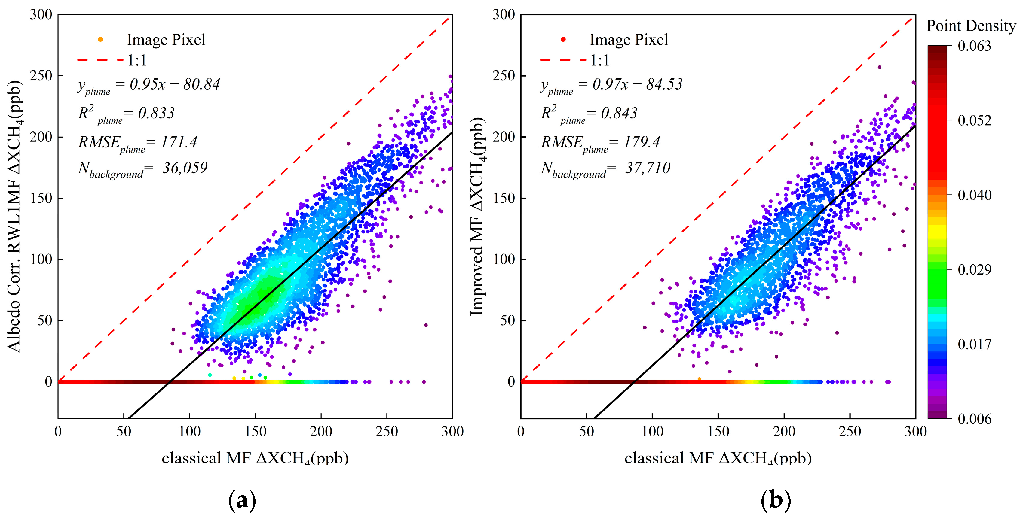
3.1. Performance Analysis of Algorithm Inversion for Sea–Land Surface

In this study, two locations were selected for validation of the algorithm: the Gulf of Mexico and the Permian Basin. The ocean surface of the Gulf of Mexico, as a scene with a uniform and clean background, can be approximated as having no extreme changes in reflectivity due to changes in elevation, vegetation, and construction facilities, which reduces the complexity of the background. In contrast, the Permian Basin, located in the United States, is a classic hotspot for methane emissions, with some disturbing factors on the surface due to the oil and gas pipelines running through the area, as well as certain undulations in the terrain and relatively complex surface facilities. The comparison of information from the two different types of background allows for the assessment of the algorithm′s inversion performance in different environments.

In this study, an EMIT image (Image ID: 20240421T184222) of an oil and gas field located in the upper Gulf of Mexico is used to validate the algorithm over a homogeneous background scenario. Figure 2 shows an RGB satellite image and a high-resolution image of the site. The RGB satellite image is a color composite from AHSI/ZY-1, while the high-resolution image has been obtained from [Reuters] (https://www.reuters.com/markets/commodities/pemex-platform-mexico-leaked-clouds-methane-even-after-un-alert-data-shows-2024-02-09/, accessed on 28 February 2025). Figure 3 shows two scenes with the methane plume: EMIT′s L2B XCH₄ product (Figure 3a) and the XCH₄ plume retrieved from the EMIT L1B radiance product using the improved MF algorithm developed in this study (Figure 3b). Due to the clean background, both images show a morphologically intact plume, with the background noise effectively suppressed. However, the EMIT L2B product still contains some random noise and noise bands due to sensor limitations. In contrast, in the plume retrieved using the improved MF algorithm, the noise is significantly reduced. While some discrete high-value points remain, the absence of corresponding sources indicates that there are no additional small offshore oil and gas wells leaking. Moreover, there are some differences in the patterns of the plumes shown in Figure 3. Notably, the divergence of the plume retrieved using the improved MF algorithm is smaller, and the variation in the concentration gradient is larger. As a result, the methane plume patterns can be more clearly distinguished and are easier to extract. Numerically, the maximum column concentration increment of the methane plume in the EMIT L2B product is 536.25 ppb, corresponding to an instantaneous emission rate of 16.97 t/h. The inversion using the improved MF algorithm yields a column concentration increment of 815.2 ppb, which is 1.52 times higher than the EMIT result, and an emission rate of 17.04 t/h, differing by only 0.41% from the emission rate provided by EMIT. The results from the MF algorithm are more reliable, with the discrepancy in column concentration increment likely due to the algorithm’s noise reduction and plume area adjustment, maintaining the emission rate constant.

Previous studies have shown that the maximum values of column concentration increments obtained from different algorithmic inversions can vary significantly, even for the same image [39]. These maximum values may be influenced by anomalies arising from other factors, such as algorithm characteristics and surface type. Consequently, in this study, rather than using the maximum value of the plume column concentration as the sole metric for evaluating algorithm accuracy, both the emission rate and the overall concentration distribution of the plume are considered as performance indicators. Ideally, after MF calculation, the column concentration increment of the area without a plume should be 0. Therefore, the number of pixels in this part can measure the cleanliness of the background. As illustrated in the histograms of Figure 4, which show the distribution of the column concentrations of the plumes presented in Figure 3, it is evident that the EMIT plume follows a Gaussian distribution from 0 to 300 ppb, with a higher number of pixels at lower concentrations. This suggests a high level of background noise and an unclear boundary between the plume and the background. In contrast, the histogram of the plume distribution obtained using the improved MF algorithm shows a very high and narrow peak at 0 ppb, indicating the background, followed by initially very small frequencies of occurrence for very low ΔXCH₄, which then increase as ΔXCH₄ increases to the peak near 75 ppb, whereafter they gradually decreasing to 625 ppb. This indicates a clearer separation between the background and the plume, with noise significantly reduced.

To assess the enhancement of the improved MF algorithm proposed in this study compared to previous methods for terrestrial backgrounds, and to further validate the reliability of the inversion results, we used another EMIT image (Image ID: 20230205T171255), over a terrestrial background in the Permian Basin, as the input. The inversion performance of the MF algorithm proposed by Foote (2020) [25] (Albedo Corr. RWL1 MF) and improved MF applied to EMIT L1B data was compared with the classical MF algorithm (RMF), and the results are presented in Figure 5, Figure 6 and Figure 7. Given that the selected images contain only a single emission source, the expected result is that all areas outside the plume should either show background values or random noise, with these values ideally close to zero. The ΔXCH₄ images in Figure 5 and the corresponding histograms in Figure 6 show that the RMF algorithm produces a more complete basic plume morphology. However, the distribution of values within the plume is suboptimal, with most column concentrations ranging from 200 ppb to 300 ppb. As a result, it is difficult to distinguish the plume boundary from the noisy background. In contrast, the Albedo Corr. RWL1 MF algorithm significantly reduces background noise, preserving the plume′s morphology. The column concentration within the plume decreases gradually from the emission source in a consistent direction, and the distribution of concentration values from the plume center to its boundary aligns with expected physical patterns. The plume image derived using the improved MF method further minimizes noise by more effectively segmenting the plume from the background. It is evident from a comparison of the histograms in Figure 6 that the number of noise pixels within the plume section has been further reduced by using the improved MF algorithm, leading to a more refined and accurate representation of the methane plume.

Figure 7 presents scatter density plots of ΔXCH₄ retrieved using the improved MF algorithm or Foote (2020) [25]’s Albedo Corr. RWL1 MF versus ΔXCH₄ data retrieved using the classical MF method. Due to the large number of pixels eliminated from the background, a direct comparison of all scatter points is statistically not significant. Therefore, we extracted and compared only the scatter points within the plume region. The straight lines in the figures represent the least square fits to the data, with the statistical metrics R² and RMSE provided in the figures. N_background denotes the number of points with a vertical coordinate of 0, representing the background of the ΔXCH₄ image after removing the plume. From the scatter plots, it is evident that each plot can be roughly divided into two parts: the first part consists of scatter points near the vertical axis (0), and the second part contains scatter points distributed around the fitted straight line. The scatter points near the fitted line indicate the comparison of the plume regions in the ΔXCH₄ image after inversion by both algorithms. In the comparison between Albedo Corr. RWL1 MF and RMF, the fitted straight line is y = 0.95x − 80.84, with R² = 0.833 and RMSE = 171.4 (N = 36,059). Albedo Corr. RWL1 MF effectively removes a large portion of the noise from the RMF while maintaining consistency in the plume distribution. In the comparison between the MF and RMF used in this study, it is clear that much of the noise is further reduced, and there is better consistency in the distribution of the plumes in comparison with Albedo Corr. RWL1 MF. The fitted line has a slope of 0.97 and R² = 0.843, indicating a better fit compared to Albedo Corr. RWL1 MF. However, the RMSE of 179.4 suggests that the scatter points are somewhat more dispersed.

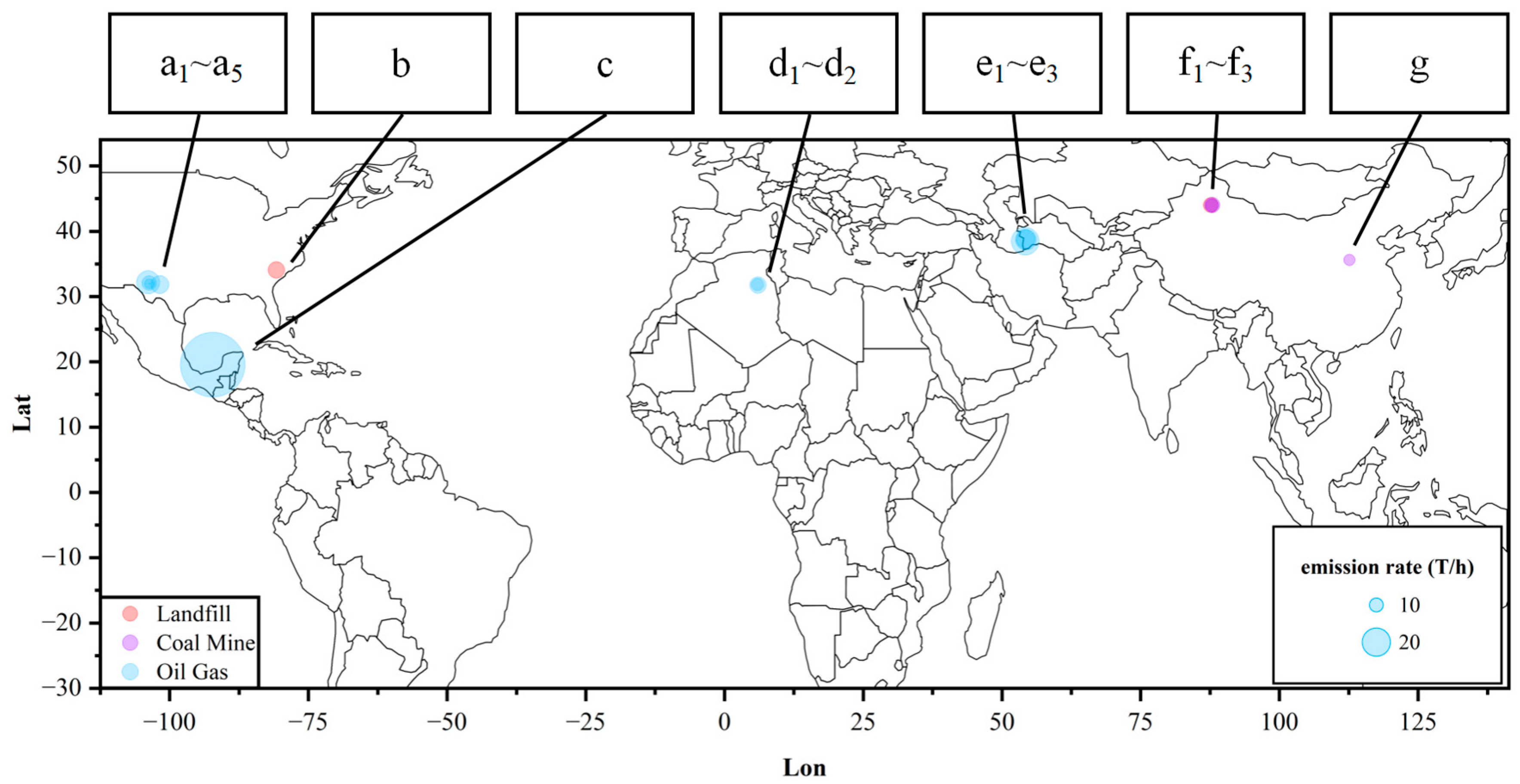
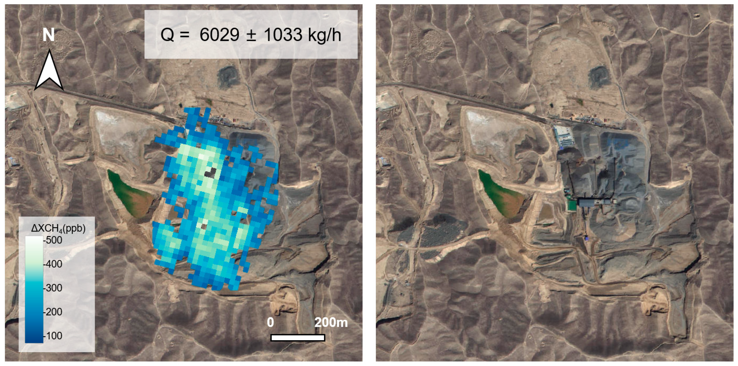
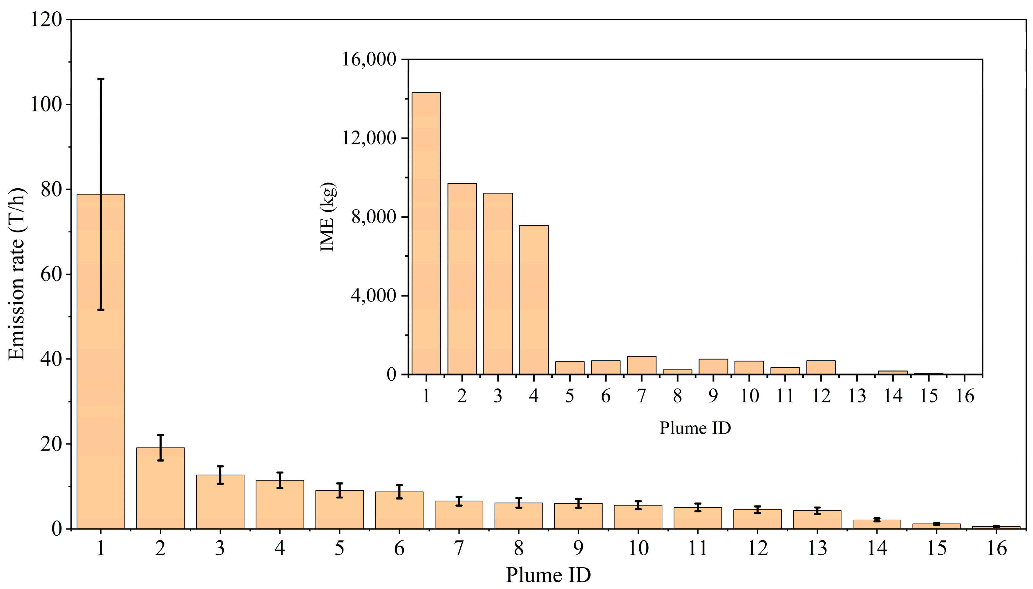
3.2. Detection and Quantification of Global Methane Hotspot Plume Emissions Based on ZY-1 Satellite

In Section 3.1, the inversion performance and accuracy of the MF algorithm used in this study for sea and land backgrounds were analyzed, with comparisons to algorithms from previous studies. In this section, the AHSI sensor onboard the ZY-1E/F satellites is used to detect and quantify a portion of the methane plume in global methane hotspot regions.

The map in Figure 8 shows methane emission hotspots, which are used in this study. A total of 16 methane plumes are identified, distributed across the Permian Basin (USA), South Carolina (USA), the Gulf of Mexico, Algeria, the Turkmenistan Basin, and regions in Xinjiang and Shanxi in China (

Table 3. Plume locations, dates, emission rates, and source types for the 16 plumes identified in this study through inversion. The code in the first column refers to the locations as explained in the text.

Plume ID	Emission Source Type	Emission Rate (kg/h)	Date	Latitude	Longitude
a1	Oil and Gas	4535 ± 791	29 April 2024	31°51′31.7″ N	101°45′52.2″ W
a2	Oil and Gas	9086 ± 1659	19 May 2024	32°12′03.9″ N	103°54′53.6″ W
a3	Oil and Gas	571 ± 95	17 January 2024	31°57′09.7″ N	103°40′14.4″ W
a4	Oil and Gas	2154 ± 358	17 January 2024	31°57′15.6″ N	103°40′41.2″ W
a5	Oil and Gas	1170 ± 195	17 January 2024	32°04′13.1″ N	103°43′39.5″ W
b	Landfill	6543 ± 1018	14 April 2024	34°06′26.2″ N	80°46′17.8″ W
c	Oil and Gas	78,847 ± 2719	16 April 2024	19°34′1.61″ N	92°14′15.25″ W
d1	Oil and Gas	8754 ± 1586	27 November 2023	31°46′42.79″ N	5°59′42.51″ E
d2	Oil and Gas	5072 ± 919	27 November 2023	31°50′7.60″ N	5°56′36.74″ E
e1	Oil and Gas	11,453 ± 1845	26 October 2020	38°51′09.7″ N	54°14′12.8″ E
e2	Oil and Gas	12,698 ± 2046	26 October 2020	38°41′21.9″ N	54°18′53.7″ E
e3	Oil and Gas	19,142 ± 2977	19 February 2021	38°29′37.7″ N	54°11′47.0″ E
f1	Landfill	5588 ± 958	6 July 2023	44°2′20.84″ N	87°51′59.79″ E
f2	Coal Mines	6029 ± 1033	6 July 2023	44°0′39.99″ N	87°50′11.32″ E
f3	Coal Mines	4298 ± 762	31 August 2023	44°0′39.99″ N	87°50′11.32″ E
g	Coal Mines	6146 ± 1126	6 December 2023	35°37′7.65″ N	112°36′34.14″ E

). These plumes correspond to emissions from 12 oil and gas facilities, two landfills, and two coal mines. Different colored circles in the map represent various types of emission sources, with the size of each circle indicating the magnitude of the emission rate at that location. Due to geographic proximity, some circles may overlap, and the opacity of the legends has been adjusted to prevent visual obstruction. Each plume is numbered, with plumes sharing the same letter indicating emission sources located within the same region. The emission rates, dates, coordinates, and types of leakage sources for the 16 plumes identified in this study through inversion are summarized in Table 3. The source with the lowest emission rate is located in an oil and gas field in the Permian Basin in the USA with a rate of Q = 571 ± 95 kg/h, and the source with the highest rate is located in the Zaap-C field in the Gulf of Mexico with a rate of Q = 78,847 ± 2719 kg/h.

Among the emission sources in Table 3, a₁–a₅ represent five sources located in the Permian Basin in the USA, all attributed to oil and gas field discharge or leakage. Source b corresponds to a landfill in South Carolina, USA, while source c is linked to methane leakage from an offshore oil and gas field in the Gulf of Mexico. Sources d₁–d₂ represent emissions from an oil and gas field in Algeria, and e₁–e₃ are associated with methane leakage from oil and gas fields in Turkmenistan. Sources f₁–f₃ and g are related to a landfill (f₁) and three coal mines in China. The methane plume results and surface facilities at f₂ are presented in Figure 9. Furthermore, the 16 plumes are ranked according to their emission rates, with the IME plotted schematically in Figure 10.

4. Discussion

In this study, a matched filter (MF) algorithm has been improved, and the results were evaluated using data from the EMIT instrument on the ISS. The improved MF algorithm was applied to data from the Advanced Hyperspectral Imager (AHSI) onboard the Ziyuan-1 (ZY-1) satellite. The improvement of the MF algorithm for XCH₄ retrieval was investigated by comparison with EMITS XCH₄ data from two sources. One source was located over the ocean, i.e., the Zaap-C oil and gas field in the Gulf of Mexico, and the other site was a terrestrial location over the Permian Basin in the USA. The results show the better performance of the improved MF algorithm over that of the EMIT data, and both datasets (improved MF and EMITS L2B) were much better than those from the RMF algorithm. The improved MF algorithm was applied to data from the AHSI sensor on the ZY-1 satellite to detect global methane hotspots and evaluate the retrieval performance of AHSI/ZY-1 in different regions based on the 16 retrieved methane plumes. Point source emission rates were determined for all 16 sources. The results demonstrate that despite its spectral resolution being limited to 10–20 nm, the AHSI sensor on ZY-1E/F offers relatively strong methane detection capabilities on a global scale. Additionally, the spectral resolution of ZY-1 is only half that of the GF-5 sensor, and it has fewer spectral bands (ZY-1 has 180 bands compared to GF-5’s 330), resulting in higher inversion efficiency and timeliness when using the same algorithm. This is particularly significant for the timely detection and mitigation of large-scale methane leaks in the future. Furthermore, while most previous studies have focused on land-based methane emission sources, offshore emissions have often been overlooked due to their distance from populated areas. However, the results of this study highlight the detection of emissions from the Zaap-C oil and gas field located in the Gulf of Mexico. The methane emission rates from Zaap-C were quantified at 78,847 ± 2719 kg/h, and assuming homogeneous leakage, this would amount to approximately 6.9 × 10⁴ t of methane leaking annually. This finding underscores the importance of detecting offshore methane leaks as part of efforts to reduce methane emissions globally.

At the same time, this study also calculated the IME of each plume. This analysis shows that the emission rate does not exhibit a direct correlation with the IME. In fact, when calculating emission rates, factors such as wind speed, plume area, and plume distribution pattern must also be considered, requiring a more comprehensive approach in future, more accurate assessments.

5. Conclusions

The matched filter algorithm proposed by Foote (2020) [25], aimed at reducing random noise in the inverted images and improving the inversion speed, was optimized utilizing EMIT products and used with data from the AHSI/ZY-1 sensor to investigate global methane emission hotspot areas. The AHSI results were used to quantify methane point source emissions. The key findings of this study are as follows:

(1)

Optimizing the background covariance estimation method within the matched filter algorithm not only reduces the algorithm′s dependence on the quality of hyperspectral data but also effectively diminishes random noise in the background. This enhancement ensures that inversion speed is maintained while improving the robustness of the algorithm and the reliability of the inversion results.

(2)

This study demonstrates that, despite the lower spectral resolution of AHSI compared with other point source imagers, the optimized algorithm can detect emissions as low as 571 ± 95 kg/h. This detection threshold is comparable to the 500 kg/h threshold identified by previous research using the AHSI/GF-5, which has a higher spectral resolution. Moreover, the smaller number of spectral bands of AHSI/ZY-1 compared to AHSI/GF-5 results in significant advantages in inversion efficiency, suggesting its great potential for large-scale production of global methane plume products.

(3)

AHSI successfully detected and quantified methane emissions from the offshore Zaap-C oil and gas field in the Gulf of Mexico, a super-emission source. The detected emission rate of 78,847 ± 2719 kg/h is close to the combined emission rates of the other 15 plumes, highlighting the importance of addressing methane leaks not only from land-based facilities but also from offshore sources, which are often harder to detect due to their distance from populated areas.

Despite the demonstrated capability of AHSI in methane point source inversion and quantification, several challenges remain in methane inversion. These include uncertainties in the reanalyzed wind speed and inaccuracies in the plume shape, which introduce errors and uncertainties in emission rate calculations. Additionally, refining the methane absorption spectra used in the inversion algorithm is crucial for improving the accuracy of column concentration inversion. To enhance this accuracy, it is necessary to develop methane absorption spectra that match the specific load and observation parameters for different sensor configurations.

References

1. Albós, A.C. Predictions of Our Future Global Climate: Models, Scenarios, and Projections. In Climate Change for Astronomers: Causes, Consequences, and Communication; IOP Astronomy: Bristol, UK, 2024; pp. 3-1–3-18. [Google Scholar]
2. Sarfraz, M. Global Warming Cause and Impact on Climate Change. Int. J. Emerg. Knowl. Stud. 2024, 3, 198–204. Available online: https://ijeks.com/wp-content/uploads/2024/08/IJEKS-3-05-005.pdf (accessed on 16 February 2025).
3. Lan, X.; Thoning, K.W.; Dlugokencky, E.J. Trends in Globally-Averaged CH4, N2O, and SF6 Determined from NOAA Global Monitoring Laboratory Measurements; Version 2025-02; NOAA Global Monitoring Laboratory: Boulder, CO, USA, 2025. [Google Scholar] [CrossRef]
4. Xing, Y.; Wang, X. Impact of Agricultural Activities on Climate Change: A Review of Greenhouse Gas Emission Patterns in Field Crop Systems. Plants 2024, 13, 2285. [Google Scholar] [CrossRef]
5. Saunois, M.; Martinez, A.; Poulter, B.; Zhang, Z.; Raymond, P.; Regnier, P.; Canadell, J.G.; Jackson, R.B.; Patra, P.K.; Bousquet, P.; et al. Global Methane Budget 2000–2020. Earth Syst. Sci. Data Discuss. 2024, preprint. [Google Scholar] [CrossRef]
6. Vollrath, C. Methane Emissions from the Global Oil and Gas Industry: A Scoping Review to Characterize Research Trends, Knowledge Gaps, and Priorities. Master’s Thesis, University of Calgary, Calgary, AB, Canada, 2022. Available online: https://prism.ucalgary.ca/handle/1880/115218 (accessed on 16 February 2025).
7. Rani, A.; Pundir, A.; Verma, M.; Joshi, S.; Verma, G.; Andjelković, S.; Babić, S.; Milenković, J.; Mitra, D. Methanotrophy: A Biological Method to Mitigate Global Methane Emission. Microbiol. Res. 2024, 15, 634–654. [Google Scholar] [CrossRef]
8. Schuit, B.J.; Maasakkers, J.D.; Bijl, P.; Mahapatra, G.; Berg, A.-W.V.D.; Yaakoub, M.; Pandey, S.; Lorente, A.; Borsdorff, T.; Houweling, S.; et al. Automated detection and monitoring of methane super-emitters using satellite data. Atmos. Chem. Phys. Discuss. 2023, 23, 9071–9098. [Google Scholar] [CrossRef]
9. Matoušková, E. Hyperspectral Imaging and Its Terrestrial Applications. Ph.D. Thesis, Czech Technical University, Prague, Czech, 2021. [Google Scholar]
10. Wang, H.; Fan, X.; Jian, H.; Yan, F. Exploiting the Matched Filter to Improve the Detection of Methane Plumes with Sentinel-2 Data. Remote Sens. 2024, 16, 1023. [Google Scholar] [CrossRef]
11. Irakulis-Loitxate, I.; Guanter, L.; Maasakkers, J.D.; Zavala-Araiza, D.; Aben, I. Satellites detect abatable super-emissions in one of the world’s largest methane hotspot regions. Environ. Sci. Technol. 2022, 56, 2143–2152. [Google Scholar] [CrossRef] [PubMed]
12. Parker, R.; Boesch, H.; Cogan, A.; Fraser, A.; Feng, L.; Palmer, P.I.; Messerschmidt, J.; Deutscher, N.; Griffith, D.W.T.; Notholt, J.; et al. Methane observations from the Greenhouse Gases Observing SATellite: Comparison to ground-based TCCON data and model calculations. Geophys. Res. Lett. 2011, 38. [Google Scholar] [CrossRef]
13. Suto, H.; Kataoka, F.; Kikuchi, N.; Knuteson, R.O.; Butz, A.; Haun, M.; Buijs, H.; Shiomi, K.; Imai, H.; Kuze, A. Thermal and near-infrared sensor for carbon observation Fourier-transform spectrometer-2 (TANSO-FTS-2) on the Greenhouse Gases Observing Satellite-2 (GOSAT-2) during its first year on orbit. Atmos. Meas. Tech. Discuss. 2020, 14, 2013–2039. [Google Scholar] [CrossRef]
14. Lorente, A.; Borsdorff, T.; Butz, A.; Hasekamp, O.; de Brugh, J.A.; Schneider, A.; Wu, L.; Hase, F.; Kivi, R.; Wunch, D.; et al. Methane retrieved from TROPOMI: Improvement of the data product and validation of the first 2 years of measurements. Atmos. Meas. Tech. 2021, 14, 665–684. [Google Scholar] [CrossRef]
15. Jacob, D.J.; Varon, D.J.; Cusworth, D.H.; Dennison, P.E.; Frankenberg, C.; Gautam, R.; Guanter, L.; Kelley, J.; McKeever, J.; Ott, L.E.; et al. Quantifying methane emissions from the global scale down to point sources using satellite observations of atmospheric methane. Atmos. Chem. Phys. 2022, 22, 9617–9646. [Google Scholar] [CrossRef]
16. Varon, D.J.; McKeever, J.; Jervis, D.; Maasakkers, J.D.; Pandey, S.; Houweling, S.; Aben, I.; Scarpelli, T.; Jacob, D.J. Satellite discovery of anomalously large methane point sources from oil/gas production. Geophys. Res. Lett. 2019, 46, 13507–13516. [Google Scholar] [CrossRef]
17. Guanter, L.; Irakulis-Loitxate, I.; Gorroño, J.; Sánchez-García, E.; Cusworth, D.H.; Varon, D.J.; Cogliati, S.; Colombo, R. Mapping methane point emissions with the PRISMA spaceborne imaging spectrometer. Remote Sens. Environ. 2021, 265, 112671. [Google Scholar] [CrossRef]
18. Guanter, L.; Kaufmann, H.; Segl, K.; Foerster, S.; Rogass, C.; Chabrillat, S.; Kuester, T.; Hollstein, A.; Rossner, G.; Chlebek, C.; et al. The EnMAP Spaceborne Imaging Spectroscopy Mission for Earth Observation. Remote Sens. 2015, 7, 8830–8857. [Google Scholar] [CrossRef]
19. Thorpe, A.K.; Green, R.O.; Thompson, D.R.; Brodrick, P.G.; Chapman, J.W.; Elder, C.D.; Irakulis-Loitxate, I.; Cusworth, D.H.; Ayasse, A.K.; Duren, R.M.; et al. Attribution of individual methane and carbon dioxide emission sources using EMIT observations from space. Sci. Adv. 2023, 9, eadh2391. [Google Scholar] [CrossRef]
20. Hamburg, S.; Gautam, R.; Zavala-Araiza, D. MethaneSAT-A New Tool Purpose-Built to Measure Oil and Gas Methane Emissions from Space. In Proceedings of the Abu Dhabi International Petroleum Exhibition and Conference, Abu Dhabi, United Arab Emirates, 31 October–3 November 2022; p. D011S007R002. [Google Scholar] [CrossRef]
21. Planet Labs PBC. Planet Hyperspectral. 2024. Available online: https://www.planet.com/products/hyperspectral/ (accessed on 13 April 2025).
22. Hu, K.; Feng, X.; Zhang, Q.; Shao, P.; Liu, Z.; Xu, Y.; Wang, S.; Wang, Y.; Wang, H.; Di, L.; et al. Review of Satellite Remote Sensing of Carbon Dioxide Inversion and Assimilation. Remote Sens. 2024, 16, 3394. [Google Scholar] [CrossRef]
23. He, Z.; Gao, L.; Liang, M.; Zeng, Z.-C. A survey of methane point source emissions from coal mines in Shanxi province of China using AHSI on board Gaofen-5B. Atmos. Meas. Tech. 2024, 17, 2937–2956. [Google Scholar] [CrossRef]
24. Sherw Chen, L.; Sui, X.; Liu, R.; Chen, H.; Li, Y.; Zhang, X.; Chen, H. Mapping Alteration Minerals Using ZY-1 02D Hyperspectral Remote Sensing Data in Coalbed Methane Enrichment Areas. Remote Sens. 2023, 15, 3590. [Google Scholar] [CrossRef]
25. Foote, M.D.; Dennison, P.E.; Thorpe, A.K.; Thompson, D.R.; Jongaramrungruang, S.; Frankenberg, C.; Joshi, S.C. Fast and accurate retrieval of methane concentration from imaging spectrometer data using sparsity prior. IEEE Trans. Geosci. Remote Sens. 2020, 58, 6480–6492. [Google Scholar] [CrossRef]
26. Pei, Z.; Han, G.; Mao, H.; Chen, C.; Shi, T.; Yang, K.; Ma, X.; Gong, W. Improving quantification of methane point source emissions from imaging spectroscopy. Remote Sens. Environ. 2023, 295, 113652. [Google Scholar] [CrossRef]
27. Sherwin, E.D.; Rutherford, J.S.; Chen, Y.; Aminfard, S.; Kort, E.A.; Jackson, R.B.; Brandt, A.R. Single-blind validation of space-based point-source detection and quantification of onshore methane emissions. Sci. Rep. 2023, 13, 3836. [Google Scholar] [CrossRef] [PubMed]
28. Sherwin, E.D.; El Abbadi, S.H.; Burdeau, P.M.; Zhang, Z.; Chen, Z.; Rutherford, J.S.; Chen, Y.; Brandt, A.R. Single-blind test of nine methane-sensing satellite systems from three continents. Atmos. Meas. Tech. 2024, 17, 765–782. [Google Scholar] [CrossRef]
29. Dowd, E.; Manning, A.J.; Orth-Lashley, B.; Girard, M.; France, J.; Fisher, R.E.; Lowry, D.; Lanoisellé, M.; Pitt, J.R.; Stanley, K.M.; et al. First validation of high-resolution satellite-derived methane emissions from an active gas leak in the UK. Atmos. Meas. Tech. 2024, 17, 1599–1615. [Google Scholar] [CrossRef]
30. Karacan, C.Ö.; Irakulis-Loitxate, I.; Field, R.A.; Warwick, P.D. Temporal and spatial comparison of coal mine ventilation methane emissions and mitigation quantified using PRISMA satellite data and on-site measurements. Sci. Total Environ. 2025, 975, 179268. [Google Scholar] [CrossRef]
31. Li, F.; Sun, S.W.; Zhang, Y.G.; Feng, C.X.; Chen, C.H.; Mao, H.Q.; Liu, Y.N. Mapping methane super-emitters in China and United States with GF5-02 hyperspectral imaging spectrometer. Natl. Remote Sens. Bull. 2024, 28, 1986–2001. [Google Scholar] [CrossRef]
32. Irakulis-Loitxate, I.; Guanter, L.; Liu, Y.-N.; Varon, D.J.; Maasakkers, J.D.; Zhang, Y.; Chulakadabba, A.; Wofsy, S.C.; Thorpe, A.K.; Duren, R.M.; et al. Satellite-based survey of extreme methane emissions in the Permian basin. Sci. Adv. 2021, 7, eabf4507. [Google Scholar] [CrossRef] [PubMed]
33. Han, G.; Pei, Z.; Shi, T.; Mao, H.; Li, S.; Mao, F.; Ma, X.; Zhang, X.; Gong, W. Unveiling unprecedented methane hotspots in China’s leading coal production hub: A satellite mapping revelation. Geophys. Res. Lett. 2024, 51, e2024GL109065. [Google Scholar] [CrossRef]
34. Green, R.O.; Mahowald, N.; Ung, C.; Thompson, D.R.; Bator, L.; Bennet, M.; Bernas, M.; Blackway, N.; Bradley, C.; Cha, J.; et al. The Earth surface mineral dust source investigation: An Earth science imaging spectroscopy mission. In Proceedings of the 2020 IEEE Aerospace Conference, Big Sky, MT, USA, 7–14 March 2020; IEEE: Piscataway, NJ, USA, 2020; pp. 1–15. [Google Scholar] [CrossRef]
35. NASA Earth Science. Meet EMIT: NASA’s Newest Imaging Spectrometer. NASA Earth Data. 2022. Available online: https://www.earthdata.nasa.gov/news/feature-articles/meet-emit-newest-imaging-spectrometer (accessed on 21 April 2025).
36. SAS Clouds. ZY-102D Remote Sensing Satellite. Available online: https://www.sasclouds.com/chinese/satellite/chinese/zy102d (accessed on 21 April 2025).
37. Arnold, N.; Putman, W.; Freitas, S.; Takacs, L.; Rabenhorst, S. Impacts of New Atmospheric Physics in the Updated GEOS FP System (Version 5.25); NASA Global Modeling and Assimilation Office Reserch Brief: Greenbelt, MD, USA, 2020; Volume 9. [Google Scholar]
38. Thorpe, A.K.; Frankenberg, C.; Roberts, D.A. Retrieval techniques for airborne imaging of methane concentrations using high spatial and moderate spectral resolution: Application to AVIRIS. Atmos. Meas. Tech. 2014, 7, 491–506. [Google Scholar] [CrossRef]
39. Thorpe, A.; Frankenberg, C.; Aubrey, A.; Roberts, D.; Nottrott, A.; Rahn, T.; Sauer, J.; Dubey, M.; Costigan, K.; Arata, C.; et al. Mapping methane concentrations from a controlled release experiment using the next generation airborne visible/infrared imaging spectrometer (AVIRIS-NG). Remote Sens. Environ. 2016, 179, 104–115. [Google Scholar] [CrossRef]
40. Thompson, D.R.; Thorpe, A.K.; Frankenberg, C.; Green, R.O.; Duren, R.; Guanter, L.; Hollstein, A.; Middleton, E.; Ong, L.; Ungar, S. Space-based remote imaging spectroscopy of the Aliso Canyon CH4 superemitter. Geophys. Res. Lett. 2016, 43, 6571–6578. [Google Scholar] [CrossRef]
41. Foote, M.D.; Dennison, P.E.; Sullivan, P.R.; O’Neill, K.B.; Thorpe, A.K.; Thompson, D.R.; Cusworth, D.H.; Duren, R.; Joshi, S.C. Impact of scene-specific enhancement spectra on matched filter greenhouse gas retrievals from imaging spectroscopy. Remote Sens. Environ. 2021, 264, 112574. [Google Scholar] [CrossRef]
42. Thompson, D.R.; Leifer, I.; Bovensmann, H.; Eastwood, M.; Fladeland, M.; Frankenberg, C.; Gerilowski, K.; Green, R.O.; Kratwurst, S.; Krings, T.; et al. Real-time remote detection and measurement for airborne imaging spectroscopy: A case study with methane. Atmos. Meas. Tech. 2015, 8, 4383–4397. [Google Scholar] [CrossRef]
43. Ayasse, A.K.; Dennison, P.E.; Foote, M.; Thorpe, A.K.; Joshi, S.; Green, R.O.; Duren, R.M.; Thompson, D.R.; Roberts, D.A. Methane Mapping with Future Satellite Imaging Spectrometers. Remote Sens. 2019, 11, 3054. [Google Scholar] [CrossRef]
44. El Akkraoui, A.; Privé, N.C.; Errico, R.M.; Todling, R. The GMAO Hybrid 4D-EnVar Observing System Simulation Experiment Framework. Mon. Weather Rev. 2023, 151, 1717–1734. [Google Scholar] [CrossRef]
45. Zhang, S.; Ma, J.; Zhang, X.; Guo, C. Atmospheric remote sensing for anthropogenic methane emissions: Applications and research opportunities. Sci. Total Environ. 2023, 893, 164701. [Google Scholar] [CrossRef]
46. Cusworth, D.H.; Duren, R.M.; Yadav, V.; Thorpe, A.K.; Verhulst, K.; Sander, S.; Hopkins, F.; Rafiq, T.; Miller, C.E. Synthesis of methane observations across scales: Strategies for deploying a multitiered observing network. Geophys. Res. Lett. 2020, 47, e2020GL087869. [Google Scholar] [CrossRef]
47. Varon, D.J.; Jervis, D.; McKeever, J.; Spence, I.; Gains, D.; Jacob, D.J. High-frequency monitoring of anomalous methane point sources with multispectral Sentinel-2 satellite observations. Atmos. Meas. Tech. 2021, 14, 2771–2785. [Google Scholar] [CrossRef]
Figure 1. Example of a target spectrum of the AHSI/ZY-1 sensor.
Atmosphere 16 00510 g001
Figure 2. Images of the Zaap-C oil and gas field in the Gulf of Mexico: (a) RGB color composite from AHSI/ZY-1; (b) high-resolution image obtained from [Reuters].
Atmosphere 16 00510 g002
Figure 3. Methane plumes emitted from the Zaap-C oil and gas field: ΔXCH4 image from EMIT L2B (a) and the improved MF algorithm applied to EMIT L1B data (b).
Atmosphere 16 00510 g003
Figure 4. Comparison between the EMIT algorithm and the MF algorithm used in this study to invert the ΔXCH4 numerical distribution: EMIT L2B XCH4 (a) and the improved MF algorithm applied to EMIT L1B data XCH4 (b).
Atmosphere 16 00510 g004
Figure 5. ΔXCH4 retrieved using a classical MF method as reference (a), the Foote (2020) [25] MF algorithm (b), and the improved MF method (c), all applied to EMIT data over a terrestrial background in the Permian Basin.
Atmosphere 16 00510 g005
Figure 6. Histograms of ΔXCH4 derived from the scenes presented in Figure 5. (a) a classical MF method; (b) the Foote (2020) [25] MF algorithm ; (c) the improved MF method.
Atmosphere 16 00510 g006
Figure 7. Scatter density plots of ΔXCH4 retrieved using the improved MF algorithm (a) or the Foote (2020) [25] algorithm (b) versus ΔXCH4 reference data retrieved using the classical MF method.
Atmosphere 16 00510 g007
Figure 8. Survey of methane plumes in global methane hotspots.
Atmosphere 16 00510 g008
Figure 9. A methane plume and its ground facilities in Xinjiang Uygur Autonomous Region.
Atmosphere 16 00510 g009
Figure 10. Emission rate and IME of 16 methane plumes.
Atmosphere 16 00510 g010