Comparison of Sensors for Air Quality Monitoring with Reference Methods in Zagreb, Croatia

Abstract

Within the scope of “Eco Map of Zagreb” project, eight sensor sets (type AQMeshPod) were set up at an automatic measuring station at the Institute for Medical Research and Occupational Health (IMROH) for comparison with reference methods for air quality measurement during 2018. This station is a city background station within the Zagreb network for air quality monitoring, where measurements of SO₂, CO, NO₂, O₃, PM₁₀ and PM_2.5, are performed using standardized methods accredited according to EN ISO/IEC 17025. This paper presents a comparison of pollutant mass concentrations determined by sensors with reference methods. The data were compared and filtered to remove outliers and handle deviations between the results obtained by sensors and reference methods, considering the different approaches to gas and PM data. A comparison of sensor results with the reference methods showed a large scattering of all gaseous pollutants while the comparison for PM₁₀ and PM_2.5 indicated a satisfactory low dispersion. The results of a regression analysis showed a significant seasonal dependence for all pollutants. Significant statistical differences between the reference methods and sensors for the whole year and in all seasons for all gas pollutants, as well as for PM₁₀, were observed, while for PM_2.5 statistical significance showed varying results.

1. Introduction

Networks of automatic measuring stations are used to define and monitor air quality on a local level. They are equipped with reference instruments for measuring concentrations of pollutants defined by the Air Quality Directive 2008/50/EC [1] such as sulphur dioxide (SO₂), carbon monoxide (CO), nitrogen dioxide (NO₂), ozone (O₃) and particulate matter (PM₁₀ and PM_2.5). The gaseous pollutant measurements are obtained using high performance reference gas analyzers that are selective and precise towards targeted gases. The use of these analyzers is required for regulatory purposes; however, because of their high price point, complicated maintenance, calibration and use, performing measurements with them is challenging. In the last several years, we have seen the development of a complementary method for monitoring air quality in the use of sensors for many non-regulatory applications such as understanding local air quality trends, identifying hot spots and supplemental monitoring [2,3,4,5]. Sensors are small-scale devices that considerably reduce installation and maintenance cost and allow users larger spatial coverage [6,7], but the data quality from these technologies is highly variable [8], and it can be influenced by meteorological conditions [9].

The European Union (EU) and the United States have funded several projects in the recent years to evaluate sensor monitoring technologies and establish networks for testing periods [10,11,12,13]. There is consensus in the scientific community that the sensor equipment should be carefully characterized to meet the expectations of their specific applications as equipment to monitor outdoor or indoor air [14]. Since the publication [15], which recognized the role of sensors in monitoring air quality in the future, there has been a number of studies on the development and applications of sensors and their networks. Considering the fact that there are many versions and manufacturers of the sensors for each pollutant, they show different results and present issues when compared to each other and to reference methods. Some sensors have shown decent performance but only in certain conditions. Previous research papers either focused on characterizations and descriptions of one group of sensors, such as for monitoring particulate matter (PM) [2,16,17,18,19,20] and gaseous pollutants [21] and for evaluating crowdsourced monitors or offering a general overview of the state of the art and relevant applications [22,23]. Other papers and studies on sensors are oriented to the better calibration of sensors [24,25,26,27,28], but there are few studies in which sensor measurements are compared with reference methods [29,30].

Scientific papers and studies oriented toward the comparison and evaluation of particulate matter sensors usually compare results with non-reference methods for particulate matter analysis or with reference methods for specific purposes or for a shorter time frame [31,32,33,34,35]. Automatic analyzers for particulate matter are not reference analyzers and as such show large discrepancies in results from the reference method. Because of that, it is necessary to perform equivalence testing for every non-reference method according to the Guide to the demonstration of equivalence of ambient air monitoring methods [36].

Regarding the general air quality in Zagreb, the problem of PM air pollution is characteristic in the winter months, while the problem of ground-level ozone pollution is characteristic in the summer months. PM air pollution in Zagreb is primarily associated with the combustion of low-quality fuels, wood and coal in domestic heating sources. In addition to adverse meteorological conditions during the winter, gas and particle emissions generally increase. Long-term trends show that the PM levels are decreasing over the years [37].

The aim of this paper, therefore, was to compare results from several sensors with validated reference data for the period of one year. With that comparison, we hoped to obtain a better picture on how sensors behave in different conditions in outdoor air. According to the results, we can plan future research on sensors and determine how to improve their results in real conditions. The aim of the study was also to provide insights into the behavior of the sensor using only factory calibration and to see how many deviations there are compared to reference methods if no calibrations are carried out at the beginning of the measurement campaign.

2. Materials and Methods

Starting with 2018, the project “Eco Map of Zagreb” (granted by the City of Zagreb) began, in which part of it included installing 8 sensor sets (type AQMeshPod) for air quality monitoring in the city. Zagreb is the capital of Croatia, situated in the northeastern part of the country, at the foot of Mt. Medvednica to the north and by the Sava River to the south with a continental climate. Although measurements of air quality have been performed continuously since 1999, until 2018 there were no measurements of air quality with air sensors.

From January to December of 2018, a set of sensors was set up at an automatic measuring station at the Institute for Medical Research and Occupational Health (IMROH, Zagreb, Croatia) for comparison with reference methods for air quality measurement. This automatic station is a city background station within the Zagreb network for air quality monitoring, where measurements of SO₂, CO, NO₂, O₃, PM₁₀ and PM_2.5 are performed using standardized methods accredited to EN ISO/IEC 17025 in accordance with the Air Protection Act [38,39,40,41] and the Regulation on Air Quality Monitoring [42]

The air quality monitoring station where the experiment was conducted is located in the northern part of Zagreb in a predominantly residential area of the city. During the experiment, the sensor was placed on the inlet pipe of the gas analyzer at the automatic station, at a height of 4 m from the ground. The reference PM samplers were placed at the same location with inlets at a height of 1.5 m from the ground. At the time of the experiment, the station did not have meteorological parameters, so they could not be used in the comparison.

The sensor set used in the comparison is AQMeshPod, using electrochemical sensors for gas pollutants and an optical particle counter for particulate matter (

Table 1. Methods and devices used in the project.

Pollutant	Reference Method		Sensor
	Method	Analyzer	Method
SO2	Ultraviolet fluorescent (UVF) method	Horiba APSA-370	Electrochemical
CO	Non-dispersive infrared method	Horiba APMA-370	Electrochemical
NO2	Chemiluminescence (CLD) method	Horiba APNA-370	Electrochemical
O3	Non-dispersive ultraviolet absorption (NDUV) method	Horiba APOA-370	Electrochemical
PM10	Gravimetric method	Sven Leckel SEQ47/50-CD	Optical particle counter
PM2.5	Gravimetric method	Sven Leckel SEQ47/50-CD	Optical particle counter

).

IMROH holds under its wing an accredited laboratory according to EN ISO/IEC 17025 and is also a reference laboratory for PM measurements for Croatia. The responsibility of the Institute as a reference laboratory is to perform equivalence testing for all non-reference PM methods in Croatia.

After one year of parallel measurements, the values were statistically compared. Hourly averages were compared for SO₂, CO, NO₂ and O₃ gases, and concentrations of 24 h were averaged for particulate matter. The raw data of the sensor and validated data of the reference devices were used. The periods when the sensors did not work, as well as the periods during the calibration and maintenance of the reference devices, have been excluded from the statistical analysis. Data processing was performed using Excel 2016 and Statistica 14 software. Negative data values from the sensor were replaced by the minimum detection limits of the reference methods. Data were compared using Student’s t-test dependent samples and a regression analysis. A Grubb test was performed to remove the outliers of data pairs from the database. The Grubb test is not applicable for gaseous pollutants due to a high dispersion of results. For PM₁₀ and PM_2.5, the Grubb test was satisfactorily applied. In the data analysis, only the data of the continuous seasons during 2018 were taken to avoid the aging of the sensor and the decrease in the sensitivity of the sensor. The data for the continuous seasons was taken as follows: winter (January–March), spring (March–June), summer (June–September) and autumn (September–December). The reason for this was to avoid potential declines in sensor sensitivity.

In order to eliminate large discrepancies between the results for the sensors and the reference methods for gaseous pollution and to reduce the scatter of the results, data filtering was performed. In the filtering process, pairs of results were eliminated in which the deviation between the results determined by the sensors and the results determined by the reference methods was more than 90%. The newly acquired data set was again subjected to the Grubb test. The Grubb test was run until the critical factor of 5% confidence level.

3. Results

Table 2. Annual statistical parameters of sensors and reference methods without data filtering.

		N	DC (%)	Cmin	Cmax	Median
SO2 µg/m3	Reference	6809	77.7	0.05	56.51	1.10
	Sensor	6809	77.7	0.05	195.06	0.10
NO2 µg/m3	Reference	6809	77.7	0.0	114.1	11.3
	Sensor	6809	77.7	0.0	127.2	24.2
O3 µg/m3	Reference	7106	81.1	1.2	157.3	51.1
	Sensor	7106	81.1	0.0	187.0	46.4
CO mg/m3	Reference	7906	90.3	0.0	1.73	0.3
	Sensor	7906	90.3	0.0	1.75	0.3
PM10 µg/m3	Reference	345	94.5	5.0	97.0	21.0
	Sensor	345	94.5	7.0	130.0	16.0
PM2.5 µg/m3	Reference	361	98.9	3.0	88.0	15.0
	Sensor	361	98.9	6.0	97.0	14.0

shows the annual statistical parameters for the reference method and sensor during 2018. The data presented in Table 2 are the number of pairs of results (N), data coverage (DC), lowest concentration in the indicated period (C_min), highest concentration in the indicated period (C_max) and median (Median). The lowest data coverage in the comparative was 77.7 for SO₂, while the highest was 98.9 for PM_2.5.

Table 3. Annual statistical parameters of sensors and reference methods after data filtering.

		N	DC (%)	Cmin	Cmax	Median
SO2 µg/m3	Reference	2967	33.9	0.10	13.87	0.97
	Sensor	2967	33.9	0.06	13.10	0.13
NO2 µg/m3	Reference	3401	38.8	0.2	114.1	22.5
	Sensor	3401	38.8	0.2	94.2	20.9
O3 µg/m3	Reference	6805	77.8	1.2	157.0	53.0
	Sensor	6805	77.8	0.3	187.0	47.8
CO mg/m3	Reference	7747	88.4	0.08	1.73	0.26
	Sensor	7747	88.4	0.03	1.71	0.27

shows the annual statistical parameters after the filtration process. It can be seen that the data coverage is the lowest for SO₂ at 33.9 and the highest for CO at 88.4. The filtering process was not performed for the particulate matter.

Table 4. Annual statistical significance of sensors and reference methods without data filtering.

Pollutant	Δ	Std (Δ)	SE (Δ)	t	r	tcrit (p = 0.95)
SO2	−5.31	17.913	0.2171	24.456	−0.0118	1.9603
NO2	−10.2	18.51	0.224	45.6420	0.3822	1.9603
O3	1.5	14.87	0.176	8.4497	0.8980	1.9603
CO	−0.02	0.074	0.0008	18.0604	0.9410	1.9602
PM10	3.6	12.9	0.694	5.2296	0.6522	1.9669
PM2.5	0.5	11.64	0.613	0.7995	0.7056	1.9666

shows the annual statistical significance for the reference method and sensor during 2018. The data presented in Table 4 are the mean difference between pairs (Δ), standard deviation (Std (Δ)), standard error (SE (Δ)), t-ratio in the t test (t), correlation coefficient (r) and t-ratio at the given confidence range (t_crit (p = 0.95)).

Table 5. Annual statistical significance of sensors and reference methods after data filtering.

Pollutant	Δ	Std (Δ)	SE (Δ)	t	r	tcrit (p = 0.95)
SO2	0.58	0.556	0.0102	56.797	0.8532	1.9610
NO2	1.2	11.31	0.194	6.1689	0.7712	1.9607
O3	2.2	14.3	0.174	12.8152	0.9047	1.9603
CO	−0.01	0.065	0.0007	19.1530	0.9527	1.9602

shows the annual statistical significance after the filtration process. In the filtering process, pairs of results were eliminated in which the deviation between the results determined by the sensors and the results determined by the reference methods was more than 90%. The filtration process was not applied to the particulate matter.

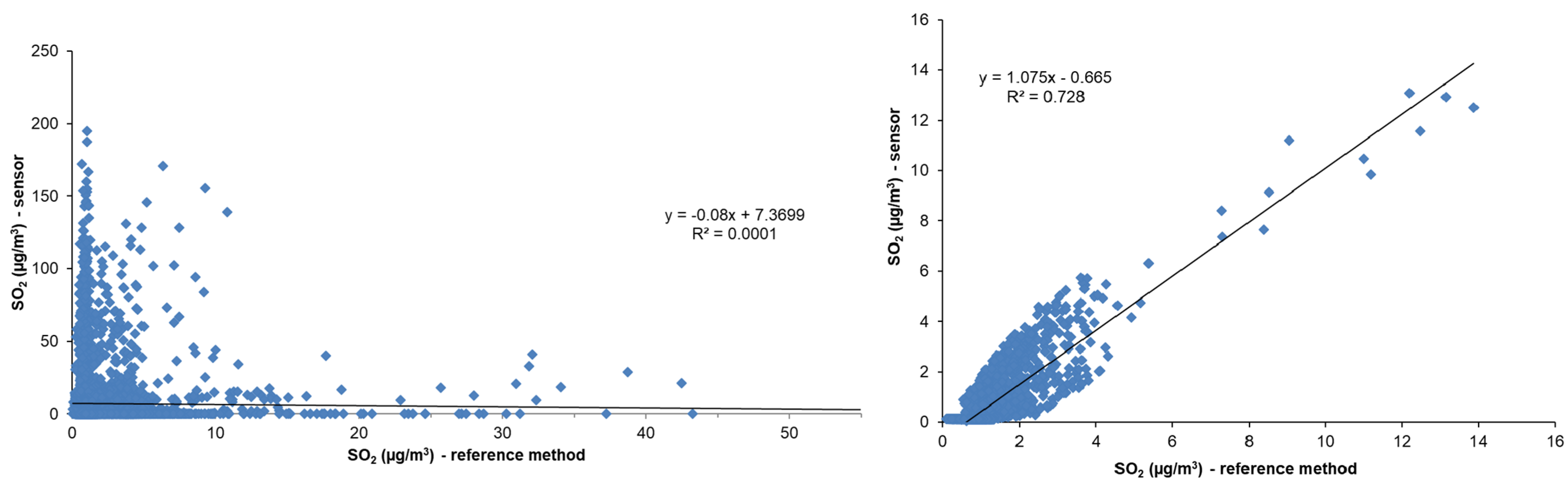
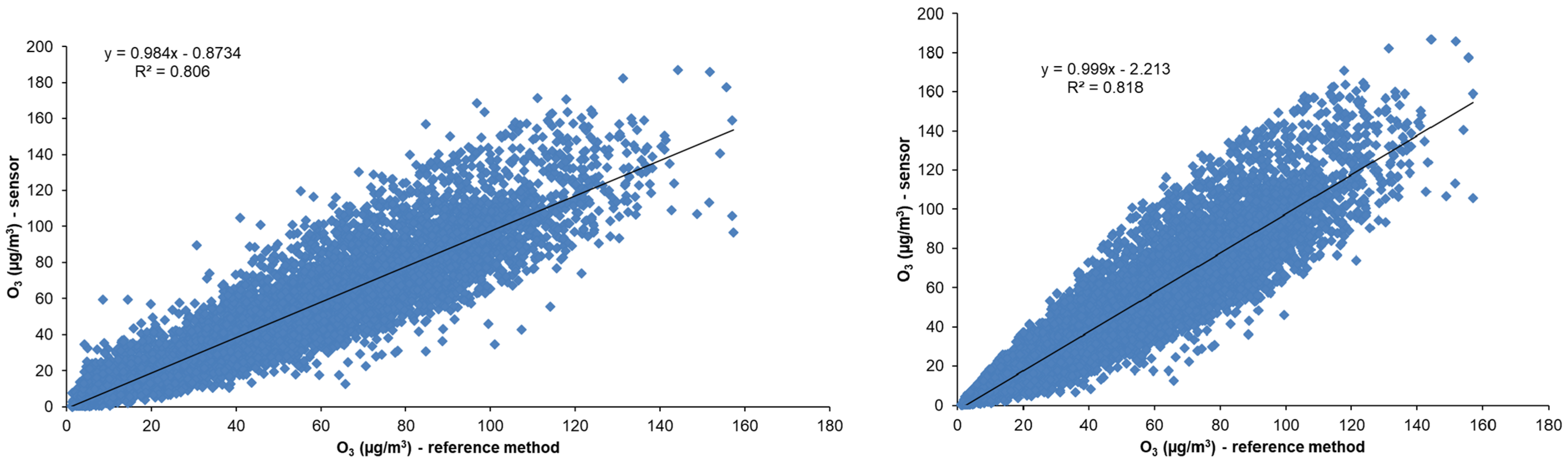
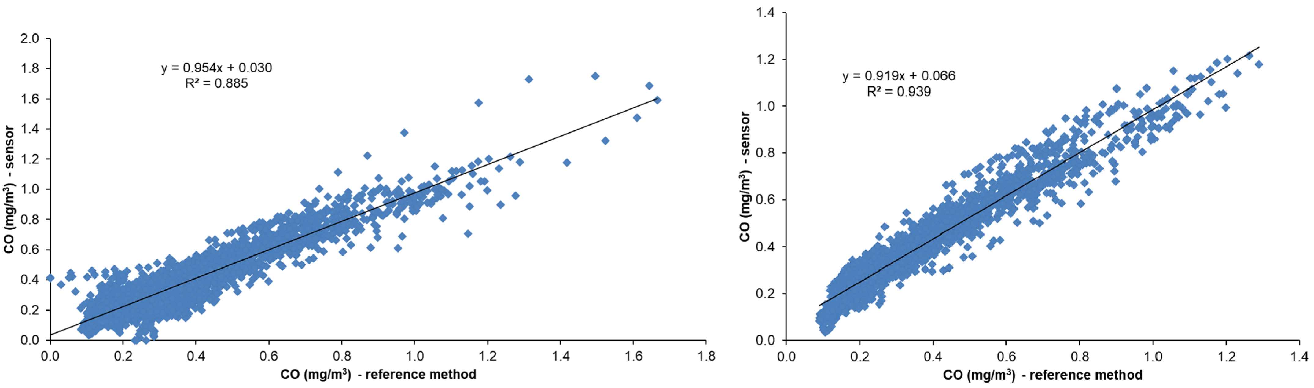
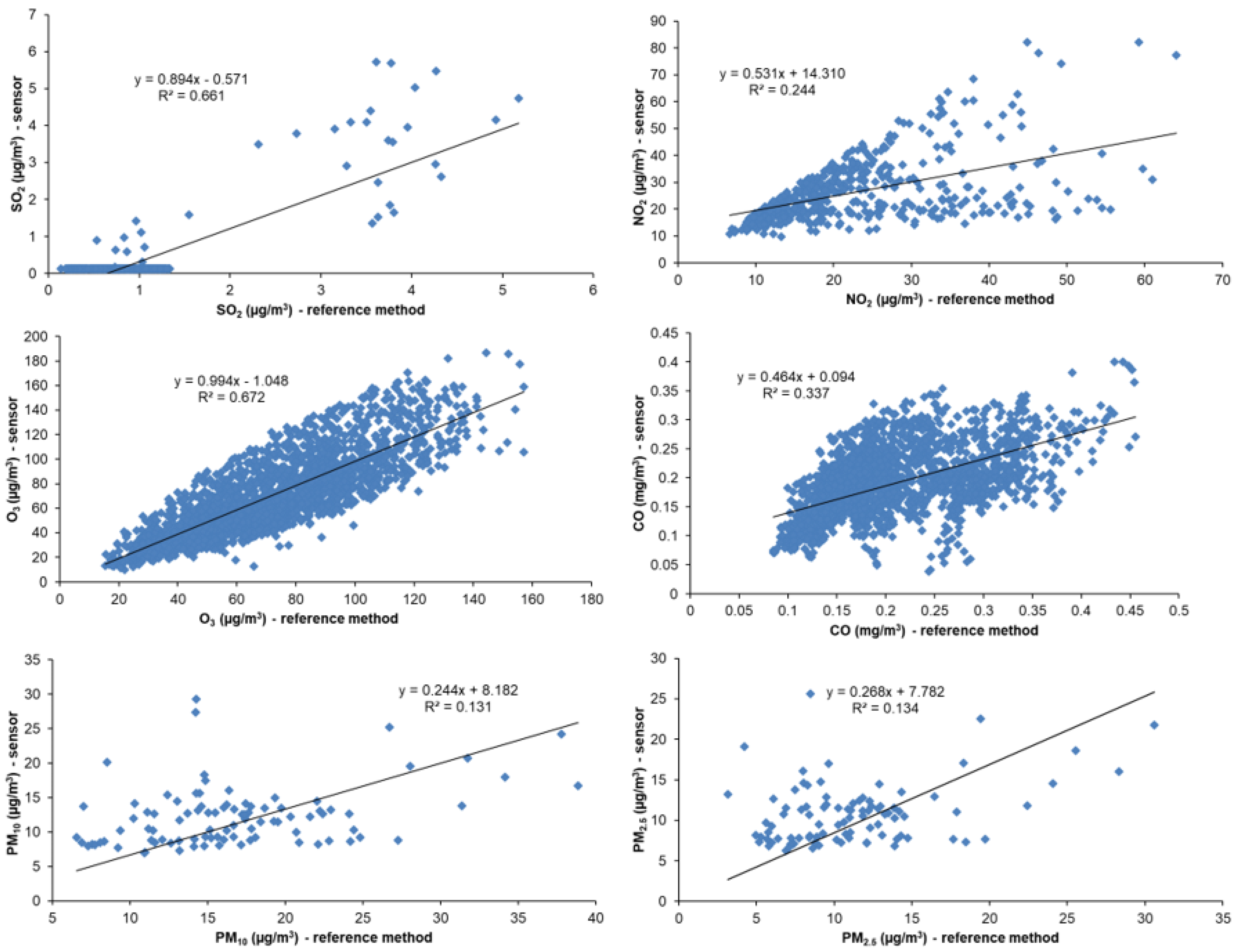
A comparison of the results obtained by sensor measurements and the results obtained by reference methods indicated that the scattering was too large for all the gaseous pollutants determined (SO₂, NO₂, O₃ and CO) (Table 2, Figure 1, Figure 2, Figure 3 and Figure 4). For this reason, data filtration was performed by rejection from further analysis of pairs of results in which the deviation between the results determined by the sensors and the results determined by the reference methods was more than 90%.

A comparison of the results determined by the sensors and the results determined by the reference methods for the PM₁₀ and PM_2.5 particulate matter fractions indicates satisfactory low scattering (Figure 5). For this reason, no data filtering was necessary, and the requirement for data coverage under the Air Protection Act [38,39,40,41] and the Air Quality Monitoring Regulation [42] was also satisfied.

In the winter part of the year, the concentration of some pollutants in the environment is higher, such as NO₂ and PM particles, while the concentration of the pollutant O₃ is lower. At low concentrations and small oscillations in temperature, the sensor for O₃ shows a better correlation with the reference method. At higher concentrations of PM particles, a good correlation with reference methods can be seen (

Table 6. Statistical significance of sensors and reference methods after filtering for winter of 2018.

Pollutant	Δ	Std (Δ)	SE (Δ)	t	r	tcrit (p = 0.95)
SO2	0.29	0.831	0.0308	9.336	0.6939	1.9630
NO2	4.5	10.26	0.305	14.8702	0.8089	1.9621
O3	5.0	7.22	0.184	27.1635	0.9605	1.9615
CO	−0.03	0.060	0.0015	19.4703	0.9557	1.9615
PM10	−12.4	10.05	1.266	9.8223	0.8860	1.9990
PM2.5	−10.8	11.14	1.278	8.4592	0.8264	1.9921

, Figure 6).

With the beginning of the warmer parts of the year, SO₂ and O₃ concentrations increase, while PM particle concentrations decrease due to the reduction in pollution sources (house heating). With the increase in concentrations, the sensor for SO₂ shows a better correlation with the reference method, while for the sensor for O₃, the correlation worsens due to the greater difference in temperatures between morning and afternoon temperatures, which has a bad effect on the sensor’s operation. The decrease in the concentration of PM particles drastically worsens the correlation (

Table 7. Statistical significance of sensors and reference methods after filtering for spring of 2018.

Pollutant	Δ	Std (Δ)	SE (Δ)	t	r	tcrit (p = 0.95)
SO2	0.76	0.421	0.0141	53.7858	0.9125	1.9626
NO2	1.7	8.20	0.292	6.0701	0.6404	1.9630
O3	−2.7	14.11	0.339	8.1528	0.8609	1.9613
CO	−0.05	0.040	0.0010	55.6158	0.7719	1.9614
PM10	1.9	8.01	0.839	2.2358	0.5436	1.9867
PM2.5	−1.5	6.40	0.667	2.2003	0.5814	1.9864

, Figure 7).

In the summer, when temperatures are highest in Zagreb, there are differences between the morning temperature when the humidity is higher and the afternoon temperature when the humidity is low but the temperature is high, and this results in the sensors showing a bad correlation. By moving into cooler parts of the year, the correlations improve for SO₂, O₃, CO and PM (

Table 8. Statistical significance of sensors and reference methods after filtering for summer of 2018.

Pollutant	Δ	Std (Δ)	SE (Δ)	t	r	tcrit (p = 0.95)
SO2	0.67	0.334	0.0109	60.9140	0.8130	1.9624
NO2	−3.6	11.57	0.550	6.5378	0.4949	1.9654
O3	1.8	18.54	0.398	4.4610	0.8188	1.9611
CO	0.01	0.061	0.0013	10.0311	0.5812	1.9611
PM10	4.5	6.39	0.659	6.8998	0.3612	1.9858
PM2.5	0.4	5.07	0.553	0.7962	0.3661	1.9858

and

Table 9. Statistical significance of sensors and reference methods after filtering for autumn of 2018.

Pollutant	Δ	Std (Δ)	SE (Δ)	t	r	tcrit (p = 0.95)
SO2	0.51	0.347	0.0177	28.9744	0.9629	1.9661
NO2	−2.1	13.0	0.454	4.719	0.7184	1.9629
O3	6.3	10.11	0.280	22.4829	0.8557	1.9618
CO	0	0.064	0.014	0.3880	0.9576	1.9611
PM10	14.7	11.34	1.223	11.9957	0.6856	1.9883
PM2.5	10.5	10.96	1.169	8.9755	0.7594	1.9876

, Figure 8).

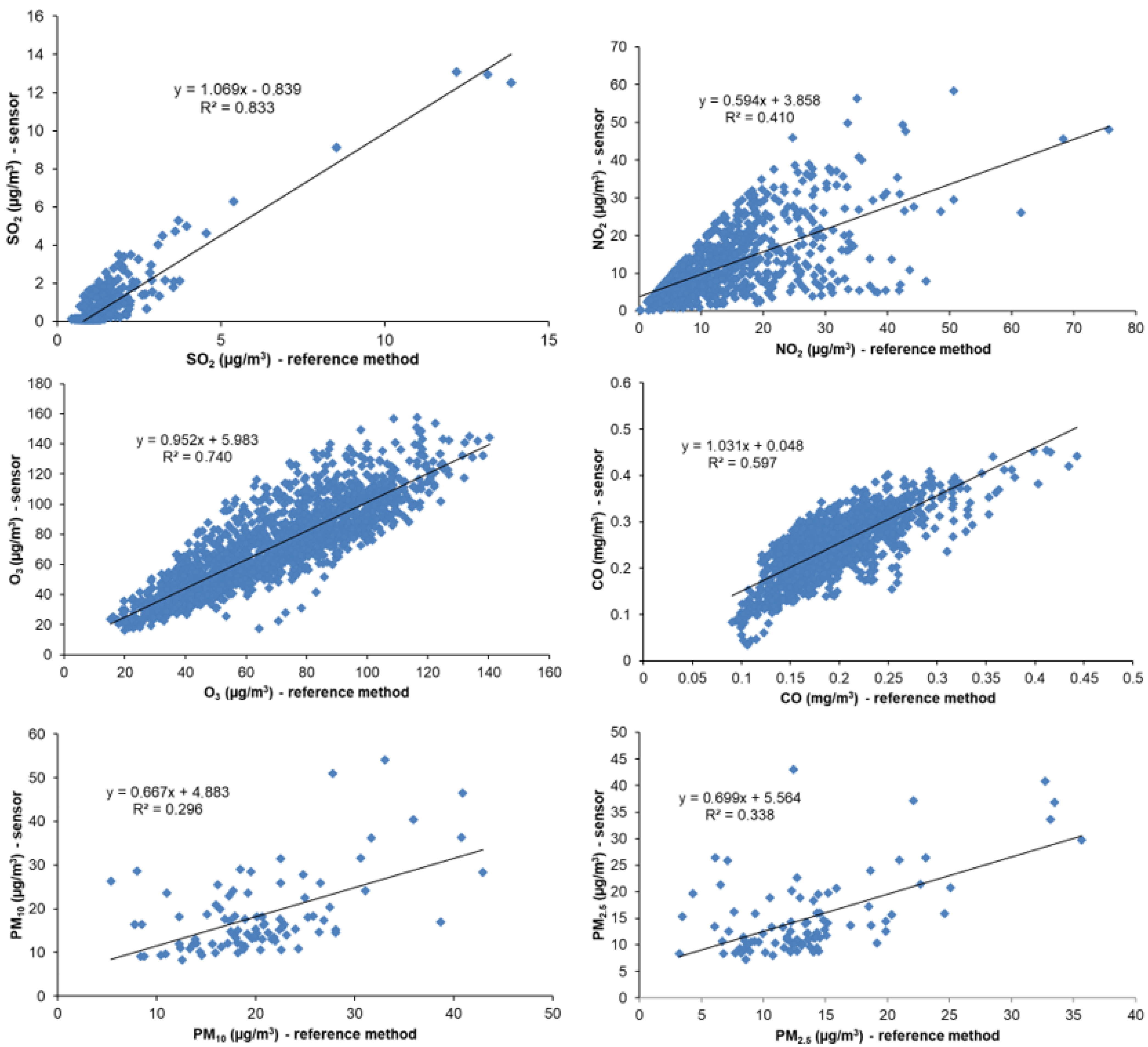
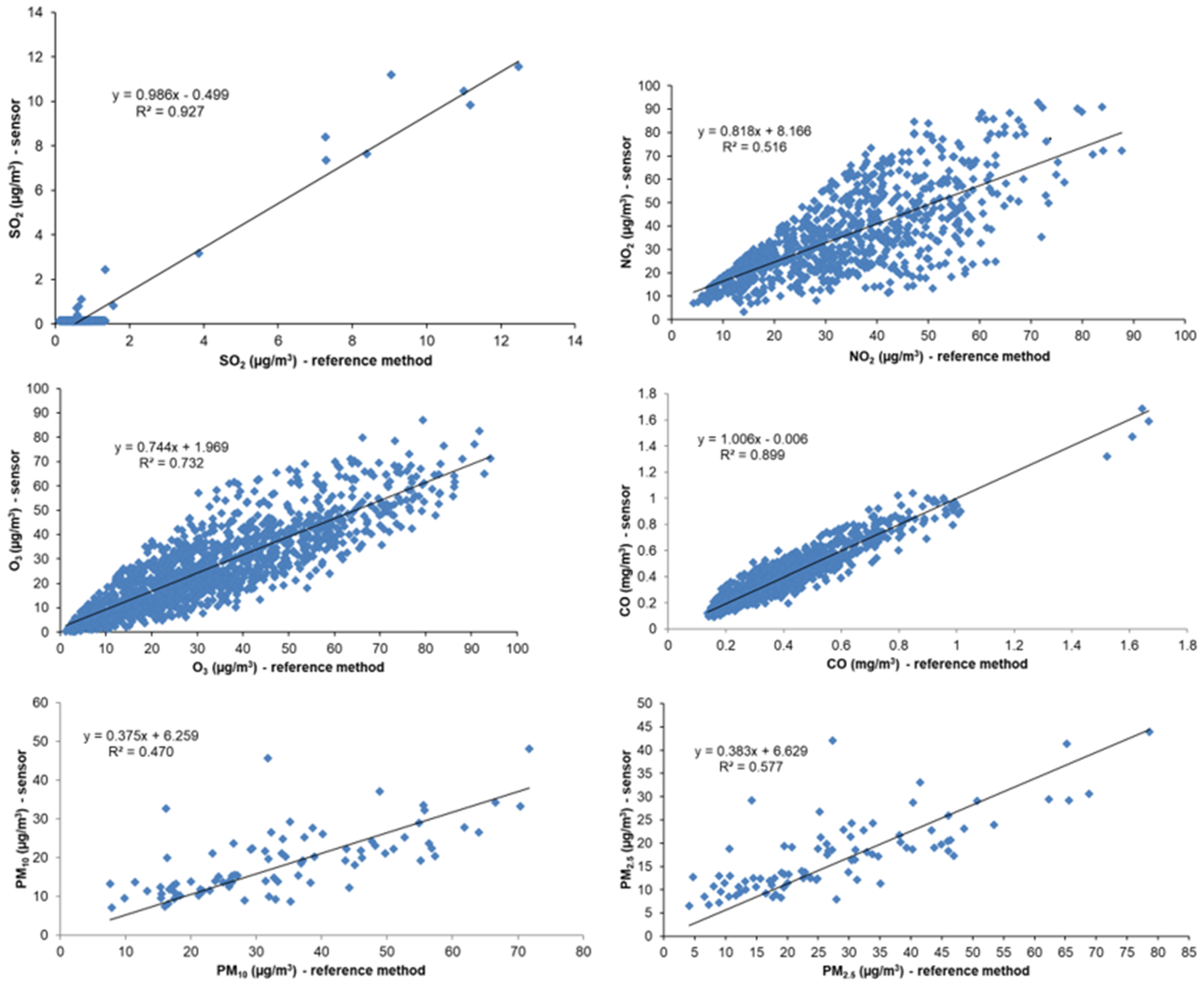
The results of the regression analysis showed a strong seasonal dependence for all pollutants. The regression analysis for SO₂, CO, PM₁₀ and PM_2.5 shows a better correlation for seasons when concentrations were increased, while for seasons when concentrations were lower the correlation between sensor and reference data is very poor. For the O₃ sensor, the correlation is better for the seasons when the concentrations are lower compared to the seasons when the concentrations are higher. For the NO₂ sensor, there is no correlation by season, nor is it related to the concentration level. Observing unfiltered data (Figure 6, Figure 7, Figure 8 and Figure 9), the highest correlation between sensors and referent methods was obtained for CO and O₃.

For sulphur dioxide (SO₂), the total data coverage for 2018 before filtering was 77.7% and, after filtering, 33.9%, which did not satisfy the criterion of data coverage. The statistics show that there was a significant statistical difference between the reference method and the sensors both for the whole year and in all seasons.

For nitrogen dioxide (NO₂), the total data coverage for the year 2018 before filtering was 77.7% and after filtering the data amounted to 38.8%, thus not meeting the criterion of data coverage in accordance with the regulations. The statistics show that there was a significant statistical difference between the reference method and the sensors both for the whole year and in all seasons.

For ozone (O₃), the total data coverage for 2018 was 81.1% and, after filtering the data, 77.8%, thus not meeting the data coverage criteria in accordance with the regulations. The statistics show that there was a significant statistical difference between the reference method and the sensors both for the whole year and in all seasons.

For carbon monoxide (CO), the total data coverage for 2018 before filtering was satisfactory (90.3%), but after filtering data it was 88.4% and thus did not meet the minimum data coverage criterion. The statistics show that there was a significant statistical difference between the reference method and the sensor, except in the fall.

For PM₁₀, the total coverage of data for 2018 was 94.5%, thus satisfying the criterion of data coverage according to the Air Protection Act and the Regulation on Air Quality Monitoring [38,39,40,41,42]. The statistics show that there was a significant statistical difference between the reference method and the sensor.

For PM_2.5, the total data coverage for 2018 was 98.9%, thus satisfying the data coverage criterion according to the Air Protection Act and the Regulation on Air Quality Monitoring [38,39,40,41,42]. The statistics show that there was no significant statistical difference between the reference method and the sensors for the whole year and summer, while in the other seasons (winter, spring and autumn) there was a statistically significant difference.

The main problem in this project is the calibration of sensors, and many papers have suggested that better results are obtained with better calibration [25,26]. Also, as said before, the first step before stating the measuring campaign is to perform field calibration, and as that calibration was not performed, the results were not so promising. But, according to many papers which oriented on the calibration of sensors, it is clear that not only field calibration before measurements is needed but also calibrations before every season of the measurements [13,30].

4. Conclusions

This study has shown that the results obtained from sensory measurement techniques are highly seasonally dependent, suggesting the sensitivity of meteorological conditions to the measurement technique. Seasonal dependence, as well as poor data coverage due to failures (especially in the determination of SO₂, NO₂ and O₃) and wastefulness of the results, call into question their application in the continuous monitoring of air quality. The best agreement with the reference method was shown by CO sensors and the PM_2.5 particulate matter fractions, while the PM₁₀ and PM_2.5 sensors showed the least scatter and satisfactory data coverage. The results also indicate the need to make calibrations at the measurement site before starting the measurement campaign itself. The calibration was not performed in the field, but a factory calibration was used, which was found to be insufficient.

This study indicates that the use of factory calibration is not sufficient to obtain high-quality measurements by sensors and that seasonal calibration is needed. Factory calibrations show good calibration at higher concentrations for most pollutants except for O₃, but such calibration turned out to be very poor at low concentrations of most pollutant parameters except for O₃. The experiment shows the need for field calibration at least for warmer and colder parts of the year, although field calibration for each season would be better. Future research will focus on improving seasonal calibrations using calibration chambers for gaseous sensors and field calibrations for PM sensors. It is also necessary to examine the transfer of calibrations to different types of stations, which was attempted in some experimental measurements [13,30]. Today’s use of artificial intelligence (machine learning and neural networks) can greatly help in better calibration of sensors for specific climate conditions.

Today’s policy of the European Union, influenced by AQUIL-a and reference laboratories of the European Union, is to get better control of the use and calibration of sensors. Within a few years, the plan is to pass legislation related to sensor calibration. This is why it is essential to research better calibration methods using newer tools in the field of measurements and computer science.