Abstract
Understanding how traffic contributes to air pollution, especially in urban areas, is essential for designing effective strategies to reduce air pollution emissions. This study examines the hourly association between traffic volume and concentrations of two air pollution indicators (NO2 and PM10) using high-resolution data from two monitoring stations in Helsinki. A Prophet time series model was applied to forecast hourly traffic trends for 2024, which were then compared to yearly average NO2 and PM10 concentrations. Polynomial regression and cross-correlation analyses were used to capture temporal patterns and assess the strength and timing of the relationship. The results show a strong alignment between traffic and NO2 and PM10 concentrations, particularly at the traffic-heavy measuring site (Mäkelänkatu supersite), with minimal time lag observed. Root mean square error (RMSE) and polynomial fit comparisons confirmed the predictive value of traffic trends in estimating the behavior of NO2 and PM10 concentrations. These findings support the use of traffic-based proxy models as practical tools for real-time air pollution assessment and for informing targeted urban air quality interventions.
1. Introduction
Motor vehicles are among the primary contributors to urban air pollution, particularly in developed regions where high traffic densities and reliance on internal combustion engines continue to dominate transportation systems [1,2,3]. The expansion of motorized vehicle fleets, combined with the proximity of emissions to densely populated areas, has made traffic-related pollution a main environmental and public health issue [4,5]. Traffic emissions, especially nitrogen oxides (NOx) and particulate matter (PM2.5 and PM10), are known to negatively affect human health. People living close to busy roads are particularly exposed to higher concentrations of these pollutants. Studies have shown associations between long-term exposure and increased risk of respiratory diseases such as asthma, chronic bronchitis, and reduced lung function, as well as cardiovascular problems including high blood pressure and heart disease. There is also growing evidence that regular exposure to traffic-related air pollution contributes to premature mortality. These health effects underline the importance of monitoring traffic emissions and understanding their patterns over time [6,7,8,9]. Unlike industrial or residential emissions (e.g., heating), which can be regulated at point sources, vehicle emissions are more challenging to control due to their widespread distribution and continuous nature [10]. Although regulations such as the European emission standards (Euro 4, 5, and 6) have introduced stricter limits on vehicle exhaust pollutants like NOx and PM, the real-world effectiveness of these standards often varies depending on vehicle maintenance, driving behavior, and urban traffic conditions [11,12,13,14,15]. Moreover, even newer Euro 6 vehicles can contribute significantly to urban pollution during congestion or cold-start conditions [16]. Additionally, variations in fleet composition—such as the prevalence of diesel-powered trucks versus petrol-driven passenger cars—result in complex emission profiles that differ in terms of nitrogen oxides, particulate matter, carbon monoxide (CO), and volatile organic compounds (VOCs). Old diesel vehicles, in particular, emit higher levels of NOx and fine particulates, exacerbating urban air quality problems [17,18,19,20]. In response, several European cities have implemented low-emission zones (LEZs) or outright diesel vehicle bans, particularly targeting older Euro 4 and Euro 5 models. Cities have restricted or phased out diesel vehicles in central areas to comply with EU air quality directives and reduce public exposure to harmful pollutants [21,22,23]. These policies reflect growing recognition of the disproportionate contribution of diesel emissions to urban air pollution, especially during peak traffic periods. In recent years, the City of Helsinki has introduced several policies to reduce traffic-related air pollution, with a particular focus on diesel emissions. These include restrictions on the use of heavy-duty vehicles in specific zones, financial incentives for low-emission transport, and infrastructure investments to support electric vehicles and public transportation. Helsinki’s “Carbon-neutral Helsinki 2035” strategy outlines further steps to phase out fossil fuel-powered traffic and reduce air pollution exposure in densely populated areas [24].
Accurate assessment of traffic-related pollution at the local scale remains challenging due to limited spatial resolution in conventional air quality models and satellite-based instruments. While models such as Chemistry-Transport Models (CTM) and Land Use Regression (LUR) can incorporate traffic data, they often rely on coarse spatial assumptions and may not reflect short-term variations in traffic flow [25,26,27,28,29]. Data-driven approaches, using direct measurements and time-based surrogates, offer an alternative for capturing high-resolution temporal patterns [30]. These methods leverage seasonality, daily patterns, and statistical modeling (e.g., ARIMA, Prophet) to infer pollutant behavior and trends, especially when detailed emission inventories are not available [31,32].
In reality, urban traffic flow fluctuates significantly throughout the day due to commuting patterns, road network structures, and external factors such as weather or traffic incidents [33]. This temporal variability shows the need for precise models that can predict traffic volume with high temporal resolution. Given the nature of traffic, heating, and other anthropogenic emission sources, using time as a surrogate variable can be problematic. While temporal patterns such as rush hours or heating seasons do correlate with emission events, they are only proxies and may not accurately capture the underlying emission scenarios in all contexts. For instance, the same time of day may correspond to very different emission intensities depending on weather conditions, holiday schedules, or regional infrastructure. Therefore, it is essential to refine these surrogate variables through proxy models that incorporate contextual information.
The objective of this study is to evaluate whether modeled hourly traffic patterns can serve as reliable predictors of traffic-related air pollutant concentrations (NO2 and PM10) at urban monitoring sites. It also enables discussion of the potential use of air pollutant concentrations as indirect proxies for traffic in reverse scenarios, especially in locations lacking detailed traffic monitoring. This study models hourly traffic volume using a time series forecasting approach (Prophet), followed by polynomial fitting to describe typical diurnal traffic patterns. Unlike methods that rely on static or aggregated traffic data, this approach captures the dynamic nature of urban traffic flow. The resulting polynomial functions provide a compact and transferable representation of daily traffic variation, which can be used as surrogate input in air quality models to estimate exposure to traffic-related emissions with higher temporal resolution. Beyond air pollution research, these functions can support urban planning, transport engineering, and policy evaluation by offering interpretable patterns that reflect typical congestion periods and emission peaks.
2. Materials and Methods
This study was conducted in Helsinki, Finland, where air pollution data was collected from two air quality monitoring stations (Mäkelänkatu supersite and Kallio) and traffic volume data were obtained from multiple traffic measurement points. The geographical locations of these stations are presented in Figure 1. The data were processed and analyzed using Python programming language (v3.12, www.python.org, accessed on 10 March 2025) in the Spyder environment. Key libraries included pandas for data manipulation, numpy for numerical computations and polynomial modeling, matplotlib and seaborn for visualization, scikit-learn for regression and evaluation metrics, and Prophet for time-series forecasting [34,35].
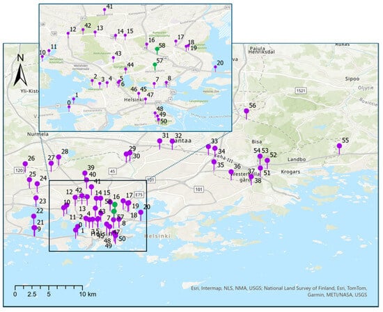
Figure 1.
Air quality (57-Kallio, 58-Mäkelänkatu) and traffic counting stations.
The air pollution measurements were conducted by the Helsinki Region Environmental Services Authority (HSY) at two fixed monitoring stations, strategically positioned to capture representative urban air quality conditions. The Mäkelänkatu supersite station is located at a busy traffic site, and Kallio is an urban background station influenced by surrounding traffic [36]. These stations continuously measured key air pollutants, including NO, NO2, PM10, PM2.5, O3, black carbon (BC), and particle number concentration (PNC), using reference-grade instruments in compliance with EU monitoring standards [36]. The hourly mean data was selected, ensuring comprehensive temporal coverage of pollution levels. Traffic data for this study were obtained from the Helsinki Region Infoshare (HRI) Open Data Portal, specifically from the dataset titled “Traffic Volumes in Helsinki” (https://hri.fi/data/en_GB/dataset/liikennemaarat-helsingissa, accessed on 13 March 2025). The maintainer of the dataset is the City of Helsinki. Traffic volume data were obtained from 56 automatic traffic measurement stations distributed across the study area and were downloaded from the Helsinki Region Infoshare service on 16 March 2025, under the Creative Commons Attribution 4.0 license. The primary parameters recorded included the total number of vehicles and different vehicle categories, which were later analyzed for their potential impact on air pollution levels. However, it is important to note that the dataset does not include full-year or full-week traffic measurements. The traffic volumes represent average values derived from Monday to Thursday during September and October each year. As such, the dataset reflects typical weekday traffic, while weekend data is not available. A more detailed comparison between weekdays and weekends, as well as seasonal variability, will be addressed in future research using continuous time-series data.
All datasets were preprocessed to ensure consistency and comparability. The air quality data were quality-checked for missing values and potential anomalies. Hourly traffic averages were computed for each year from 2010 to 2023 to capture daily fluctuations. Prophet, an advanced time-series forecasting model, was employed to predict hourly traffic volume for 2024 based on historical trends from 2019–2023 [37,38]. Prophet is an additive model that decomposes time series into trend, seasonality (daily, weekly, and yearly), and holiday effects. It is robust for missing data and outliers and automatically detects changepoints in the trend, making it well-suited for irregular real-world data such as traffic volumes [39,40,41,42]. The model input consisted of aggregated hourly traffic counts from all available measurement stations in Helsinki. Rather than training separate models per station, the traffic variable was first summed across all sites, creating a unified time series representing city-level traffic flow. This aggregated approach was chosen to capture overall traffic seasonality and diurnal structure, which could then be related to pollutant concentrations at specific stations. The model incorporated daily and weekly seasonality components and was trained in a multiplicative mode. To ensure that the predicted 2024 traffic volumes aligned with recent observed trends, a post-processing scaling factor was applied to the forecasted values. This factor was computed as the ratio of the multi-year average hourly traffic volume (2019–2023) to the average hourly traffic in 2023. The adjustment preserved the seasonality and diurnal pattern produced by Prophet, while aligning the forecast magnitude with the recent multi-year baseline. The predicted traffic for 2024 was then compared to historical trends, and all data were visualized in a combined plot to assess their consistency. To compare the temporal structure of the Prophet prediction, we fitted a polynomial function to the predicted hourly 2024 traffic values. Several polynomial degrees (from 6 to 10) were tested, and the 9th-degree polynomial provided the best compromise between capturing the dual-peak structure and avoiding unrealistic oscillations. The model was fitted using least squares regression. This approach was used solely for smooth approximation and visualization, not for prediction. To assess relationships between traffic and air pollutants (NO2 and PM10), additional statistical analyses were performed, including root mean square error (RMSE) to quantify model fit, linear regression to estimate direct relationships, and cross-correlation to evaluate temporal alignment between pollutant levels and traffic patterns.
3. Results and Discussion
The analysis of traffic data began with processing and aggregating hourly vehicle counts to examine long-term trends and daily fluctuations across different years. Figure 2 presents the hourly average traffic volume across all measurement stations from 2010 to 2023, revealing a consistent bimodal daily pattern with morning and afternoon peaks, corresponding to commuting hours. Traffic volume increases sharply from 05:00, reaching a morning peak between 07:00 and 09:00, reflecting the morning traffic rush hours. A second peak occurs between 15:00 and 18:00, reflecting the afternoon traffic rush hours. The afternoon peak appears slightly broader, indicating a more gradual dispersal of traffic. Nighttime and early morning hours (00:00–05:00) show the lowest traffic levels.
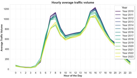
Figure 2.
Hourly average traffic volume across all measuring stations for years 2010 to 2023 (Monday–Thursday, September–October each year).
While overall patterns remain stable across the years, a gradual decrease in peak-hour traffic is observed, particularly in recent years, which may reflect efforts to reduce vehicle dependence, promote sustainable transportation, and increase public awareness of traffic-related pollution. During the years 2020 and 2021, the clear drop in traffic volumes was caused by COVID-19 restrictions [43]. The traffic volumes have also remained lower in 2022–2023, since remote working has become more common, and this has reduced mobility.
The 2024 predicted traffic (Figure 3), shown as a red dashed line, generally follows the expected diurnal pattern observed across previous years. It successfully captures both the morning and afternoon peak traffic periods, with peak timings aligning well with historical data. However, the 2024 morning peak appears slightly overestimated relative to recent years, particularly during hours 7–9. This likely results from Prophet’s reliance on historical average seasonal patterns, which may emphasize earlier years where the morning peak was stronger. As a ML-based time series model, Prophet uses decomposable components—trend, seasonality, and changepoints—learned from past data. However, it does not dynamically adjust for year-to-year behavioral shifts (e.g., remote work, school hours), so localized overestimation can occur in time windows with sharper traffic peaks. Prophet models seasonality using a Fourier series representation, which smooths over the full training period. As such, it may amplify older peak patterns if recent deviations are not strong enough to shift the estimated seasonal components. This deviation may reflect the inherent uncertainty in extrapolating future traffic behavior or the limitations of the model. Despite these differences, the overall alignment indicates that the forecasting model effectively captures the dominant seasonal traffic patterns. Future refinements could involve incorporating additional external variables, such as weather conditions (e.g., precipitation, temperature), public holidays, and public transport usage, which are known to influence daily traffic patterns in Helsinki. These could be integrated into the modeling framework as regressors to improve prediction accuracy and account for external variability. Moreover, extending the analysis to compare urban and rural (or less traffic-exposed) sites could help evaluate the spatial generalizability of the model and better understand location-specific traffic–pollution dynamics.
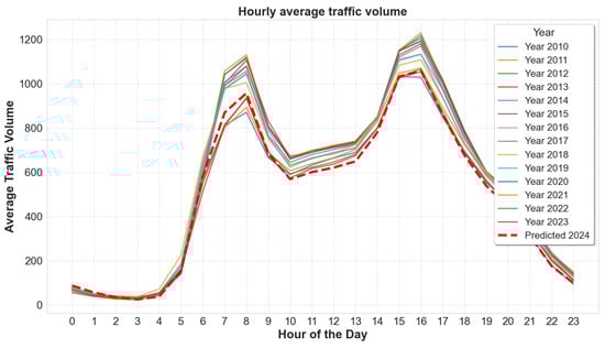
Figure 3.
Hourly average traffic volume for all measuring stations with prediction for 2024 (Monday–Thursday, September–October each year).
Figure 4 illustrates the comparison between hourly average traffic values predicted by the Prophet model (blue dots) and a fitted 9th-degree polynomial function (red line) based on the same data. The polynomial fit closely follows the overall structure of the predicted traffic, effectively capturing both the morning and evening peak hours. Compared to the original Prophet output, the polynomial provides a smoother representation, particularly in transitional periods such as midday and evening. Despite minor deviations, the close alignment demonstrates that polynomial interpolation—especially with rounded coefficients—can serve as a computationally efficient and interpretable approximation of Prophet’s predictions for capturing daily traffic dynamics in 2024.
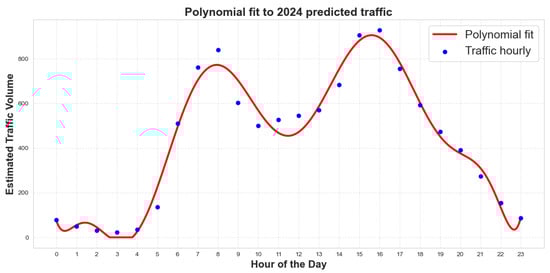
Figure 4.
Polynomial estimation for traffic prediction.
The following equation represents the 9th-degree polynomial function fitted to the Prophet-predicted hourly traffic data for a 31-day prediction period for 2024:
where y represents the estimated traffic volume and x is the hour of the day.
y = 0.0000004480x9 − 0.0000992510x8 − 0.0069570963x7 − 0.2345560814x6 + 4.3175397657x5
− 44.4978440597x4 + 244.7426228105x3 − 615.8006568175x2 + 505.4296359966x + 51.4997991675
− 44.4978440597x4 + 244.7426228105x3 − 615.8006568175x2 + 505.4296359966x + 51.4997991675
The coefficients determine how much each term influences the final traffic volume. Due to the sensitivity of high-degree polynomial functions to coefficient rounding, coefficients were kept at higher precision to ensure the plotted curve accurately follows the fitted traffic pattern. To assess the robustness of the polynomial coefficients, standard errors were calculated using the covariance matrix from the least squares regression. Mid-order terms (e.g., x3 to x6) showed relatively low standard errors, while the highest-order terms and intercept exhibited higher uncertainty, as expected. To further test sensitivity, bootstrap resampling (1000 iterations) was used. This analysis confirmed the same pattern: moderate variability in core terms and greater spread in high-order or constant terms. While the overall curve shape remained stable across resamples, high-degree polynomial fits may suffer from numerical sensitivity. Future models could benefit from more stable smoothing methods such as splines or regularized regressions.
The hourly pollutant trends (Figure 5) indicate a strong influence of traffic emissions, particularly in Mäkelänkatu station, where NO2 and BC concentrations show distinct morning (6–10 A.M.) and evening (4–8 P.M.) peaks, aligning with rush hours. Kallio exhibits a similar but less pronounced pattern, suggesting lower traffic density. PM2.5 levels are generally stable, with slight increases during peak hours, indicating contributions from both traffic and background sources. PM10 concentrations display a peak during morning hours at Mäkelänkatu, likely due to a combination of exhaust and non-exhaust traffic-related emissions, including road dust and tire wear. At Kallio, PM10 levels remain lower and show less variability, further confirming the difference in local traffic exposure between the two stations. Overall, the patterns confirm that Mäkelänkatu station has stronger traffic-related pollution, while Kallio, though affected, shows lower overall pollutant levels.
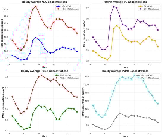
Figure 5.
Daily variation of annual mean concentrations in 2024, at two measuring stations.
Traffic conditions at the two monitoring stations differ notably in both volume and character. Mäkelänkatu station is located adjacent to a major arterial road, which serves as a key north–south connector in Helsinki and carries a high volume of commuter traffic, including buses and heavy-duty vehicles. In contrast, Kallio station is situated in a more residential neighborhood, near smaller collector roads with lower vehicle counts and reduced heavy vehicle presence. The distance between the monitoring stations and the nearest road is also shorter at Mäkelänkatu (~1 m) than at Kallio (~60 m), which likely amplifies the measured impact of local emissions. These traffic-related differences help explain the observed pollutant patterns in Figure 5 and Figure 6, including the sharper NO2 and BC peaks at Mäkelänkatu and the flatter curves at Kallio.
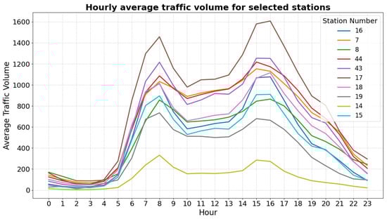
Figure 6.
Hourly average traffic volume at 10 traffic measurement stations nearest to the air quality monitoring stations (figure for all station is in Appendix A).
Figure 6 presents the hourly average traffic volumes for 10 selected traffic measurement stations located closest to the air quality monitoring sites. The figure shows a clear variation in traffic intensities across these stations. While some stations show distinct peak volumes during morning and evening hours, others exhibit more moderate patterns throughout the day. Importantly, the traffic stations located near Mäkelänkatu and Kallio show mid-range traffic levels compared to the other selected sites. This supports the approach of using averaged traffic profiles for modeling and pollutant comparisons, ensuring that the results are representative of typical local conditions rather than being overly influenced by extreme traffic sites. For reference, a complete figure showing hourly average traffic volumes for all available stations is provided in Appendix A (Figure A1).
To further quantify the relationship between traffic and pollution levels, hourly averaged pollutant concentrations (NO2 and PM10) were compared with traffic volume predictions derived from Prophet modeling (Figure 7). All variables were normalized to a 0–1 scale to allow direct comparison of hourly trends. The scaled profiles reveal a strong temporal alignment between traffic intensity and NO2/PM10 concentrations at both stations. The rise in traffic during morning hours (6–10 a.m.) corresponds to elevated NO2 and PM10 levels, especially at Mäkelänkatu station, supporting the interpretation that traffic is a major contributor there. Afternoon and evening patterns show a delayed response in pollutant levels, possibly due to meteorological conditions, secondary formation, or sustained emissions during slower-moving traffic [44,45,46,47]. Kallio station shows the same general trend but with lower peak intensities, again consistent with lower traffic influence. These comparisons support the findings from earlier hourly trends and suggest that traffic dynamics can be a reliable predictor of urban pollution, particularly for NO2 and PM10, making them useful for exposure assessment and traffic regulation strategies.
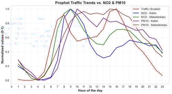
Figure 7.
Comparison of scaled Prophet traffic trends and pollutants. All values were normalized (scaled 0–1) to allow comparison of trends.
To quantify the similarity between traffic volume and pollutant patterns, polynomial-fitted trends were compared using RMSE (Table 1). The strongest alignment was observed for NO2 at Mäkelänkatu station (RMSE = 0.1982), supporting its proximity to traffic emissions. Kallio showed a slightly weaker relationship (RMSE = 0.3002), consistent with its lower traffic exposure. PM10 trends followed a similar pattern, with better correlation at Mäkelänkatu (RMSE = 0.2402) than at Kallio (RMSE = 0.2864), likely reflecting the combination of traffic and other sources (e.g., regional background). Results were further supported by R2 values, which indicated stronger shared variability between traffic and pollutant trends at Mäkelänkatu (R2 = 0.4843 for NO2, 0.4995 for PM10) than at Kallio (R2 = 0.2073 for NO2, 0.1730 for PM10).

Table 1.
Root mean square error (RMSE) and coefficient of determination (R2) between polynomial-fitted traffic volume trends and hourly pollutant concentrations at Mäkelänkatu (traffic-influenced) and Kallio (urban background) stations.
These findings show the importance of site-specific data when modeling air quality impacts from traffic, particularly in areas with different exposure profiles and background pollution influences. In addition to regulatory-grade monitoring, low-cost sensor technologies have gained traction as a scalable solution for fine-scale air quality assessment. In Finland, pilot deployments in Helsinki and other cities have evaluated the performance of low-cost sensors for PM and NO2 under northern climate conditions. These devices, when properly calibrated or co-located with reference instruments, can provide valuable spatial resolution and capture local emissions near traffic corridors. Their affordability and ease of deployment also make them particularly suitable for expanding air pollution monitoring in developing cities, where traditional infrastructure may be limited [48,49,50].
A key limitation of this study is the lack of seasonal correction; the analysis focused on identifying general daily patterns without distinguishing between summer and winter conditions. As pollutant behavior can vary significantly by season (e.g., higher NO2 during cold months due to increased heating emissions), results may not fully capture season-specific dynamics. Future work could include stratified modeling by season or introduce seasonal dummy variables into the forecasting models to better reflect temporal variation in pollutant behavior. Additionally, the study relied on a limited number of monitoring stations. The aim is to conduct a more detailed analysis by including additional variables and expanding the number of stations to better capture spatial and temporal variability. Incorporating data from street-level sensors, meteorological conditions (e.g., wind speed, temperature inversions), and policy or traffic restriction timelines could improve model performance. Traffic behavior also varies between weekdays and weekends, and future models could benefit from day-type segmentation or explicit weekday/weekend indicators to better capture this variability. From a methodological perspective, the use of hybrid models (e.g., combining Prophet with machine learning or spatial regression) may also help capture complex interactions between traffic and air pollution, especially in heterogeneous urban environments.
4. Conclusions
This study investigated the relationship between hourly traffic volume and concentrations of NO2 and PM10 at two urban monitoring stations in Helsinki: Kallio and Mäkelänkatu. A Prophet time series model was used to forecast 2024 hourly traffic trends, which were then compared with yearly average pollutant concentrations. The analysis revealed that pollutant levels, particularly NO2, closely follow the diurnal traffic pattern, with clear peaks during morning and evening rush hours, especially at Mäkelänkatu. Polynomial fitting and RMSE evaluation confirmed a stronger association between traffic and pollutant levels at Mäkelänkatu compared to Kallio, indicating higher traffic density and direct exposure. Cross-correlation analysis showed minimal time lag between traffic volume and pollutant concentrations, further supporting traffic as a dominant emission source. Kallio exhibited a flatter trend and weaker correlation, suggesting a greater contribution from background or non-traffic sources. These findings highlight the significance of high-resolution traffic data for interpreting urban air quality dynamics and underline the importance of site-specific strategies in pollution mitigation. Future work will focus on incorporating additional variables such as weather, seasonality, and day-type indicators to improve model accuracy, as well as expanding the analysis to a broader network of monitoring stations and pollutant types. From a methodological perspective, applying hybrid models or machine learning approaches may offer further improvements in capturing nonlinear and site-specific dynamics. In addition to technical advancements, this research contributes to broader urban sustainability goals. Understanding traffic’s influence on air quality is important for improving livability, as it directly impacts residents’ health, urban noise levels, and the overall environmental quality [51,52,53]. Aligning transportation and pollution mitigation strategies supports the development of healthier, more sustainable cities, in line with initiatives such as Helsinki’s Carbon Neutral 2030 Plan and broader European Green Deal goals [24,54]. Future research should further explore how traffic modeling can inform integrated urban planning, promoting not only pollution reduction but also healthier and more sustainable urban environments.
Author Contributions
Conceptualization, N.R., T.H. and M.L.; Data curation, T.H., H.P. and J.V.N.; Formal analysis, N.R.; Investigation, N.R. and V.P.; Methodology, N.R. and M.L.; Resources, F.M.; Software, N.R. and V.P.; Supervision, T.H., F.M. and M.L.; Visualization, N.R.; Writing—original draft, N.R.; Writing—review & editing, T.H., F.M., J.V.N. and M.L. All authors have read and agreed to the published version of the manuscript.
Funding
This study was performed using the facilities and equipment funded within the European Regional Development Fund project KK.01.1.1.02.0007 “Research and Education Centre of Environmental Health and Radiation Protection—Reconstruction and Expansion of the Institute for Medical Research and Occupational Health”, and funded by the European Union—Next Generation EU (Program Contract of 8 December 2023, Class: 643-02/23-01/00016, Reg. no. 533-03-23-0006)-EnvironPollutHealth. ML is supported by Horizon Europe (URBREATH project #101139711) and European Union—Next Generation EU, grant number IA-INT-2024 (BioAntroPop) granted to the Institute for Anthropological Research, Zagreb, Croatia.
Institutional Review Board Statement
Not applicable.
Informed Consent Statement
Not applicable.
Data Availability Statement
The data that support the findings of this study are available from the corresponding author, [M.L.], upon reasonable request.
Conflicts of Interest
Author Valentino Petrić was employed by the company Ascalia d.o.o. The remaining authors declare that the research was conducted in the absence of any commercial or financial relationships that could be construed as a potential conflict of interest.
Appendix A

Figure A1.
Hourly average traffic volume at all traffic measurement stations.
References
- Borrego, C.; Tchepel, O.; Costa, A.; Martins, H.; Ferreira, J.; Miranda, A. Traffic-related particulate air pollution exposure in urban areas. Atmos. Environ. 2006, 40, 7205–7214. [Google Scholar] [CrossRef]
- Han, X.; Naeher, L.P. A review of traffic-related air pollution exposure assessment studies in the developing world. Environ. Int. 2006, 32, 106–120. [Google Scholar] [CrossRef]
- Harrison, R.M.; Vu, T.V.; Jafar, H.; Shi, Z. More mileage in reducing urban air pollution from road traffic. Environ. Int. 2021, 149, 106329. [Google Scholar] [CrossRef] [PubMed]
- Khreis, H. Traffic, air pollution, and health. In Advances in Transportation and Health; Elsevier: Amsterdam, The Netherlands, 2020; pp. 59–104. ISBN 978-0-12-819136-1. [Google Scholar]
- Laumbach, R.J.; Kipen, H.M. Respiratory health effects of air pollution: Update on biomass smoke and traffic pollution. J. Allergy Clin. Immunol. 2012, 129, 3–11. [Google Scholar] [CrossRef] [PubMed]
- Boogaard, H.; Patton, A.P.; Atkinson, R.W.; Brook, J.R.; Chang, H.H.; Crouse, D.L.; Fussell, J.C.; Hoek, G.; Hoffmann, B.; Kappeler, R.; et al. Long-term exposure to traffic-related air pollution and selected health outcomes: A systematic review and meta-analysis. Environ. Int. 2022, 164, 107262. [Google Scholar] [CrossRef] [PubMed]
- Fussell, J.C.; Franklin, M.; Green, D.C.; Gustafsson, M.; Harrison, R.M.; Hicks, W.; Kelly, F.J.; Kishta, F.; Miller, M.R.; Mudway, I.S.; et al. A Review of Road Traffic-Derived Non-Exhaust Particles: Emissions, Physicochemical Characteristics, Health Risks, and Mitigation Measures. Environ. Sci. Technol. 2022, 56, 6813–6835. [Google Scholar] [CrossRef]
- Mak, H.W.L.; Ng, D.C.Y. Spatial and Socio-Classification of Traffic Pollutant Emissions and Associated Mortality Rates in High-Density Hong Kong via Improved Data Analytic Approaches. Int. J. Environ. Res. Public Health 2021, 18, 6532. [Google Scholar] [CrossRef]
- Zhang, K.; Batterman, S. Air pollution and health risks due to vehicle traffic. Sci. Total Environ. 2013, 450–451, 307–316. [Google Scholar] [CrossRef]
- Batterman, S.; Chambliss, S.; Isakov, V. Spatial resolution requirements for traffic-related air pollutant exposure evaluations. Atmos. Environ. 2014, 94, 518–528. [Google Scholar] [CrossRef]
- Ghadiri, Z.; Rashidi, Y.; Broomandi, P. Evaluation Euro IV of effectiveness in transportation systems of Tehran on air quality: Application of IVE model. Pollution 2017, 3, 639–653. [Google Scholar] [CrossRef]
- Liu, Y.; Martinet, S.; Louis, C.; Pasquier, A.; Tassel, P.; Perret, P. Emission Characterization of In-Use Diesel and Gasoline Euro 4 to Euro 6 Passenger Cars Tested on Chassis Dynamometer Bench and Emission Model Assessment. Aerosol Air Qual. Res. 2017, 17, 2289–2299. [Google Scholar] [CrossRef]
- Serrano, J.R.; Piqueras, P.; Abbad, A.; Tabet, R.; Bender, S.; Gómez, J. Impact on Reduction of Pollutant Emissions from Passenger Cars when Replacing Euro 4 with Euro 6d Diesel Engines Considering the Altitude Influence. Energies 2019, 12, 1278. [Google Scholar] [CrossRef]
- Tzamkiozis, T.; Ntziachristos, L.; Samaras, Z. Diesel passenger car PM emissions: From Euro 1 to Euro 4 with particle filter. Atmos. Environ. 2010, 44, 909–916. [Google Scholar] [CrossRef]
- Williams, R.; Hamje, H.; Zemroch, P.J.; Clark, R.; Samaras, Z.; Dimaratos, A.; Jansen, L.; Fittavolini, C. Effect of Fuel Properties on Emissions from Euro 4 and Euro 5 Diesel Passenger Cars. Transp. Res. Procedia 2016, 14, 3149–3158. [Google Scholar] [CrossRef][Green Version]
- Weiss, M.; Bonnel, P.; Kühlwein, J.; Provenza, A.; Lambrecht, U.; Alessandrini, S.; Carriero, M.; Colombo, R.; Forni, F.; Lanappe, G.; et al. Will Euro 6 reduce the NOx emissions of new diesel cars?—Insights from on-road tests with Portable Emissions Measurement Systems (PEMS). Atmos. Environ. 2012, 62, 657–665. [Google Scholar] [CrossRef]
- Fazakas, E.; Neamtiu, I.A.; Gurzau, E.S. Health effects of air pollutant mixtures (volatile organic compounds, particulate matter, sulfur and nitrogen oxides)—A review of the literature. Rev. Environ. Health 2024, 39, 459–478. [Google Scholar] [CrossRef]
- Jonson, J.E.; Borken-Kleefeld, J.; Simpson, D.; Nyíri, A.; Posch, M.; Heyes, C. Impact of excess NOx emissions from diesel cars on air quality, public health and eutrophication in Europe. Environ. Res. Lett. 2017, 12, 094017. [Google Scholar] [CrossRef]
- Milojević, S.; Glišović, J.; Savić, S.; Bošković, G.; Bukvić, M.; Stojanović, B. Particulate Matter Emission and Air Pollution Reduction by Applying Variable Systems in Tribologically Optimized Diesel Engines for Vehicles in Road Traffic. Atmosphere 2024, 15, 184. [Google Scholar] [CrossRef]
- Wang, B.; Wang, B.; Lv, B.; Wang, R. Impact of Motor Vehicle Exhaust on the Air Quality of an Urban City. Aerosol Air Qual. Res. 2022, 22, 220213. [Google Scholar] [CrossRef]
- Gehrsitz, M. The effect of low emission zones on air pollution and infant health. J. Environ. Econ. Manag. 2017, 83, 121–144. [Google Scholar] [CrossRef]
- Holman, C.; Harrison, R.; Querol, X. Review of the efficacy of low emission zones to improve urban air quality in European cities. Atmos. Environ. 2015, 111, 161–169. [Google Scholar] [CrossRef]
- Malina, C.; Scheffler, F. The impact of Low Emission Zones on particulate matter concentration and public health. Transp. Res. Part Policy Pract. 2015, 77, 372–385. [Google Scholar] [CrossRef]
- Publications of the Central Administration of the City of Helsinki. The Carbon-Neutral Helsinki 2035 Action Plan; Publications of the Central Administration of the City of Helsinki: Helsinki, Finland, 2018. [Google Scholar]
- Gariazzo, C.; Carlino, G.; Silibello, C.; Renzi, M.; Finardi, S.; Pepe, N.; Radice, P.; Forastiere, F.; Michelozzi, P.; Viegi, G.; et al. A multi-city air pollution population exposure study: Combined use of chemical-transport and random-Forest models with dynamic population data. Sci. Total Environ. 2020, 724, 138102. [Google Scholar] [CrossRef] [PubMed]
- Gariazzo, C.; Carlino, G.; Silibello, C.; Tinarelli, G.; Renzi, M.; Finardi, S.; Pepe, N.; Barbero, D.; Radice, P.; Marinaccio, A.; et al. Impact of different exposure models and spatial resolution on the long-term effects of air pollution. Environ. Res. 2021, 192, 110351. [Google Scholar] [CrossRef]
- Hennig, F.; Sugiri, D.; Tzivian, L.; Fuks, K.; Moebus, S.; Jöckel, K.-H.; Vienneau, D.; Kuhlbusch, T.; De Hoogh, K.; Memmesheimer, M.; et al. Comparison of Land-Use Regression Modeling with Dispersion and Chemistry Transport Modeling to Assign Air Pollution Concentrations within the Ruhr Area. Atmosphere 2016, 7, 48. [Google Scholar] [CrossRef]
- Shogrkhodaei, S.Z.; Fathnia, A.; Razavi-Termeh, S.V.; Badami, S.H.D.; Al-Kindi, K.M. Application of dynamic spatiotemporal modeling to predict urban traffic–related air pollution changes. Air Qual. Atmos. Health 2024, 17, 439–454. [Google Scholar] [CrossRef]
- Zhang, L.; Tian, X.; Zhao, Y.; Liu, L.; Li, Z.; Tao, L.; Wang, X.; Guo, X.; Luo, Y. Application of nonlinear land use regression models for ambient air pollutants and air quality index. Atmos. Pollut. Res. 2021, 12, 101186. [Google Scholar] [CrossRef]
- Petrić, V.; Hussain, H.; Časni, K.; Vuckovic, M.; Schopper, A.; Andrijić, Ž.U.; Kecorius, S.; Madueno, L.; Kern, R.; Lovrić, M. Ensemble Machine Learning, Deep Learning, and Time Series Forecasting: Improving Prediction Accuracy for Hourly Concentrations of Ambient Air Pollutants. Aerosol Air Qual. Res. 2024, 24, 230317. [Google Scholar] [CrossRef]
- Lovrić, M.; Pavlović, K.; Vuković, M.; Grange, S.K.; Haberl, M.; Kern, R. Understanding the true effects of the COVID-19 lockdown on air pollution by means of machine learning. Environ. Pollut. 2020, 274, 115900. [Google Scholar] [CrossRef]
- Šimić, I.; Lovrić, M.; Godec, R.; Kröll, M.; Bešlić, I. Applying machine learning methods to better understand, model and estimate mass concentrations of traffic-related pollutants at a typical street canyon. Environ. Pollut. 2020, 263, 114587. [Google Scholar] [CrossRef]
- Bizualem, B.; Tefera, N.; Angassa, K.; Feyisa, G.L. Spatial and Temporal Analysis of Particulate Matter and Gaseous Pollutants at Six Heavily Used Traffic Junctions in Megenagna, Addis Ababa, Ethiopia. Aerosol Sci. Eng. 2023, 7, 118–130. [Google Scholar] [CrossRef]
- Führer, C.; Solem, J.E.; Verdier, O. Scientific Computing with Python: High-Performance Scientific Computing with NumPy, SciPy, and Pandas, 2nd ed.; Packt Publishing: Birmingham, UK, 2021; ISBN 978-1-83882-232-3. [Google Scholar]
- Teoh, T.T.; Rong, Z. Python for Data Analysis. In Artificial Intelligence with Python, Machine Learning: Foundations, Methodologies, and Applications; Springer: Singapore, 2022; pp. 107–122. ISBN 9789811686146. [Google Scholar]
- Fung, P.L.; Sillanpää, S.; Niemi, J.V.; Kousa, A.; Timonen, H.; Zaidan, M.A.; Saukko, E.; Kulmala, M.; Petäjä, T.; Hussein, T. Improving the current air quality index with new particulate indicators using a robust statistical approach. Sci. Total Environ. 2022, 844, 157099. [Google Scholar] [CrossRef] [PubMed]
- Hasnain, A.; Sheng, Y.; Hashmi, M.Z.; Bhatti, U.A.; Hussain, A.; Hameed, M.; Marjan, S.; Bazai, S.U.; Hossain, M.A.; Sahabuddin, M.; et al. Time Series Analysis and Forecasting of Air Pollutants Based on Prophet Forecasting Model in Jiangsu Province, China. Front. Environ. Sci. 2022, 10, 945628. [Google Scholar] [CrossRef]
- Samal, K.K.R.; Babu, K.S.; Das, S.K.; Acharaya, A. Time Series based Air Pollution Forecasting using SARIMA and Prophet Model. In Proceedings of the 2019 International Conference on Information Technology and Computer Communications, New York, NY, USA, 16–18 August 2019; ACM: Singapore, 2019; pp. 80–85. [Google Scholar]
- Cáceres-Tello, J.; Galán-Hernández, J.J. Analysis and Prediction of PM2.5 Pollution in Madrid: The Use of Prophet–Long Short-Term Memory Hybrid Models. AppliedMath 2024, 4, 1428–1452. [Google Scholar] [CrossRef]
- Nguyen, N.-L.; Vo, H.-T.; Lam, G.-H.; Nguyen, T.-B.; Do, T.-H. Real-Time Traffic Congestion Forecasting Using Prophet and Spark Streaming. In Intelligence of Things: Technologies and Applications, Proceedings of the First International Conference on Intelligence of Things (ICIT 2022), Hanoi, Vietnam, 17–19 August 2022; Nguyen, N.-T., Dao, N.-N., Pham, Q.-D., Le, H.A., Eds.; Lecture Notes on Data Engineering and Communications Technologies; Springer: Cham, Switzerland, 2022; Volume 148, pp. 388–397. ISBN 978-3-031-15062-3. [Google Scholar]
- Rafferty, G. Forecasting Time Series Data with Prophet: Build, Improve, and Optimize Time Series Forecasting Models Using Meta’s Advanced Forecasting Tool, 2nd ed.; Packt Publishing: Birmingham, UK, 2023; ISBN 978-1-83763-041-7. [Google Scholar]
- Taylor, S.J.; Letham, B. Forecasting at Scale. Am. Stat. 2018, 72, 37–45. [Google Scholar] [CrossRef]
- Putaud, J.-P.; Pisoni, E.; Mangold, A.; Hueglin, C.; Sciare, J.; Pikridas, M.; Savvides, C.; Ondracek, J.; Mbengue, S.; Wiedensohler, A.; et al. Impact of 2020 COVID-19 lockdowns on particulate air pollution across Europe. Atmos. Chem. Phys. 2023, 23, 10145–10161. [Google Scholar] [CrossRef]
- Askariyeh, M.H.; Vallamsundar, S.; Farzaneh, R. Investigating the Impact of Meteorological Conditions on Near-Road Pollutant Dispersion between Daytime and Nighttime Periods. Transp. Res. Rec. J. Transp. Res. Board 2018, 2672, 99–110. [Google Scholar] [CrossRef]
- Ghenu, A.; Rosant, J.-M.; Sini, J.-F. Dispersion of pollutants and estimation of emissions in a street canyon in Rouen, France. Environ. Model. Softw. 2008, 23, 314–321. [Google Scholar] [CrossRef]
- Gupta, S.K.; Elumalai, S.P. Dependence of urban air pollutants on morning/evening peak hours and seasons. Arch. Environ. Contam. Toxicol. 2019, 76, 572–590. [Google Scholar] [CrossRef]
- Liang, M.; Chao, Y.; Tu, Y.; Xu, T. Vehicle Pollutant Dispersion in the Urban Atmospheric Environment: A Review of Mechanism, Modeling, and Application. Atmosphere 2023, 14, 279. [Google Scholar] [CrossRef]
- Keyes, T.; Domingo, R.; Dynowski, S.; Graves, R.; Klein, M.; Leonard, M.; Pilgrim, J.; Sanchirico, A.; Trinkaus, K. Low-cost PM2.5 sensors can help identify driving factors of poor air quality and benefit communities. Heliyon 2023, 9, e19876. [Google Scholar] [CrossRef] [PubMed]
- Kortoçi, P.; Motlagh, N.H.; Zaidan, M.A.; Fung, P.L.; Varjonen, S.; Rebeiro-Hargrave, A.; Niemi, J.V.; Nurmi, P.; Hussein, T.; Petäjä, T.; et al. Air pollution exposure monitoring using portable low-cost air quality sensors. Smart Health 2022, 23, 100241. [Google Scholar] [CrossRef]
- Lin, C.; Labzovskii, L.D.; Leung Mak, H.W.; Fung, J.C.H.; Lau, A.K.H.; Kenea, S.T.; Bilal, M.; Vande Hey, J.D.; Lu, X.; Ma, J. Observation of PM2.5 using a combination of satellite remote sensing and low-cost sensor network in Siberian urban areas with limited reference monitoring. Atmos. Environ. 2020, 227, 117410. [Google Scholar] [CrossRef]
- Nieuwenhuijsen, M.J. Urban and transport planning pathways to carbon neutral, liveable and healthy cities; A review of the current evidence. Environ. Int. 2020, 140, 105661. [Google Scholar] [CrossRef] [PubMed]
- Pasanen, T.P.; Lanki, T.; Siponen, T.; Turunen, A.W.; Tiittanen, P.; Heikinheimo, V.; Tiitu, M.; Viinikka, A.; Halonen, J.I. What Makes a Liveable Neighborhood? Role of Socio-Demographic, Dwelling, and Environmental Factors and Participation in Finnish Urban and Suburban Areas. J. Urban Health 2024, 101, 1207–1220. [Google Scholar] [CrossRef]
- Willberg, E.; Poom, A.; Helle, J.; Toivonen, T. Cyclists’ exposure to air pollution, noise, and greenery: A population-level spatial analysis approach. Int. J. Health Geogr. 2023, 22, 5. [Google Scholar] [CrossRef]
- European Commission. European Green Deal: Delivering on our Targets; Publications Office: Luxembourg, 2021. [Google Scholar]
Disclaimer/Publisher’s Note: The statements, opinions and data contained in all publications are solely those of the individual author(s) and contributor(s) and not of MDPI and/or the editor(s). MDPI and/or the editor(s) disclaim responsibility for any injury to people or property resulting from any ideas, methods, instructions or products referred to in the content. |
© 2025 by the authors. Licensee MDPI, Basel, Switzerland. This article is an open access article distributed under the terms and conditions of the Creative Commons Attribution (CC BY) license (https://creativecommons.org/licenses/by/4.0/).