Abstract
This paper investigates the effects of a Corotating Interaction Region (CIR)/High-Speed Stream (HSS)-driven geomagnetic storm from 13 to 23 October 2003, preceding the well-known Halloween storm. This moderate storm exhibited a prolonged recovery phase and persistent activity due to a High-Intensity Long-Duration Continuous AE Activity (HILDCAA) event. We focus on low-latitude ionospheric responses induced by Prompt Penetration Electric Fields (PPEFs) and Disturbance Dynamo Electric Fields (DDEFs). To assess these effects, we employed ground-based GNSS receivers, Digisonde data, and satellite observations from ACE, TIMED, and SOHO. An empirical model by Scherliess and Fejer (1999) was used to estimate equatorial plasma drifts and assess disturbed electric fields. Results show a ∼120 km uplift in hmF2 due to PPEF, expanding the Equatorial Ionization Anomaly (EIA) crest beyond 20° dip latitude. DDEF effects during HILDCAA induced sustained F-region oscillations (∼100 km). The storm also altered thermospheric composition, with [[O]/[N2] enhancements coinciding with TEC increases. Plasma irregularities, inferred from the Rate of TEC Index (ROTI 0.5–1 TECU/min), extended from equatorial to South Atlantic Magnetic Anomaly (SAMA) latitudes. These results demonstrate prolonged ionospheric disturbances under CIR/HSS forcing and highlight the relevance of such events for understanding extended storm-time electrodynamics at low latitudes.
1. Introduction
Geomagnetic storms are significant space weather phenomena that have been extensively studied due to their disruptive effects on both space- and ground-based technological systems. These storms occur when solar wind structures interact with Earth’s magnetosphere, efficiently transferring energy into the near-Earth environment through processes such as magnetic reconnection. This interaction induces large-scale variations in magnetospheric currents, plasma distributions, and ionospheric dynamics, leading to significant disturbances in the upper atmosphere [1,2,3].
Geomagnetic storms can be triggered by different solar wind structures, including Interplanetary Coronal Mass Ejections (ICMEs) and Corotating Interaction Regions (CIRs) associated with High-Speed Streams (HSSs) [3,4]. ICME-driven storms are often intense and transient, occurring predominantly during solar maximum due to the frequent ejection of plasma from the Sun. In contrast, CIR/HSS-driven storms are more common during the declining phase of the solar cycle and are characterized by prolonged magnetospheric disturbances, often resulting in moderate-intensity storms with extended recovery phases [5,6]. The embedded Alfvénic oscillations in CIR/HSS events contribute to a continuous energy transfer from the solar wind to the magnetosphere–ionosphere system, making these storms an important driver of long-duration space weather effects [7,8].
One of the main consequences of CIR/HSS-driven storms is the induction of Prompt Penetration Electric Fields (PPEFs) and Disturbance Dynamo Electric Fields (DDEFs), which significantly impact ionospheric electrodynamics at low and equatorial latitudes [9,10,11,12,13,14]. PPEFs originate from imbalances in high-latitude current systems and produce abrupt changes in ionospheric plasma drifts on timescales ranging from minutes to hours. In contrast, DDEFs are driven by changes in thermospheric wind circulation resulting from enhanced Joule heating at high latitudes, and their effects can persist for several hours to days [15,16,17]. These electric field disturbances modulate important ionospheric parameters, including vertical plasma drifts, the structure and intensity of the Equatorial Ionization Anomaly (EIA), and the generation of Equatorial Plasma Bubbles (EPBs) [18,19,20,21,22].
Another important aspect of CIR/HSS-driven storms is their association with High-Intensity, Long-Duration Continuous AE Activity (HILDCAA) events. These events occur during the extended recovery phases of geomagnetic storms and are characterized by persistent auroral activity and fluctuating Interplanetary Magnetic Fields (IMFs) [23,24]. The primary energy source of HILDCAAs is the sustained interaction between high-speed solar wind streams and the Earth’s magnetosphere, which continuously injects energy into the magnetosphere–ionosphere system through Alfvénic fluctuations and magnetic reconnection. This ongoing energy input enhances auroral electrojet activity (AE index > 1000 nT) and modulates ionospheric electric fields and thermospheric winds. Consequently, HILDCAAs can produce prolonged ionospheric responses at equatorial and low latitudes, including F-region uplift, variations in Total Electron Content (TEC), and the development of plasma irregularities [25].
The Brazilian low-latitude ionosphere responds to geomagnetic disturbances with significant variability arising from the coupling between the magnetosphere, thermosphere, and ionosphere. Electrodynamic processes, particularly those involving electric fields in the presence of the geomagnetic field, influence ionospheric features such as the EIA, vertical plasma drifts, and ionospheric scintillations, all of which can strongly affect Global Navigation Satellite Systems (GNSSs) and communication networks [18,19,21].
In this context, the objective of this study is to analyze the ionospheric response over the Brazilian equatorial and low-latitude sector to a moderate geomagnetic storm driven by Corotating Interaction Region and High-Speed Stream dynamics, which occurred from 13–23 October 2003. This event preceded the well-known Halloween superstorm [5,26,27] and was accompanied by an HILDCAA event. Using ground-based and spaceborne observations, along with empirical modeling, we aim to characterize the effects of CIR/HSS-driven electric fields and thermospheric composition changes on F-region uplift, TEC variations, and plasma irregularities. Special attention is given to the possibility that the ionosphere may have been preconditioned by this earlier disturbance, potentially influencing its subsequent response to the intense Halloween storm.
Recent studies have emphasized the role of CIR/HSS and HILDCAA events in modulating the equatorial and low-latitude ionosphere during the declining phase of solar cycles 23 and 24 over Brazil [28,29,30,31]. However, the specific influence of CIR/HSS-driven disturbances in 2003 remains largely unexplored, particularly in the context of their potential preconditioning effects before major storms. By analyzing ground-based and space-based observations alongside empirical modeling, this study provides results about the ionospheric response to moderate, long-duration geomagnetic disturbances and their relevance for space weather forecasting.
2. Materials and Methods
To provide a clear overview of the methodological workflow adopted in this study, a flowchart is presented in Figure 1. The diagram outlines the sequential steps taken from the selection of the CIR/HSS-driven storm event to the final interpretation of ionospheric responses. It includes data collection from ground-based and spaceborne instruments, processing of TEC, ROTI, and Digisonde data, application of the Fejer and Scherliess empirical model to estimate vertical plasma drifts and electric field contributions (PPEF and DDEF), and the subsequent analysis and interpretation of the ionospheric and thermospheric parameters.
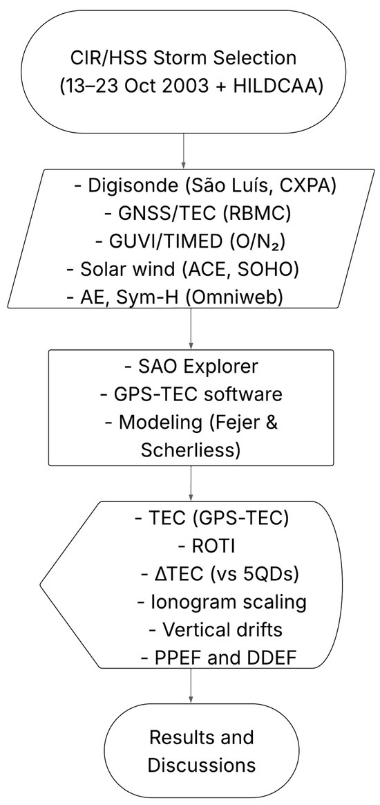
Figure 1.
Schematic diagram of the methodology used to analyze the ionospheric response to the CIR/HSS-driven geomagnetic storm. The diagram summarizes data sources, processing steps, empirical modeling, and result outputs.
2.1. Solar and Interplanetary Parameters and Geomagnetic Indices
The data for CHs and HSSs were obtained from http://www.solen.info/solar/ (accessed on 28 August 2024) and http://www.solarmonitor.org/ (accessed on 28 August 2024). Solar wind and IMF parameters were measured by the Advanced Composition Explorer (ACE) satellite, located at the Lagrange point L1 (1 AU from Earth). These data, along with geomagnetic indices such as AE and Sym-H, were retrieved from the OMNIWeb platform, accessible at https://omniweb.gsfc.nasa.gov/ (accessed on 28 August 2024).
2.2. Digisonde Measurements
The Brazilian low-latitude ionosphere was primarily investigated by analyzing ionograms obtained from Digisonde measurements [32], in the equatorial region at São Luís and around the southern crest of the EIA, at Cachoeira Paulista. F-region parameters such as the virtual height of the F-layer (), the peak height (), and the critical frequency () were derived and analyzed. The ionograms were recorded at a 15 min temporal resolution. The Digisonde data were retrieved from the EMBRACE website (http://www2.inpe.br/climaespacial/portal/en/), accessed on 30 August 2024.
Figure 2 displays the spatial distribution of the GNSS and Digisonde stations used in this study, covering a wide range of dip latitudes across the Brazilian sector. These locations are detailed in Table 1, which lists the observation methods, station codes, geographic coordinates, geomagnetic inclination, and dip latitudes. This spatial configuration allows us to examine the equatorial and low-latitude ionospheric response with latitudinal coverage extending from near the magnetic equator to the southern crest of the EIA.
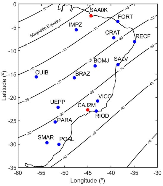
Figure 2.
Spatial distribution of the GNSS and Digisonde stations used in this study. Blue dots represent the locations of GNSS stations employed to derive TEC datasets, while red dots indicate the positions of Digisonde instruments. The black lines represent geomagnetic inclination contours, including the magnetic equator, serving as references for the EIA region.

Table 1.
Stations used for digital ionospheric sounding (Digisonde) and GNSS (GPS) measurements, including their codes, observational methods, geographical coordinates (latitude and longitude), geomagnetic inclination, and dip latitudes. The stations are organized by dip latitude and instrument type, covering the Brazilian low-latitude region from the equatorial to the southern crest zones of the EIA.
The ionospheric parameters analyzed in this work, including the virtual height of the F-layer (), the peak height of the F2-layer (), and its critical frequency (), were derived from Digisonde ionograms recorded at 15 min intervals. These measurements were obtained from São Luís (equatorial region) and Cachoeira Paulista (southern EIA crest).
No pre-processing was applied to the raw ionogram data. The scaling of the ionospheric parameters was performed manually using the SAO Explorer Software version 3.6.3 [33], available at https://ulcar.uml.edu/SAO-X/SAO-X.html (accessed on 30 August 2024). In this longitudinal sector, Universal Time (UT) is related to Local Time (LT) by the offset .
Furthermore, as a baseline, we employed the three-hour moving average of the five quietest days (5QD) in October 2003, determined based on the index. These data were obtained from http://wdc.kugi.kyoto-u.ac.jp/qddays/ (accessed on 9 September 2024). This baseline allows for the identification of periods with minimal geomagnetic disturbance, ensuring that the analyzed ionospheric behavior corresponds to quiet-time conditions.
2.3. Global Positioning Systems GPS-TEC
The TEC is defined as the total number of electrons integrated along the line of sight between a radio transmitter and a receiver. It is expressed in electrons per square meter, with one TEC unit (TECU) corresponding to electrons/m2. TEC is a fundamental parameter for monitoring and analyzing ionospheric variability over large spatial scales, offering valuable insights into phenomena such as the development of the EIA, EPBs, wave activity, and other ionospheric disturbances.
In this study, we employ a combination of ionospheric parameters and indices—specifically, TEC, TEC (TEC variation relative to the five quietest days, 5QD), and the Rate of TEC Index (ROTI)—to analyze the occurrence of plasma irregularities. ROTI is a widely adopted index for detecting ionospheric irregularities and is derived from the standard deviation of the rate of change of the Slant Total Electron Content (STEC) over a 5 min interval. This index is particularly effective for characterizing ionospheric disturbances, including EPBs.
The Rate of TEC (ROT) quantifies the temporal variation in STEC and is expressed as
where represents the time interval between consecutive STEC measurements.
To assess the degree of ionospheric irregularity, the ROTI is computed as the standard deviation of ROT over the defined 5 min interval as
Since ROTI is inherently influenced by the satellite–receiver geometry, elevation angle constraints are typically applied to mitigate multipath effects and reduce oblique propagation errors. In this study, we adopt a minimum elevation angle of 45° to ensure the reliability of STEC-derived ROTI values.
The classification of ionospheric irregularities is based on ROTI values: no irregularities (); weak irregularities (); moderate irregularities (); and strong irregularities ().
The GPS observational data used in this study were provided by the Brazilian Network for Continuous GPS Monitoring (RBMC), managed and operated by the Brazilian Institute of Geography and Statistics (Instituto Brasileiro de Geografia e Estatística, IBGE). RBMC data can be accessed directly at https://geoftp.ibge.gov.br/informacoes_sobre_posicionamento_geodesico/rbmc/ (accessed on 17 September 2024).
These data were used to compute the Vertical Total Electron Content (VTEC) using the GPS-TEC software version 2.9.5 developed by Gopi Seemala (for further details, see [34]). The VTEC was calculated by averaging the values from GPS satellites with elevation angles above 30°, within the field of view of the GPS-TEC receiver at any given time. Although Brazil currently has an extensive network of GPS receivers and significant progress has been made in space weather and aeronomic studies in recent years, the situation in 2003 was different. At that time, only a limited number of RBMC receivers were available. Therefore, our analysis is based on a restricted set of stations strategically located in the most representative ionospheric regions of Brazil: the equatorial zone, low-latitude sector, and the South Atlantic Magnetic Anomaly (SAMA) region.
2.4. Global Ultraviolet Imager (GUVI) Database
To examine the relationship between TEC variations and thermospheric composition, global changes in the [O]/[N2] ratio were obtained from the Global Ultraviolet Imager (GUVI) database, available at http://guvitimed.jhuapl.edu/ (accessed on 19 September 2024).
2.5. Fejer and Scherlies Model Description
To further understand the driving forces behind the ionospheric dynamics, the strength of the vertical drift, as well as the quiet and disturbed Pre-Reversal Enhancement (PRE), were estimated using the empirical model developed by Scherliess and Fejer [16]. This model leverages measurements of the auroral electrojet (AE) index to estimate the mean ionospheric vertical plasma drifts as a function of longitude, local time, and solar activity. It provides empirical estimates of storm-time vertical plasma drifts based on auroral electrojet activity and high-latitude convection patterns, incorporating the effects of both prompt penetration and disturbance dynamo electric fields. The model primarily captures large-scale variations and the average behavior of vertical plasma drifts, relying on statistical relationships rather than resolving high-resolution temporal or spatial details.
The time-dependent variability of vertical drift penetration during geomagnetic disturbances evolves over short timescales, depending on the behavior of penetration electric fields [16]. These variations are driven by electric field perturbations originating from the ionospheric and magnetospheric dynamo systems. Disturbed drifts are analyzed concerning the AE index, which serves as a proxy for high-latitude auroral activity and associated electric field perturbations [35], as well as the energy input into the high-latitude ionosphere [36]. This empirical framework helps quantify the relationship between high-latitude auroral activity and equatorial ionospheric drifts, contributing to a broader understanding of large-scale plasma dynamics.
3. Results and Discussions
3.1. CIR/HSS-Driven Geomagnetic Storm on 12–23 October 2003
Figure 3 shows a sequence of solar disk images captured by the Michelson Doppler Imager (MDI), part of the Solar Oscillations Investigation (SOI) aboard the SOHO (Solar and Heliospheric Observatory) spacecraft. The images, taken between 12 and 23 October 2003, are shown in the Ni I 6768 Å (visible continuum) wavelength. They highlight transequatorial CHs, visible as dark regions that co-rotate with the Sun.
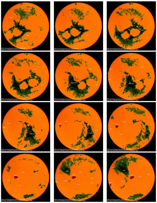
Figure 3.
SOHO images showing the coronal hole CH63 from 12 to 24 October 2003. The green areas represent the coronal hole structure as it evolves, with active regions labeled across different dates. These observations were captured in the ultraviolet emission spectrum, highlighting key coronal features.
As is well known, CHs are most geoeffective when aligned near the solar disk’s central meridian and around the solar equator, allowing for maximal interaction with Earth’s magnetosphere [8]. In the images, a large transequatorial coronal hole, designated CH63, crossed the center of the solar disk and reached the central meridian between 12 and 18 October. Subsequently, it showed a reduction in area compared to its previous solar rotation, losing much of its extent in the northern hemisphere and merging with remnants of coronal hole CH59 in the southeastern quadrant.
During this period, HSS and CIR directed toward Earth were detected by ACE onboard instruments. These interactions led to enhanced coupling with Earth’s magnetosphere, resulting in a moderate (Sym-H = −100 nT) and prolonged geomagnetic storm from 13 to 23 October, associated with a HILDCAA event, as defined by Tsurutani and Gonzalez [23].
After 17 October, as the coronal hole rotated westward and moved out of direct alignment with Earth, its geoeffectiveness gradually diminished, leading to a decrease in geomagnetic storm activity and reduced impacts on Earth’s environment.
To characterize the interplanetary and geomagnetic conditions associated with this CIR-driven storm, we utilized 1 min average datasets of the solar wind speed (Vsw), the proton density (Nsw), the Z-component of the interplanetary magnetic field (Bz), the interplanetary electric field component (Ey, mV/m), the geomagnetic symmetric disturbance index (Sym-H, an analog of the Dst index), and the auroral electrojet index (AE). These data are displayed in Figure 4.
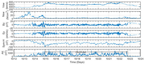
Figure 4.
Solar wind and geomagnetic conditions during the CIR-driven storm from 12 October (00:00 UT) to 24 October (00:00 UT), 2003. The figure presents the following, from top to bottom: solar wind speed (Vsw, km/s), proton density (Nsw, cm−3, the Z-component of the interplanetary magnetic field (Bz, nT), the Electric Field (Ey, mV/m), the symmetric disturbance index (Sym-H, nT), and the auroral electrojet index (AE, nT). An HILDCAA event is highlighted, beginning on 15 October 2003, and persisting until 22 October 2003.
Between 12 and 23 October 2003, HSSs were detected, evidenced by a significant growth in solar wind speed, which exceeded 400 km/s on 13 October and peaked at 800 km/s on 15 October. The corresponding peak in Nsw indicates the presence of a CIR—a compressed plasma region formed at the interface between fast and slow solar wind streams. Proton density showed substantial variability, with a major peak on 13 October exceeding 40 cm−3, signaling the arrival of the CIR [37]. The Bz component of the interplanetary magnetic field fluctuated significantly, ranging between −20 and 20 nT, particularly on 14 October during the storm’s main phase.
It is crucial to highlight that during geomagnetic storms, particularly when the interplanetary magnetic field Bz is directed southward (Bz < 0), the impacts of PPEFs and DDEFs become especially prominent. During the main phase of the storm, a PPEF event is often observed, characterized by conditions where Bz < 0 and Ey > 0 due to magnetic reconnection processes as can be observed in Figure 4. These reconnection events allow the solar wind to couple directly with Earth’s magnetosphere, resulting in the rapid penetration of high-latitude electric fields to low-latitude and equatorial regions. PPEF can quickly alter its polarity and direction, influencing both daytime and nighttime ionospheric dynamics [12,16,38].
The Sym-H index reached a minimum of −100 nT, indicating a moderate geomagnetic storm. Sym-H measures the ring current intensity, which correlates with the energy stored in the magnetosphere during geomagnetic storms [1]. The storm’s prolonged recovery phase was driven by sustained energy input, resulting from multiple magnetic reconnection events triggered by large fluctuations in Bz. These fluctuations were associated with Alfvén waves embedded in the high-speed solar wind streams. Magnetic reconnection occurs when the IMF is oriented southward for extended periods, enabling direct coupling with Earth’s geomagnetic field [1,8]. An intense southward IMF can lead to enhanced plasma sheet convection, strengthening the ring current and intensifying the geomagnetic storm.
The AE index, which tracks auroral activity, increased sharply on 14 October, marking a beginning of significant geomagnetic disturbances. An HILDCAA event was recorded from 15 to 22 October, indicating continuous, long-lasting auroral disturbances during this period. This persistent activity reflects the sustained impact of the HSS and CIR on Earth’s magnetosphere, contributing to prolonged geomagnetic storm conditions.
According to the first empirical criteria, a High-Intensity Long-Duration Continuous AE Activity (HILDCAA) event must satisfy four conditions: (i) the AE index must reach or exceed 1000 nT; (ii) the AE index should not drop below 200 nT for more than two continuous hours; (iii) the event must last for at least two days; and (iv) it should occur outside the main phase of a geomagnetic storm, specifically during its recovery phase [23].
In addition to the traditional criteria, complementary parameters have been suggested for identifying HILDCAA events, including moderate fluctuations in the Sym-H index (remaining ≥ −100 nT), the presence of high-speed solar wind streams, and high-frequency oscillations of the IMF Bz around zero, with amplitudes of approximately ±10 nT [39]. Under these stricter conditions, approximately ten HILDCAA events were recorded during the highly active year of 2003. However, a slight relaxation of these criteria increases the number of identified HILDCAA events to twenty-six [40], thereby enhancing the statistical basis for ionospheric studies.
As illustrated in Figure 4, all of these conditions were met from 15 to 22 October 2003. The AE index exceeds 1000 nT and remains predominantly above 200 nT for the remainder of the interval, with only brief drops. The elevated AE levels persist for approximately nine days, fulfilling the minimum duration requirement. Moreover, the Sym-H index indicates that the main phase of the geomagnetic storm ended on 14 October, confirming that the HILDCAA occurred during the subsequent recovery phase. In addition to satisfying the traditional criteria, this event also aligns with the complementary parameters proposed in more recent studies, including sustained high-speed solar wind streams, moderate Sym-H fluctuations (remaining above −100 nT), and IMF Bz oscillations of approximately ±10 nT. These observations collectively support the classification of this interval as an HILDCAA event [23,39,40].
3.2. F-Layer Heights and Plasma Frequencies
Figure 5 presents a series of time-series plots from 12 to 23 October 2003, highlighting key ionospheric parameters derived from Digisonde measurements at the São Luís (SAA0K) station, located in the equatorial region. The top panel illustrates the Sym-H index, referencing geomagnetic activity during this period.
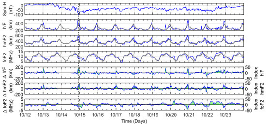
Figure 5.
Temporal evolution of the Sym-H index and ionospheric parameters (, , and ), along with their respective deviations, during the moderate geomagnetic storm of 12–23 October 2003, for the equatorial region (São Luís). The 5QD average variations of , , and are represented by the black line, with the standard deviation shaded in light gray. The green lines indicate the calculated indices of , , and , showing deviations in percentile form relative to quiet conditions. The dashed line corresponds to the onset of the HILDCAA event, marking the recovery phase of the geomagnetic storm.
The subsequent panels display ionospheric parameters, including F-layer heights, and (in km), and the plasma critical frequency, (in MHz). During the storm’s main phase on 14 October, the ionospheric F-layer experienced a significant uplift (120 km above the average 5QD) around sunset at 22:21 UT (19:21 LT). The plasma critical frequency, , which reflects the electron density in the F2-layer (), decreased compared to the 5QD baseline during the storm’s main phase, likely due to plasma depletion caused by the F-layer uplift and removal of plasma from lower heights.
For completeness, the lower panels display the deviations of these parameters (, , and ) from their quiet-day baselines. During the storm’s main phase (13–15 October), positive deviations of approximately 120 km were observed in both and , indicating storm-induced uplift. Conversely, exhibited a negative deviation of around 3 MHz, reflecting a reduction in plasma densities. The recovery phase of the storm extended from 22:21 UT (19:21 LT) on 14 October to 23:59 UT on 23 October, lasting approximately 9 days [41].
Throughout this period, fluctuations in and were observed, particularly when the Auroral Electrojet (AE) index showed intense variations (∼1000 nT amplitudes) and when the Sym-H index exhibited slight decreases (<−50 nT).
Additionally, an amplification of the drift was evident around 23:00 UT (20:00 LT) from 15 to 23 October, with the most pronounced effect observed on 20 October. On this day, a significant uplift of the F-layer height (∼150 km) was recorded, accompanied by a plasma density decrease () of approximately 5 MHz. A similar pattern was observed at 23:00 UT (20:00 LT) on 22 October. Throughout the rest of the period (14 to 23 October), F-layer height variations remained within ∼100 km, while exhibited a decrease of no more than 2 MHz, except on 22 October, when a notable reduction in F-layer height (∼100 km) and plasma density (∼3 MHz) was observed at 23:00 UT (20:00 LT).
These long-lasting perturbations are likely associated with DDEF, as they persist well into the recovery phase, even after the IMF Bz and Ey have returned to quiet levels. Unlike PPEF, which act on shorter timescales (minutes to hours) and are directly linked to IMF fluctuations, DDEF arises from storm-induced changes in global thermospheric circulation and resultant electric fields [42,43,44]. These changes are driven by Joule heating and ion drag at high latitudes, which modify the neutral wind system and generate electric fields that propagate equatorward [43,44]. The effects of DDEF are typically observed on longer timescales (several hours to days) and are more prominent during nighttime, due to enhanced wind-driven dynamo processes in the ionosphere [42,44].
Additionally, the indices , , and were calculated using deviations from the standard deviation of the 5 Quiet Days (5QD), normalized by local mean values during nighttime (0 to 3 LT); see [45] for more details. These indices display similar behavior to the deviations but are expressed in percentile form, providing a clearer quantification of the extent of ionospheric increase or decrease relative to baseline conditions in response to geomagnetic activity.
The F-layer heights show significant uplifts around the time of PRE occurrence during the storm’s main phase and for several days into the recovery phase. Under quiet conditions, the PRE is associated with an increase in the eastward electric field in the ionospheric E-region, resulting from the strong conductivity gradient across the day–night terminator during post-sunset hours [46]. However, under magnetospheric and auroral substorm disturbances, high-latitude dawn–dusk electric fields can rapidly penetrate the equatorial region due to under-shielding conditions in the Region-2 (R2) current system. The balance between Region-1 (R1) and R2 field-aligned currents (FACs), along with their associated horizontal closure currents, plays an important role in this process. These currents are strongly influenced by solar wind parameters, including speed, density, temperature, and magnetic field strength [2,47].
The polarity of the PPEF shows a dependence on local time [17], resembling the quiet-time ionospheric dynamo electric field, as demonstrated in model simulations [48]. The PPEF maps along the highly conductive geomagnetic field lines to the equator, reinforcing the background eastward electric field and enhancing the vertical plasma drift—a phenomenon widely discussed by several authors [49,50].
The disturbed-time PRE can have at least two important implications: the recurrence of the EIA during nighttime, typically around 16 LT, and the triggering of plasma irregularities in the equatorial region, which will be discussed in more detail later. Furthermore, PPEF electric fields can penetrate during different phases of a magnetic storm due to sudden changes in the polarity of the IMF Bz, thereby adding complexity to ionospheric electrodynamics [10,38,51].
As shown in Figure 5, the and increased by nearly 50% above the 5QD average, while the exhibited only a modest decrease compared to the quiet-day baseline, with a deviation of approximately 25% during the storm’s main phase at 22:21 UT (19:21 LT). The sudden uplift of the F-region during the storm’s main phase, driven by PPEF and occurring around the time of the PRE, may have created favorable conditions for the development and intensification of plasma irregularities. Although EPBs are commonly observed during the equinoctial period from October to March in this longitudinal sector, the enhanced vertical drift likely displaced plasma to higher apex altitudes over the magnetic equator, favoring the upward development of irregularities and their extension to latitudes beyond the EIA crests. Spread-F signatures were observed in the equatorial ionograms recorded at São Luís throughout the entire interval, extending into the late recovery phase. To assess the occurrence of EPBs, we use GPS-TEC data and its derived index, ROTI. This topic is further discussed in the next section.
Figure 6 presents the F-layer parameters extracted from Digisonde measurements around the southern EIA crest, at Cachoeira Paulista. Similar to the equatorial region, multiple F-layer uplifts are evident in from the beginning of the storm to the end of the recovery phase. Simultaneous uplifts over the equator and at the southern EIA crest highlight the action of the under-shielding eastward PPEF, particularly during deeper incursions of IMF Bz southward and decreases in the Sym-H index. PPEF enhances the fountain effect by strengthening the vertical plasma drift, causing the expansion of the southern crest of the EIA to higher latitudes [20,52]. Additionally, PPEF can penetrate the ionosphere at different stages of a magnetic storm due to sudden shifts in the polarity of the IMF Bz, altering ionospheric electrodynamics [53].
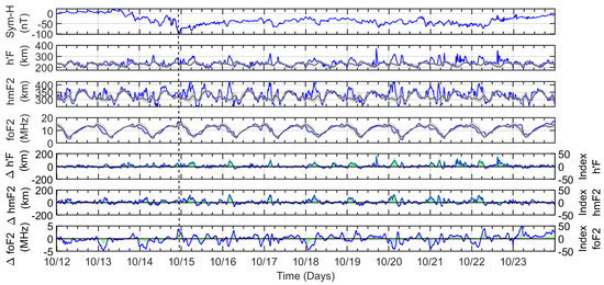
Figure 6.
Temporal evolution of the Sym-H index and ionospheric parameters (, , and ), along with their respective deviations, during the moderate geomagnetic storm of 12–23 October 2003, for the EIA crest region (Cachoeira Paulista). The 5QD average values of , , and are represented by black lines, with the standard deviation shaded in light gray. The green lines indicate the calculated values of , , and , showing deviations in percentile form relative to quiet conditions. The dashed line marks the onset of the HILDCAA event, indicating the beginning of the storm’s recovery phase.
As mentioned above, PPEF arises due to an imbalance between the high-latitude R1 and R2 current systems, typically near the beginning of geomagnetic disturbances, when large variations in the IMF Bz take place [47]. These electric fields penetrate promptly from high to low latitudes, leading to rapid changes in the vertical plasma drift [9]. Although PPEFs generally last for only a few minutes to hours before the current systems reach equilibrium, their impact on the equatorial ionosphere can be significant, as they enhance the vertical drift and contribute to the EIA intensification [12,15,16]. Previous studies have demonstrated that PPEFs are crucial in driving short-term ionospheric disturbances, particularly during the main phase of storms, when IMF fluctuations are more pronounced [13,14].
In fact, spread-F structures were consistently observed in equatorial ionograms recorded in São Luís throughout the entire interval, persisting until the end of the recovery phase. This indicates that ionospheric irregularities remained active for an extended period, likely influenced by ongoing perturbations in the electrodynamic processes controlling plasma stability. However, the interpretation of F-layer uplifts in and in the third and fourth panels must be approached with caution due to the presence of spread-F. Spread-F is caused by post-sunset plasma instabilities, often associated with the development of EPBs [19]. The occurrence of spread-F can introduce significant uncertainties in the estimation of ionospheric parameters, as it leads to distorted ionograms and unreliable echo traces [21,54]. Consequently, data processing algorithms may struggle to provide accurate and values under such conditions.
These limitations will be further discussed in Section 3.7, where the impact of spread-F on Digisonde measurements is examined in more detail. To complement the Digisonde observations and assess the development of ionospheric irregularities, we employ GPS-derived TEC and its associated ROTI.
Finally, it is worth noting that the prolonged recovery phase of this storm was characterized by an HILDCAA event. This study highlights not only the sustained effects of a moderate geomagnetic storm but also underscores the significant influence of HILDCAA events on the equatorial and low-latitude ionosphere, driven by persistent high-speed solar wind streams interacting with Earth’s magnetosphere.
3.3. Plasma Drift: Fejer–Scherliess Model
Understanding the variations in equatorial vertical plasma drifts during geomagnetic disturbances is essential for assessing their impact on the low-latitude ionosphere. To achieve this, we employ the empirical model developed by Scherliess and Fejer [16], which estimates storm-time equatorial plasma drifts based on AE activity. This model enables us to quantify the contributions of PPEF and DDEF to vertical drift perturbations, providing information on how geomagnetic storms, particularly CIR/HSS-driven events, influence equatorial electrodynamics. By comparing the modeled storm-time vertical drifts with observations from Digisonde data, we assess the role of PPEF in driving F-layer uplifts, plasma density depletions, and the expansion of the EIA. Additionally, we investigate the longer-term influence of DDEF during the extended recovery phase.
Figure 7 presents, from top to bottom, the following: the vertical component of the vertical component of IMF Bz and the Sym-H index, both expressed in nT. From the third panel downward, the following parameters are shown: the calculated mean (quiet-time) vertical drift, (Vmean); the disturbed vertical drift, (Vd storm); the total vertical drift, (Vd total); and the PPEF-driven and DDEF-driven vertical drift components, labeled as PPEF and DDEF, respectively, all expressed in m/s. The mean vertical drift velocity (Vd mean) during quiet conditions exhibits the typical diurnal pattern, with an upward drift during the day and a downward drift at night.
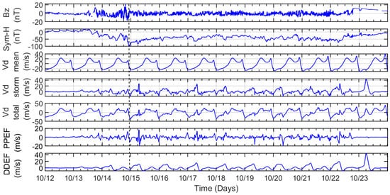
Figure 7.
Variations of the interplanetary magnetic field (Bz) in nT, the Symmetric Disturbance Index (Sym-H) in nT, and empirical calculations of the mean vertical drift (-mean), storm-time drift (-storm), total drift -total, and the PPEF- and DDEF-driven components, all expressed in m/s.
During the main phase of the storm on 14 October, the calculated disturbed vertical drift velocity (Vd total) reached approximately 10 m/s around 23:00 UT (20:00 LT), coinciding with the PRE occurrence time. This result is consistent with observations of at São Luís, as shown in Figure 5, where the F-layer height suddenly increased by about 120 km relative to the 5QD . In turn, the reduced plasma frequency, , indicates a depletion of plasma from the bottomside of the F-layer. This sudden uplift was therefore driven by the action of PPEF drift, estimated at approximately 15 m/s. Sudden F-region uplifts are often associated with rapid ionospheric plasma movements triggered by PPEF [55].
Zonal electric fields drive F-region vertical plasma drifts, particularly during the post-sunset and pre-sunrise periods when the sharp conductivity gradient and thermospheric winds in the E-region are dominant [56]. The vertical drifts are influenced by PPEF originating from magnetospheric sources and by the long-lasting DDEF associated with disturbances in neutral winds and storm-induced changes in ionospheric conductivity [48,57]. Westward perturbations attributed to electric fields penetrating from the inner magnetosphere into the equatorial region may explain the occurrence of disturbed downward drifts, whereas upward drifts are often linked to the generation of equatorial spread-F [12].
The nocturnal enhancement of the equatorial F-layer is primarily attributed to the intensification of the eastward electric field, which is influenced by thermospheric winds through the F-region dynamo [58,59]. Additionally, the prereversal enhancement in upward drift velocity around sunset creates favorable conditions for the onset of equatorial spread F, plasma bubbles, and scintillations [60]. The PRE is commonly observed during solar maximum years; however, it tends to be significantly diminished or completely absent during solar minimum periods [48].
3.4. TEC Variations
To investigate the ionospheric response to the CIR/HSS-driven geomagnetic storm, we analyze TEC data from all available Brazilian stations, focusing on three ionospherically representative regions: the magnetic equator, the southern crest of the EIA, and the SAMA. Figure 8 presents, from top to bottom, the TEC variations (blue line) alongside the average of the 5QDs (black line) for stations located near these regions.
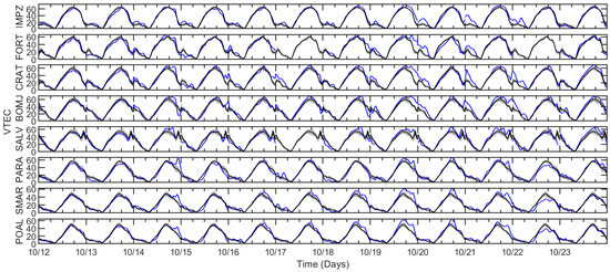
Figure 8.
Variation of VTEC during the CIR-driven geomagnetic storm of 12–23 October 2003, spanning from the equatorial region to southern crest zones of the EIA. The blue and black lines represent the storm-time VTEC values and the five quietest days (5QD) baseline, respectively.
Figure 9 shows the latitudinal variation of VTEC relative to the 5QD average (black line), along with the corresponding percentile deviations (VTEC) and the VTEC Index (green), which represents VTEC normalized to the mean nighttime value from 00–03 LT.
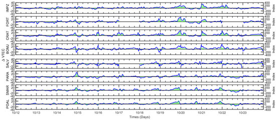
Figure 9.
Variation of VTEC during the CIR-driven geomagnetic storm of 12–23 October 2003, for dip latitudes ranging from the equatorial region to the southern crest zones of the EIA.
Throughout the interval, VTEC shows mostly positive deviations compared to the quiet-day baseline, with the most pronounced intensification occurring during the main phase of the storm on 14 October, particularly over the southern crest of the EIA at PARA. The VTEC enhancement on this day coincides with the strongest eastward PPEF, which likely intensified the vertical drift, thereby enhancing the fountain effect and redistributing ionization toward higher latitudes. During the latter part of the recovery phase, on 19–21 October, notable VTEC increases were observed across a broad latitudinal range, extending from the equatorial region to the SAMA, particularly in the afternoon (∼18 UT or 15 LT) and post-midnight hours (∼03 UT or 01 LT). These enhancements suggest the sustained influence of DDEF, which persisted well into the storm’s recovery phase. Additionally, VTEC intensifications were recorded following southward excursions of the IMF Bz and decreases in the Sym-H index, indicating episodes of storm-driven electrodynamic modifications affecting the low-latitude ionosphere.
The VTEC enhancement observed on 14 October at stations near the SAMA (e.g., POAL and SMAR) suggests a poleward expansion of the EIA, a phenomenon typically associated with intensified vertical drifts during geomagnetic disturbances. From 19 to 22 October, a second phase of intensified VTEC variations was observed, extending from IMPZ (equatorial region) to POAL (SAMA region). This latitudinal shift suggests that disturbed electric fields, including long-lasting DDEF and possible episodes of daytime PPEF, played a role in modifying ionospheric plasma transport. The SAMA region exhibited significant VTEC increases throughout the storm, highlighting its heightened susceptibility to geomagnetic disturbances due to its weaker geomagnetic shielding. The presence of enhanced VTEC in this region supports the idea that storm-time electric fields can exert a more pronounced influence over areas with reduced magnetic field intensity, further affecting plasma redistribution dynamics.
The PRE represents an intensification of the vertical drift around dusk, driven by interactions between neutral winds and zonal electric fields near the day–night terminator. This feature is highly sensitive to geomagnetic disturbances and plays an important role in storm-time ionospheric restructuring [56]. The post-sunset VTEC enhancements were observed on 18–21 October, extending from the equatorial region to SAMA during the evening hours. These enhancements suggest that storm-induced PPEF may have reinforced the PRE, thus intensifying upward plasma drifts. Such interactions between PPEF and the PRE could have played a role in sustaining the storm-time EIA structure well into the nighttime hours.
The sustained VTEC enhancement observed until 21 October coincided with solar wind speeds exceeding 600 km/s, further demonstrating the prolonged effects of the CIR/HSS-driven storm. Unlike the rapid recovery typical of CME-driven storms, CIR-driven storms introduce recurrent episodes of disturbed electrodynamics, leading to longer-lasting positive storm phases in TEC. These findings are consistent with previous results of [61] that emphasize the extended nature of ionospheric disturbances associated with CIR/HSS.
On 22 October 2003, the ionospheric response exhibited a transition from the persistent VTEC enhancements observed in the preceding days. While VTEC remained elevated across all analyzed regions during the main and recovery phases, on this day, the increase diminished significantly, and in the vicinity of the SAMA, VTEC values dropped below quiet-time levels. This behavior coincided with a notable reduction in geomagnetic activity, as the Sym-H index, which had fluctuated around −50 nT, returned to approximately 0 nT, indicating the dissipation of storm-induced perturbations in the ring current. Simultaneously, the solar wind speed, which had previously remained elevated at around 800 km/s, decreased to nearly 400 km/s, suggesting a weakening of the high-speed stream influence. The IMF and the dawn–dusk electric field, , exhibited no significant oscillations, indicating that PPEF and DDEF—previous drivers of ionospheric disturbances—were no longer active.
In the absence of these electric fields, the dominant mechanisms governing ionospheric plasma transport and density distribution transitioned toward recombination processes and neutral composition effects. The weakening of vertical plasma transport, combined with enhanced recombination at lower altitudes, contributed to the observed TEC depletion. Additionally, changes in thermospheric composition—particularly a reduction in the oxygen-to-nitrogen ratio (O/N2)—likely played a role in decreasing plasma production efficiency. The suppression of the PRE further inhibited post-sunset plasma uplift, leading to a weakened EIA and a reduction in ionospheric electron content.
These findings suggest that the transition from a disturbed to a quiet ionosphere during CIR/HSS-driven storms involves not only the cessation of storm-time electric fields but also thermospheric adjustments and chemical recombination effects. These processes can lead to delayed negative storm phases, particularly in regions such as the SAMA, where weaker magnetic shielding facilitates enhanced recombination and plasma loss.
Moreover, the latitudinal VTEC variation on 18–21 October highlights a well-developed EIA, extending throughout the interval due to the continuous strengthening of disturbed electric fields, which drive the EIA to higher latitudes near the SAMA region (POAL, dip: −20°). During the storm’s recovery phase, embedded within a HILDCAA event, TEC intensifications are observed, particularly during mild southward Bz excursions. This suggests possible episodes of daytime PPEFs and enhancements around the PRE, likely inducing enhanced vertical drifts and positive ionospheric storms across a wide area.
Although the EIA is typically prominent in equinoctial months like October, this event indicates a storm-time EIA that persisted into the nighttime hours. While the moderate CIR-driven storm did not appear to produce a Super Fountain effect [20], it sustained a significant EIA presence at the boundary between the EIA crest and the SAMA.
3.5. Changes in Thermospheric Composition
In Section 3.3 and Section 3.4, we analyzed the ionospheric response to storm-induced electric fields, including variations in vertical plasma drifts and TEC intensifications over low-latitude regions. However, the prolonged TEC enhancements observed from 14 to 21 October, followed by a distinct depletion phase on 22 October, suggest the influence of additional factors beyond electrodynamic forcing. This section examines the contribution of neutral composition changes, specifically variations in the oxygen-to-nitrogen ratio ([O]/[N2]), to the observed ionospheric behavior. Using measurements from the GUVI instrument, we assess the spatial and temporal evolution of thermospheric composition over Brazil, highlighting its role in sustaining positive ionospheric storm phases and in subsequently driving TEC depletions during the later recovery stage.
Figure 10 presents global maps showing variations in the [O]/[N2] ratio for a geomagnetically quiet day (12 October) and for subsequent disturbed days, with satellite passes over Brazil. The horizontal scale indicates both UT and LT, while the color bar on the right side of the map denotes regions with high [O]/[N2] ratios (red) and low [O]/[N2] ratios (black). Vertical white bands indicate potential detector contamination caused by energetic particles, which also resulted in increased noise, as described in [62].
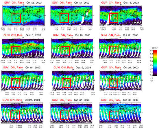
Figure 10.
Global maps of the [O]/[N2] ratio obtained from the GUVI experiment onboard the TIMED satellite for a geomagnetically quiet day (12 October) and disturbed days (13–23 October). The red rectangle highlights the South American region, where Brazil is located.
Enhanced [O]/[N2] ratios were observed over Brazil near the southern crest of the EIA (in red) from 14 to 20 October, suggesting that changes in neutral composition contributed to the increased plasma density/TEC observed over Brazil. This phenomenon can be explained as follows: geomagnetic storms increase particle precipitation and Joule heating, driving equatorward meridional winds in the thermosphere and altering zonal wind patterns. These shifts, partially governed by the Coriolis effect [63], transport oxygen-depleted air with modified [O]/[N2] ratios from high to mid and low latitudes across various longitudes. This redistribution of atmospheric composition plays a critical role in ionospheric dynamics during geomagnetically disturbed periods.
A positive ionospheric storm results from thermospheric composition changes triggered by geomagnetic activity at auroral latitudes, leading to a reduction in molecular nitrogen (N2) and an increase in atomic oxygen (O). Under quiet ionospheric conditions, the [O]/[N2] ratio typically remains stable (indicated by green areas), with values generally ranging between 0.6 and 0.7, reflecting a balanced thermospheric environment with minimal geomagnetic forcing [64].
During geomagnetic storms, increased solar energy input at auroral latitudes enhances ionization and alters thermospheric composition [3,49,65]. Rather than directly converting oxygen ions to nitrogen ions, the enhanced ionization and heating raise the neutral density of nitrogen molecules, leading to a relative decrease in atomic oxygen concentration. This change lowers the [O]/[N2] ratio, which can drop to as low as 0.1 or below during intense geomagnetic storms. This reduction is primarily due to shifts in thermospheric circulation that redistribute neutral constituents, rather than a direct chemical conversion between O and N2 ions [49].
Significant increases in the [O]/[N2] ratio in the F region during the large geomagnetic storm on 24 November 1982, were reported [66]. In this sense, our findings are consistent with those of [66], showing notable enhancements in the [O]/[N2] ratio during the recovery phase from 14 to 22 October 2003. This increase was primarily driven by a decrease in [N2], linked to the downward movement of atmospheric regions just equatorward of areas with increased [N2]. Both atmospheric upwelling and downwelling contribute to fluctuations in [O] and [N2].
Transport of atomic oxygen [O] from mid and high latitudes toward low and mid latitudes has been observed during disturbed periods, with this redistribution being more pronounced in the lower F region than in the upper F region [67,68]. The transport of lighter species, such as atomic oxygen (O), through global thermospheric wind circulation significantly influences [O] and [N2] concentrations during geomagnetic storms [49].
3.6. EIA Development
To provide a comprehensive view of the EIA response during the CIR/HSS-driven storm, Figure 11 presents a time sequence of TEC latitudinal variations from 12 to 23 October. The EIA is observed throughout this period, forming around 19:00 UT (16:00 LT) as an intensified TEC region. On quiet days, such as 12 October, the EIA maintains a well-defined structure, with the southern crest reaching no higher than 60 TECU and centered at a mean geomagnetic latitude of ∼−15°, consistent with equinox conditions [69].
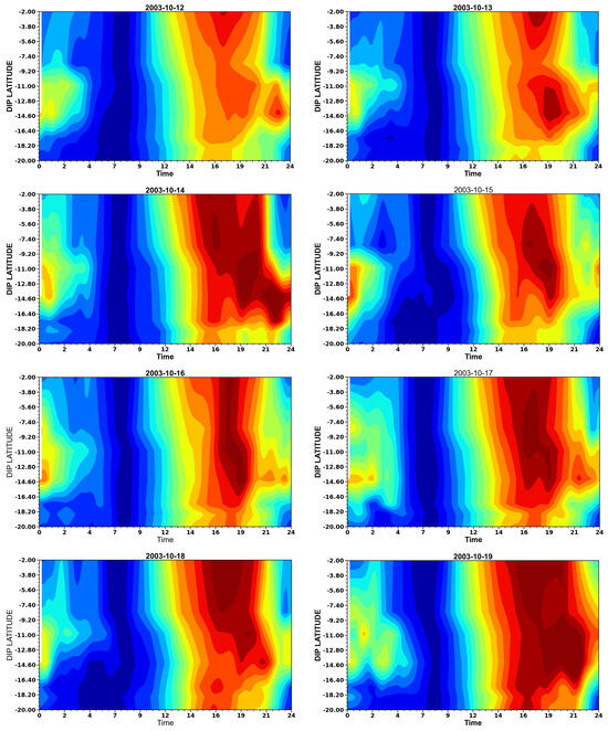
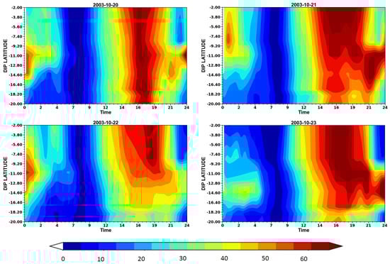
Figure 11.
Daily temporal GPS-TEC average contour plots for 12–23 October 2003.
During the storm’s main phase on 13 October, a significant intensification of the EIA is observed, with two distinct TEC peaks near the equator and at low latitudes. Notably, TEC levels remain elevated at higher latitudes past midnight, suggesting an extended fountain effect driven by PPEF [70,71]. As Sym-H reached −100 nT on 14 October, the EIA expanded poleward, with the southern crest extending beyond its typical latitudinal range [11,26,72]. The persistence of elevated TEC levels throughout the recovery phase (15–21 October) indicates the sustained influence of DDEF, which prolonged ionospheric uplift by modifying neutral wind circulation [9,48,71].
TEC remained elevated across all latitudes throughout the recovery phase, extending up to the SAMA region. The most prominent TEC intensifications occurred between 17 and 21 October, with peak values exceeding 65 TECU and persisting into the nighttime hours. These enhancements coincided with periods of strong auroral activity (AE ∼1000 nT) and sustained high solar wind speeds, indicating prolonged electrodynamic forcing in shaping the EIA evolution [63]. By 22 October, TEC values over the SAMA region dropped below quiet-time levels, marking the transition to a negative ionospheric storm, likely driven by recombination and thermospheric cooling [66].
Unlike the rapid decay observed in CME-driven storms, the prolonged TEC variations in this event highlight the characteristic effects of CIR/HSS-driven geomagnetic storms, where sustained auroral activity and long-duration magnetospheric energy input influence the low-latitude ionosphere for several days. The observed EIA expansion reached an approximately −20° dip latitude, reinforcing the role of storm-driven electrodynamics in ionospheric uplift, though without fully developing into a Super Fountain effect [20].
The EIA evolution can be attributed to the combined effects of PPEF during the main phase and DDEF-driven neutral wind circulations during the recovery phase, as indicated by [O]/[N2] variations in Figure 10.
3.7. Ionospheric Irregularities
In this section, we examine the occurrence and evolution of plasma irregularities from the equator to higher latitudes using the GPS-TEC-derived index ROTI. Spread-F traces were consistently observed in ionograms recorded by Digisondes at the equatorial region (São Luís) and the southern crest of the EIA (Cachoeira Paulista).
Figure 12 shows the temporal evolution of ionospheric irregularities, as characterized by the ROTI, across Brazilian GNSS stations spanning from the equatorial (IMPZ) to low-latitude (POAL) regions during 12–23 October 2003. October is well known for its high occurrence of ionospheric irregularities in the Brazilian sector due to the seasonal dependence of plasma instabilities, which are strongly influenced by the interplay between the PRE and background ionospheric conditions [73].
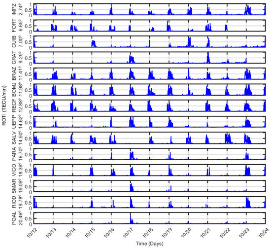
Figure 12.
Temporal variation of the Rate of TEC Index (ROTI) from 12 to 24 October 2003, across multiple stations in Brazil, arranged by dip latitude from the equatorial region to the SAMA. Each panel displays ROTI values for a given station, with blue lines indicating the occurrence and intensity of ionospheric irregularities throughout the period.
In Figure 12, moderate irregularities were first detected at 21:00 UT (18:00 LT) and persisted until 03:00 UT (00:00 LT) over Brazil’s equatorial regions and low latitudes, observed on both quiet and disturbed days. These irregularities extended up to approximately 20° S dip latitude, with notably stronger amplitudes at lower latitudes—particularly between 10° and 15° dip latitude—where plasma density gradients are typically more pronounced. By 23:00 UT (20:00 LT), ROTI values increased, indicating a poleward expansion of the irregularities. Subsequently, their amplitude decreased over the equator, though some irregularities persisted near the southern crest of the EIA.
The strongest ionospheric irregularities are observed at equatorial stations (IMPZ and FORT) and at stations located between 10° and 15° dip latitude (BRAZ, BOMJ, RECF, UEPP, and SALV). Notably, during the nighttime periods of 14–15, 17–18, 18–19, and 22–23 October, moderate irregularities extended as far as RIOD and POAL, reaching the southern crest of the EIA. These fluctuations indicate enhanced plasma turbulence and the presence of EPBs, which persisted throughout the entire recovery phase. After 18–19 October, irregularities remained present but with reduced intensity compared to the regions between 10° and 15° dip latitude, except on 23 October.
In contrast, POAL, located at −25° dip latitude, exhibits significantly weaker ROTI values, with only moderate enhancements around 16–17 October. This suggests that storm-driven disturbances had a limited impact at these latitudes, likely due to weaker PPEFs and the dissipation of equatorial irregularities before they could reach mid-latitudes. The ROTI peaks observed in the equatorial and low-latitude regions during 14–23 October align with the expected effects of storm-induced PPEFs and DDEFs, which are known to modify ionospheric electrodynamics and enhance plasma instabilities. After 23 October, ROTI values decrease significantly, indicating the dissipation of storm-induced irregularities and a gradual return to quiet ionospheric conditions.
Global maps indicate that South America, particularly Brazil, is highly susceptible to ionospheric irregularities, especially near the EIA crests during evening hours [74]. Ionospheric plasma bubbles and significant GPS phase fluctuations are most frequently observed between 20:00 and 01:00 local time, with peak activity occurring from October to March [75]. Furthermore, the highest ROTI values correspond to regions of maximum TEC gradients, which are most prominent where TEC is intensified, such as near the EIA crests [30]. Even minor storms during solar minimum can significantly influence ionospheric conditions through PPEF generated by magnetic reconnection, affecting TEC levels, intensifying plasma density gradients, and modulating the development of the EIA and EPBs [30,31].
3.8. CIR/HSS-Driven Storm and HILDCAA vs. Hallowen Storm in October 2003
The year 2003 was one of the most geomagnetically active periods in recent space-age history, marked by intense solar activity and significant space weather events. Numerous solar flares, CMEs, and CIRs triggered a wide range of geomagnetic storms, substantially impacting Earth’s magnetosphere, thermosphere, and ionosphere, as well as critical space- and ground-based technological systems. The most intense geomagnetic storm of that year occurred on 29–30 October, driven by a series of solar flares and CMEs. This storm, characterized by a Sym-H index reaching −400 nT and AE index values up to 3600 nT, generated extreme perturbations in the low-latitude ionosphere over Brazil. Notably, the storm caused an unusual strengthening of the vertical drift, with speeds around 700 m/s [71], facilitated by strong eastward PPEF.
This intense uplift led to an exceptional expansion of the EIA to latitudes well beyond the usual 20° S dip, indicative of a “Super Fountain Effect” [12,13,20,71]. EPBs have been observed extending to approximately 33° S magnetic latitude over the South American sector, reaching apex altitudes of around 2500 km above the equator [13]. Furthermore, instances of early morning development of the EIA have also been reported [12]. Despite these substantial disturbances, the ionosphere returned to quiet conditions within a few days in early November.
In this study, we analyzed ionospheric conditions in the weeks preceding the Halloween storm, focusing on the period from 13 to 20 October, when an intense CIR/HSS-driven storm occurred, associated with a large transequatorial CH on the Sun. Although this storm was less intense than the Halloween event, it generated prolonged and impactful ionospheric disturbances over the Brazilian longitudinal sector, particularly in the low-latitude region, where persistent electrodynamic processes influenced the EIA and equatorial EPBs. Continuous energy injection into the auroral region sustained geomagnetic disturbances for approximately nine days, resulting in cumulative effects such as periodic ionospheric uplifts, plasma irregularities, and persistent TEC enhancements.
Storm-time PPEFs intensified the equatorial vertical drift, triggering a pronounced fountain effect that expanded the EIA to latitudes near the SAMA region. It is well established that simultaneous TEC enhancements and plasma irregularities after sunset create favorable conditions for intense plasma gradients near the EIA crest, leading to strong ionospheric scintillations. This interplay of factors, along with thermospheric changes induced by auroral heating, sustains complex and prolonged electrodynamic processes, posing risks to technological systems, particularly those reliant on navigation and positioning accuracy.
4. Final Remarks
This study investigated the response of the Brazilian equatorial and low-latitude ionosphere to a CIR/HSS-driven geomagnetic storm that occurred from 13 to 23 October 2003, focusing on its prolonged recovery phase and associated HILDCAA event. Our findings are summarized as follows:
- The CIR/HSS-driven storm induced significant ionospheric disturbances, including an intensified vertical drift (exceeding 10 m/s), a poleward expansion of the EIA (up to −20° dip latitude), and prolonged TEC enhancements (up to 65 TECU) that persisted throughout the ∼9-day recovery phase. These effects coincided with the HILDCAA event (15–22 October), highlighting the sustained impact of CIR-driven storms on ionospheric electrodynamics.
- The storm’s main phase produced a pronounced F-layer uplift due to PPEF, with increasing by approximately 120 km at São Luís. This uplift extended the EIA crest poleward beyond its climatological range. Although the moderate CIR-driven storm did not trigger a Super Fountain Effect, it resulted in a sustained positive ionospheric storm, with TEC values remaining 30–50% higher than quiet-time levels across low-latitude and SAMA regions.
- Thermospheric composition changes, as indicated by variations in the [O]/[N2] ratio, played an important role in ionospheric density fluctuations. Enhancements in [O]/[N2] (exceeding 50%) coincided with TEC increases, while reductions in this ratio were associated with plasma depletion—particularly near the SAMA—underscoring the combined roles of electrodynamic forcing and neutral dynamics in storm-time ionospheric behavior.
- Periodic fluctuations in F-layer heights were observed throughout the recovery phase, particularly from 16 to 22 October, with deviations in , , and reaching ±100 km, ±100 km, and ±4 MHz, respectively. Negative excursions in and were mainly seen over the equator, while only positive uplifts were recorded at the southern EIA crest. This spatial pattern suggests the influence of DDEF and related neutral wind circulations, which drive equatorward winds and induce downward plasma drifts near the magnetic equator while sustaining uplift at low latitudes due to meridional wind surges and recombination suppression [52].
- TEC analysis revealed an extended fountain effect, with the EIA reaching up to −20° dip latitude and persisting for several days. Unlike transient positive storm phases typically observed in CME-driven storms, CIR/HSS-driven storms support sustained plasma redistribution. TEC variability during post-sunset hours suggests that storm-induced PPEF may have interacted with the PRE, further enhancing upward drifts and maintaining the EIA structure.
- Plasma irregularities detected via ROTI expanded poleward, particularly between 10° and 15° dip latitude, with values ranging between 0.5 and 1 TECU/min. This indicates an increased likelihood of ionospheric scintillations and degraded GNSS performance within these regions.
In conclusion, our findings emphasize the relevance of systematic investigations of CIR/HSS-driven storms, which, though moderate in intensity, are typically long-lasting and frequently associated with HILDCAA events. These storms drive a broad spectrum of space weather effects that influence the Earth’s ionosphere and technological systems. While they may not cause immediate disruptions, their cumulative effects can degrade the performance of systems reliant on GNSS and satellite-based communications.
Author Contributions
Conceptualization, V.K. and C.M.N.C.; methodology, S.A., V.K. and C.M.N.C.; software, V.G.P.; validation, J.A.d.E.S.T. and L.L.T.; formal analysis, S.A.; investigation, S.A.; writing—original draft preparation, S.A., V.K., C.M.N.C., V.G.P., S.P.d.M.S.R.G., F.B.-G., J.A.d.E.S.T. and L.L.T.; writing—review and editing, V.K.; visualization, V.K.; supervision, V.K. and C.M.N.C.; project administration, V.K. All authors have read and agreed to the published version of the manuscript.
Funding
S.A. is grateful for the ongoing PhD fellowship from CAPES (Coordenação de Aperfeiçoamento de Pessoal de Nível Superior)–Brazil. V.K. expresses her gratitude to CNPq (Conselho Nacional de Desenvolvimento Científico e Tecnológico) for the research productivity scholarship under grant 308258/2021-5. F.B.-G. thanks the Brazilian Ministry of Science, Technology, and Innovation (MCTI) and the Brazilian Space Agency (AEB). J.A.d.E.S.T. and L.L.T. are grateful to the Research and Development Institute (IP&D) at UNIVAP for the opportunity to participate in this study as Scientific Initiation scholarship holders. J.A.d.E.S.T. also thanks CNPq for the support provided through the granted scholarship (Process No. 109825/2024-1). L.L.T. is additionally thankful for the Scientific Initiation scholarship granted by the UNIVAP Institutional Program for Scientific Initiation Scholarships (PIBIC/CNPq), Process No. 138157/2024-3. The authors also acknowledge the valuable input from reviewers whose thoughtful insights, meticulous attention to detail, and scholarly dedication have not only elevated the quality of this manuscript but, on occasion, mirrored or even quietly exceeded the level of engagement typically seen in close academic collaborations.
Institutional Review Board Statement
Not applicable.
Informed Consent Statement
Not applicable.
Data Availability Statement
The data used in the present study are fully open and accessible on an acknowledgment basis at the Embrace Program website, accessed on 30 August 2024 (http://www.inpe.br/spaceweather).
Conflicts of Interest
The authors declare no conflicts of interest.
References
- Gonzalez, W.D.; Joselyn, J.A.; Kamide, Y.; Kroehl, H.W.; Rostoker, G.; Tsurutani, B.; Vasyliunas, V.M. What is a geomagnetic storm? J. Geophys. Res. Space Phys. 1994, 99, 5771–5792. [Google Scholar] [CrossRef]
- Tsurutani, B.; Gonzalez, W.D.; Gonzalez, A.L.; Tang, F.; Arballo, J.K.; Okada, M. Interplanetary origin of geomagnetic activity in the declining phase of the solar cycle. J. Geophys. Res. Space Phys. 1995, 100, 21717–21733. [Google Scholar] [CrossRef]
- Gonzalez, W.D.; Tsurutani, B.; Clúa de Gonzalez, A.L. Interplanetary origin of geomagnetic storms. Space Sci. Rev. 1999, 88, 529–562. [Google Scholar] [CrossRef]
- Gonzalez, W.D.; Echer, E.; Clúa-Gonzalez, A.L.; Tsurutani, B. Interplanetary origin of intense geomagnetic storms (Dst <-100 nT) during solar cycle 23. Geophys. Res. Lett. 2007, 34, L06101. [Google Scholar] [CrossRef]
- Tsurutani, B.; Lakhina, G.S.; Pickett, J.S.; Guarnieri, F.L.; Lin, N.; Goldstein, B.E. Nonlinear Alfvén waves, discontinuities, proton perpendicular acceleration, and magnetic holes/decreases in interplanetary space and the magnetosphere: Intermediate shocks? Nonlinear Processes Geophys. 2005, 12, 321–336. [Google Scholar] [CrossRef]
- Ram, S.T.; Yamamoto, M.; Veenadhari, B.; Kumar, S.; Gurubaran, S. Corotating Interaction Regions (CIRs) at Sub-Harmonic Solar Rotational Periods and Their Impact on Ionosphere-Thermosphere System During the Extreme Low Solar Activity Year 2008. 2012. Available online: https://nopr.niscpr.res.in/bitstream/123456789/14049/1/IJRSP%2041%282%29%20294-305.pdf (accessed on 26 June 2024).
- Belcher, J.; Davis, L., Jr. Large-amplitude Alfvén waves in the interplanetary medium, 2. J. Geophys. Res. 1971, 76, 3534–3563. [Google Scholar] [CrossRef]
- Tsurutani, B.; Gonzalez, W.D. The cause of high-intensity long-duration continuous AE activity (HILDCAAs): Interplanetary Alfvén wave trains. Planet. Space Sci. 1987, 35, 405–412. [Google Scholar] [CrossRef]
- Blanc, M.; Richmond, A. The ionospheric disturbance dynamo. J. Geophys. Res. Space Phys. 1980, 85, 1669–1686. [Google Scholar] [CrossRef]
- Abdu, M.A.; Sobral, J.H.A.; Paula, E.R.; Batista, I.S. Magnetospheric disturbance effects on the Equatorial Ionization Anomaly (EIA): An overview. J. Atmos. Sol. Terr. Phys. 1991, 53, 757–771. [Google Scholar] [CrossRef]
- Abdu, M.A. Major phenomena of the equatorial ionosphere-thermosphere system under disturbed conditions. J. Atmos. Sol. Terr. Phys. 1997, 59, 1505–1519. [Google Scholar] [CrossRef]
- Batista, I.S.; Abdu, M.A.; Souza, J.; Bertoni, F.; Matsuoka, M.; Camargo, P.; Bailey, G. Unusual early morning development of the equatorial anomaly in the Brazilian sector during the Halloween magnetic storm. J. Geophys. Res. Space Phys. 2006, 111, A05307. [Google Scholar] [CrossRef]
- Sahai, Y.; Becker-Guedes, F.; Fagundes, P.R.; de Abreu, A.J.; de Jesus, R.; Pillat, V.G.; Abalde, J.R.; Martinis, C.R.; Brunini, C.; Gende, M.; et al. Observations of the F-region ionospheric irregularities in the South American sector during the October 2003 “Halloween Storms”. Ann. Geophys. 2009, 27, 4463–4477. [Google Scholar] [CrossRef]
- Rezende, L.F.C.d.; Paula, E.R.d.; Batista, I.S.; Kantor, I.J.; Muella, M.T.d.A.H. Study of ionospheric irregularities during intense magnetic storms. Rev. Bras. Geof. 2007, 25, 151–158. [Google Scholar] [CrossRef]
- Fejer, B.G.; Larsen, M.; Farley, D. Equatorial disturbance dynamo electric fields. Geophys. Res. Lett. 1983, 10, 537–540. [Google Scholar] [CrossRef]
- Fejer, B.G.; Scherliess, L. Empirical models of storm time equatorial zonal electric fields. J. Geophys. Res. Space Phys. 1997, 102, 24047–24056. [Google Scholar] [CrossRef]
- Richmond, A.D.; Peymirat, C.; Roble, R.G. Long-lasting disturbances in the equatorial ionospheric electric field simulated with a coupled magnetosphere-ionosphere-thermosphere model. J. Geophys. Res. Space Phys. 2003, 108, 1118. [Google Scholar] [CrossRef]
- Abdu, M.A.; Bittencourt, J.A.; Batista, I.S. Magnetic declination control of the equatorial F region dynamo electric field development and spread F. J. Geophys. Res. Space Phys. 1981, 86, 11443–11446. [Google Scholar] [CrossRef]
- Abdu, M.A.; MacDougall, J.W.; Batista, I.S.; Sobral, J.H.A.; Jayachandran, P.T. Equatorial evening prereversal electric field enhancement and sporadic E layer disruption: A manifestation of E and F region coupling. J. Geophys. Res. Space Phys. 2003, 108, 1254. [Google Scholar] [CrossRef]
- Balan, N.; Shiokawa, K.; Otsuka, Y.; Watanabe, S.; Bailey, G.J. Super plasma fountain and equatorial ionization anomaly during penetration electric field. J. Geophys. Res. Space Phys. 2009, 114, A03310. [Google Scholar] [CrossRef]
- Fejer, B.G.; Scherliess, L. On the variability of equatorial F-region vertical plasma drifts. J. Atmos. Sol. Terr. Phys. 2001, 63, 893–897. [Google Scholar] [CrossRef]
- Huang, C.S.; Foster, J.; Goncharenko, L.; Erickson, P.; Rideout, W.; Coster, A. A strong positive phase of ionospheric storms observed by the Millstone Hill incoherent scatter radar and global GPS network. J. Geophys. Res. Space Phys. 2005, 110, A010865. [Google Scholar] [CrossRef]
- Gonzalez, W.D.; Tsurutani, B. Criteria of interplanetary parameters causing intense magnetic storms (Dst < -100 nT). Planet. Space Sci. 1987, 35, 1101–1109. [Google Scholar] [CrossRef]
- Tsurutani, B.; Gonzalez, W.D.; Kamide, Y.; Ho, C.M.; Lakhina, G.S.; Arballo, J.K.; Thorne, R.M.; Pickett, J.S.; Howard, R.A. The interplanetary causes of magnetic storms, HILDCAAs and viscous interaction. Phys. Chem. Earth Part C Solar Terr. Planet. Sci. 1999, 24, 93–99. [Google Scholar] [CrossRef]
- Silva, R.P.; Denardini, C.M.; Resende, L.C.A.; Moro, J.; Sousasantos, J.; de Sousa do Carmo, C.; Su Chen, S.; França Barbosa Neto, P.; da Silva Picanço, G.A.; Campelo, J.F.B.; et al. Latitudinal responses of the ionosphere over South America during HILDCAA intervals: Case studies. Adv. Space Res. 2023, 71, 5185–5195. [Google Scholar] [CrossRef]
- Mannucci, A.J.; Tsurutani, B.T.; Iijima, B.A.; Komjathy, A.; Saito, A.; Gonzalez, W.D.; Guarnieri, F.L.; Kozyra, J.U.; Skoug, R. Dayside global ionospheric response to the major interplanetary events of 29–30 October 2003 “Halloween Storms”. Geophys. Res. Lett. 2005, 32, L12S02. [Google Scholar] [CrossRef]
- Sahai, Y.; Fagundes, P.R.; Becker-Guedes, F.; Bolzan, M.J.A.; Abalde, J.R.; Pillat, V.G.; de Jesus, R.; Lima, W.L.C.; Crowley, G.; Shiokawa, K.; et al. Effects of the major geomagnetic storms of October 2003 on the equatorial and low-latitude F region in two longitudinal sectors. J. Geophys. Res. Space Phys. 2005, 110, A12S91. [Google Scholar] [CrossRef]
- Negreti, P.M.; Paula, E.; Candido, C. Total electron content responses to HILDCAAs and geomagnetic storms over South America. Ann. Geophys. 2017, 35, 1309–1326. [Google Scholar] [CrossRef]
- Candido, C.M.; Batista, I.S.; Klausner, V.; de Siqueira Negreti, P.M.; Becker-Guedes, F.; de Paula, E.R.; Shi, J.; Correia, E.S. Response of the total electron content at Brazilian low latitudes to corotating interaction region and high-speed streams during solar minimum 2008. Earth Planets Space 2018, 70, 104. [Google Scholar] [CrossRef]
- Chingarandi, F.S.; Candido, C.; Becker-Guedes, F.; Jonah, O.F.; Moraes-Santos, S.P.; Klausner, V.; Taiwo, O.O. Assessing the Effects of a Minor CIR-HSS Geomagnetic Storm on the Brazilian Low-Latitude Ionosphere: Ground and Space-Based Observations. Space Weather 2023, 21, e2023SW003500. [Google Scholar] [CrossRef]
- Moraes-Santos, S.P.; Cândido, C.M.N.; Becker-Guedes, F.; Nava, B.; Klausner, V.; Borries, C.; Chingarandi, F.S.; Osanyin, T.O. Influence of Solar Wind High-Speed Streams on the Brazilian Low-Latitude Ionosphere During the Descending Phase of Solar Cycle 24. Space Weather 2024, 22, e2024SW003873. [Google Scholar] [CrossRef]
- Reinisch, B.W.; Galkin, I.A.; Khmyrov, G.M.; Kozlov, A.V.; Bibl, K.; Lisysyan, I.A.; Cheney, G.P.; Huang, X.; Kitrosser, D.F.; Paznukhov, V.V.; et al. New Digisonde for research and monitoring applications. Radio Sci. 2009, 44, RS0A24. [Google Scholar] [CrossRef]
- Conway, J.; Galkin, I.; Khmyrov, G. SAO Explorer User’s Guide. 2006. Available online: https://ulcar.uml.edu/SAO-X/UsersGuide.html (accessed on 12 September 2024).
- Seemala, G.K.; Valladares, C. Statistics of total electron content depletions observed over the South American continent for the year 2008. Radio Sci. 2011, 46, RS5019. [Google Scholar] [CrossRef]
- Ahn, B.H.; Kamide, Y.; Kroehl, H.; Gorney, D. Cross-polar cap potential difference, auroral electrojet indices, and solar wind parameters. J. Geophys. Res. Space Phys. 1992, 97, 1345–1352. [Google Scholar] [CrossRef]
- Ahn, B.H.; Akasofu, S.I.; Kamide, Y. The Joule heat production rate and the particle energy injection rate as a function of the geomagnetic indices AE and AL. J. Geophys. Res. Space Phys. 1983, 88, 6275–6287. [Google Scholar] [CrossRef]
- Tsurutani, B.T.; Gonzalez, W.D.; Gonzalez, A.L.C.; Guarnieri, F.L.; Gopalswamy, N.; Grande, M.; Kamide, Y.; Kasahara, Y.; Lu, G.; Mann, I.; et al. Corotating solar wind streams and recurrent geomagnetic activity: A review. J. Geophys. Res. Space Phys. 2006, 111, A07S01. [Google Scholar] [CrossRef]
- Abdu, M.A.; Sobral, J.H.A.; Walker, G.O.; Reddy, B.M.; Fejer, B.G. Electric field versus neutral wind control of the equatorial anomaly under quiet and disturbed condition-A global perspective from SUNDIAL 86. Ann. Geophys. 1990, 8, 419–430. [Google Scholar]
- Koga, D.; Sobral, J.H.A.; Gonzalez, W.D.; Arruda, D.C.S.; Abdu, M.A.; Castilho, V.M.; Mascarenhas, M.; Gonzalez, A.C.; Tsurutani, B.T.; Denardini, C.M.; et al. Electrodynamic coupling processes between the magnetosphere and the equatorial ionosphere during a 5-day HILDCAA event. J. Atmos. Sol. Terr. Phys. 2011, 73, 148–155. [Google Scholar] [CrossRef]
- Prestes, A.; Klausner, V.; González, A.O.; Serra, S. Statistical analysis of solar wind parameters and geomagnetic indices during HILDCAA/HILDCAA* occurrences between 1998 and 2007. Adv. Space Res. 2017, 60, 1850–1865. [Google Scholar] [CrossRef]
- Abdu, M.A.; Maruyama, T.; Batista, I.S.; Saito, S.; Nakamura, M. Ionospheric responses to the October 2003 superstorm: Longitude/local time effects over equatorial low and middle latitudes. J. Geophys. Res. 2007, 112, A10306. [Google Scholar] [CrossRef]
- Zhang, K.; Wang, H.; Yamazaki, Y.; Xiong, C. Effects of Subauroral Polarization Streams on the Equatorial Electrojet During the Geomagnetic Storm on 1 June 2013. J. Geophys. Res. Space Phys. 2021, 126, e2021JA029681. [Google Scholar] [CrossRef]
- Younas, W.; Khan, M.; Amory-Mazaudier, C.; Amaechi, P. Ionospheric Response to the Coronal Hole Activity of August 2020: A Global Multi-Instrumental Overview. Space Weather 2022, 20, e2022SW003176. [Google Scholar] [CrossRef]
- Tahir, A.; Wu, F.; Shah, M.; Amory-Mazaudier, C.; Jamjareegulgarn, P.; Verhulst, T.G.W.; Ameen, M.A. Multi-Instrument Observation of the Ionospheric Irregularities and Disturbances during the 23–24 March 2023 Geomagnetic Storm. Remote Sens. 2024, 16, 1594. [Google Scholar] [CrossRef]
- Zhou, W.; Song, S.; Chen, Q.; Cheng, N.; Xie, H. Determination of nighttime VTEC average in the Klobuchar ionospheric delay model. Geod. Geodyn. 2018, 9, 175–182. [Google Scholar] [CrossRef]
- Abdu, M.A. Day-to-day and short-term variabilities in the equatorial plasma bubble/spread F irregularity seeding and development. Prog. Earth Planet. Sci. 2019, 6, 11. [Google Scholar] [CrossRef]
- Jaggi, R.K.; Wolf, R. Self-consistent calculation of the motion of a sheet of ions in the magnetosphere. J. Geophys. Res. 1973, 78, 2852–2866. [Google Scholar] [CrossRef]
- Fejer, B.G.; Farley, D.; Woodman, R.; Calderon, C. Dependence of equatorial F region vertical drifts on season and solar cycle. J. Geophys. Res. Space Phys. 1979, 84, 5792–5796. [Google Scholar] [CrossRef]
- Kelley, M.C. The Earth’s Ionosphere: Plasma Physics and Electrodynamics; Academic Press: New York, NY, USA, 1989. [Google Scholar] [CrossRef]
- Abdu, M.A.; Batista, I.S.; Walker, G.O.; Sobral, J.H.A.; Trivedi, N.B.; De Paula, E.R. Equatorial ionospheric electric fields during magnetospheric disturbances: Local time/longitude dependences from recent EITS campaigns. J. Atmos. Terr. Phys. 1995, 57, 1065–1083. [Google Scholar] [CrossRef]
- Abdu, M.A.; Batista, I.S.; Bertoni, F.; Reinisch, B.W.; Kherani, E.A.; Sobral, J.H.A. Equatorial ionosphere responses to two magnetic storms of moderate intensity from conjugate point observations in Brazil. J. Geophys. Res. Space Phys. 2012, 117, A05321. [Google Scholar] [CrossRef]
- Balan, N.; Liu, L.; Le, H. A brief review of equatorial ionization anomaly and ionospheric irregularities. Earth Planet. Phys. 2018, 2, 257–275. [Google Scholar] [CrossRef]
- Tsuji, Y.; Shinbori, A.; Kikuchi, T.; Nagatsuma, T. Magnetic latitude and local time distributions of ionospheric currents during a geomagnetic storm. J. Geophys. Res. 2012, 117, A07318. [Google Scholar] [CrossRef]
- Kil, H.; Kwak, Y.S.; Paxton, L.; Meier, R.; Zhang, Y. O and N2 disturbances in the F region during the 20 November 2003 storm seen from TIMED/GUVI. J. Geophys. Res. Space Phys. 2011, 116, A02314. [Google Scholar] [CrossRef]
- Tsurutani, B.; Zhou, X.Y.; Arballo, J.; Gonzalez, W.; Lakhina, G.; Vasyliunas, V.; Pickett, J.; Araki, T.; Yang, H.; Rostoker, G.; et al. Auroral zone dayside precipitation during magnetic storm initial phases. J. Atmos. Sol. Terr. Phys. 2001, 63, 513–522. [Google Scholar] [CrossRef]
- Fejer, B.G.; De Paula, E.R.; Gonzalez, S.A.; Woodman, R.F. Average vertical and zonal F region plasma drifts over Jicamarca. J. Geophys. Res. Space Phys. 1991, 96, 13901–13906. [Google Scholar] [CrossRef]
- Buonsanto, M.J.; Witasse, O.G. An updated climatology of thermospheric neutral winds and F region ion drifts above Millstone Hill. J. Geophys. Res. Space Phys. 1999, 104, 24675–24687. [Google Scholar] [CrossRef]
- Rishbeth, H. Polarization fields produced by winds in the equatorial F-region. Planet. Space Sci. 1971, 19, 357–369. [Google Scholar] [CrossRef]
- Heelis, R.A.; Kendall, P.C.; Moffett, R.J.; Windle, D.W.; Rishbeth, H. Electrical coupling of the E-and F-regions and its effect on F-region drifts and winds. Planet. Space Sci. 1974, 22, 743–756. [Google Scholar] [CrossRef]
- Bhattacharyya, A. Equatorial plasma bubbles: A review. Atmosphere 2022, 13, 1637. [Google Scholar] [CrossRef]
- Buresova, D.; Lastovicka, J.; Hejda, P.; Bochnicek, J. Ionospheric disturbances under low solar activity conditions. Adv. Space Res. 2014, 54, 185–196. [Google Scholar] [CrossRef]
- Moro, J.; Xu, J.; Denardini, C.M.; Resende, L.C.A.; Neto, P.F.B.; Da Silva, L.A.; Silva, R.P.; Chen, S.S.; Picanço, G.A.S.; Carmo, C.S.; et al. First look at a geomagnetic storm with Santa Maria Digisonde data: F region responses and comparisons over the American sector. J. Geophys. Res. Space Phys. 2021, 126, e2020JA028663. [Google Scholar] [CrossRef]
- Fuller-Rowell, T.J.; Richmond, A.D.; Maruyama, N. Global modeling of storm-time thermospheric dynamics and electrodynamics. Geophys. Monogr. Ser. 2008, 181, 187–200. [Google Scholar] [CrossRef]
- Gan, Q.; Eastes, R.W.; Wu, Y.; Qian, L.; Cai, X.; Wang, W.; England, S.; McClintock, W.E. Thermospheric Responses to the 3 and 4 November 2021 Geomagnetic Storm During the Main and Recovery Phases as Observed by NASA’s GOLD and ICON Missions. Geophys. Res. Lett. 2023, 51, e2023GL106529. [Google Scholar] [CrossRef]
- Abdu, M.A.; Jayachandran, P.T.; MacDougall, J.; Cecile, J.F.; Sobral, J.H.A. Equatorial F region zonal plasma irregularity drifts under magnetospheric disturbances. Geophys. Res. Lett. 1998, 25, 4137–4140. [Google Scholar] [CrossRef]
- Burns, A.G.; Killeen, T.L.; Carignan, G.R.; Roble, R.G. Large enhancements in the O/N2 ratio in the evening sector of the winter hemisphere during geomagnetic storms. J. Geophys. Res. Space Phys. 1995, 100, 14661–14671. [Google Scholar] [CrossRef]
- Mayer, H.G.; Harris, I.; Spencer, N.W. Some properties of upper atmosphere dynamics. Rev. Geophys. 1978, 16, 539–565. [Google Scholar] [CrossRef]
- Meier, R.R.; Cox, R.; Strickland, D.J.; Craven, J.D.; Frank, L.A. Interpretation of Dynamics Explorer far UV images of the quiet time thermosphere. J. Geophys. Res. Space Phys. 1995, 100, 5777–5794. [Google Scholar] [CrossRef]
- Dunn, C.; Meng, X.; Verkhoglyadova, O.P. Temporal Variability of Equatorial Ionization Anomaly Crest Locations Extracted From Global Ionospheric Maps. Space Weather 2024, 22, e2023SW003737. [Google Scholar] [CrossRef]
- Tsurutani, B.; Mannucci, A.; Iijima, B.; Abdu, M.A.; Sobral, J.H.A.; Gonzalez, W.; Guarnieri, F.; Tsuda, T.; Saito, A.; Yumoto, K.; et al. Global dayside ionospheric uplift and enhancement associated with interplanetary electric fields. J. Geophys. Res. Space Phys. 2004, 109, A08302. [Google Scholar] [CrossRef]
- Abdu, M.A.; de Paula, E.R.; Batista, I.S.; Reinisch, B.W.; Matsuoka, M.T.; Camargo, P.O.; Veliz, O.; Denardini, C.M.; Sobral, J.H.A.; Kherani, E.A.; et al. Abnormal evening vertical plasma drift and effects on ESF and EIA over Brazil-South Atlantic sector during the 30 October 2003 superstorm. J. Geophys. Res. Space Phys. 2008, 113, A07313. [Google Scholar] [CrossRef]
- Dashora, N.; Pandey, R. Variations in the total electron content near the crest of the equatorial ionization anomaly during the November 2004 geomagnetic storm. Earth Planets Space 2007, 59, 127–131. [Google Scholar] [CrossRef]
- Chu, F.; Lee, C.C.; Chen, W.S.; Liu, J. A study of long-term climatology of ionospheric irregularities by using GPS phase fluctuations at the Brazilian longitudes. Adv. Space Res. 2008, 41, 645–649. [Google Scholar] [CrossRef]
- Nguyen, C.T.; Oluwadare, S.; Le, N.T.; Alizadeh, M.; Wickert, J.; Schuh, H. Spatial and Temporal Distributions of Ionospheric Irregularities Derived from Regional and Global ROTI Maps. Remote Sens. 2021, 14, 10. [Google Scholar] [CrossRef]
- Chu, F.D.; Liu, J.Y.; Takahashi, H.; Sobral, J.H.A.; Taylor, M.J.; Medeiros, A.F. The climatology of ionospheric plasma bubbles and irregularities over Brazil. Ann. Geophys. 2005, 23, 379–384. [Google Scholar] [CrossRef][Green Version]


Disclaimer/Publisher’s Note: The statements, opinions and data contained in all publications are solely those of the individual author(s) and contributor(s) and not of MDPI and/or the editor(s). MDPI and/or the editor(s) disclaim responsibility for any injury to people or property resulting from any ideas, methods, instructions or products referred to in the content. |
© 2025 by the authors. Licensee MDPI, Basel, Switzerland. This article is an open access article distributed under the terms and conditions of the Creative Commons Attribution (CC BY) license (https://creativecommons.org/licenses/by/4.0/).