Effects of the Geomagnetic Superstorms of 10–11 May 2024 and 7–11 October 2024 on the Ionosphere and Plasmasphere

Abstract

On 10 May 2024 at 17 h:07 UTC, the simultaneous arrival of several solar coronal mass ejections (CMEs) generated the strongest geomagnetic storm of the last twenty years, with a minimum Dst = −412 nT, usually referred to as the Mother’s Day event. On 10 October 2024, the second strongest event of solar cycle 25 appeared with a Dst = −335 nT, preceded on 8 October by an event with a Dst = −153 nT. In the present work, with measurements of the vertical total electron content and with ionosonde observations from Europe, USA, and South Korea, we show that the ionization of the upper atmosphere shortly increased at the arrival of the CME for these different events, followed by a fast decrease at all latitudes. The ionization remained very low for more than a full day. While the recovery started at the beginning of the second day after the onset for both events in October, the sudden recovery in the middle of the second day on 12 May is much more unusual. The analysis of the observations at different latitudes and longitudes shows that the causes of the ionization variations during the superstorms were mainly due to strong perturbations in the ionospheric F layer, amplified by the plasmasphere’s influence on the vertical total electron content (VTEC). The erosion of the plasmasphere during these two strong events led to a plasmapause located at exceptionally low radial distances smaller than 2 Re (Earth’s radii) in the post-midnight sector and a rotating plume in the afternoon–dusk sector clearly visible in the BSPM plasmasphere model. It took several days after the storms to recover normal ionization rates.

1. Introduction: Strongest Storms of Solar Cycle 25

The geomagnetic storm of 10–11 May 2024, also called the Mother’s Day event, garners a lot of scientific interest because this event is the strongest storm of the last 20 years [1], and it caused auroras at unusually low latitudes [2,3,4]. Many studies have been published or are in progress about this event. Published works concerning the ionospheric effects of this superstorm in May 2024 focus, in general, on measurements at specific local places like Peru [5], Asia [6], Asian–Australian and American sectors [7,8], Latin America [9], or Europe [10]. Near the equator, strong eastward ionospheric electric fields have been observed at dusk during the northward Interplanetary Magnetic Field [11]. Plasma fountains during the Mother’s Day storm were unusually strong across different local time sectors. These fountains were shown to be sustained by the combined effects of a strong penetration electric field and meridional wind [12].

At high latitudes, plasma lifting during the storm caused mid-latitude displacements of ionospheric peak height by as much as 300 km over the course of 1 h [13]. TEC maps show the intensification and spread of the 11 May 2024 extreme auroral event across the continental US over a 20 min interval [14]. A typical sporadic E layer type was detected for the first time during nighttime in the South American Magnetic Anomaly [15].

At a lower altitude in the mesosphere and thermosphere, a thermospheric NO radiative cooling flux was observed [16], while strong temperature increases were also detected [17], as well as modifications of atmospheric composition [18]. The storm was produced due to a highly compressed magnetosphere, with the magnetopause pushed below geostationary orbit (6.6 R_E) continuously for 6 h [19]. The highly compressed magnetosphere led an intense ring current at a much closer distance to the Earth.

These previous studies open some interesting questions:

• Is it possible to know exactly how deep the ionospheric depletion will be, and how long it will last?
• How does the atmospheric response to geomagnetic storms change depending on the latitude and longitude?
• How is the atmospheric ionization modified as a function of the altitude, including above the ionospheric layers in the plasmasphere?

In the present study, we use an innovative approach that significantly advances the understanding of geomagnetic superstorms beyond prior works by providing the following:

• Including the plasmasphere that is directly coupled to the ionosphere and provides magnetospheric effects in three dimensions;
• Providing a comparison between measurements of different instruments (VTEC, ionosondes, and plasmapause), helping to differentiate the effects at different altitudes;
• Analyzing these measurements at different places all around the world (Europe, North Africa, America, and Asia) to differentiate the effects at different latitudes and longitudes;
• Comparing the Mother’s Day event with the second strongest superstorm of this solar cycle, the event of October 2024, for which the present study is a pioneer to our knowledge. This allows us to determine how the intensity of the geomagnetic storms modifies the atmospheric ionization.

The two strongest geomagnetic events of solar cycle 25 in 2024 studied here are as follows:

• The Mother’s Day storm on 10–11 May 2024.
• The successive storms on 8–11 October 2024.

For these events, we show the observations of solar wind parameters that generate the geomagnetic activity, ionosonde measurements (up to the maximum of electron density in the F layer of the ionosphere), vertical total electron content (VTEC) up to the GNSS (Global Navigation Satellite System) orbit altitude, plasmapause measurements by Swarm satellites, and the three-dimensional BSPM plasmaspehere model [20] in order to determine the evolution in time and space of the plasma density variations.

The observation methods are described in Section 2, the results are described in Section 3 for the 10–11 May 2024 Mother’s Day event and in Section 4 for 8–11 October 2024 storms, while Section 5 discusses and summarizes the results.

2. Observation Methods

For both periods of geomagnetic disturbances, in this section, we describe the models and the methods used to analyze the observations from different instruments that are used in this work.

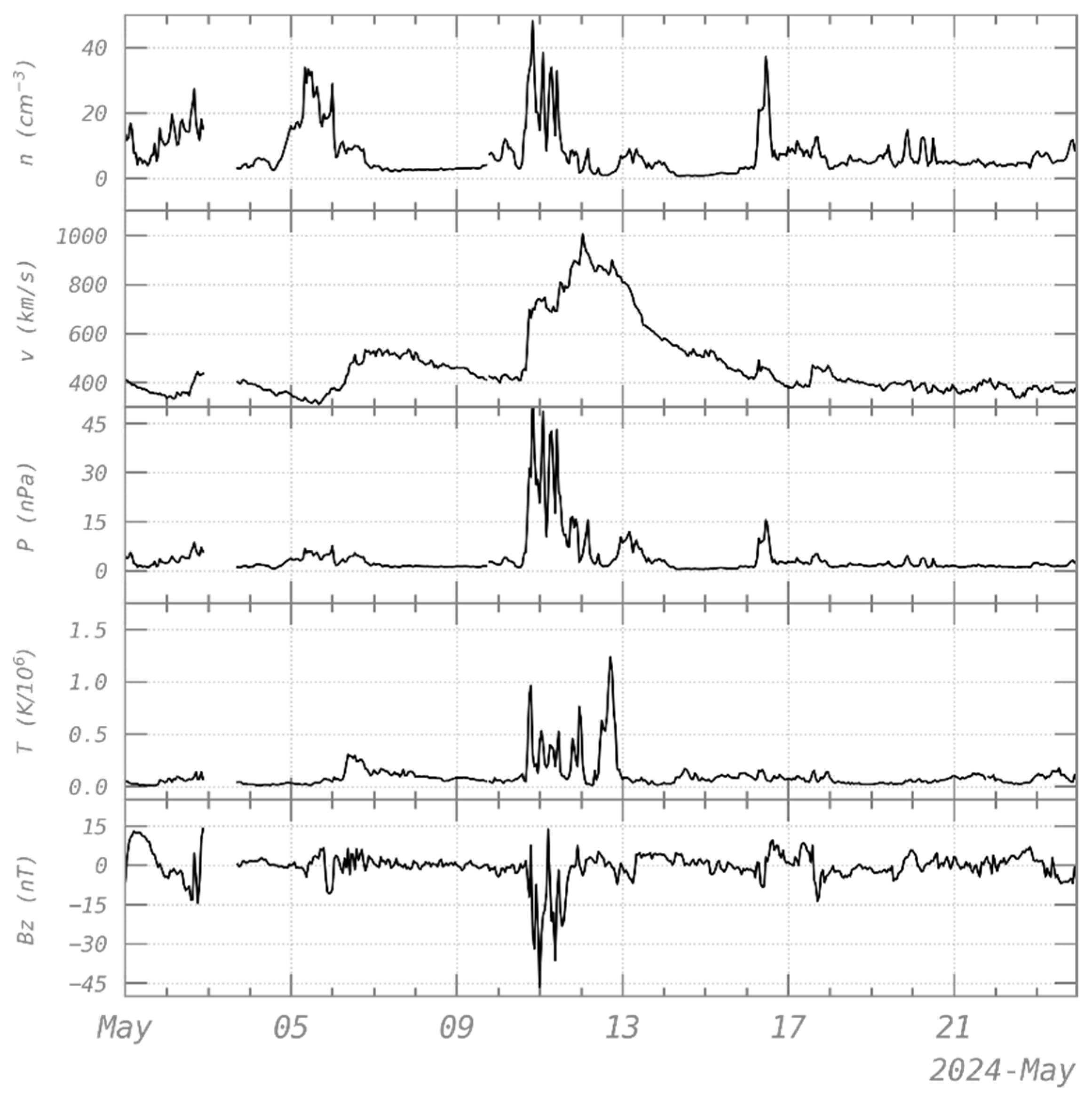
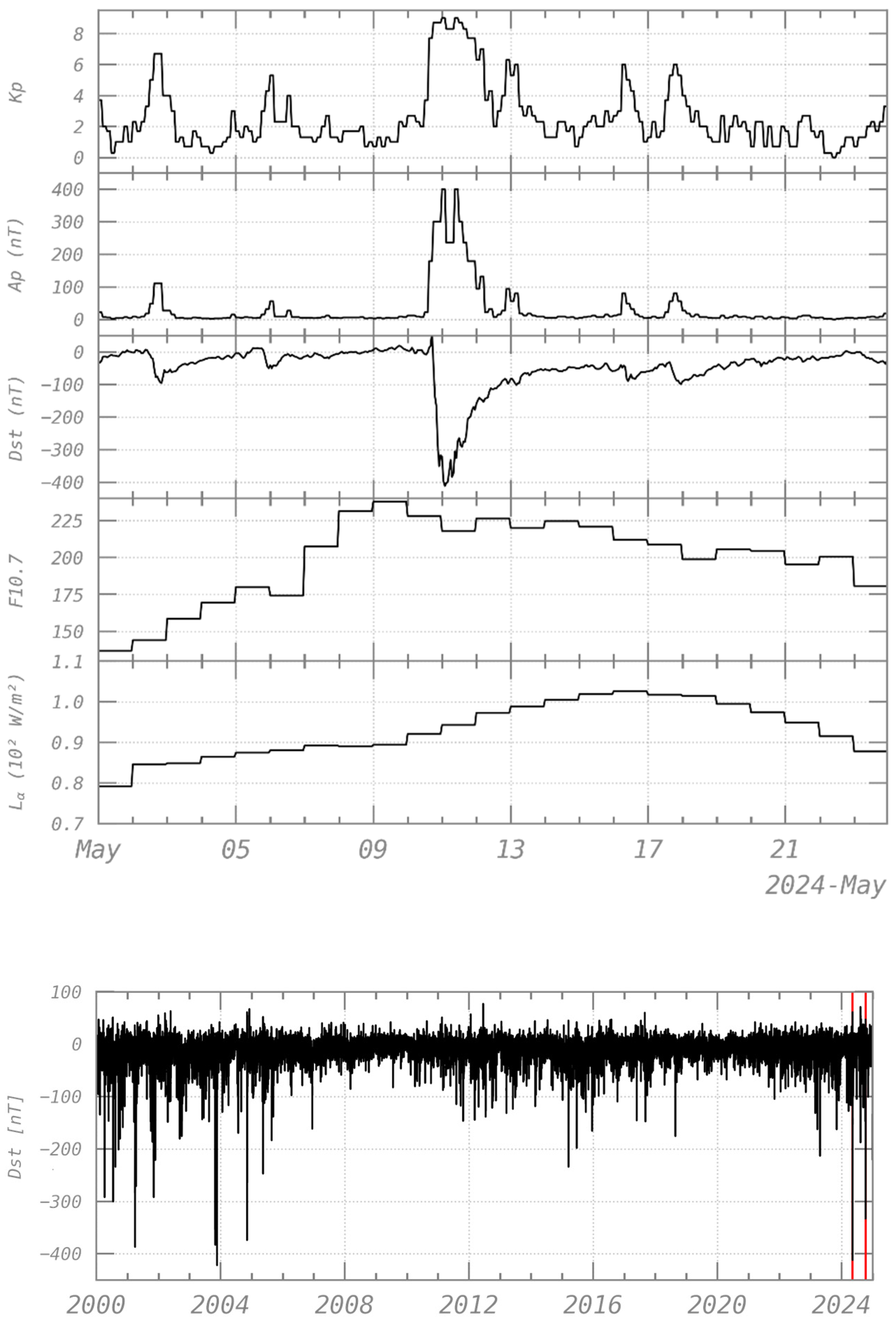
2.1. Solar Wind and Geomagnetic Indices

OMNI is a multi-source data portal of the near-Earth solar wind’s magnetic field and plasma parameters provided by NASA. We use it to obtain the solar wind parameters measured at 1 Astronomy Unit (UA) (i.e., the average distance between the Sun and Earth) from in situ spacecraft and the geomagnetic activity indices.

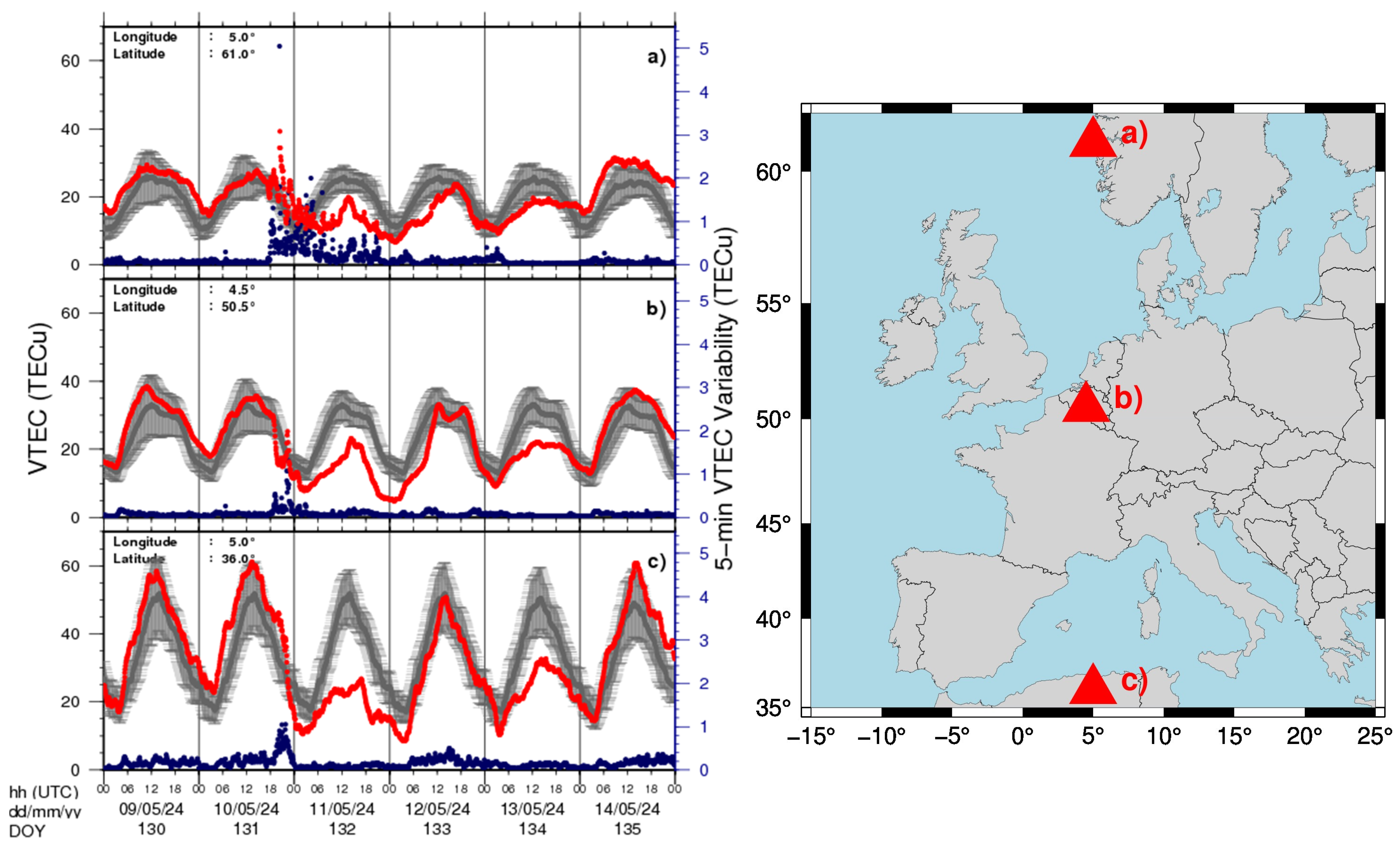
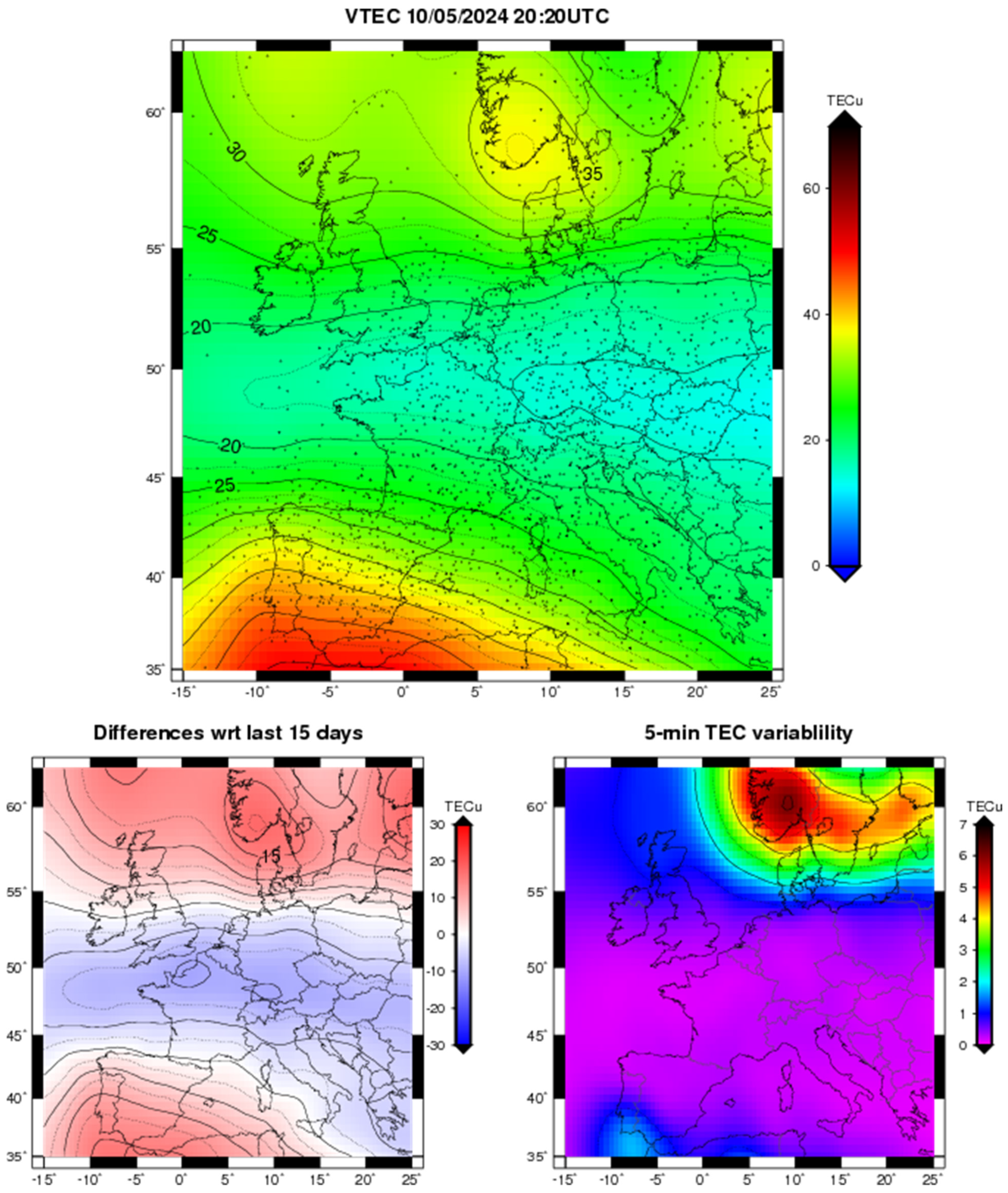
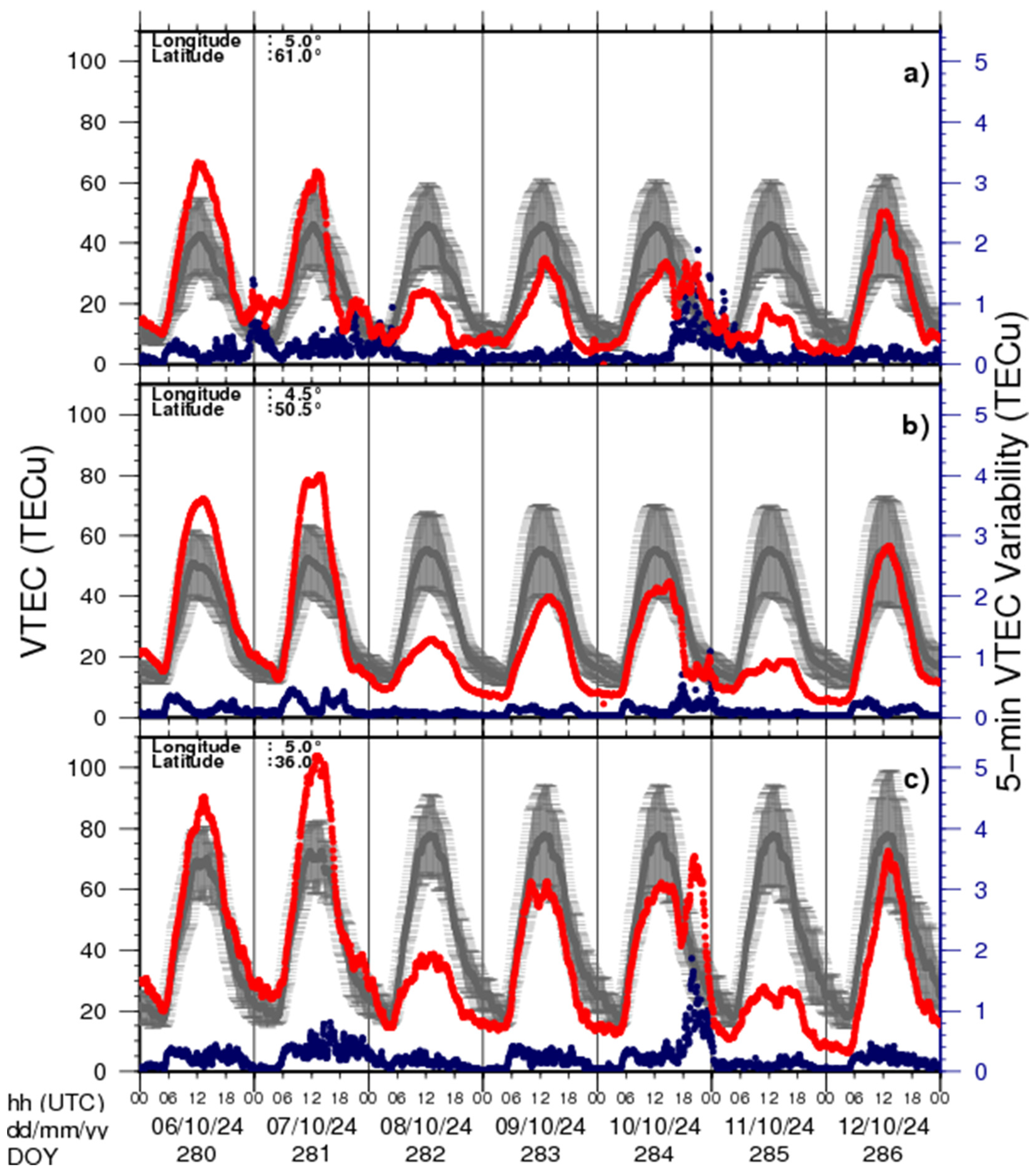
2.2. Vertical Total Electron Content VTEC

One of the key parameters used to characterize ionospheric conditions is the vertical total electron content (VTEC). The TEC represents the total number of free electrons integrated along the ray path between a satellite of the Global Navigation Satellite System (GNSS) located at an altitude of 19,100 km to 23,300 km (thus, a radial distance from the centre of the Earth of approximately 4 Earth radii, Re) and the receiver on the ground. The TEC is measured in TEC units (TECu), where 1 TECu = 10¹⁶ electrons/m². The VTEC is the vertical projection of TEC at the Ionospheric Pierce Point (IPP), which intersects above the electron density peak at a 450 km height.

The VTEC is directly related to the GNSS signal propagation delay caused by the ionosphere. These ionospheric conditions are continuously monitored by the STCE in Brussels based on the GNSS observations of the EUREF Permanent Network (EPN) [21] and processed using the ROB-IONO software [22].

Real-time GNSS data from ~150 stations (GPS + Galileo + GLONASS) are used to estimate the VTEC at the IPP every 30 s, covering a 5 min time span. This approach provides extensive spatial and temporal coverage for monitoring the ionosphere state. For each 5 min interval, median VTECs at the IPP for each satellite–receiver pair are estimated along with their standard deviation and are then interpolated to produce VTEC and VTEC variability maps above Europe. The methodology for producing these maps and their validation against widely used post-processed Global Ionospheric Maps such as IGS and ESA, with mean differences of 1.3 ± 0.9 and 0.4 ± 1.6 TECu, respectively, are detailed in [22].

The VTEC time series provided in this paper are extracted from these maps at three locations:

(a)

In the northern part of Europe (61° N, 5° E);

(b)

Above Brussels, in mid-latitude Europe (50.5° N, 4.5° E);

(c)

In North Africa (36° N, 5° E).

The expected VTEC at each location corresponds to the median of the 15 previous ones for the same local time.

2.3. Ionosonde Observations

Ionosondes employ high frequency (HF) radio transmissions of various frequencies to determine the electron density profile above the instrument. Frequencies below the plasma frequency $\omega =\sqrt{{\displaystyle \frac{N_e{e}^2}{{\epsilon }_{0}m}}}$ (where e is the electron charge, m is its mass, and ε₀ is the permittivity of free space) are reflected by the plasma in the ionosphere. Therefore, the electron density profile $N_e\left(h\right)$ can be reconstructed from the reflection of a range of different frequencies. The main limitation of this technique is that it allows observations only up to the height of the greatest electron density. This altitude varies significantly both during quiet conditions and as a result of particular disturbances such as geomagnetic storms.

In the present study, we use data from three ionosondes in Europe (JR055, DB049, and EB040), at different latitudes, as well as two ionosondes in other longitude sectors: IC437 in South Korea and MHJ45 in the USA. Ionograms were obtained from the DIDBase of the GIRO repository [23]. This allows us to compare the storm effects at different latitudes as well as the effects of the local time at the onset of the event. The coordinates of the observatories are listed in

Table 1. Ionosondes from which data are used.

Name (Country)	URSI Code	Latitude	Longitude
Juliusruh (Germany)	JR055	54.60° N	13.40° E
Dourbes (Belgium)	DB049	50.10° N	4.60° E
Roquetes (Spain)	EB040	40.80° N	0.50° E
Millstone Hill (USA)	MHJ45	42.60° N	288.50° E
I-Cheon (South Korea)	IC437	37.14° N	127.54° E

. Each of these observatories uses a similar Digisonde DPS-4D ionosonde and produces regular soundings of the ionosphere at intervals of 5 (for the European observatories) or 7.5 min (for the American and South Korean observatories). All ionograms were manually inspected in order to derive the characteristics of the various layers (here, we use the critical frequencies foF₁ and foF₂ of the two F region density peaks), only retaining the data points which could be obtained reliably according to the standard URSI (International Union of Radio Science) rules.

The exceptional ionospheric conditions during the events analyzed here cause some particular difficulties in the interpretation of the ionograms. There are three reasons for occasional gaps in the time series of the critical frequencies. First, during the nighttime, the spreading of the F₂ trace is observed (see the left panel of Figure 1 for an example). This can render it impossible to accurately determine the critical frequency foF₂. During the first night of the 11 May storm, there were also sporadic E layers observed, produced by particle impacts (which are associated with the visible auroras seen at those same times even at low latitudes). An example of this is shown in Figure 1 on the right. In this example, the Es layer extends to above 4 MHz, making it impossible to detect the depleted F layer above.

Finally, there are some gaps in the data related to the absorption of the ionosonde signals in the D region of the ionosphere due to an increased X-ray flux or polar and auroral absorption (the latter mostly affects data from the Millstone Hill observatory). On 11 May 2024, there was an X5.89 flare peaking at 01:23 UTC (Universal Time Coordinated) and an X1.54 flare peaking at 11:44 UTC. In addition, during the period of interest, there were some M-class flares as well. For most of 11 May, even the minima of the X-ray flux remained above the level of an M1 flare. Depending on the signal-to-noise ratio usually obtained by the different ionosondes, and the local time at each during the flares, this absorption in the lower ionosphere results in gaps in the observation of the F layer.

2.4. Plasmasphere Model and Data

The Belgian SWIFF plasmasphere model (BSPM) is a 3D kinetic semi-empirical model of the plasmasphere [24], coupled to the ionosphere [25]. It has recently been improved to take into account the most recently identified relevant physical processes [20]. It can be run for any date to obtain for every hour the number density and temperature of the electrons and protons inside and outside the plasmasphere, as well as the position of the plasmapause, as a function of the geomagnetic activity driven by the Kp index. The model uses the kinetic approach for the particle densities and the mechanism of quasi-interchange instability for the formation of the plasmapause. The density in the plasma trough region has recently been improved using observations of Van Allen Probes [26]. The results of the plasmasphere model have been compared to NASA’s IMAGE mission (2000–2005) global EUV images of the plasmasphere [27], Cluster [28] and Themis [29], among others, allowing the validation of the plasmasphere erosion and dynamical evolution. The most recent version has been made available on the PITHIA [30] platform: https://esc.pithia.eu/ (accessed on 5 November 2024).

Moreover, the magnetic and plasma observations of the low-Earth orbiting Swarm satellites allow us to derive the midnight plasmapause [31]. Launched on 22 November 2013 into a near-polar low-Earth orbit (LEO), Swarm is a constellation of three identical satellites operated by the European Space Agency (ESA) with the purpose of mapping Earth’s magnetic field [32]. The initial altitude of the satellite pair Swarm A and Swarm C was about 490 km in April 2014, and it was about 510 km for Swarm B, and both orbit altitudes do slowly decay with time. Based on in situ electron density and temperature [33], GPS-derived TEC, and auroral field-aligned current observations at the Swarm satellites, new Swarm products have recently been developed to characterize plasmapause-related boundaries in the topside ionosphere. This product also includes a plasmapause index, a proxy for the midnight plasmapause position. This index is derived from Swarm observations similarly to the ones described in [34].

3. Mother’s Day Storm: 10–11 May 2024

3.1. Observed Solar Wind and Geomagnetic Indices

An exceptionally strong geomagnetic storm occurred during the night from 10 to 11 May 2024, with auroras observed around the world [2,3,4]. This was the strongest storm of the last twenty years with a minimum Disturbance Storm Time index of Dst < −400 nT (see bottom panel of Figure 3). Due to the varying speeds and quick succession of different coronal mass ejections (CMEs) coming from the active region NOAA 13664, several of them merged and interacted as they travelled through the interplanetary medium, leading to enhanced effects in the Earth’s space environment [1]. These CMEs were associated with the X2.2 flare on 9 May and three X1 flares on 8 May.

The characteristics of the solar wind when it reached 1 AU, obtained from OMNI, are shown in Figure 2. The bulk velocity of the solar particles reached more than 1000 km/s (see Figure 2, 2nd panel), and peaks of high temperature > 10⁶ K were observed (panel 4). The high-density peak (panel 1) at the arrival of the hot plasma shows the apparition of a shock. The pressure (panel 3) combines the density and velocity effects and determines the position of the magnetopause. The downward peak of the Z component of the Interplanetary Magnetic Field Bz (panel 5) shows a southward direction that can explain the strong answer of the terrestrial magnetic field [35].

The arrival time of enhanced solar plasma at 1 AU with regard to density, velocity, and pressure is 10 May 2024 at 17:07 UT. It directly caused the sudden commencement of the strong geomagnetic storm (see Figure 3), followed by the main phase, when the Dst index decreased down to a minimum value of −412 nT (see panel 3) in the night of 11 May, and the planetary geomagnetic activity index Kp increased to the maximum value of 9 (panel 1). The geomagnetic activity indices Kp, Ap (in nanotesla) that reached 400 nT (see panel 2), and Dst (also in nT) are illustrated in Figure 3, together with the F10.7 solar radio flux at 10.7 cm (panel 4) and the intensity of the Lyman alpha line in the solar spectrum (panel 5) that are daily solar activity indices.

The bottom panel of Figure 3 illustrates the Dst index from 1 January 2000 to 31 January 2025. The two analyzed events are indicated by the red vertical lines. This panel clearly shows that the last event with Dst < −400 nT appeared in November 2003 (known as the Halloween Day storm [1]) and that the intensity of the geomagnetic storm of October 2024 was not seen since November 2004.

3.2. Ionospheric Vertical Total Electron Content

Figure 4 shows the time series of the VTEC (in red), the expected VTEC, i.e., the 15 previous days median (in grey, with standard variation), and the 5 min VTEC variability (in blue) in the north of Europe, middle of Europe (Brussels) and more southward (north of Africa). The three near-real-time VTEC time series showed abnormal variations during the night of 10 to 11 May 2024, followed by a long depletion in VTEC until 12 May 2024. This is due to the strong CME impact detected during the afternoon of 10 May. By comparing with Figure 3, these VTEC fluctuations (high variations during the storm and long depletion after) cannot be explained by variations in F10.7 during these days.

Consequently, the geomagnetic storm had a strong impact on the ionospheric electron content, with sudden increases and decreases of 20 TECu from 18:00 UTC 10 May to 12:00 UTC 11 May in the north of Europe. At mid-latitude, the VTEC tends to decrease starting at 18:50 UTC, with a minimum of −10 TECu, with respect to the expected quiet ionosphere, and with a sudden peak of an increase of 8 TECu (with respect to the quiet ionosphere) at 22:20 UTC. At the same time, at a low latitude, the VTEC starts to decrease with respect to the quiet ionosphere. For both mid- and low latitudes, the VTEC variability also remains high, until midnight on 11th May. These VTEC variations and rapid variability at these three latitudes are due to the injection of the particles associated with the storm and leading to the occurrence of auroras at unusually low latitudes.

The maximum variability in the VTEC is observed at 20:20 UTC (see Figure 5).

In Figure 5, it can be observed that an increase in TEC with respect to the quiet ionosphere occurs at high and low latitudes, while this is negative at mid-latitude. Over Scandinavia, the VTEC variability reached a maximum of 5 TECu for a 5 min interval at 20:20 UTC. This could be linked with the height values in the rate of TEC change index (ROTI) observed in [2], supporting the fluctuations, implying disturbances in GNSS applications.

The other effect of the storm is the depletion of the VTEC down to 30 TECu at low latitudes until 12 May around 05:00 UTC. As mentioned in [36,37], the persisting depletion in TEC a few days after the onset is due to the contraction of the plasmasphere, implying disturbances in the thermospheric circulation and a chemical loss of ionization in the ionosphere. This contraction of the plasmasphere is coherent with the observation in Figure 9 Section 3.4 of the present paper.

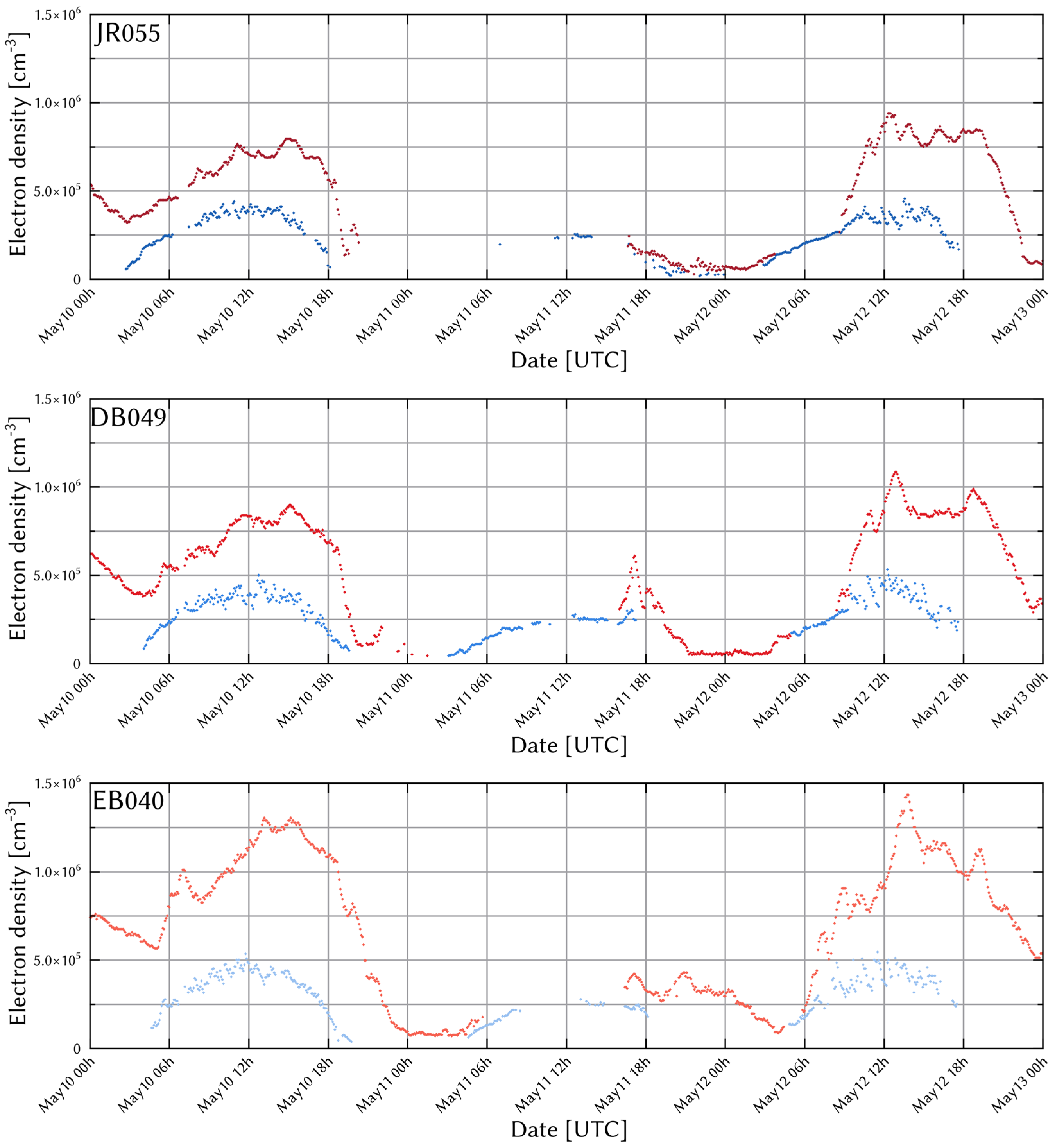
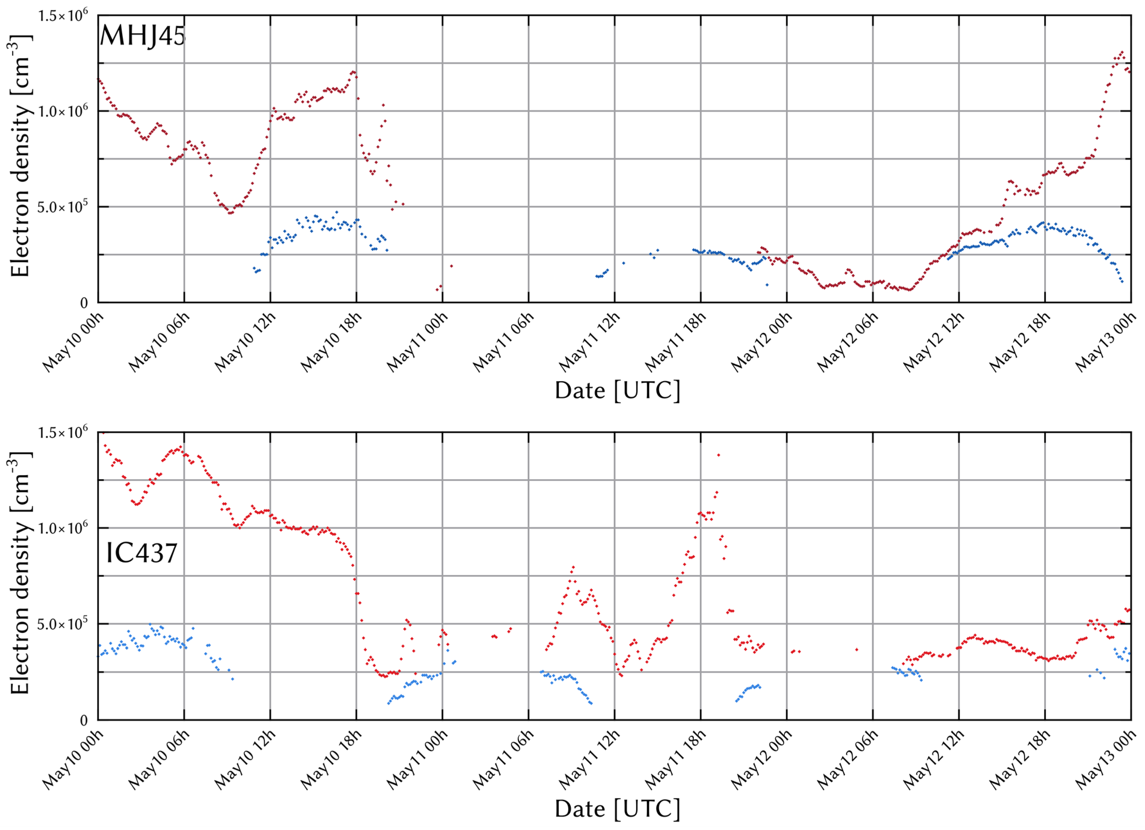
3.3. Ionosonde Observations

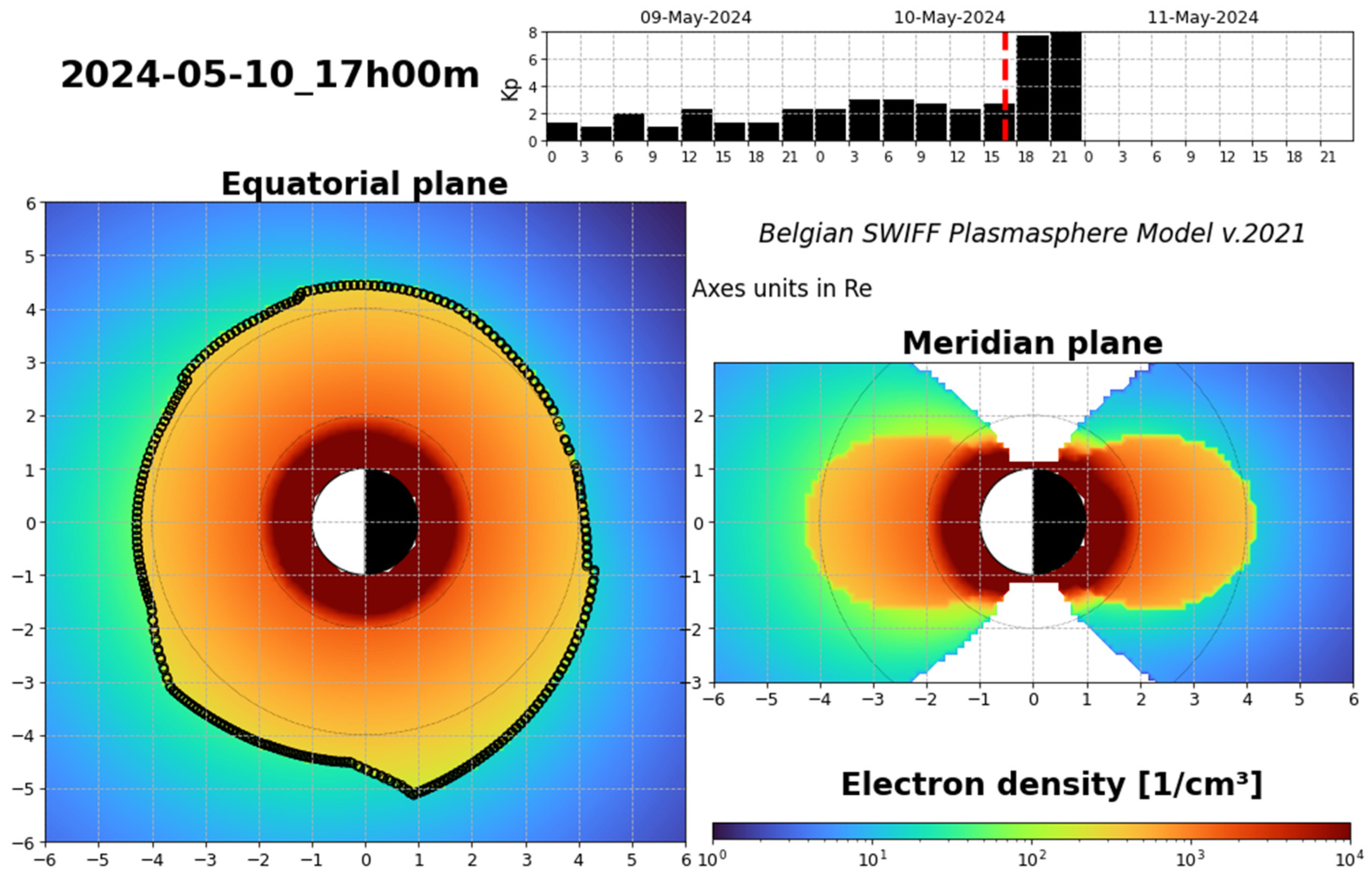
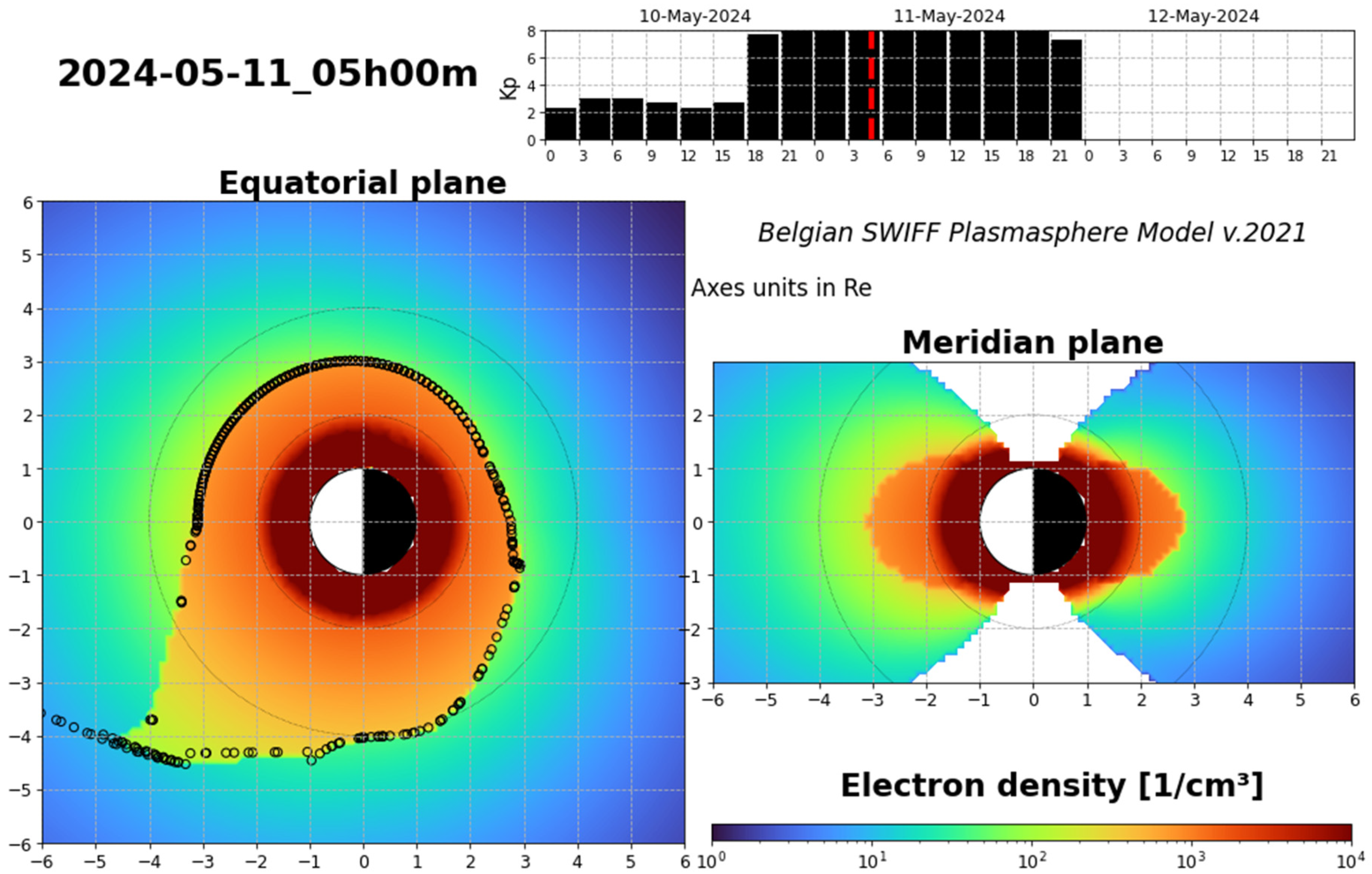
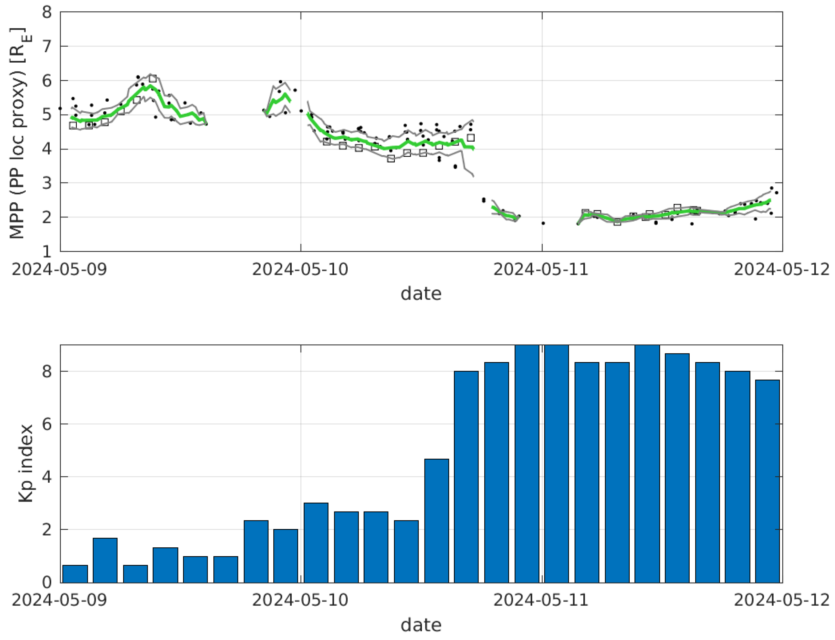
Figure 6 shows the peak electron densities for the F₁ (in blue) and F₂ (in red) layers for the three European ionosondes for a three-day period covering 10 to 12 May 2024. The E layer was found to be not affected by the geomagnetic storm. This is to be expected, because the E layer is known to be driven entirely by solar irradiance.

At the onset of the storm, a very rapid depletion of the F₂ layer density can be observed. The depletion appears to be more rapid at the higher latitudes, although of course the peak density before the storm is lower at higher latitudes as well. For the most part of 11 May, the F₂ layer was not detected, because the electron density in the F₂ region was lower than in the F₁ layer and thus not visible to the ionosondes. This is referred to as the “G-condition” in the ionosonde community and is often seen during major storms (see for instance [38] for some recent examples). The density of the F₁ layer is also seen to be lower than during the quiet day before the storm, but the depletion is much less severe than in the F₂ layer because transport processes and chemical changes are less important at the F₁ layer altitude compared to the influence of solar irradiance.

The strong depletion of the F region lasts throughout 11 May and the morning of 12 May. The reappearance of the F₂ layer on 12 May and its return to a quiet time peak density is almost as rapid as the depletion at the onset of the event. This indicates that the refilling of the F₂ layer was very quick. It is also evident that this refilling occurred earlier at the EB040 observatory, which is at the lower latitude. Here, the F₂ layer was detected again around 06 UTC. At the DB049 and JR055 ionosondes at higher latitudes, the F₂ layer was not detected until around 09 UTC, and the peak density reached its climatological values only around noon.

Although the reappearance of the F₂ layer happens earlier at lower latitudes, it can be seen that the peaks of the highest electron density reached on 12 May occur earlier at the highest latitude. The highest density is seen on 12 May at 12:20 UTC by JR055, at 12:50 UTC by DB049, and at 13:45 UTC by EB040. This seems to indicate large-scale travelling ionospheric disturbances (LSTIDs) moving from the auroral region to lower latitudes. Such LSTIDs are usually seen during the beginning of a storm (e.g., [39]) but seem to also occur here at the time of the refilling of the F₂ layer.

Figure 7 shows the critical frequencies of the F₁ and F₂ layers for the Millstone Hill (MHJ45) and I-Cheon (IC437) ionosondes. The behaviour of foF₂ at MHJ45 (top panel) can be seen to be very similar to what was observed by the European ionosondes (see Figure 6). There is a sudden depletion starting at 18:00 UTC on 10 May and lasting until 12 May. G-condition was observed for the entirety of 11 May. Around 09:00 UTC on 12 May, there is a sudden increase again in the F₂ layer density. At MHJ45, this corresponds to the normal morning-time density increase (as is evident by comparing with the same time on 10 May, which is still before the onset of the storm). This sudden refilling thus occurs at the same time in the European and American sectors, despite the local time difference. The pattern of the F₁ layer at MHJ45 is of course delayed in time compared to the European observatories as a result of this local time difference.

The observations at IC437 (bottom panel of Figure 7) show a different pattern. A sudden depletion at the storm onset is again evident, but at this location, 18:00 UTC corresponds to nighttime. During the local daytime on the two succeeding days, there are multiple gaps in the data due to the various difficulties explained above. Nevertheless, from those ionograms that could reliably be scaled, it is clear that severe depletion persisted throughout these days, and even during the local nighttime on 12 May—the end of the time series shown in the Figure—the electron density has clearly not recovered yet to the quiet-time level seen before the storm onset. The peaks in foF₂ seen during the local nighttime on 11 May correspond to periods of strong spread-F associated with auroral oval structures expanding to the latitude of this observatory.

During the main phase of the storm, the electron density and the height of the F region decreased and increased, respectively, indicating an upward displacement of the ionosphere (depression and uplift) and irregularities (plasma bubbles) due to the stable aurora red arc convergence of low- and high-latitude effects.

The electron density in the F₂ layer decreased due to the expansion of the atmosphere that modified the recombination time of the ionized particles. During the strong post-storm depletion, F₂ disappeared behind the F₁ layer. The strong spread-F initiated during the main phase was still present during the next nights and caused the scintillation of the satellite signals. After the arrival of the CME, the electron density decreased and remained significantly lower than during the quiet days for more than a full day, including during the recovery phase of the geomagnetic storm. This meant that for high-frequency (HF) communication, the portion of higher HF frequencies was not available for communication, and so several advisories were sent to civil aviation via PECASUS (https://pecasus.eu/, accessed on 12 May 2024) to warn for this so-called post-storm depression [40].

Unusually high spatially distributed values of the rate of TEC change index (ROTI) were detected on the nights of 10 and 11 May [2]. The ROTI enhancements on 10 May might be linked to stable auroral red arcs and an equatorward displacement of the main ionospheric trough. Instead, the ROTI enhancements on 11 May might be triggered by a joint action of low-latitude plasma pushed poleward by the pre-reversal enhancement in the post-sunset hours and wave-like perturbations propagating from the north.

3.4. Plasmasphere

While ionosonde measurements are not affected by the density of electrons in the plasmasphere, this is not the case for VTEC. The sudden but short increase in density observed at the onset of the storm, in VTEC but not by the ionosondes, indicates that this additional ionization appears above the F₂ peak. The plasmaspheric density is thus very important to determine. The sharp density decrease measured by both techniques shows that it already takes place at low altitudes in the F layer. Considering also the plasmasphere erosion appearing during storms (e.g., [41]), VTEC observations allow us to determine the plasmaspheric part in comparison to the ionospheric reduction.

The plasmasphere is the extension at the low and middle latitude of the ionosphere to a higher altitude [42], and its erosion can also explain the reduction in VTEC during and after the storm. Indeed, the extend of the plasmasphere is strongly reduced after storms, with a sharp plasmapause appearing at lower radial distances, as is illustrated in Figure 8 using the BSPM plasmasphere–ionosphere model [20]. The top panel shows the extended plasmasphere (orange region with high electron density) before the storm, with an average plasmapause position above 4 Re at all Magnetic Local Times (MLTs). The plasmasphere is seen in the geomagnetic equatorial plane (left panel) and in the meridian plane (right panel), with the Sun (thus noon 12:00 MLT) on the left.

The bottom panels show the eroded plasmasphere after the storm, which is very strong due to the Kp reaching the maximum value of 9. The new plasmapause is located around 3 Re on average but is as low as 2.3 Re in the post-midnight sector and as high as 5 Re at the endpoint of the plume in the afternoon MLT sector. The plume co-rotates with the Earth after its formation. It takes typically 2 or 3 days after the storm to progressively refill the outer shells of the plasmasphere [20].

The plasmasphere erosion after the storm can thus at least partially contribute to the observed VTEC. When the plasmapause comes closer to the Earth in the equatorial plane (see Figure 8 left bottom panel), the ionospheric trough also appears at lower latitudes (see right bottom panel) due to the motion of the particles along the magnetic field lines [25].

The midnight plasmapause proxy derived from the magnetic and plasma observation of the low-Earth orbiting Swarm satellites also confirms a very low plasmapause after 11 May 2024 reaching less than 2 Re, as illustrated in Figure 9 (top panel) with the Kp index (bottom panel). Such plasmapauses lower than 2 Re are very rare. The green line corresponds to the midnight plasmapause position, and the black lines give the position ± the standard variation. The squares correspond to the Swarm plasmapause observations. The plasmapause is directly related to the mid-latitude ionospheric trough (MIT) observed by Swarm [31]. The dots show the plasmapause index, based on the L value distance between the small-scale field-aligned current boundary and the MIT minimum.

The position of the plasmapause is crucial because different waves are generated inside and outside the plasmasphere, and they affect the particles trapped in the radiation belts [43,44]. Several unusual electron belts were observed after the 11 May 2024 geomagnetic storm, as well as a strong increase in the protons from 9.5 to 13 MeV trapped in the south part of the South Atlantic Anomaly [1].

4. Comparison with Event of 10 to 11 October 2024

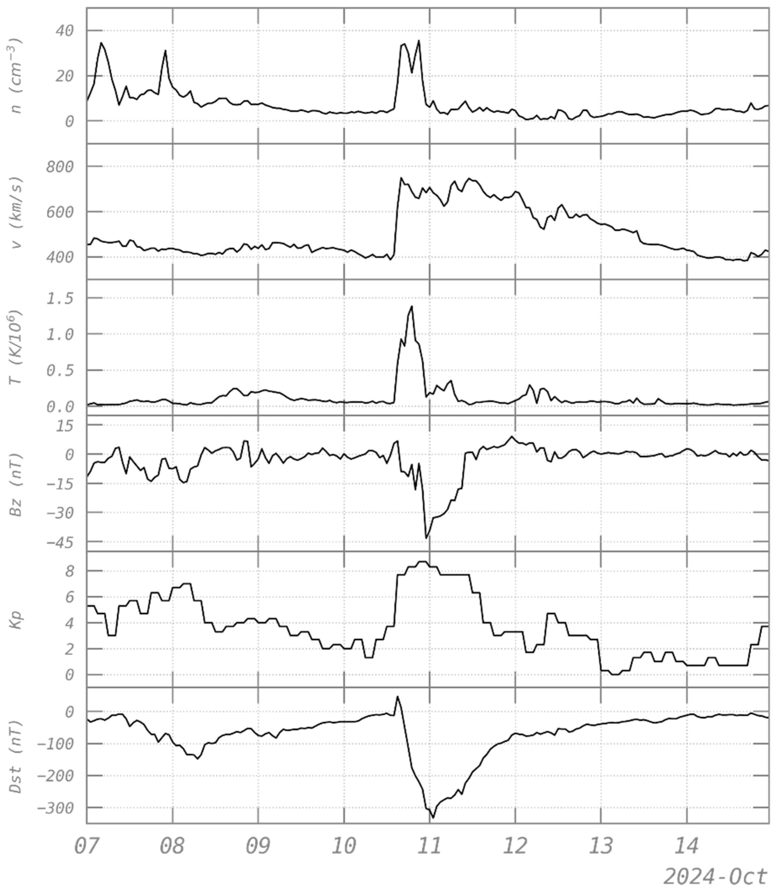
4.1. Solar Wind and Geomagnetic Activity Indices

The second most important storm (so far) of the present solar cycle 25 started on 10 October 2024 and reached a minimum of Dst = −335 nT on 11 October 2024. It was preceded by another storm with a minimum of Dst = −153 nT on 8 October, as illustrated in Figure 10 (bottom panel) together with the Kp index (5th panel) and the solar wind characteristics that generated these storms: density (1st panel), bulk speed (2nd panel), and temperature (3rd panel). The 8 October storm, associated with an X9 flare on 3 October, is mainly due to the arrival of high-density but low-energy particles, while the 11 October storm (associated with an X1.8 flare on 9 October and an X2.1 flare on 7 October) is due to a density peak of energetic particles, as can be seen in the temperature and bulk speed observations. The velocity of the solar wind particles exceeded 700 km/s for this last event. The negative Bz of the interplanetary magnetic field (see 4th panel) explains the high geomagnetic perturbations induced on the terrestrial magnetosphere.

In Figure 10, the arrival of the energetic solar wind particles initiating the strong geomagnetic storm is well visible in the evening of 10 October 2024 (Dst = −335 nT, Kp = 9−), preceded by a smaller event (Dst = −153 nT, Kp = 7) starting on 7 October due to a peak of solar wind density. Both give effects visible in the ionosphere.

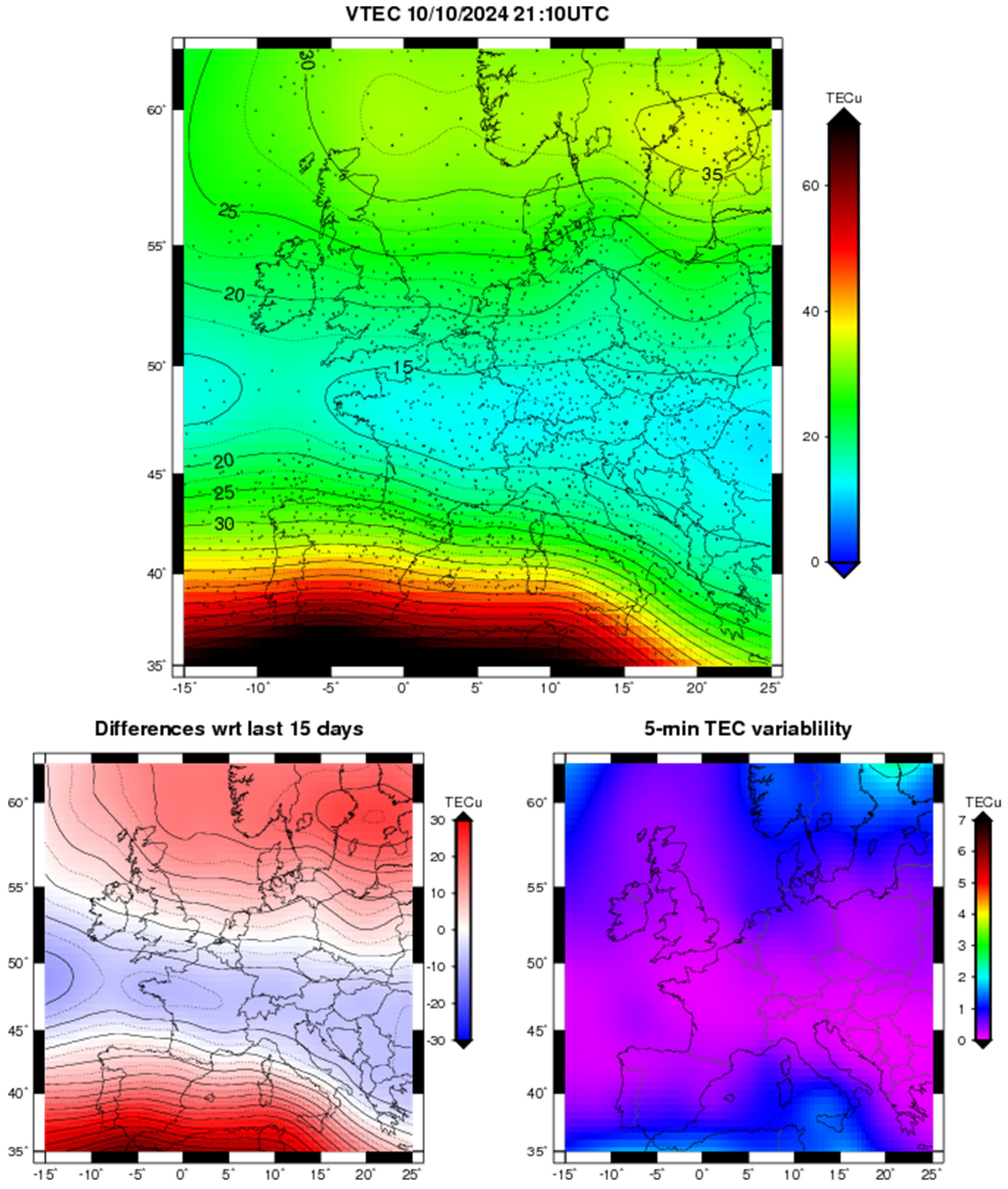
4.2. Ionospheric VTEC

Figure 11 shows that the two geomagnetic storms led, at the three different latitudes, to high variations in VTEC during the main phase of the storm (see red line). The VTEC variability reaches 2 TECu/5 min in the north and south. However, the storm impact is different in the southern location. Indeed, while the variability is high, the VTEC does not show rapid variations, but a smooth abnormal VTEC increase (red line, Figure 11c) compared to the expected behaviour with a maximum of differences at 21:10 UTC up to +35 TECu.

Figure 12 shows the state of the ionosphere during this maximal VTEC difference observed in the southern location at a low latitude. As we can see, the VTEC observed is more than 30 TECu higher than the expected values. This is not seen in the ionosonde electron density observed by the ionosonde in Spain (see Figure 13, EB040), where no significant increase is observed. This difference between VTEC and electron density from ionosonde can be interpreted as an increase in the electron density above the F₂ layer up to the plasmapause. This density peak is followed by a sharp decrease, leading to a value lower than the averaged density of the quiet times (grey line) during the night and the full next day and night. This after-storm depletion stands ~1.5 days (until the 12th 08:00 UTC) as seen for the Mother’s Day storm, with a minimum of −55 TECu in the low latitude on 11 May at 13:50 UTC.

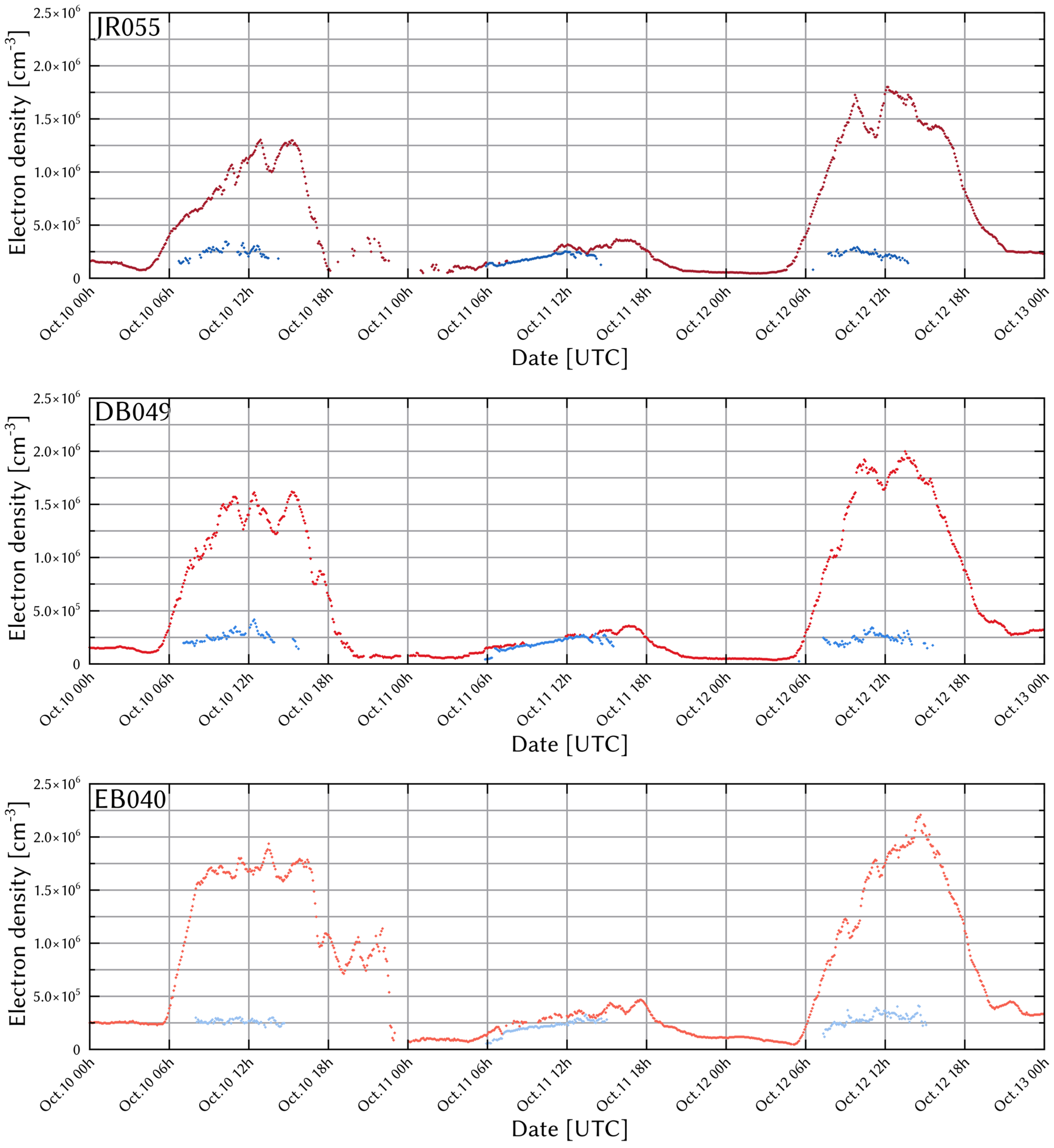
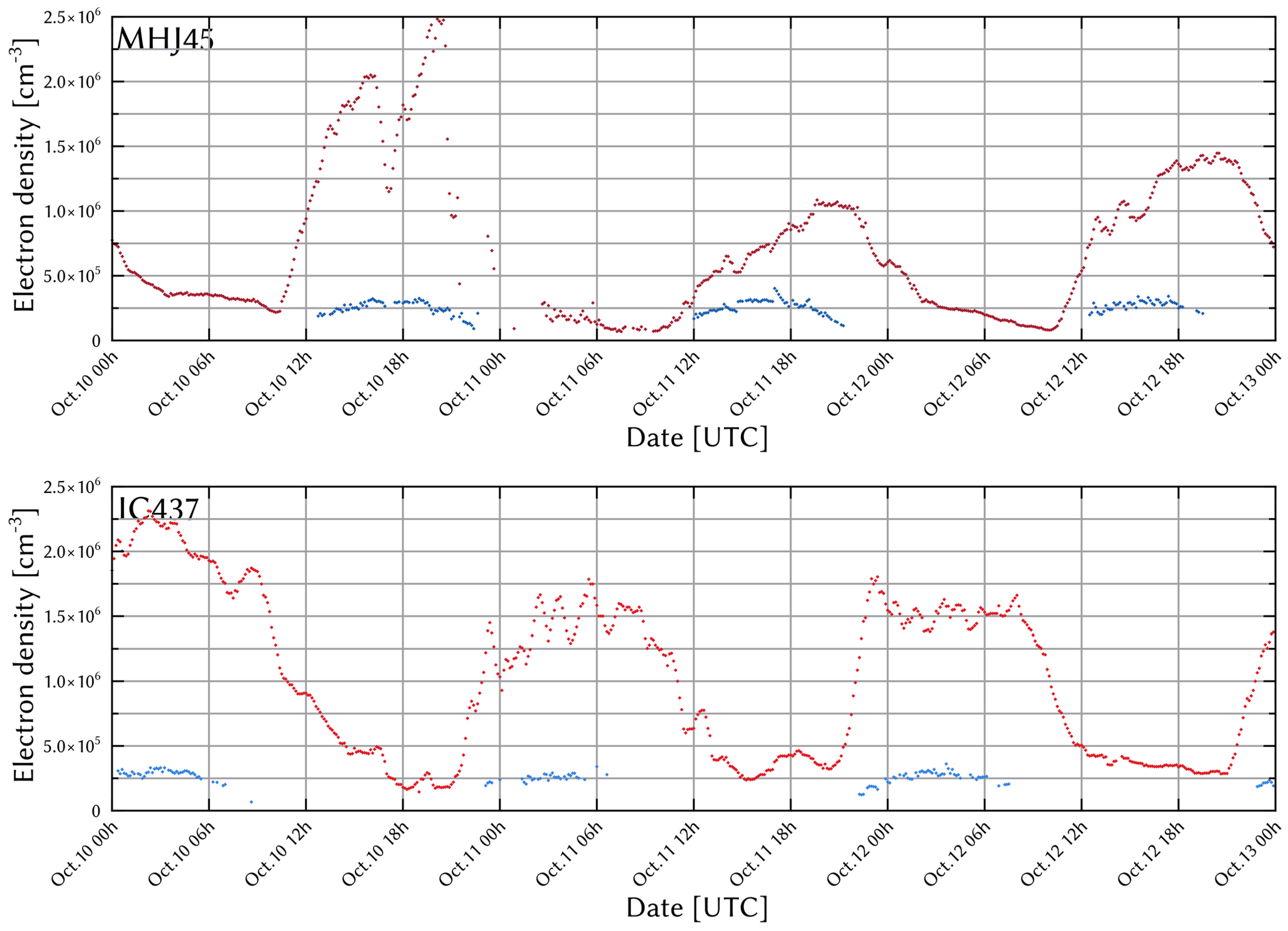
4.3. Ionosonde Observations

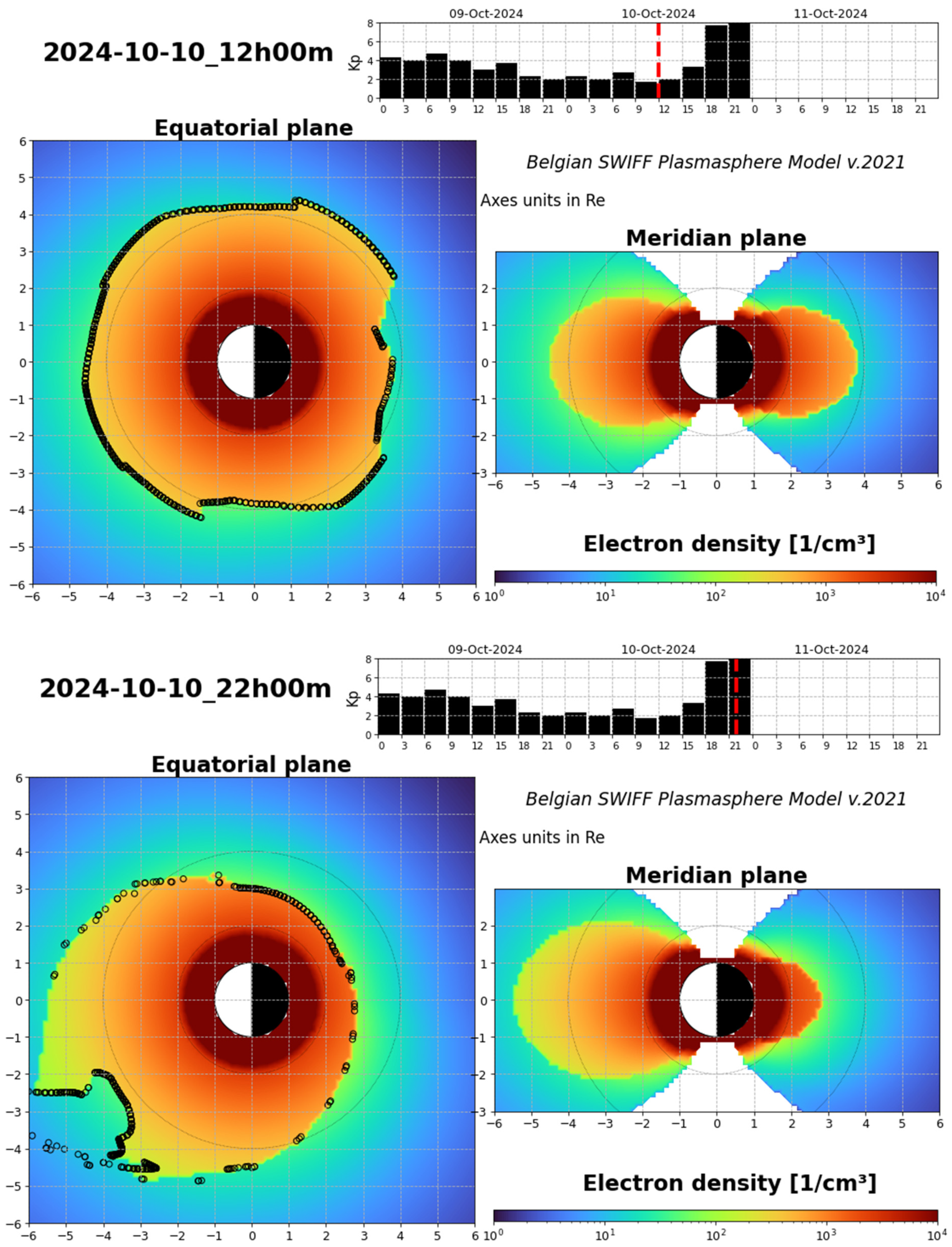
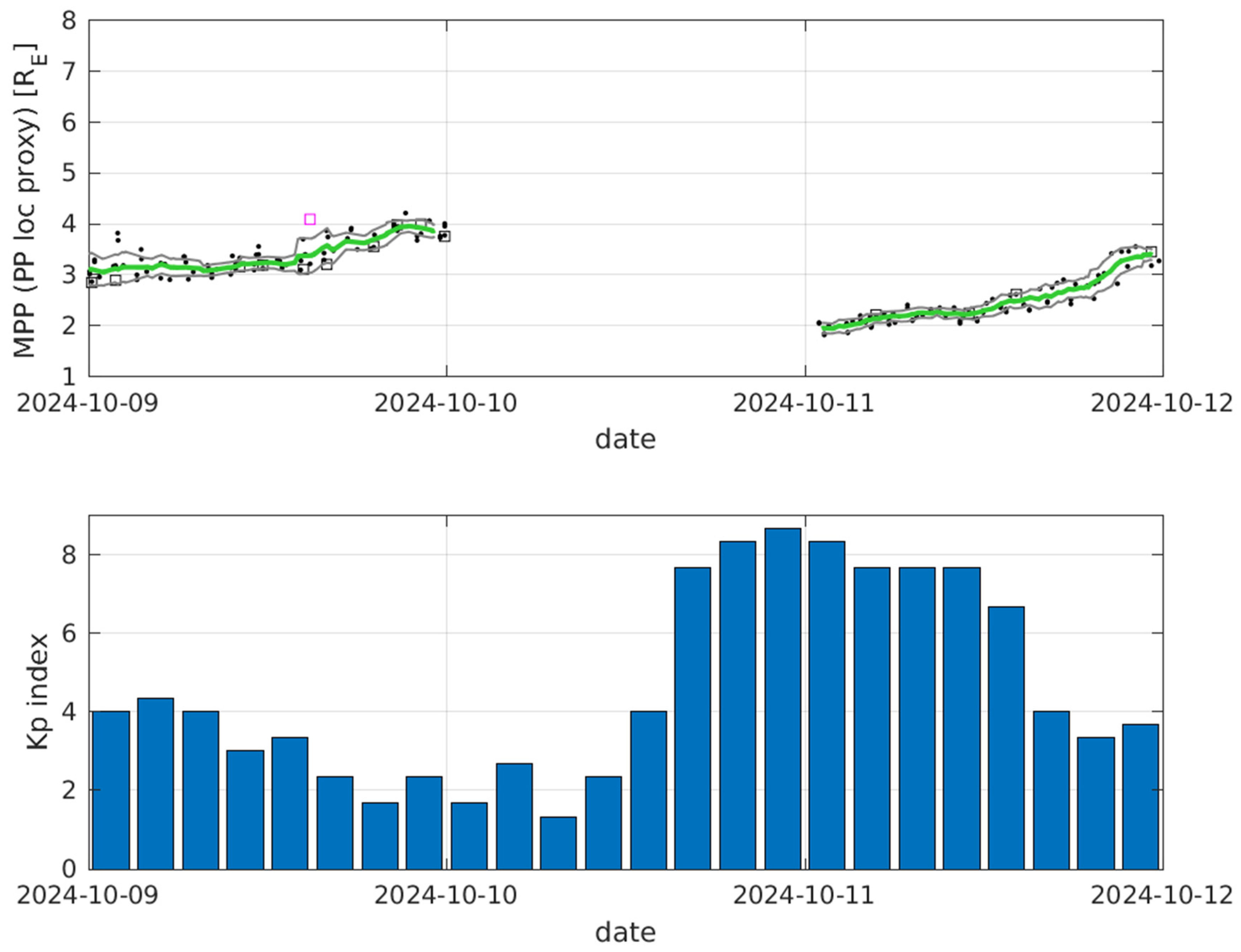
Figure 13 shows the equivalent observations as seen in Figure 6 but for the storm of 11 October 2024. The climatological conditions in October are different from those during the May event. The foF₁ peak is not as pronounced in October as it is in May. On the other hand, the foF₂ is slightly higher during the October event than during the May storm.

Note that there are again some gaps in the time series, in particular during the night of the storm at the highest latitude observatory (JR055). These are primarily due to the presence of particle-induced sporadic layers precluding observing the F region of the ionosphere. Blanketing of the observations by regular Es layers is not important for this event as such layers are more rarely present at these observatories in October as compared to May.

At the onset of the storm, a steep drop in the F₂ layer density can again be observed, indicating the sudden depletion of the ionospheric plasma. The main phase and recovery, on the other hand, look different for this storm. The cases of G-condition being observed are limited, in particular in the southernmost observatory, and the background conditions were restored already in the morning of 12 October.

Figure 14 shows the critical frequencies observed by the American and Korean ionosondes. Once again, it should be noted that the F₁ peak is not as clearly observed as during the May event, and that the foF₂ values are slightly higher. At these observatories, no G-condition was observed. This is due to the local time of the onset of the storm. As can be seen from Figure 13, the period of the G-condition observed by the European ionosondes was relatively short, compared to what was seen during the May event, from around 06:00 to around 12:00 UTC at JR055. This coincides with a period when no F₁ layer is detected at MHJ45 and IC437, so there can be no G-condition.

Some depletion of the F₂ layer during the first day after the storm can still be seen at both observatories though. In both cases, the foF₂ at the end of the period has not yet recovered entirely to the values seen before the storm. In addition, the presence of large-scale travelling ionospheric disturbances can be seen. Especially during 11 October at IC437, there are periodic oscillations evident in foF₂.

4.4. Plasmasphere

The BSPM shows that on 10 October 2024 12:00 UT, before the superstorm, the plasmasphere is already anisotropic in the geomagnetic equatorial plane (see Figure 15, top left panel) due to the previous storm of 8 October. On 10 October 22:00 UT, during the storm, a double plume that extends up to 6 Re appears in the afternoon MLT sector (see Figure 15, bottom left panel). Like for all storms, the plumes rotate with the Earth [45]. The plasmasphere is eroded and a plasmapause close to the Earth around 2.4 Re is found after midnight at MLT~3.

A lower position of the plasmapause at 2 Re is even observed by Swarm at midnight MLT (see Figure 16), at least on 11 October, while no measurements are accessible on 10 October 2024. These exceptional observations of Kp > 8+ allow us to improve the BSPM, by increasing the extrapolated intensity of the electric field model for such high Kp values, since the empirical E5D model [46] had been validated only for lower values of Kp due to insufficient strong events.

5. Discussion and Conclusions

In the present work, we show that a study of the ionospheric observations as a function of the latitude and the Magnetic Local Time using VTEC, ionosondes, and plasmaspheric observations is crucial for understanding the causes of the density variations associated with the magnetic storms. We have analyzed the electron density measured by ionosondes in the F₁ and F₂ layers, the VTEC measured from the ground to GNSS satellites, and the position of the midnight plasmapause measured by Swarm during the two biggest geomagnetic storms of the present solar cycle 25, in May and October 2024. The observations at different latitudes and longitudes allow us to determine the spatial and temporal effects and to study the fraction of electron density due to the ionospheric peak and to the plasmaspheric storm response.

The observations during the two analyzed storms show the following:

• While the ionization increases during the main phase of the storms, the density of electrons decreases for at least one day after the storms.
• The VTEC depletion is not only due to a decrease in the ionization in the F₂ layer but also to a closer plasmapause, as shown using Swarm plasmapause observations. This confirms that sharp electron density depletion is associated with plasmasphere erosion [24]. This was also observed in the studies of previous geomagnetic storms. For instance, it was found that the plasmasphere can lose 40% or more of its total mass during massive erosions [47]. The relative contribution of the plasmasphere to the nighttime (i.e., locally) total electron content (TEC) can easily go beyond 80% during severely disturbed periods [48]. The plasmasphere is often overlooked despite the direct interaction between the ionosphere–plasmasphere system.
• The F₂ layer refills very suddenly after the Mother’s Day event, which is very unusual. Measurements using different instruments (ionosondes, GNSS) at different latitudes and longitudes on different continents indicate that the sudden refilling occurs at the same time in the European and American sectors, despite the local time difference. The refilling occurred earlier at the lower latitudes.
• The comparison of two superstorms with different intensities allowed us to determine how different mechanisms can take place depending on the events. Indeed, clear differences could be observed in the response of the ionospheric layers to both storms. The storms were similar in strengths and in the local time of the onset. However, the background conditions of the ionosphere in May and October are very different, at least in the lower ionosphere. The F₁ peak is more pronounced in May than in October, but the F₂ peak is more compact in October, with a peak density somewhat higher than in May. These differences in the structure of the ionospheric layers lead to the effects of the storm being visible for a longer time for the May event, with the F₂ layer only becoming visible again during the second day after the storm.
• G-condition (i.e., when the F₂ layer is not detected because the density is higher in the F₁ layer than in F₂) is observed for the entirety of 11 May, while it is almost absent in October 2024. G-condition is found to always be more severe and longer lasting at higher latitudes. This is largely due to the different climatological background conditions, because the storms happened in different seasons. This is consistent with the observations made in [38], where storms from March and April 2023 were discussed. Such seasonal differences are smaller at higher altitudes.
• The spectacular loss of F₂ layer ionization observed during both storms can be due to an increase in the recombination rates, associated with a higher temperature and density caused by the injection of particles, in combination with the outflow of ionization. The analysis of Swarm data during the May event [10] shows an equatorward displacement of the mid-latitude ionospheric trough, confirming the importance of high-altitude influence.

Even though from a geomagnetic perspective, the storm level was similar for both events discussed here, and both events started at about the same universal time, the reactions of the ionosphere and plasmasphere show some marked differences. The main reason for this is the different condition of the ionosphere and plasmasphere at the time of the storm onset. These differences in turn are due both to the different climatological background, i.e., the season during which the event happened, and to the persisting effects from prior, less severe disturbances. This illustrates one of the main issues with forecasting the geosphere effects of a storm, and the importance of analyzing effects in detail for each storm: severe storms are uncommon and rarely occur in comparable background conditions. Therefore, collecting a database with observations covering all possible conditions to allow the validation of the models and forecasting systems is still an ongoing work in progress.

References

1. Pierrard, V.; Winant, A.; Botek, E.; Péters de Bonhome, M. The Mother’s Day solar storm of 11 May 2024 and its effect on Earth’s radiation belts. Universe 2024, 10, 391. [Google Scholar] [CrossRef]
2. Spogli, L.; Alberti, T.; Bagiacchi, P.; Cafarella, L.; Cesaroni, C.; Cianchini, G.; Coco, I.; Di Mauro, D.; Ghidoni, R.; Giannattasio, F.; et al. The effects of the May 2024 Mother’s Day superstorm over the Mediterranean sector: From data to public communication. Ann. Geophys. 2024, 67, 218. [Google Scholar] [CrossRef]
3. Gonzalez-Esparza, J.A.; Sanchez-Garcia, E.; Sergeeva, M.; Corona-Romero, P.; Gonzalez-Mendez, L.X.; Valdes-Galicia, J.F.; Aguilar-Rodriguez, E.; Rodriguez-Martinez, M.; Ramirez-Pacheco, C.; Castellanos, C.I.; et al. The Mother’s Day geomagnetic storm on 10 May 2024: Aurora observations and low latitude space weather effects in Mexico. Space Weather 2024, 22, e2024SW004111. [Google Scholar] [CrossRef]
4. Karan, D.K.; Martinis, C.R.; Daniell, R.; Eastes, R.W.; Wang, W.; McClintock, W.E.; Michell, R.G.; England, S.L. GOLD observations of the merging of the Southern Crest of the equatorial ionization anomaly and aurora during the 10 and 11 May 2024 Mother’s Day super geomagnetic storm. Geophys. Res. Lett. 2024, 51, e2024GL110632. [Google Scholar] [CrossRef]
5. Singh, R.; Scipión, D.E.; Kuyeng, K.; Condor, P.; De La Jara, C.; Velasquez, J.P.; Flores, R.; Ivan, E.; Souza, J.R.; Migliozzi, M. Ionospheric Disturbances Observed Over the Peruvian Sector During the Mother’s Day Storm (G5-Level) on 10–12 May 2024. J. Geophys. Res. Space Phys. 2024, 129, 12. [Google Scholar] [CrossRef]
6. Huang, F.; Lei, J.; Zhang, S.-R.; Wang, Y.; Li, Z.; Zhong, J.; Yan, R.; Aa, E.; Zhima, Z.; Luan, X. Peculiar Nighttime Ionospheric Enhancements over the Asian Sector During the May 2024 Superstorm. J. Geophys. Res. Space Phys. 2024, 129, 11. [Google Scholar] [CrossRef]
7. Zhang, R.; Liu, L.; Yang, Y.; Li, W.; Zhao, X.; Yoshikawa, A.; Tariq, M.A.; Chen, Y.; Le, H. Ionosphere Responses Over Asian-Australian and American Sectors to the 10–12 May 2024 Superstorm. J. Geophys. Res. Space Res. 2024, 129, e2024JA033071. [Google Scholar] [CrossRef]
8. Aa, E.; Zhang, S.-R.; Lei, J.; Huang, F.; Erickson, P.J.; Coster, A.J.; Luo, B. Significant midlatitude plasma density peaks and dual-hemisphere SED during the 10–11 May 2024 super geomagnetic storm. J. Geophys. Res. Space Phys. 2024, 129, e2024JA033360. [Google Scholar] [CrossRef]
9. Carmo, C.S.; Dai, L.; Wrasse, C.M.; Barros, D.; Takahashi, H.; Figueiredo, C.A.O.B.; Wang, C.; Li, H.; Liu, Z. Ionospheric response to the extreme 2024 Mother’s Day geomagnetic storm over the Latin American sector. Space Weather 2024, 22, e2024SW004054. [Google Scholar] [CrossRef]
10. Paul, K.S.; Haralambous, H.; Moses, M.; Oikonomou, C.; Potirakis, S.M.; Bergeot, N.; Chevalier, J.-M. Investigation of the Ionospheric Response on Mother’s Day 2024 Geomagnetic Superstorm over the European Sector. Atmosphere 2025, 16, 180. [Google Scholar] [CrossRef]
11. Vichare, G.; Bagiya, M.S. Manifestations of strong IMF-by on the equatorial ionospheric electrodynamics during 10 May 2024 geomagnetic storm. Geophys. Res. Lett. 2024, 51, e2024GL112569. [Google Scholar] [CrossRef]
12. Rout, D.; Kumar, A.; Singh, R.; Patra, S.; Karan, D.K.; Chakraborty, S.; Scipion, D.; Chakrabarty, D.; Riccobono, J. Evidence of unusually strong equatorial ionization anomaly at three local time sectors during the Mother’s Day geomagnetic storm on 10–11 May 2024. Geophys. Res. Lett. 2024, 52, e2024GL111269. [Google Scholar] [CrossRef]
13. Themens, D.R.; Elvidge, S.; McCaffrey, A.; Jayachandran, P.T.; Coster, A.; Varney, R.H.; Galkin, I.; Goodwin, L.V.; Watson, C.; Maguire, S.; et al. The high latitude ionospheric response to the major May 2024 geomagnetic storm: A synoptic view. Geophys. Res. Lett. 2024, 51, e2024GL111677. [Google Scholar] [CrossRef]
14. Foster, J.C.; Erickson, P.J.; Nishimura, Y.; Zhang, S.R.; Bush, D.C.; Coster, A.J.; Meade, P.E.; Franco-Diaz, E. Imaging the May 2024 extreme aurora with ionospheric total electron content. Geophys. Res. Lett. 2024, 51, e2024GL111981. [Google Scholar] [CrossRef]
15. Resende, L.C.A.; Zhu, Y.; Santos, A.M.; Chagas, R.A.J.; Denardini, C.M.; Arras, C.; Da Silva, L.A.; Nogueira, P.A.B.; Chen, S.S.; Andrioli, V.F.; et al. Nocturnal Sporadic Cusp-Type Layer (Esc) Resulting from Anomalous Excess Ionization over the SAMA Region During the Extreme Magnetic Storm on 11 May 2024. J. Geophys. Res. Space Phys. 2024, 129, 11. [Google Scholar] [CrossRef]
16. Kumar Ranjan, A.; Nailwal, D.; Sunil Krishna, M.V.; Kumar, A.; Sarkhel, S. Evidence of potential thermospheric overcooling during the May 2024 geomagnetic superstorm. J. Geophys. Res. Space Phys. 2024, 129, e2024JA033148. [Google Scholar] [CrossRef]
17. Liu, X.; Xu, J.; Yue, J.; Wang, W.; Moro, J. Mesosphere and lower thermosphere temperature responses to the May 2024 Mother’s Day storm. Geophys. Res. Lett. 2025, 52, e2024GL112179. [Google Scholar] [CrossRef]
18. Evans, J.S.; Correira, J.; Lumpe, J.D.; Eastes, R.W.; Gan, Q.; Laskar, F.I.; Aryal, S.; Wang, W.; Burns, A.G.; Beland, S.; et al. GOLD observations of the thermospheric response to the 10–12 May2024 Gannon superstorm. Geophys. Res. Lett. 2024, 51, e2024GL110506. [Google Scholar] [CrossRef]
19. Ram, S.T.; Veenadhari, B.; Dimri, A.P.; Bulusu, J.; Bagiya, M.; Gurubaran, S.; Parihar, N.; Remya, B.; Seemala, G.; Singh, R.; et al. Super-intense geomagnetic storm on 10–11 May 2024: Possible mechanisms and impacts. Space Weather 2024, 22, e2024SW004126. [Google Scholar] [CrossRef]
20. Pierrard, V.; Botek, E.; Darrouzet, F. Improving Predictions of the 3D Dynamic Model of the Plasmasphere. Front. Astron. Space Sci. 2021, 8, 681401. [Google Scholar] [CrossRef]
21. Bruyninx, C.; Legrand, J.; Fabian, A.; Pottiaux, E. GNSS metadata and data validation in the EUREF Permanent Network. GPS Solut. 2019, 23, 106. [Google Scholar] [CrossRef]
22. Bergeot, N.; Chevalier, J.-M.; Bruyninx, C.; Pottiaux, E.; Aerts, W.; Baire, Q.; Legrand, J.; Defraigne, P.; Huang, W. Near real-time ionospheric monitoring over Europe at the Royal Observatory of Belgium using GNSS data. J. Space Weather Space Clim. 2014, 4, A31. [Google Scholar] [CrossRef]
23. Reinisch, B.W.; Galkin, I.A. Global ionospheric radio observatory (GIRO). Earth Planets Space 2011, 63, 377–381. [Google Scholar] [CrossRef]
24. Pierrard, V.; Stegen, K. A three-dimensional dynamic kinetic model of the plasmasphere. J. Geophys. Res. 2008, 113, A10209. [Google Scholar] [CrossRef]
25. Pierrard, V.; Voiculescu, M. The 3D model of the plasmasphere coupled to the ionosphere. Geophys. Res. Lett. 2011, 38, L12104. [Google Scholar] [CrossRef]
26. Botek, E.; Pierrard, V.; Darrouzet, F. Assessment of the Earth’s cold plasmatrough modeling by using Van Allen Probes/EMFISIS and Arase/PWE electron density data. J. Geophys. Res. Space Res. 2021, 126, e2021JA029737. [Google Scholar] [CrossRef]
27. Pierrard, V.; Cabrera, J. Comparisons between EUV/IMAGE observations and numerical simulations of the plasmapause formation. Ann. Geophys. 2005, 23, 2635–2646. [Google Scholar] [CrossRef]
28. Verbanac, G.; Pierrard, V.; Bandic, M.; Darrouzet, F.; Rauch, J.-L.; Décréau, P. Relationship between plasmapause, solar wind and geomagnetic activity between 2007 and 2011 using Cluster data. Ann. Geophys. 2015, 33, 1271–1283. [Google Scholar] [CrossRef]
29. Bandic, M.; Verbanac, G.; Pierrard, V.; Cho, J. Evidence of MLT propagation of the plasmapause inferred from THEMIS data. J. Atmosph. Sol.-Terr. Phys. 2017, 161, 55–63. [Google Scholar] [CrossRef]
30. Belehaki, A.; Häggström, I.; Kiss, T.; Galkin, I.; Tjulin, A.; Mihalikova, M.; Pierantoni, G.; Chen, Y.; Sipos, G.; Bruinsma, S.; et al. Integrating plasmasphere, ionosphere and thermosphere observations and models into a standardised open access research environment: The PITHIA-NRF international project. Adv. Space Res. 2024, 75, 3082–3114. [Google Scholar] [CrossRef]
31. Heilig, B.; Stolle, C.; Kervalishvili, G.; Rauberg, J.; Miyoshi, Y.; Tsuchiya, F.; Kumamoto, A.; Kasahara, Y.; Shoji, M.; Nakamura, S.; et al. Relation of the plasmapause to the midlatitude ionospheric trough, the sub-auroral temperature enhancement and the distribution of small-scale field aligned currents as observed in the magnetosphere by THEMIS, RBSP, and Arase, and in the topside ionosphere by Swarm. J. Geophys. Res. Space Phys. 2022, 127, e2021JA029646. [Google Scholar] [CrossRef]
32. Olsen, N.; Friis-Christensen, E.; Floberghagen, R. The Swarm Satellite Constellation Application and Research Facility (SCARF) and Swarm data products. Earth Planet Space 2013, 65, 1189–1200. [Google Scholar] [CrossRef]
33. Knudsen, D.J.; Burchill, J.K.; Buchert, S.C.; Eriksson, A.I.; Gill, R.; Wahlund, J.-E.; Åhlen, L.; Smith, M.; Moffat, B. Thermal ion imagers and Langmuir probes in the Swarm electric field instruments. J. Geophys. Res. Space Phys. 2017, 122, 2655–2673. [Google Scholar] [CrossRef]
34. Heilig, B.; Lühr, H. Quantifying the relationship between the plasmapause and the inner boundary of small-scale field-aligned currents, as deduced from Swarm observations. Ann. Geophys. 2018, 36, 595–607. [Google Scholar] [CrossRef]
35. Pierrard, V. Effects of the Sun on the Space Environment of the Earth; Presses Universitaires de Louvain: Louvain-la-Neuve, Belgium, 2024; 208p, ISBN 978-2-39061-442-5. Available online: https://i6doc.com/en/book/?gcoi=28001100628290 (accessed on 2 May 2024).
36. Mendillo, M. Storms in the ionosphere: Patterns and processes for total electron content. Rev. Geophys. 2006, 44, RG4001. [Google Scholar] [CrossRef]
37. Bergeot, N.; Tsagouri, I.; Bruyninx, C.; Legrand, J.; Chevalier, J.-M.; Defraigne, P.; Baire, Q.; Pottiaux, E. The influence of space weather on ionospheric total electron content during the 23rd solar cycle. J. Space Weather Space Clim. 2013, 3, A25. [Google Scholar] [CrossRef]
38. Mošna, Z.; Barta, V.; Berényi, K.A.; Mielich, J.; Verhulst, T.; Kouba, D.; Urbář, J.; Chum, J.; Knížová, P.K.; Marew, H.; et al. The March and April 2023 ionospheric storms over Europe. Front. Astron. Space Sci. 2024, 11, 1462160. [Google Scholar] [CrossRef]
39. Tsagouri, I.; Belehaki, A.; Koutroumbas, K.; Tziotziou, K.; Herekakis, T. Identification of Large-Scale Travelling Ionospheric Disturbances (LSTIDs) Based on Digisonde Observations. Atmosphere 2023, 14, 331. [Google Scholar] [CrossRef]
40. Kauristie, K.; Andries, J.; Beck, P.; Berdermann, J.; Berghmans, D.; Cesaroni, C.; De Donder, E.; de Patoul, J.; Dierckxsens, M.; Doornbos, E.; et al. Space Weather Services for Civil Aviation—Challenges and Solutions. Remote Sens. 2021, 13, 3685. [Google Scholar] [CrossRef]
41. Pierrard, V.; Cabrera, J. Dynamical simulations of plasmapause deformations. Space Sci. Rev. 2006, 122, 119–126. [Google Scholar] [CrossRef]
42. Darrouzet, F.; De Keyser, J.; Pierrard, V. (Eds.) The Earth’s Plasmasphere: Cluster and IMAGE–A Modern Perspective; Springer: New York, NY, USA, 2009; 296p. [Google Scholar]
43. Ripoll, J.-F.; Pierrard, V.; Cunningham, G.S.; Chu, X.; Sorathia, K.A.; Hartley, D.P.; Thaller, S.A.; Merkin, V.G.; Delzanno, G.L.; De Pascuale, S.; et al. Modeling of the cold electron plasma density for radiation belt physics. Front. Astron. Space Sci. 2023, 10, 1096595. [Google Scholar] [CrossRef]
44. Ripoll, J.-F.; Thaller, S.; Hartley, D.; Malaspina, D.; Kurth, W.; Cunningham, G.S.; Pierrard, V.; Wygant, J. Statistics and models of the electron plasma density from the Van Allen Probes. J. Geophys. Res. Space Phys. 2024, 129, e2024JA032528. [Google Scholar] [CrossRef]
45. Pierrard, V.; Botek, E.; Ripoll, J.-F.; Thaller, S.A.; Moldwin, M.B.; Ruohoniemi, M.; Reeves, G. Links of the plasmapause with other boundary layers of the magnetosphere: Ionospheric convection, radiation belts boundaries, auroral oval. Front. Astron. Space Sci. 2021, 8, 728531. [Google Scholar] [CrossRef]
46. Mcllwain, C.E. A Kp Dependent Equatorial Electric Field Model: The Physics of Thermal Plasma in the Magnetosphere. Adv. Space Res. 1986, 6, 187–197. [Google Scholar] [CrossRef]
47. Gallagher, D.L.; Comfort, R.H.; Katus, R.M.; Sandel, B.R.; Fung, S.F.; Adrian, M.L. The breathing plasmasphere: Erosion and refilling. J. Geophys. Res. Space Phys. 2021, 126, e2020JA028727. [Google Scholar] [CrossRef]
48. Klimenko, M.V.; Klimenko, V.V.; Zakharenkova, I.E.; Cherniak, I.V. The global morphology of the plasmaspheric electron content during northern winter 2009 based on GPS/COSMIC observation and GSM TIP model results. Adv. Space Res. 2015, 55, 2077–2085. [Google Scholar] [CrossRef]
Figure 1. Examples of spread-F condition ((left), recorded by IC437 on 11 May 2024 at 20:15:00 UTC) and particle-induced Es layer ((right), recorded by DB049 on 11 May at 00:50:02 UTC). Note that the height (vertical axis) ranges from 0 to 800 km in both cases, but the frequencies (horizontal axis) range from 1 to 12 MHz in the left panel and from 1 to 9 MHz in the right panel.
Atmosphere 16 00299 g001
Figure 2. Solar wind density n (top), bulk velocity v (2nd panel), pressure P (3rd panel), proton temperature T (4th panel), and the southward component of the Interplanetary Magnetic Field Bz (bottom panel) from 1 to 24 May 2024, observed by OMNI at 1 AU.
Atmosphere 16 00299 g002
Figure 3. Geomagnetic activity indices of Bartels Kp (top panel), Ap in nT (2nd panel), Disturbed Storm Time Dst in nT (3rd panel), daily solar activity indices F10.7, solar radio flux at 10.7 cm (4th panel), and intensity of the Lyman alpha line in the solar spectrum (5th panel) from 1 to 24 May 2024. The (bottom panel) illustrates Dst from 1 January 2000 to 31 January 2025. The two analyzed events are indicated by the red vertical lines.
Atmosphere 16 00299 g003
Figure 4. VTEC time series at 3 locations in Europe from 9 to 14 May 2024. The (left panel) shows the time evolution of the vertical total electron content (VTEC) (in red) at three locations illustrated in the (right panel) on a map of Europe: (a) in the northern part of Europe (61° N, 5° E), (b) above Brussels (50.5° N, 4.5° E), and (c) in North Africa (36° N, 5° E).
Atmosphere 16 00299 g004
Figure 5. VTEC maps, differences with expected behaviour and variability over Europe on 11 May 2024 at 20:20 UTC. (Top): VTEC maps estimated in real-time. The dots represent the VTEC data used for the interpolation. (Bottom left): differences between VTEC maps and the expected VTEC (median over the past 15 days). (Bottom right): the VTEC variability reflecting the ionospheric state variations during the 5 min time span of the interpolation.
Atmosphere 16 00299 g005
Figure 6. Peak electron densities for F2 (red) and F1 (blue) obtained from the ionosonde measurements at Juliusruh ((top), JR055), Dourbes ((middle), DB049), and Ebre ((bottom), EB040), from 10 May 2024 0:00 to 13 May 2024 0:00 UTC.
Atmosphere 16 00299 g006
Figure 7. Peak electron densities for the F2 (red) and F1 (blue) obtained from the ionosonde measurements at Millstone Hill ((top), MHJ45) and I-Cheon ((bottom), IC437) from 10 May 2024 0:00 to 13 May 2024 0:00 UTC.
Atmosphere 16 00299 g007
Figure 8. Electron density obtained with the BSPM coupled with the ionosphere [25] on 10 May 2024 at 17:00 UTC (before the storm, (top) panels) and 11 May 2024 at 5:00 UTC (after the storm, (bottom) panels). For the two cases, the plasmasphere (orange region) is illustrated in the equatorial plane (left) and in the meridian plane (right). The Bartels geomagnetic index Kp from 1 day before to 1 day after the simulated day is shown in the top panels, with a red dashed line to indicate the exact illustrated time.
Atmosphere 16 00299 g008aAtmosphere 16 00299 g008b
Figure 9. (Top panel): midnight plasmapause proxy derived from the magnetic and plasma observations of the low-Earth orbiting Swarm satellites from 9 to 12 May 2024. (Bottom panel): observed Bartels geomagnetic activity Kp index. (https://swe.ssa.esa.int/elte-plasma-federated, accessed on 5 November 2024).
Atmosphere 16 00299 g009
Figure 10. Solar wind density n, velocity v, temperature T, the southward component of the interplanetary magnetic field Bz, and geomagnetic indices Kp and Dst from 7 to 14 October 2024.
Atmosphere 16 00299 g010
Figure 11. VTEC time series at the same 3 locations as in Figure 4 from 7 to 13 October 2024 included. (a) in the northern part of Europe (61° N, 5° E), (b) above Brussels (50.5° N, 4.5° E), and (c) in North Africa (36° N, 5° E).
Atmosphere 16 00299 g011
Figure 12. VTEC maps, differences with expected behaviour and variability over Europe on 10 October 2024 at 21:10 UTC. (Top): VTEC maps estimated in real-time. The dots represent the VTEC data used for the interpolation. (Bottom left): differences between VTEC maps and the expected VTEC (median over the past 15 days). (Bottom right): the VTEC variability reflecting the ionospheric state variations during the 5 min time span of the interpolation.
Atmosphere 16 00299 g012
Figure 13. Peak electron densities for F2 (red) and F1 (blue) for the JR055 (top), DB049 (middle), and EB040 (bottom) ionosondes from 10 to 13 October 2024 0:00 UTC. Note that the maximum density (vertical axis) here is 2.5 × 10⁶ (instead of 1.5 × 10⁶ as in Figure 6 and Figure 7).
Atmosphere 16 00299 g013
Figure 14. Time series of foF1 (blue) and foF2 (red) observed by the MHJ45 and IC437 ionosondes during the 11 October storm. Notice that the vertical axes are again extended to 2.5 × 10⁶.
Atmosphere 16 00299 g014
Figure 15. Electron density obtained with the BSPM coupled with the ionosphere on 10 October 2024 at 12:00 UTC (before the superstorm, (top panels)) and 10 October 2024 at 22:00 UTC (during the superstorm, (bottom panels)). The red dashed line on the observed Kp top panels indicates the two illustrated times.
Atmosphere 16 00299 g015
Figure 16. Midnight plasmapause proxy derived from the magnetic and plasma observation of the low-Earth orbiting Swarm satellites (like in Figure 9) from 9 to 12 October 2024.
Atmosphere 16 00299 g016