
Characteristics of Observed Electromagnetic Wave Ducts in Tropical, Subtropical, and Middle Latitude Locations


Abstract
1. Introduction
2. Materials and Methods
3. Results
4. Discussion
5. Conclusions
- In all of the location types, elevated ducts were found to be more common than surface-based ducts.
- The median values of the duct strengths (M between 4.1 and 4.7) and thicknesses (~100 m) were similar across location types.
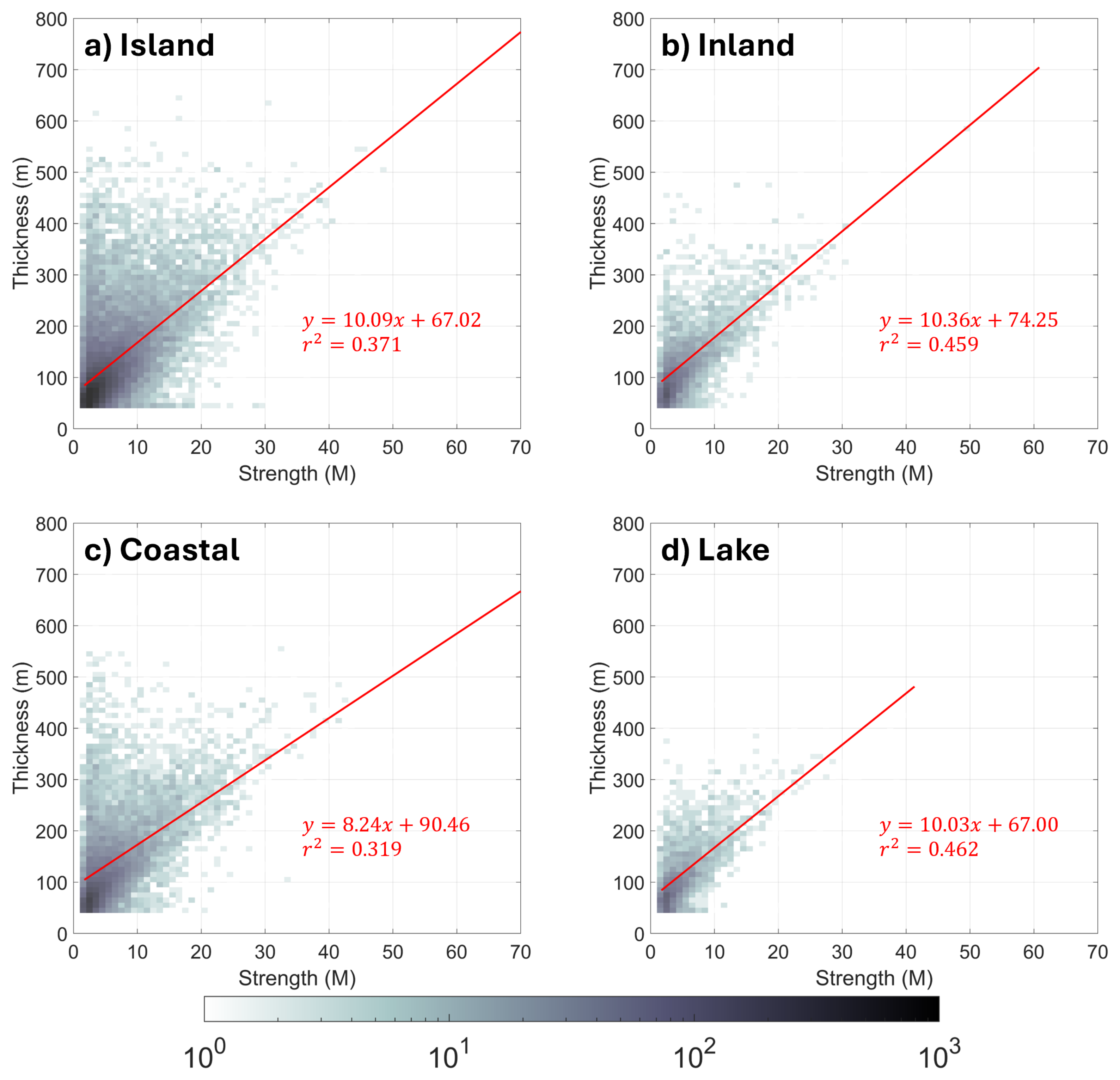
- Duct strength tended to increase with increasing duct thickness, but this relationship explained less than half of the variance.
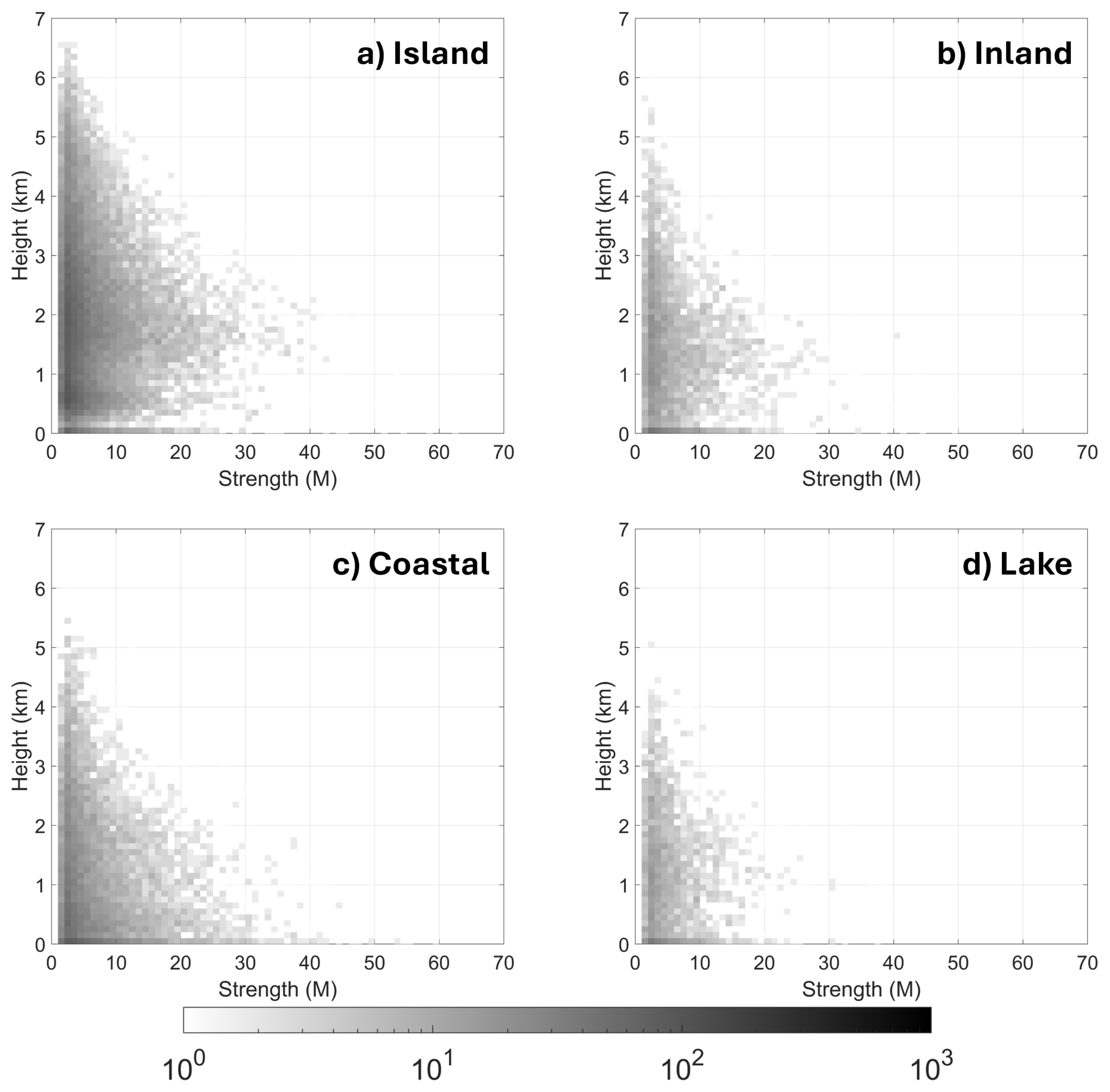
- The duct strength and duct base height were not correlated.
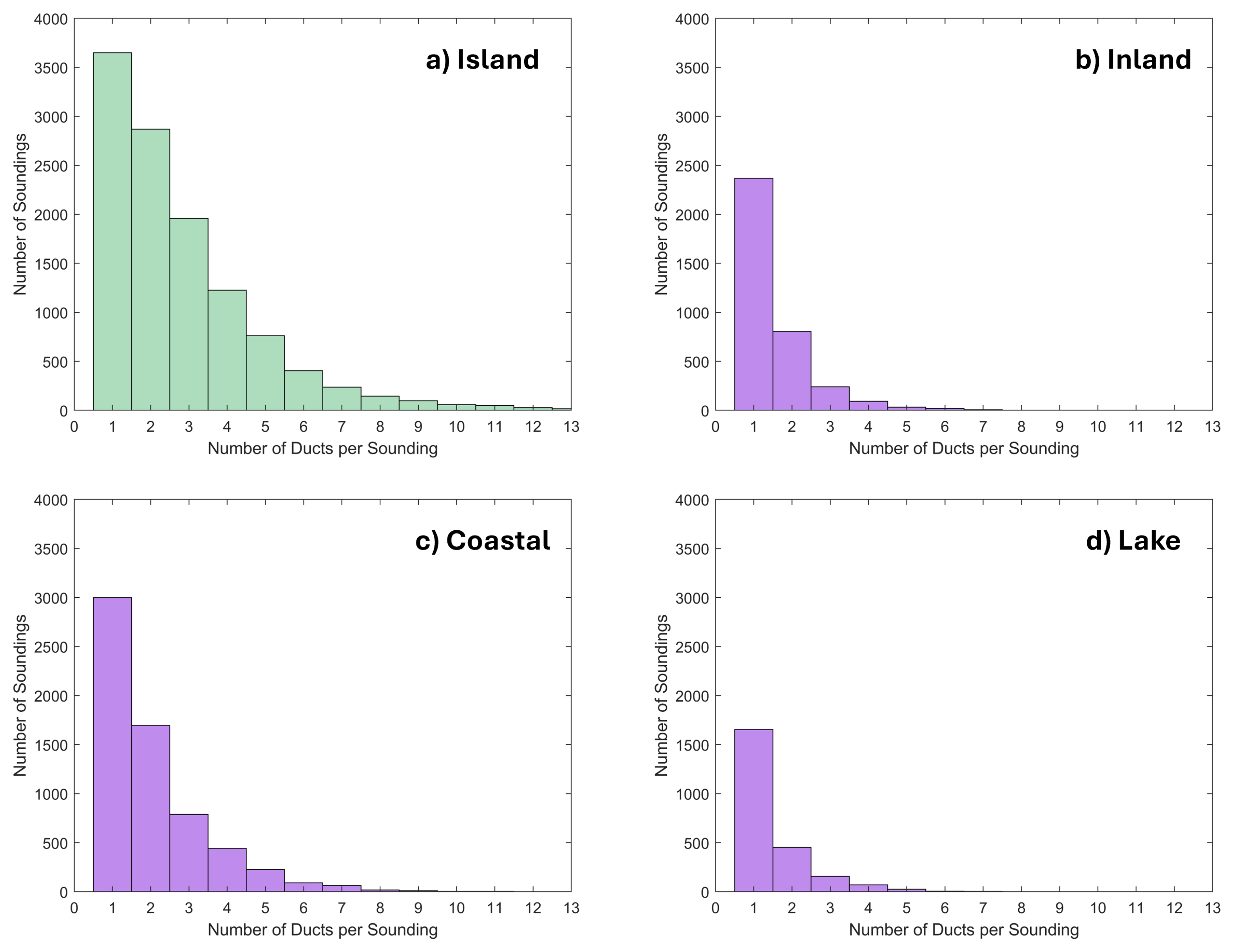
- Profiles with one or more ducts were common at the tropical and subtropical island (~60%) and US coastal locations (~70%), and they occurred less than 30% of the time at the Great Lakes and US inland sites.
- Notable differences between the ducts at tropical and subtropical islands versus the US coastal locations included islands that had higher median duct base altitudes, a higher frequency of stronger ducts at altitudes of > 1 km, and a lower frequency of surface-based ducts.
- The tropical and subtropical island locations often exhibited one or more elevated ducts above a 2 km altitude in a single profile—a phenomena requiring further investigation.
Author Contributions
Funding
Institutional Review Board Statement
Informed Consent Statement
Data Availability Statement
Acknowledgments
Conflicts of Interest
References
- Kerr, D.E. Propagation of Short Radio Waves, 1st ed.; Number 13 in Radiation Laboratory; McGraw-Hill Book Company Inc.: New York, NY, USA, 1951. [Google Scholar]
- Bean, B.R.; Dutton, E.J. Radio Meteorology; Dover Publications: Garden City, NY, USA, 1966. [Google Scholar]
- Rosenthal, J. Refractive Effects Guidebook; COMTHIRDFLT TACMEMO 280-1-76; Naval Ocean Systems Center: San Francisco, CA, USA, 1979; Available online: https://apps.dtic.mil/sti/tr/pdf/ADA034073.pdf (accessed on 16 December 2024).
- Kukushkin, A. Radio Wave Propagation in the Marine Boundary Layer; Wiley: New York, NY, USA, 2004. [Google Scholar]
- Cairns-McFeeters, E.L. Effects of Surface-Based Ducts on Electromagnetic Systems. Master’s Thesis, Naval Post Graduate School, Monterey, CA, USA, 1992. [Google Scholar]
- Turton, J.D.; Bennetts, D.A.; Farmer, S.F.G. An introduction to radio ducting. Meteorol. Mag. 1988, 117, 245–254. [Google Scholar]
- Saeger, J.T.; Grimes, N.G.; Rickard, H.E.; Hackett, E.E. Evaluation of simplified evaporation duct refractivity models for inversion problems. Radio Sci. 2015, 50, 1110–1130. [Google Scholar] [CrossRef]
- Thompson, W.T.; Haack, T. An Investigation of Sea Surface Temperature Influence on Microwave Refractivity: The Wallops-2000 Experiment. J. Appl. Meteorol. Climatol. 2011, 50, 2319–2337. [Google Scholar] [CrossRef]
- Alappattu, D.P.; Wang, Q.; Yamaguchi, R.T.; Haack, T.; Ulate, M.; Fernando, H.J.; Frederickson, P. Electromagnetic Ducting in the Near-Shore Marine Environment: Results From the CASPER-East Field Experiment. J. Geophys. Res. Atmos. 2022, 127, e2022JD037423. [Google Scholar] [CrossRef]
- Doyle, J.D.; Patel, R.N.; Reynolds, C.; Cobb, A. Impact of Atmospheric Rivers on Electromagnetic Ducting as Diagnosed from Dropsondes. J. Appl. Meteorol. Climatol. 2025. conditionally accepted. [Google Scholar]
- von Engeln, A.; Teixeira, J. A ducting climatology derived from the European Centre for Medium-Range Weather Forecasts global analysis fields. J. Geophys. Res. Atmos. 2004, 109, D18104. [Google Scholar] [CrossRef]
- ECMWF. European Center for Medium-Range Weather Forecasts (ECMWF) Model Level Definitions; ECMWF: Reading, UK, 2024; Available online: https://confluence.ecmwf.int/display/UDOC/Model+level+definitions (accessed on 16 December 2024).
- Cherrett, R.C. Capturing Characteristics of Atmospheric Refractivity Using Observations and Modeling Approaches. Ph.D. Thesis, Naval Postgraduate School, Monterey, CA, USA, 2015. [Google Scholar]
- Haack, T.; Wang, C.; Garrett, S.; Glazer, A.; Mailhot, J.; Marshall, R. Mesoscale Modeling of Boundary Layer Refractivity and Atmospheric Ducting. J. Appl. Meteorol. Climatol. 2010, 49, 2437–2457. [Google Scholar] [CrossRef]
- NCEI. Global BUFR Data Stream: Upper Air Reports from the National Weather Service Telecommunications Gateway (NWS TG); NCEI: Asheville, NC, USA, 2021. Available online: https://www.ncei.noaa.gov/access/metadata/landing-page/bin/iso?id=gov.noaa.ncdc:C01500;view=iso#idm140422537286768 (accessed on 16 December 2024).
- World Meteorological Organization. WIS Manuals; World Meteorological Organization: Geneva, Switzerland, 2022; Available online: https://community.wmo.int/activity-areas/wis/wis-manuals (accessed on 16 December 2024).
- Vaisala. Radiosonde RS41-SGE with BioCover; Vaisala: Vantaa, Finland, 2023; Available online: https://docs.vaisala.com/v/u/B212709EN-A/en-US (accessed on 16 December 2024).
- Brooks, I.M.; Goroch, A.K.; Rogers, D.P. Observations of Strong Surface Radar Ducts over the Persian Gulf. J. Appl. Meteorol. 1999, 38, 1293–1310. [Google Scholar] [CrossRef]
- Stull, R.B. An Introduction to Boundary Layer Meteorology; Springer: Dordrecht, The Netherlands, 1988. [Google Scholar]
- Parker, W.S. Model Evaluation: An Adequacy-for-Purpose View. Philos. Sci. 2020, 87, 457–477. [Google Scholar] [CrossRef]
- Alappattu, D.P.; Wang, Q.; Kalogiros, J. Anomalous propagation conditions over eastern Pacific Ocean derived from MAGIC data. Radio Sci. 2016, 51, 1142–1156. [Google Scholar] [CrossRef]
- Stevens, B. Atmospheric Moist Convection. Annu. Rev. Earth Planet. Sci. 2005, 33, 605–643. [Google Scholar] [CrossRef]
- de Szoeke, S.P.; Verlinden, K.L.; Yuter, S.E.; Mechem, D.B. The Time Scales of Variability of Marine Low Clouds. J. Clim. 2016, 29, 6463–6481. [Google Scholar] [CrossRef]
- Gerber, H.E.; Frick, G.M.; Jensen, J.B.; Hudson, J.G. Entrainment, Mixing, and Microphysics in Trade-Wind Cumulus. J. Meteorol. Soc. Jpn. Ser. II 2008, 86A, 87–106. [Google Scholar] [CrossRef]
- Riley, E.M.; Mapes, B.E.; Tulich, S.N. Clouds Associated with the Madden–Julian Oscillation: A New Perspective from CloudSat. J. Atmos. Sci. 2011, 68, 3032–3051. [Google Scholar] [CrossRef]


| Location Type | Total Soundings | # of Soundings with ≥1 Duct | Percent of Soundings with ≥1 Duct | Duct Count |
|---|---|---|---|---|
| Island | 19,524 | 11,538 | 59.1% | 32,352 |
| Coastal | 8850 | 6338 | 71.6% | 12,938 |
| Lake | 8871 | 2367 | 26.7% | 3508 |
| Inland | 11,992 | 3565 | 29.7% | 5403 |
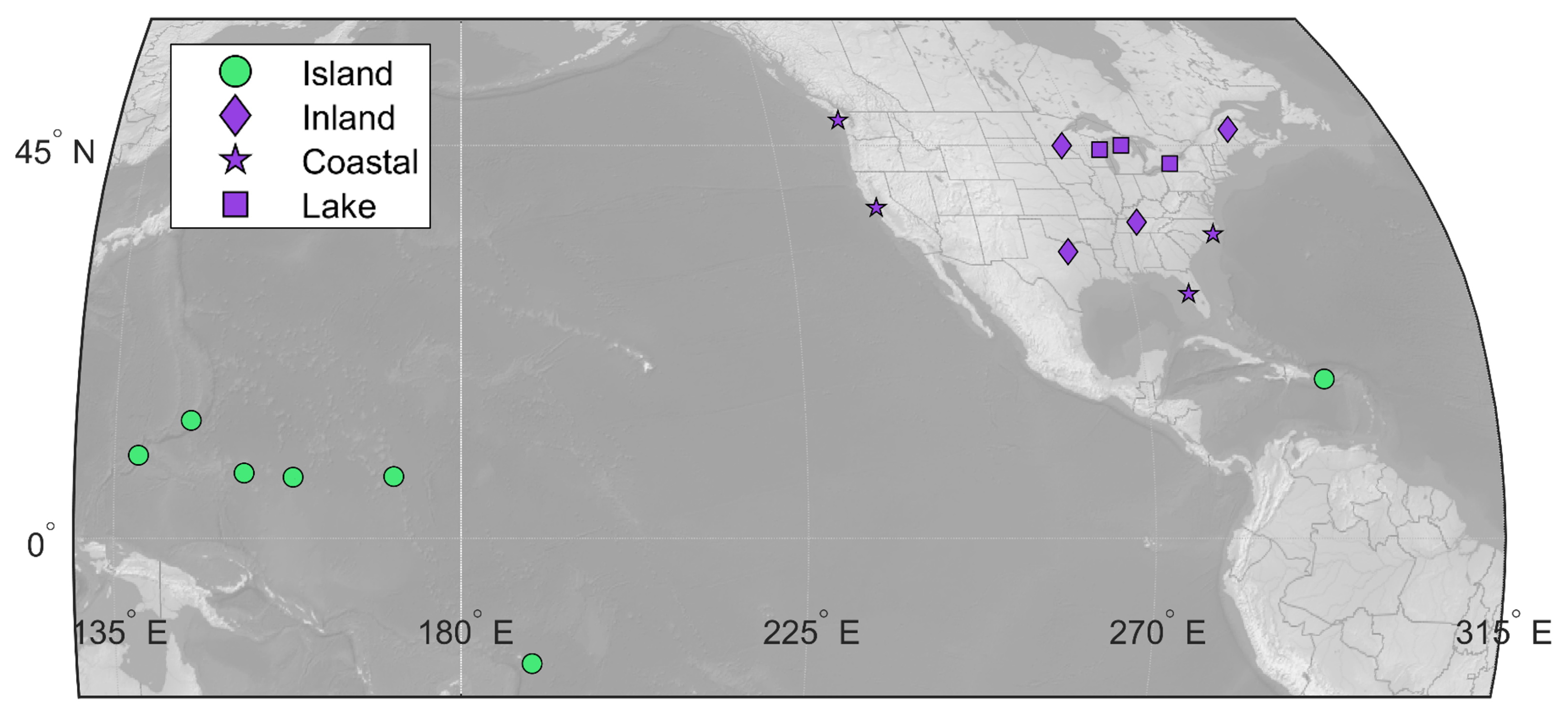
| Location Name | Latitude (°) | Longitude (°) | Local Time at 00 UTC | Local Time at 12 UTC |
|---|---|---|---|---|
| Island | ||||
| American Samoa | −14.33 | −170.71 | 1300 | 0100 |
| Chuuk | 7.46 | 151.84 | 1000 | 2200 |
| Guam | 13.48 | 144.80 | 1000 | 2200 |
| Marshall Islands | 7.06 | 171.27 | 1200 | 0000 |
| Micronesia | 6.99 | 158.21 | 1100 | 2300 |
| Puerto Rico | 18.22 | −66.59 | 2000 | 0800 |
| Yap | 9.50 | 138.08 | 1000 | 2200 |
| Coastal | ||||
| Oakland, CA | 37.80 | −122.27 | 1600/1700 | 0400/0500 |
| Newport, NC | 34.79 | −76.86 | 1900/2000 | 0700/0800 |
| Quilayute, WA | 47.94 | −124.54 | 1600/1700 | 0400/0500 |
| Tampa, FL | 27.95 | −82.46 | 1900/2000 | 0700/0800 |
| Lake | ||||
| Buffalo, NY | 42.89 | −78.88 | 1900/2000 | 0700/0800 |
| Gaylord, MI | 45.03 | −84.67 | 1900/2000 | 0700/0800 |
| Green Bay, WI | 44.51 | −88.01 | 1800/1900 | 0600/0700 |
| Inland | ||||
| Caribou, ME | 46.86 | −68.00 | 1900/2000 | 0700/0800 |
| Fort Worth, TX | 32.76 | −97.33 | 1800/1900 | 0600/0700 |
| Minneapolis, MN | 44.98 | −93.27 | 1800/1900 | 0600/0700 |
| Nashville, TN | 36.16 | −86.78 | 1800/1900 | 0600/0700 |
| 10th | 25th | Median | 75th | 90th | |
|---|---|---|---|---|---|
| Strength (M) | |||||
| Island | 2.04 | 2.66 | 4.13 | 7.23 | 12.40 |
| Coastal | 2.10 | 2.83 | 4.69 | 8.69 | 15.11 |
| Lake | 2.03 | 2.69 | 4.23 | 7.46 | 12.42 |
| Inland | 2.05 | 2.70 | 4.35 | 8.19 | 14.46 |
| Thickness (m) | |||||
| Island | 52 | 66 | 94 | 156 | 257 |
| Coastal | 55 | 73 | 114 | 191 | 298 |
| Lake | 54 | 72 | 104 | 164 | 238 |
| Inland | 58 | 76 | 113 | 179 | 276 |
| Duct Base Height (m) | |||||
| Island | 503 | 963 | 1781 | 2628 | 3589 |
| Coastal | 55 | 324 | 874 | 1730 | 2720 |
| Lake | 41 | 460 | 1128 | 1826 | 2599 |
| Inland | 83 | 649 | 1320 | 2060 | 2867 |
| Duct Top Height (m) | |||||
| Island | 627 | 1098 | 1935 | 2750 | 3689 |
| Coastal | 219 | 512 | 1018 | 1887 | 2720 |
| Lake | 177 | 579 | 1272 | 1969 | 2708 |
| Inland | 228 | 810 | 1490 | 2198 | 2975 |
| Criteria | Island | Coastal | Lake | Inland |
|---|---|---|---|---|
| Includes a surface-based duct | 281 (2.4%) | 631 (10.0%) | 283 (12.0%) | 393 (11.0%) |
| Includes ≥ 1 duct with base > surface and <2 km | 8724 (75.6%) | 5233 (82.6%) | 1829 (77.3%) | 2600 (72.9%) |
| Includes ≥ 3 ducts with base > surface and <2 km | 1475 (12.8%) | 1125 (17.8%) | 140 (5.9%) | 189 (5.3%) |
| Includes ≥ 1 duct ≥ 2 km altitude | 7051 (61.1%) | 1855 (29.3%) | 602 (25.4%) | 1120 (31.4%) |
| Includes ≥ 3 ducts ≥ 2 km altitude | 1637 (14.2%) | 132 (2.1%) | 25 (1.1%) | 51 (1.4%) |
Disclaimer/Publisher’s Note: The statements, opinions and data contained in all publications are solely those of the individual author(s) and contributor(s) and not of MDPI and/or the editor(s). MDPI and/or the editor(s) disclaim responsibility for any injury to people or property resulting from any ideas, methods, instructions or products referred to in the content. |
© 2025 by the authors. Licensee MDPI, Basel, Switzerland. This article is an open access article distributed under the terms and conditions of the Creative Commons Attribution (CC BY) license (https://creativecommons.org/licenses/by/4.0/).
Share and Cite
Yuter, S.E.; Sevier, M.M.; Burris, K.D.; Miller, M.A. Characteristics of Observed Electromagnetic Wave Ducts in Tropical, Subtropical, and Middle Latitude Locations. Atmosphere 2025, 16, 336. https://doi.org/10.3390/atmos16030336
Yuter SE, Sevier MM, Burris KD, Miller MA. Characteristics of Observed Electromagnetic Wave Ducts in Tropical, Subtropical, and Middle Latitude Locations. Atmosphere. 2025; 16(3):336. https://doi.org/10.3390/atmos16030336
Chicago/Turabian StyleYuter, Sandra E., McKenzie M. Sevier, Kevin D. Burris, and Matthew A. Miller. 2025. "Characteristics of Observed Electromagnetic Wave Ducts in Tropical, Subtropical, and Middle Latitude Locations" Atmosphere 16, no. 3: 336. https://doi.org/10.3390/atmos16030336
APA StyleYuter, S. E., Sevier, M. M., Burris, K. D., & Miller, M. A. (2025). Characteristics of Observed Electromagnetic Wave Ducts in Tropical, Subtropical, and Middle Latitude Locations. Atmosphere, 16(3), 336. https://doi.org/10.3390/atmos16030336