Article

Air Pollution Monitoring and Modeling: A Comparative Study of PM, NO2, and SO2 with Meteorological Correlations

by
Elżbieta Wójcik-Gront
* and
Dariusz Gozdowski
Department of Biometry, Institute of Agriculture, Warsaw University of Life Sciences, Nowoursynowska 159, 02-776 Warsaw, Poland
*
Author to whom correspondence should be addressed.
Atmosphere 2025, 16(10), 1199; https://doi.org/10.3390/atmos16101199
Submission received: 16 September 2025 / Revised: 10 October 2025 / Accepted: 15 October 2025 / Published: 17 October 2025
(This article belongs to the Section Air Quality)

Abstract

Monitoring air pollution remains a significant challenge for both environmental policy and public health, particularly in parts of Eastern Europe where industrial structures are undergoing transition. In this paper, we examine long-term air quality trends in Poland between 1990 and 2023, drawing on multiple sources: satellite observations (from 2019 to 2025), ground-based stations, and official national emission inventories. The analysis focused on sulfur dioxide (SO2), nitrogen dioxide (NO2), and particulate matter (PM10, PM2.5). Data were obtained from the Sentinel-5P TROPOMI sensor, processed through Google Earth Engine, and monitored by the Chief Inspectorate of Environmental Protection (GIOŚ, Warsaw, Poland) and the National Inventory Report (NIR, Warsaw, Poland), compiled by KOBiZE (The National Centre for Emissions Management, Warsaw, Poland). The results show a decline in emissions. SO2, for instance, dropped from about 2700 kilotons in 1990 to under 400 kilotons in 2023. Ground-based measurements matched well with inventory data (correlations around 0.75–0.85), but the agreement was noticeably weaker when satellite estimates were compared with surface monitoring. In addition to analyzing emission trends, this study examined the relationship between pollution levels and meteorological conditions across major Polish cities from 2019 to mid-2024. Pearson’s correlation analysis revealed strong negative correlations between temperature and pollutant concentrations, especially for SO2, reflecting the seasonal nature of pollution peaks during colder months. Wind speed exhibited ambiguous relationships, with daily data indicating a dilution effect (negative correlations), whereas monthly averages revealed positive associations, likely due to seasonal confounding. Higher humidity was consistently linked to higher pollution levels, and precipitation showed weak negative correlations, likely influenced by seasonal weather patterns rather than direct atmospheric processes. These findings suggest that combining different monitoring methods, despite their quirks and mismatches, provides a fuller picture of atmospheric pollution. They also point to a practical challenge. Further improvements will depend less on sweeping industrial reform and more on shifting everyday practices, like how homes are heated and how people move around cities.

1. Introduction

Air pollution is often described as one of the defining environmental challenges of the 21st century [1]. Its impacts cut across public health, ecosystems, and climate, yet the story is rarely straightforward [2,3]. Europe has made significant progress in reducing emissions through the adoption of cleaner technologies, stricter policies, and international frameworks, such as the Convention on Long-range Transboundary Air Pollution. However, tracking the actual changes in air quality remains challenging [4]. Emissions fluctuate across space and time, weather can distort short-term readings, and each monitoring method comes with its own blind spots [5]. Poland provides a particularly interesting case. Since 1990, the country has undergone significant economic and political changes, accompanied by dramatic shifts in its environmental profile. The modernization of energy infrastructure and industry has helped reduce some of the most obvious pollutants; however, the long-standing dependence on coal-fired power plants and solid fuels for home heating continues to weigh heavily [6]. Sulfur dioxide (SO2), nitrogen dioxide (NO2), and particulate matter remain the key culprits, and their persistence raises questions about the extent to which policy measures have effectively reshaped everyday practices [7]. Each monitoring tool sheds light on part of the problem but leaves something out. Ground-based stations give precise measurements at specific sites, but they are expensive and too sparse to capture regional variation [8]. Satellites, such as Sentinel-5P with its TROPOMI sensor, can scan the entire country and beyond; however, translating those column measurements into what people are actually breathing is not straightforward [9]. Emission inventories, on the other hand, are comprehensive in principle, covering sectors, fuels, and years, but they depend on assumptions and reporting practices that may smooth over local realities [10]. That said, combining these approaches offers a way forward. The spread of cloud-based platforms, such as Google Earth Engine, has made it easier to work across scales and datasets, thereby lowering the barrier to entry for large-scale geospatial analysis [11]. These tools have arrived just as air quality standards have tightened and public awareness of fine particulate matter and gaseous pollutants has grown. The timing is not accidental: better data both responds to and fuels political pressure.
In addition to integrating diverse monitoring approaches, recent efforts have also focused on understanding how pollution patterns relate to meteorological conditions. Temperature, wind speed, humidity, and precipitation all influence the transport, transformation, and accumulation of pollutants [12]. However, this relationship is complex. For example, winter months often show high pollution levels due to both increased heating demand and meteorological inversions [13], while summer brings more favorable dispersion conditions [14]. This highlights the importance of joint analysis of pollution and weather data, particularly at the city scale, where public exposure is greatest [15]. Against this backdrop, our study examines air pollution trends in Poland between 1990 and 2023 (and, in the case of satellite data, up to mid-2025), focusing on SO2, NO2, PM10, and PM2.5. We bring together satellite records, ground monitoring networks, emission inventories, and meteorological data with four primary aims: to trace long-term trends, to assess the consistency of different sources, to identify the primary drivers of change, and to evaluate the impact of meteorological conditions and the effectiveness of policies aimed at achieving cleaner air.
The approach is admittedly imperfect. No single method captures the full picture, but taken together, these sources can sketch a more grounded and realistic view of Poland’s changing atmosphere.

2. Materials and Methods

2.1. Main Emission Sources of SO2, NO2, PM10 and PM2.5 in Poland Based on NIR Data

National emission inventory data were drawn from the annual reports prepared by the National Centre for Emissions Management (KOBiZE, https://www.kobize.pl/, accessed on 15 September 2025). These National Inventory Reports (NIR, Warsaw, Poland) provide sector- and fuel-specific estimates of air pollutant emissions, compiled in accordance with the IPCC (Intergovernmental Panel on Climate Change, Geneva, Switzerland) guidelines and the EMEP/EEA (European Environment Agency, Kopenhagen, Denmark) methodology [16]. For this study, we used annual totals of SO2, NO2, PM10, and PM2.5 for the years 1990–2023. The inventories are constructed by combining activity data, such as fuel consumption, industrial production, or vehicle kilometers traveled, with emission factors derived from direct measurement campaigns and published values. Quality assurance and uncertainty analysis ensure consistency with international obligations, including the Convention on Long-range Transboundary Air Pollution and the EU National Emission Ceilings Directive [17]. While these procedures lend credibility to the inventories, it is essential to keep in mind that they inevitably rely on assumptions and generalized emission factors, which may not fully capture local variability. The primary drivers of SO2 emissions in Poland have long been fossil fuel combustion, particularly in public electricity and heat production, which is dominated by coal-fired power plants [18] (Table 1). Additional contributions come from residential heating, where solid fuels such as coal and wood remain common in household boilers, as well as from industrial processes in metallurgy and chemicals, and fuel refining. Over the past three decades, however, SO2 emissions have dropped sharply. The reasons include the introduction of flue gas desulfurization, the retirement of outdated plants, and a gradual, albeit uneven, shift away from coal [19,20]. NO2 emissions tell a somewhat different story. Road transport, particularly diesel-powered vehicles, remains the leading source, followed by power and heat generation, industrial combustion (such as cement plants, metalworks, and large boilers), and, to a lesser degree, household heating [21]. While emissions from energy and industry have declined through modernization and tighter regulation, transport remains stubborn, especially in cities where diesel traffic dominates. Particulate matter comes from both combustion and mechanical processes [22]. Household heating, particularly the use of low-efficiency stoves burning coal or wood, is the single largest source of PM10 and PM2.5. The industry also plays a role through cement production, metal processing, and chemical manufacturing. Transport contributes to pollution through both exhaust and so-called “non-exhaust” pathways, including brake wear, tire abrasion, and road dust resuspension. Agriculture introduces another layer, involving tilling, fertilization, and the release of ammonia-related secondary particles, whereas construction and demolition activities generate localized PM10 dust. In addition to these direct sources, secondary aerosols form through atmospheric chemical processes involving SO2, NOₓ, NH3, and volatile organic compounds, contributing significantly to PM2.5 concentrations. Seasonal variability in SO2, NO2, PM2.5, and PM10 in Central and Eastern Europe is typically U-shaped, with higher levels in winter (due to increased heating demand and reduced dispersion caused by inversions) and in summer (secondary aerosol formation under high solar radiation and humidity). This distribution has been reported in multiple studies across Europe and Asia [23,24,25] and is also characteristic of Poland [26], reflecting both changes in atmospheric self-purification capacity and varying loads on thermal power plants. Among these, PM2.5 is particularly concerning, given its ability to penetrate deeply into the lungs and bloodstream [27]. This highlights the dominant sources—residential burning and urban transport—as critical priorities for air quality policy.

2.2. Ground-Based Monitoring Data

Ground-level air quality measurements were obtained from the national monitoring network operated by the Chief Inspectorate of Environmental Protection (GIOŚ, https://powietrze.gios.gov.pl/pjp/archives, accessed on 15 September 2025). The meteorological data were obtained from the Institute of Meteorology and Water Management (IMGW, https://danepubliczne.imgw.pl, accessed on 15 September 2025). This network comprises approximately 150 automatic monitoring stations distributed across Poland, measuring concentrations of major air pollutants including PM10, PM2.5, NO2, and SO2. Data were collected for the period of 2000–2023, providing a 24-year time series of annual average concentrations. Quality assurance procedures included validation of measurement techniques according to European standards (EN 14211 for NO2, EN 14212 for SO2, EN 12341 for PM10, and EN 14907 for PM2.5, https://standards.iteh.ai/catalog/standards/cen, accessed on 15 September 2025), regular calibration protocols, and statistical outlier detection [28]. To ensure data representativeness and consistency across years, we applied a threshold of at least 10 valid annual measurements from monitoring stations nationwide for each pollutant. Years with fewer than 10 available measurements were excluded from the analysis. This criterion particularly affected the early stage of PM2.5 monitoring, when the measurement network was still under development and data coverage was insufficient. For correlation analysis between ground-based pollutant data and meteorological variables, we used measurements from 17 automatic monitoring stations located in major Polish cities: Białystok, Gdańsk, Gorzów Wielkopolski, Katowice, Kielce, Kraków, Lublin, Łódź, Olsztyn, Opole, Poznań, Rzeszów, Szczecin, Toruń, Warsaw, Wrocław, and Zielona Góra. According to the official GIOŚ classification, these stations are predominantly urban background sites, designed to represent population exposure to ambient air pollution under typical urban conditions, rather than being influenced directly by local traffic or industrial sources. This ensures that the data reflect general trends in urban air quality over time.
This study analyzed correlations between air pollutants and meteorological variables in major Polish cities from January 2019 to June 2024. For each city, data from at least one monitoring station were used, and missing values were handled by pairing only available observations. Pearson correlation coefficients were calculated to assess relationships between pollutants and meteorological variables using both daily and monthly averaged data. All data were standardized prior to analysis to allow for comparison across variables and cities. The analyses were conducted using Python 3.12 (in Colab environment) libraries, including pandas for data handling, NumPy for numerical operations, Matplotlib 3.10.0 and Seaborn 0.13.2 for visualization, statsmodels 0.14.5, and scikit-learn 1.6.1 for trend estimation and data standardization. Exploratory data analyses were performed using scatter plot matrices with LOWESS smoothing, Theil–Sen trend estimation on monthly averages, and quarterly standardized heatmaps to visualize temporal patterns and relationships among variables.

2.3. Satellite-Based Data Collection for NO2 and SO2 Using Google Earth Engine

Tropospheric concentrations of NO2 and SO2 were retrieved from satellite observations via the Google Earth Engine (GEE) platform. Unlike these gases, particulate matter is not directly retrieved from TROPOMI, as the instrument measures aerosol optical depth rather than ground-level PM concentrations. This requires additional modeling and calibration, which introduces considerable uncertainty. Therefore, the PM data in this study were based solely on ground-based monitoring stations. GEE, a cloud-based geospatial analysis system developed by Google, provides researchers with access to vast satellite archives, along with the computing power needed for large-scale environmental studies [29]. For this work, we relied primarily on data from the Sentinel-5P mission, specifically the TROPOMI (Tropospheric Monitoring Instrument) sensor (European Space Agency, Paris, France). Sentinel-5P, part of the Copernicus programme led by the European Space Agency (ESA, Paris, France), was designed to monitor atmospheric trace gases with both high spatial and temporal detail. The datasets used here provide gridded (Level-3) information on tropospheric column concentrations, expressed in mol·m–2. These values are pre-processed and aggregated into daily means on a regular latitude-longitude grid, with a resolution of about 3.5 × 7 km2 at nadir. Our analysis spanned a continuous six-year period, from 1 April 2019, to 1 July 2025, which we divided into quarterly intervals corresponding to the meteorological seasons. This choice was not arbitrary: quarterly means balancing the need to capture broad seasonal cycles with the practical advantage of reducing “noise” from short-lived events, such as a winter smog episode or a single wind-driven transport plume that would otherwise dominate shorter time averages. Since satellite products report values in mol·m–2, we also converted them to μg·m−3 to allow for comparison with ground-based measurements. This conversion is inherently approximate and rests on assumptions about atmospheric conditions such as boundary layer height, pressure, and temperature. It is also worth underlining the caveats of satellite-based monitoring [30]. Cloud cover can mask retrievals; vertical columns do not perfectly reflect surface-level concentrations; once-daily overpasses miss much of the diurnal cycle; and occasional data gaps appear due to sensor or orbital constraints. Despite these issues, the GEE framework proved highly useful. It allowed reproducible access to consistent long–term datasets and made it feasible to assess spatial and seasonal patterns of pollution at the scale of an entire country.

3. Results

3.1. Long-Term NIR Data Analysis

Figure 1 illustrates the changes in national emissions of four major air pollutants in Poland between 1990 and 2023, as reported in the NIR. The most dramatic change is seen in SO2, which fell from more than 2700 kt in 1990 to under 400 kt in 2023. NO2 also declined, though more steadily, from roughly 1100 kt in 1990 to about 500 kt in 2023. PM10 fell from around 750 kt to roughly 300 kt, while PM2.5 dropped from about 400 kt to just over 200 kt. These reductions are linked to upgrades in household heating systems, stricter emission standards in transport, and modernization across industry. Nevertheless, over the last decade, the two curves have drawn closer together, indicating the persistent influence of fine particulates, primarily from domestic coal and wood burning, as well as traffic-related sources. Taken together, the figure highlights both the scale of progress and the limits of current measures. Poland has clearly benefited from decades of environmental regulation and technological advancements; yet, the persistence of particulate emissions indicates that some of the most significant challenges lie not in large-scale industry, but in everyday energy use and mobility. The trends also set the stage for comparing inventory-based estimates with satellite retrievals and modeled concentrations in the following sections.

3.2. Ground-Level Concentration Trends (2000–2023)

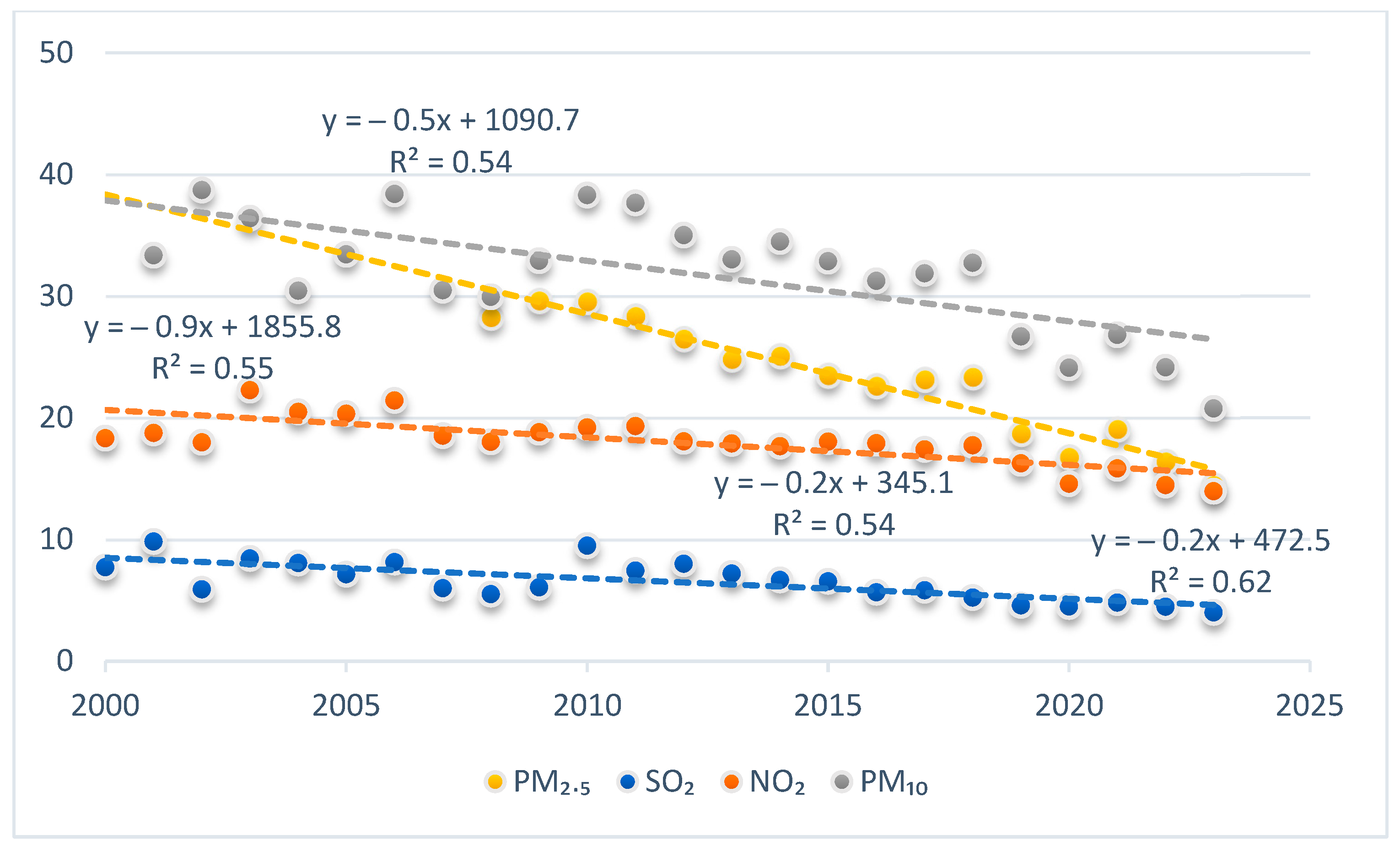
Among the pollutants analyzed from ground-level monitoring stations in Poland between 2000 and 2023 (Figure 2), PM10 consistently recorded the highest concentrations. While year-to-year variability is substantial, the overall trajectory points downward, with a more noticeable decline after 2018. PM2.5, which was first measured in 2004 but only in a few places (not shown in the figure), exhibited elevated levels in its early years, peaking around 2009. Since about 2011, concentrations have gradually decreased, though not always smoothly. NO2 levels remained relatively stable until approximately 2010, after which a modest decline became visible, becoming more pronounced after 2020. SO2 concentrations, by contrast, were much lower throughout the entire record and show a steady, unmistakable downward trend. Taken together, these patterns reflect national and EU-wide efforts to clean the air, including stricter emission standards, improved fuel quality, and the modernization of heating systems. Nevertheless, the persistence of relatively high PM10 and PM2.5 in earlier years, and their stubborn presence during winter months even more recently, points to the ongoing influence of household stoves and small-scale combustion. These are diffuse, local sources that regulations struggle to tackle as effectively as large industrial emitters. The ground-based monitoring dataset presented here, therefore, serves not just as a benchmark for comparing with satellite and modeled data in the following sections, but also as a reminder that progress at the national level may mask persistent, seasonal, and very local pollution problems.

3.3. Satellite-Derived Concentrations of NO2 and SO2 (2019–2025)

Figure 3 shows the temporal evolution of satellite-derived atmospheric concentrations of NO2 and SO2 in Poland between the second quarter of 2019 and the second quarter of 2025. NO2 concentrations remain relatively stable over time, generally fluctuating between 3.5 and 4.5 µg·m–3. A modest seasonal cycle is visible, with slightly higher values during first-quarter periods (winter months), which may be linked to residential heating and increased traffic demand. Unlike NO2, SO2 shows pronounced seasonal swings. Concentrations peak consistently in the fourth quarter, often reaching 50–65 µg·m–3, coinciding with winter heating demand. In contrast, summer values frequently drop into single digits, reflecting reduced fuel combustion outside the heating season. Seasonal effects predominate in the dataset, and no discernible downward trend is evident over the six years. The persistence of wintertime spikes suggests that high-sulfur fuels are still used in specific sectors or regions, despite broader reductions in coal dependence. The apparent seasonality of SO2 reflects its strong association with heating-related emissions and winter meteorological conditions, such as temperature inversions. By contrast, the steadier NO2 profile likely reflects more continuous sources, such as road transport and industrial combustion. Although limited in their ability to precisely capture surface concentrations, these satellite-derived estimates complement ground-based and inventory datasets by offering a consistent, large-scale perspective on temporal dynamics in pollutant levels.

3.4. Correlation Analysis Between Ground-Based, Inventory, and Satellite-Derived Pollutant Data

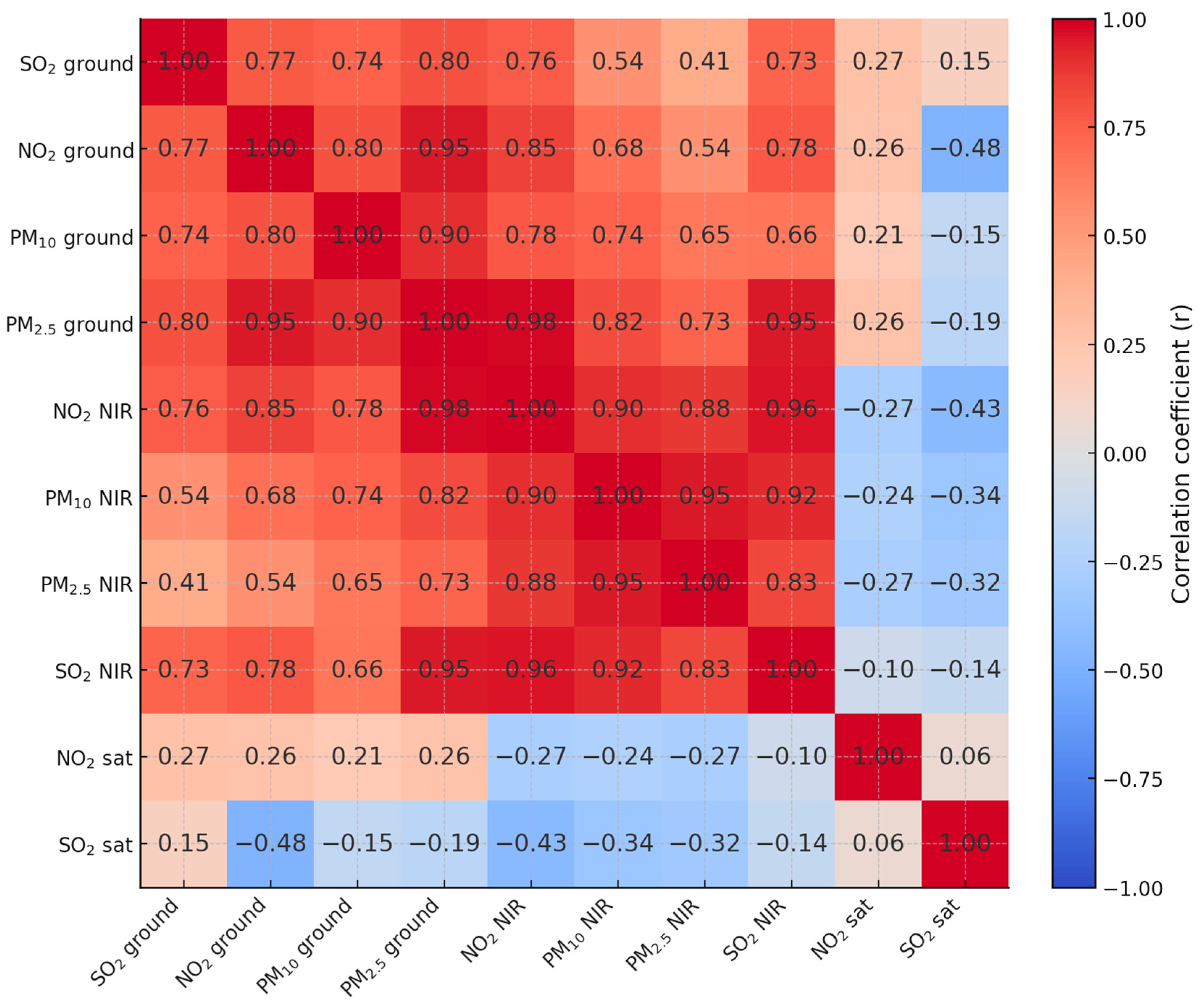
Figure 4 shows the Pearson correlation coefficients between different datasets for SO2, NO2, PM10, and PM2.5. The comparison draws on three sources: ground-based monitoring, national emission inventories, and satellite-derived estimates from Sentinel-5P processed in Google Earth Engine. For correlation analysis, datasets were harmonized by year, and missing values were excluded pairwise. The number of valid pairs varied between data sources: 16–24 for ground-based measurements, 34 for NIR data, and 7 for satellite data. The number of overlapping pairs between datasets ranged from 5 to 24, depending on the pollutant. Ground observations and NIR data align well, with strong correlations observed for NO2 (r = 0.85), PM10 (r = 0.74), and SO2 (r = 0.73). This suggests that inventory-based emission trends capture real atmospheric concentrations reasonably well, at least for pollutants closely tied to combustion processes such as traffic, residential heating, and energy production. Correlations within the NIR dataset itself are even higher (NO2–SO2: 0.96, PM10–PM2.5: 0.95, NO2–PM2.5: 0.88), reflecting the shared role of fossil fuel use across sectors. The picture appears different when satellite products are taken into account. For NO2, the correlation between tropospheric column retrievals and ground-level concentrations is modest (0.26), hinting that vertical distribution and meteorological influences complicate the link between what satellites “see” and what people breathe. For SO2, the situation is even more challenging: correlations with ground data are very low or even negative (SO2_sat–SO2_ground: 0.15; SO2_sat–NO2_ground: −0.48). Similarly, comparisons between satellite retrievals and NIR data show weak or negative associations (NO2_sat—NO2_NIR: −0.27; SO2_sat—SO2_NIR: −0.14). These mismatches are not surprising, given that satellite products represent atmospheric columns. At the same time, inventories are based on bottom-up sectoral activity data aggregated annually, and the variable number of valid data pairs across the different datasets. Interestingly, correlations between different pollutants at ground stations are also notable: PM10 and NO2 (0.80), PM2.5 and PM10 (0.90), and SO2 and NO2 (0.77)—again underscoring common emission sources such as road transport, household heating, and specific industries. Taken together, the results highlight both the value and the limits of each approach. Inventories appear to track real-world concentrations reasonably well, while satellites provide crucial spatial coverage but struggle to represent surface conditions for certain pollutants, particularly SO2, accurately.

3.5. Correlation Analysis Between Ground-Based Pollutant Data and Meteorological Variables

For the correlation analysis between ground-based pollutant data and meteorological variables data derived from the main cities of Poland, data were used for the period from the beginning of 2019 to the end of the first half of 2024. The cities included in the analysis were as follows: Białystok, Gdańsk, Gorzów Wielkopolski, Katowice, Kielce, Kraków, Lublin, Łódź, Olsztyn, Opole, Poznań, Rzeszów, Szczecin, Toruń, Warsaw, Wrocław, and Zielona Góra. The pollution data were obtained from the monitoring stations of GIOŚ. For each city, data from at least one monitoring station measuring pollution levels were used. The pollutants considered were PM2.5, PM10, NO2, and SO2. The meteorological data also originated from the same cities and were obtained from IMGW. Since both the air pollution data and the meteorological data were not fully complete due to missing measurements, the correlations were calculated by pairing the available data. Table 2 presents the basic statistics of the variables used for the analyses across all cities from January 2019 to June 2024. The results indicate that most of the variables have slightly higher means than medians, which indicates their right-skewed distribution. The variability in all four pollutants, expressed as the coefficient of variation, was quite large and similar for all pollutants. The most stable meteorological variables were air pressure and air humidity, but the highest variability was observed for precipitation.
Figure 5 shows the standardized monthly averages of selected environmental variables (PM2.5, SO2, wind speed, and temperature) from January 2019 to June 2024, with the seasons of the year clearly marked. The highest level of pollution was observed during winter, especially during the coldest months, i.e., January and February, during the peak of heating season, when many households heat their homes with coal and other types of fuel that cause significant emissions of PM and SO2. The pollution level was opposite to the temperature pattern; i.e., the lowest pollution levels were observed during summer, especially in July and August, when emissions related to home heating are not present. The highest wind speeds in Poland are typically observed during winter, resulting in a similar pattern of wind speeds to the pattern of pollution levels. Since the chart presents monthly averages, daily fluctuations are not visible, although they are important when analyzing the relationship between pollution levels and wind speed. The results shown in Figure 6 confirm a positive association between pollution levels for the averaged monthly data. However, this is a spurious correlation resulting from the fact that higher wind speeds are observed in months with lower temperatures. In contrast, for daily data, the relationship is negative (correlation coefficients below 0), which is because pollution levels in cities (as the measurement stations were located only in urban areas with higher population density) are lower during periods of stronger winds, since air pollutants are dispersed in the atmosphere outside the cities.
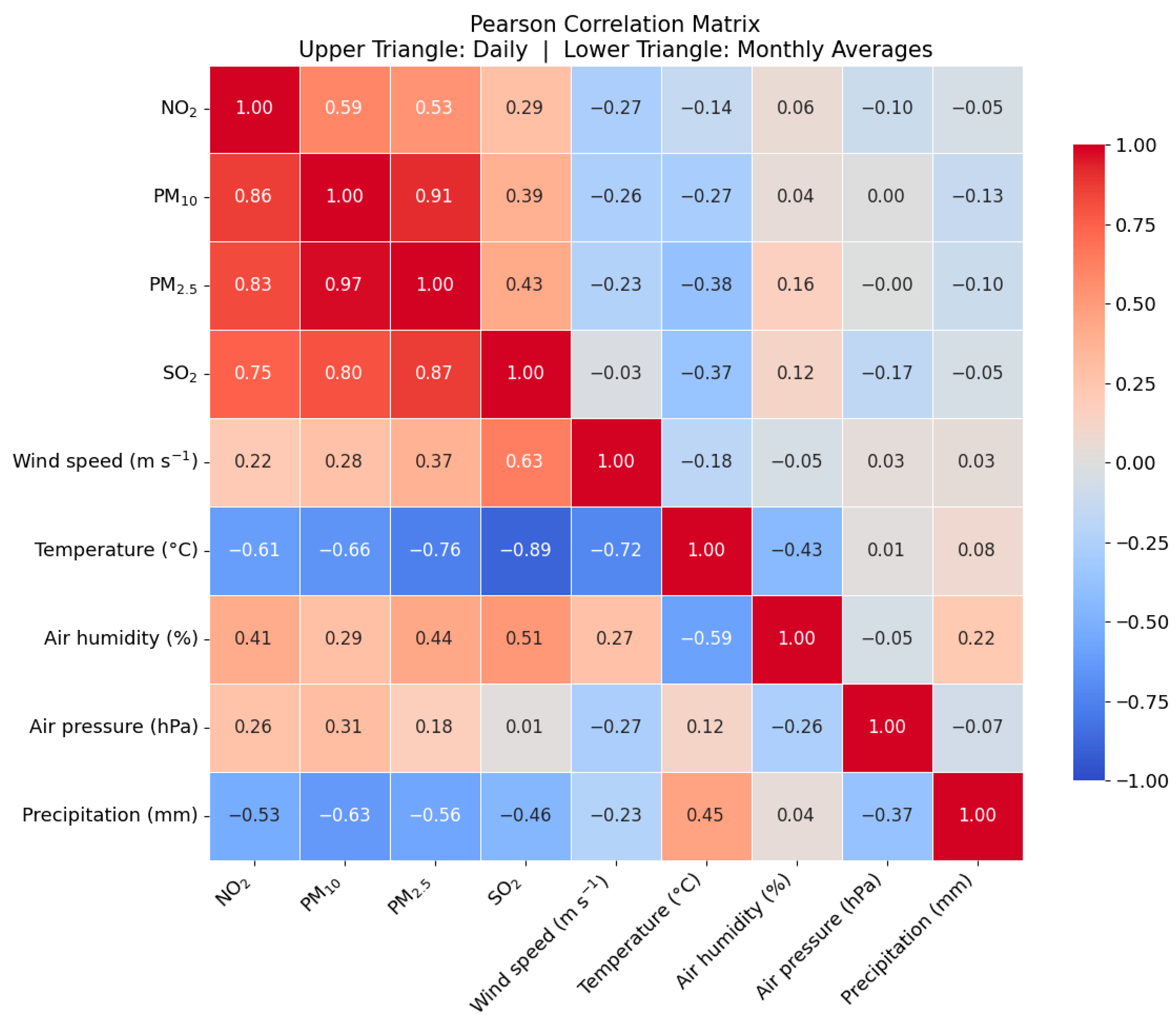
Figure 6 presents the Pearson correlation coefficients between selected environmental variables for the period from January 2019 to June 2024 as a heatmap. The upper triangle displays correlations based on daily data, while the lower triangle shows correlations based on monthly averages. The correlations based on monthly averages were stronger for all variables. The strongest positive correlations were observed between various pollutants, especially between PM10 and PM2.5. The strongest correlations between pollution levels and meteorological variables were observed for temperature, which was negatively correlated with all pollutants, especially with SO2. Ambiguous correlations were observed between wind speed and all pollutants. For correlations based on monthly averaged data, positive relationships were observed, whereas for daily data, negative correlations were found. This can be explained by the fact that the positive correlations in the averaged data are rather spurious, resulting from generally higher pollution levels during the winter season. In the case of daily data, the correlation is weaker but negative, most likely because higher wind speeds contribute to faster dispersion of pollutants in the atmosphere, leading to lower concentrations within urban areas. In the case of air humidity, correlations with all pollutants were positive, indicating that higher pollution levels are observed during humid conditions. Precipitation was correlated negatively with pollution levels; however, this correlation is likely spurious, due to generally lower pollution levels during the summer season, when higher precipitation is observed.
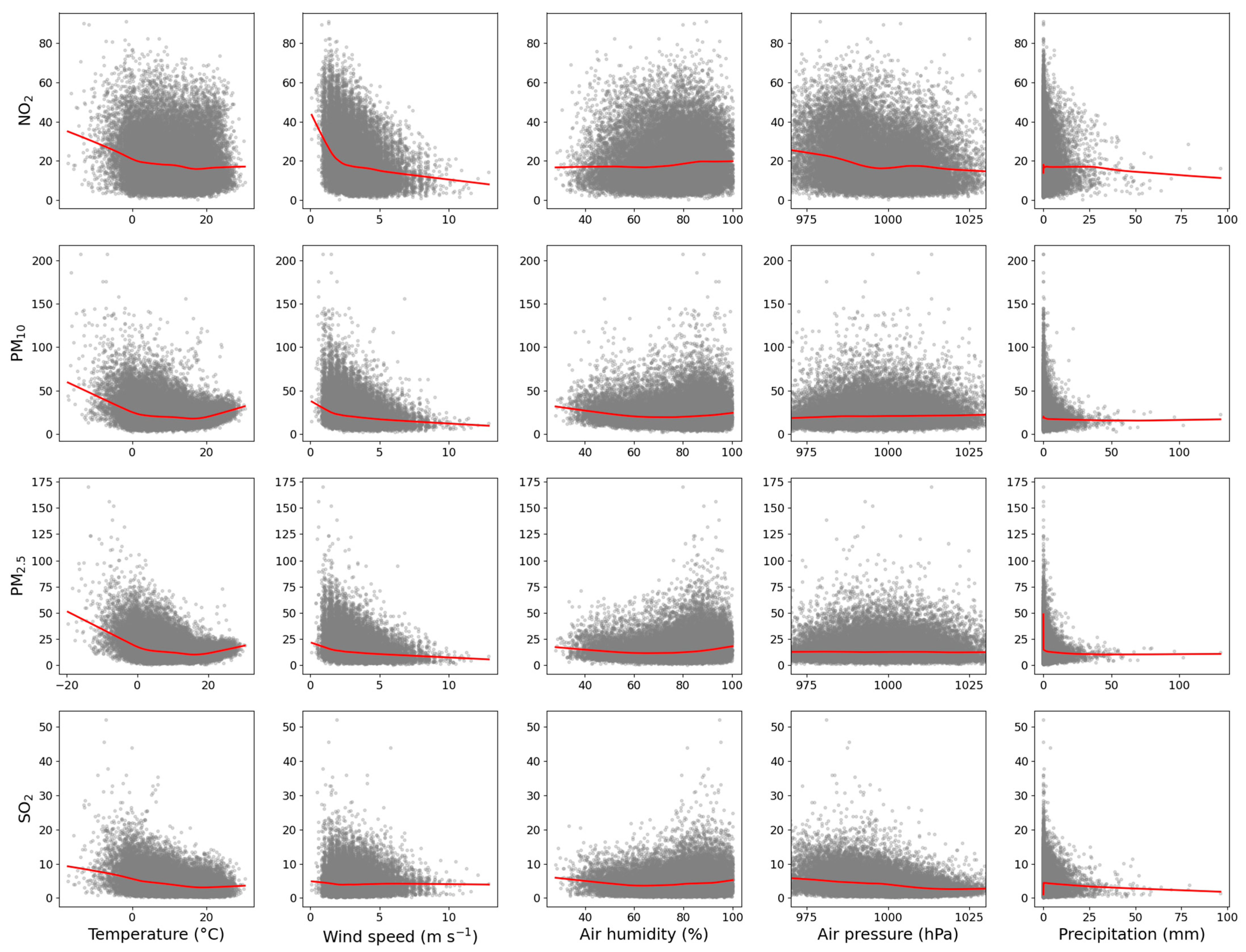
To evaluate the patterns of relationships between pairs of variables, a scatter plot matrix (Figure 7) was prepared between variables which characterize weather conditions (temperature, wind speed, humidity, air pressure, and precipitation) with variables which characterize pollution level (PM2.5, PM10, NO2, SO2). Scatter plots for each pair of variables were overlaid with locally weighted LOWESS smoothing lines to highlight trends. This visualization proved near-linear relationships between most of the variables. The only clearly non-linear relationships observed were between wind speed and the content of NO2 in the atmosphere. An increase in wind speed from 0 to about 3 m s−1 resulted in a nearly 2-fold decrease in NO2, and further increases in wind speed caused only a very small decrease in this pollutant. A similar pattern is observed between temperature and the content of PM10 and PM2.5. A large decrease is observed with an increase in temperature from about −15 °C to about 0 °C but a further increase in temperature above 0 °C no longer leads to additional reductions in PM, and at very high temperatures above 25 °C, a slight increase in PM is even observed. The relationships between weather variables and air pollutants are not very strong, partly because both the pollutant concentrations and the meteorological variables exhibit high temporal variability.
Figure 8 presents line plots of monthly averaged air pollution and meteorological variables with linear regression trend lines, showing linear trends over time and calculating annualized slopes for each variable. The patterns indicate very strong seasonal variability in all variables. The linear regression trend analysis of monthly averaged data from 2019 to mid-2024 indicates a general decrease in air pollutant concentrations, with annual declines of −0.860 µg·m−3 for NO2, −1.234 µg·m−3 for PM10, −0.71 µg·m−3 for PM2.5, and −0.23 µg·m−3 for SO2. In contrast, meteorological variables exhibit smaller changes, including a rise in temperature of 0.14 °C per year and slight increases in air humidity and precipitation, while wind speed and air pressure show minor decreases.
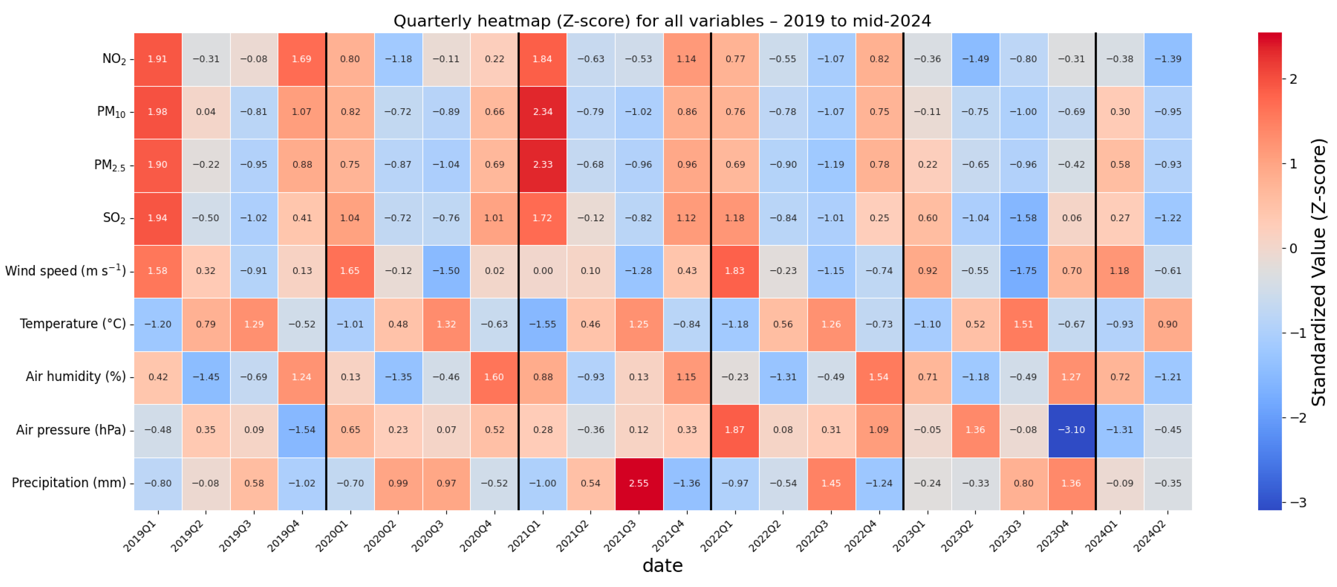
Figure 9 presents a quarterly heatmap of all selected air pollution and meteorological variables, with values standardized as Z-scores. The resulting visualization highlights seasonal and interannual patterns, showing that pollutant concentrations (NO2, PM10, PM2.5, SO2) are generally higher in winter quarters and lower in summer, while temperature, wind speed, and other meteorological variables exhibit expected seasonal cycles. Standardization enables direct comparison across variables, highlighting periods with unusually high or low values relative to their typical range.

4. Discussion

The sharp decline in emissions over the study period, most strikingly the drop in SO2, points to the impact of wide-ranging environmental policies adopted in Poland since the early 1990s [31]. Two EU directives in particular, the Large Combustion Plant Directive (2001/80/EC) and its successor, the Industrial Emissions Directive (2010/75/EU), played a central role in pushing the power and industrial sectors toward cleaner technologies. Flue gas desulfurization systems became standard, and older, inefficient plants were gradually phased out, both of which substantially reduced SO2 emissions [32]. NO2 reductions have been less dramatic but still noticeable. Here, the incremental tightening of vehicle emission standards (from Euro 1 to Euro 6) helped offset the growth in traffic volumes and vehicle fleets [33]. The EU Emission Trading System (EU ETS) has also provided additional incentives for cutting emissions at large stationary sources, offering a market-based complement to regulatory pressure [34]. Particulate matter, however, has proven harder to tame. PM2.5 levels, in particular, remain stubbornly elevated, largely because their sources, small-scale residential heating with coal and wood, are diffuse and deeply tied to household practices [35]. Measures such as low-emission zones in major cities and national programs for replacing outdated stoves are important steps. Nevertheless, the slow pace of change highlights the challenges of regulating these sources compared to industrial smokestacks or power plants. The comparison of satellite, ground-based, and inventory datasets adds another layer of insight. Strong correlations between ground monitoring and the NIR inventory (r = 0.76 to 0.85) suggest that Poland’s reporting system is broadly reliable and that the emission factor-based inventory approach captures real trends reasonably well. But the weaker, sometimes even negative, correlations with satellite retrievals remind us of the methodological gap between the two. A limitation of our correlation analysis is the variable number of valid data pairs across the different datasets. While ground-based monitoring and NIR data provided sufficient temporal coverage, the satellite dataset was available only for a shorter period. However, correlations based on a small number of pairs, particularly those derived from satellite data, should be interpreted with caution. This limitation reflects the relatively recent availability of satellite observations (since 2019) rather than a methodological issue. It highlights the importance of integrating long-term ground-based measurements with emerging remote sensing products. Satellites measure column-integrated concentrations, which depend heavily on vertical profiles, boundary layer dynamics, and weather [36]. Any attempt to convert those values into near-surface concentrations requires assumptions that may or may not hold, especially for gases with steep vertical gradients. In addition to that, timing matters: Sentinel-5P passes over at about 13:30 local time, while ground stations report 24 h averages. Diurnal cycles in emissions and atmospheric chemistry can create substantial differences between the two perspectives, making direct comparisons far from straightforward. The role of meteorological factors in shaping pollution levels further complicates the interpretation of air quality trends. Our analysis across 17 major Polish cities between 2019 and mid-2024 shows clear seasonal patterns in pollutant concentrations, with winter months consistently recording the highest levels of SO2 and PM2.5. These peaks coincide with increased heating demand and atmospheric conditions, such as temperature inversions, which hinder pollutant dispersion. The obtained results are consistent with those of other studies on air pollution in urban or industrial environments [37,38,39]. Typical correlations between temperature and SO2 and PM air pollution are negative if the data are studied across the year. However, evaluating these correlations separately for each season (spring, summer, autumn, and winter) yields ambiguous results. In the study conducted by Eren et al. [39] in Turkey, the correlation between temperature and PM10 was negative only for autumn; however, for other seasons, especially summer, the correlations were positive. Evaluation of correlations between pollutants and meteorological elements at various temporal scales, such as monthly, daily, and hourly scales, can yield different results [40]. Therefore, it is crucial to evaluate the correlation at an appropriate temporal scale, depending on the analysis’s aim. Some studies do not contain information about the temporal scale at which the correlations were evaluated, which may lead to a misinterpretation of the results. The strong negative correlation between temperature and pollutant levels, particularly SO2, confirms the winter-related nature of these emissions. However, correlations with other meteorological variables such as wind speed and humidity are more ambiguous. The analyses indicate that relationships between air pollutants and meteorological variables are linear and generally moderate, with some clearly nonlinear patterns, such as the effects of wind speed on NO2 and temperature on particulate matter, suggesting threshold behaviors in pollutant dispersion and accumulation. Seasonal variability has a strong influence on all variables, with pollutant concentrations peaking in winter and decreasing in summer, while meteorological conditions follow the expected seasonal cycles. We must also be aware of various other types of fluctuations in air pollution levels, such as those that depend on the time of day and those that depend on the day of the week. Typically, slightly higher levels of PM, NO2, and SO2 are observed during the day compared to nighttime, and on weekdays compared to weekends [38,41,42]. Long-term trends show a gradual decline in air pollutant levels, particularly NO2 and PM10, whereas changes in meteorological variables are relatively minor. Overall, these results suggest that both meteorological factors and emission patterns influence air quality; however, high temporal variability and nonlinear interactions limit the strength of direct correlations. Wind speed shows negative correlations with pollution on a daily scale (consistent with its dispersive effect), but weakly positive correlations on a monthly scale, likely due to seasonal confounding, stronger winds, and higher emissions, both of which occur during winter [43]. Similarly, higher humidity correlates positively with pollutant concentrations, possibly reflecting stagnant and moist air conditions typical of smog episodes. However, in a coastal city in India, higher humidity appears to help remove particulates from the air, likely due to wet deposition and particle agglomeration, rather than increasing pollution levels [44]. This may reflect regional or seasonal differences, or possibly the role of humidity-related atmospheric stagnation in some inland or urban settings. Precipitation shows weak negative associations, again influenced by seasonal patterns rather than direct causality [45]. These findings underscore the importance of considering weather conditions when interpreting air quality data or evaluating the effectiveness of policies. Without considering meteorology, temporary improvements (e.g., due to a mild winter or strong winds) may be mistakenly attributed to regulatory success, while pollution spikes tied to seasonal factors could obscure long-term progress. This reinforces the value of combining high-frequency meteorological data with pollutant measurements to distinguish structural changes from short-term variability. Moreover, the observed relationships between pollutants and weather further emphasize the limits of technical or regulatory fixes alone. Cleaner technologies and emission standards are necessary but insufficient when diffuse, weather-dependent sources, such as household heating, dominate winter air quality. Policy instruments must therefore be complemented by behavioral, infrastructural, and social interventions, including public awareness campaigns, subsidies for clean heating systems, and local air quality alerts timed to meteorological conditions. As our analysis shows, progress in air quality now depends as much on changing everyday practices as it does on controlling industrial emissions.
It is worth noting that similar correlations exist between various meteorological variables and the levels of PM, SO2, and NO2 pollution in regions where home heating is required, often involving the use of coal or other fuels. In regions with warm or tropical climates, these relationships may be entirely different. An example is the study by Sharma et al. [46], conducted in a semi-arid environment, which found a positive relationship between temperature and PM10, while no strong correlations were observed with SO2 and NO2. Similar results were observed in the study of Morshed et al. [47] conducted in Bangladesh in a tropical climate. A positive correlation was found between temperature and air pollution, specifically in terms of NO2 and SO2 levels. The relationships between air pollution and meteorological variables can therefore vary greatly depending on the type of data included in the analysis, as well as the spatial and temporal scales of the data. The increasing availability of various air pollution data, including publicly accessible satellite data, enables increasingly comprehensive analyses of these relationships, assessments of different temporal trends, and the prediction of pollution levels using various models [48,49,50,51].

5. Conclusions

This study highlights substantial progress in reducing air pollutant emissions in Poland over the past three decades, with SO2, NO2, PM10, and PM2.5 all showing marked declines. These reductions reflect the combined impact of regulatory measures, economic incentives, and technological modernization. Strong correlations between ground-based observations and national emission inventories confirm the reliability of official reporting systems. In contrast, weaker correlations with satellite retrievals underscore the complementary value of different monitoring methods. Despite clear improvements, challenges remain. Residential heating and urban transport continue to drive winter peaks in PM, NO2, and SO2 concentrations, amplified by unfavorable meteorological conditions. Unlike industrial sources, these diffuse emissions are tied to everyday practices and thus more difficult to regulate. Future air quality strategies should prioritize accelerated modernization of household heating systems, expansion of district heating and heat pumps, and enhanced urban transport measures, alongside continued industrial emission controls. Integrating satellite, inventory, meteorological, and ground-based data would provide a stronger foundation for evidence-based policy. The methodological framework applied here offers a transferable model for other European regions seeking to reduce emissions while managing the social and economic dimensions of energy transition.

Author Contributions

Conceptualization, E.W.-G. and D.G.; methodology, E.W.-G. and D.G.; software, E.W.-G. and D.G.; validation, E.W.-G. and D.G.; formal analysis, E.W.-G. investigation, E.W.-G.; resources, E.W.-G. and D.G.; data curation, E.W.-G. and D.G.; writing—original draft preparation, E.W.-G.; writing—review and editing, E.W.-G. and D.G.; visualization, E.W.-G. and D.G.; supervision, E.W.-G.; project administration, E.W.-G.; funding acquisition, E.W.-G. All authors have read and agreed to the published version of the manuscript.

Funding

This research received no external funding.

Institutional Review Board Statement

Not applicable.

Informed Consent Statement

Not applicable.

Data Availability Statement

The dataset is available on request from the authors.

Acknowledgments

During the preparation of this manuscript/study, the author(s) used ChatGPT-5 for editing and language corrections. The authors have reviewed and edited the output and take full responsibility for the content of this publication.

Conflicts of Interest

The authors declare that they have no conflicts of interest.

References

  1. Fenger, J. Air pollution in the last 50 years—From local to global. Atmos. Environ. 2009, 43, 13–22. [Google Scholar] [CrossRef]
  2. Myers, S.S.; Gaffikin, L.; Golden, C.D.; Ostfeld, R.S.; Redford, K.H.; Ricketts, T.H.; Turner, W.R.; Osofsky, S.A. Human health impacts of ecosystem alteration. Proc. Natl. Acad. Sci. USA 2013, 110, 18753–18760. [Google Scholar] [CrossRef]
  3. Manisalidis, I.; Stavropoulou, E.; Stavropoulos, A.; Bezirtzoglou, E. Environmental and health impacts of air pollution: A review. Front. Public Health 2020, 8, 14. [Google Scholar] [CrossRef]
  4. Byrne, A. Trouble in the Air: Recent Developments under the 1979 Convention on Long-Range Transboundary Air Pollution. Rev. Eur. Comp. Int. Environ. Law 2017, 26, 210–219. [Google Scholar] [CrossRef]
  5. Filonchyk, M.; Yan, H. Urban Air Pollution Monitoring by Ground-Based Stations and Satellite Data; Springer: Cham, Switzerland, 2019; Volume 10, pp. 973–978. [Google Scholar]
  6. Marciniuk-Kluska, A.; Kluska, M. Transformation of the Energy Market in Poland in the Context of the European Union over the Last 20 Years. Energies 2025, 18, 3410. [Google Scholar] [CrossRef]
  7. Syrek-Gerstenkorn, Z.; Syrek-Gerstenkorn, B.; Paul, S. A Comparative Study of SOx, NOx, PM2.5 and PM10 in the UK and Poland from 1970 to 2020. Appl. Sci. 2024, 14, 3292. [Google Scholar] [CrossRef]
  8. Bechle, M.J.; Millet, D.B.; Marshall, J.D. Remote sensing of exposure to NO2: Satellite versus ground-based measurement in a large urban area. Atmos. Environ. 2013, 69, 345–353. [Google Scholar] [CrossRef]
  9. Reshi, A.R.; Pichuka, S.; Tripathi, A. Applications of Sentinel-5P TROPOMI Satellite Sensor: A Review. IEEE Sens. J. 2024, 24, 20312–20321. [Google Scholar] [CrossRef]
  10. Wójcik-Gront, E.; Wnuk, A. Evaluating Methane Emission Estimates from Intergovernmental Panel on Climate Change Compared to Sentinel-Derived Air–Methane Data. Sustainability 2025, 17, 850. [Google Scholar] [CrossRef]
  11. Amani, M.; Ghorbanian, A.; Ahmadi, S.A.; Kakooei, M.; Moghimi, A.; Mirmazloumi, S.M.; Moghaddam, S.H.A.; Mahdavi, S.; Ghahremanloo, M.; Parsian, S.; et al. Google Earth Engine Cloud Computing Platform for Remote Sensing Big Data Applications: A Comprehensive Review. IEEE J. Sel. Top. Appl. Earth Obs. Remote Sens. 2020, 13, 5326–5350. [Google Scholar] [CrossRef]
  12. Zhou, Y.; Bai, Y.; Yue, Y.; Lü, J.; Chen, S.; Xiao, H. Characteristics of the factors influencing transportation and accumulation processes during a persistent pollution event in the middle reaches of the Yangtze River, China. Atmos. Pollut. Res. 2019, 10, 1420–1434. [Google Scholar] [CrossRef]
  13. Largeron, Y.; Staquet, C. Persistent inversion dynamics and wintertime PM10 air pollution in Alpine valleys. Atmos. Environ. 2016, 135, 92–108. [Google Scholar] [CrossRef]
  14. Cichowicz, R.; Wielgosiński, G.; Fetter, W. Dispersion of atmospheric air pollution in summer and winter season. Environ. Monit. Assess. 2017, 189, 605. [Google Scholar] [CrossRef]
  15. Battista, G.; de Lieto Vollaro, R. Correlation between air pollution and weather data in urban areas: Assessment of the city of Rome (Italy) as spatially and temporally independent regarding pollutants. Atmos. Environ. 2017, 165, 240–247. [Google Scholar] [CrossRef]
  16. Arndt, C.; Misselbrook, T.H.; Vega, A.; Gonzalez-Quintero, R.; Chavarro-Lobo, J.A.; Mazzetto, A.M.; Chadwick, D.R. Measured ammonia emissions from tropical and subtropical pastures: A comparison with 2006 IPCC, 2019 Refinement to the 2006 IPCC, and EMEP/EEA (European Monitoring and Evaluation Programme and European Environmental Agency) inventory estimates. J. Dairy Sci. 2020, 103, 6706–6715. [Google Scholar] [CrossRef]
  17. Lisowska-Mieszkowska, E. UNECE Convention on Long-range Transboundary Air Pollution–40 years of action for cleaner air. Econ. Environ. 2020, 72, 12. [Google Scholar]
  18. Peszko, G.; Amann, M.; Awe, Y.; Kleiman, G.; Rabie, T.S. Air Pollution and Climate Change: From Co-Benefits to Coherent Policies; World Bank Publications: Washington, DC, USA, 2023. [Google Scholar]
  19. Galos, K.A.; Smakowski, T.S.; Szlugaj, J. Flue-gas desulphurisation products from Polish coal-fired power-plants. Appl. Energy 2003, 75, 257–265. [Google Scholar] [CrossRef]
  20. Szlugaj, J.; Galos, K. Limestone Sorbents Market for Flue Gas Desulphurisation in Coal-Fired Power Plants in the Context of the Transformation of the Power Industry—A Case of Poland. Energies 2021, 14, 4275. [Google Scholar] [CrossRef]
  21. Zhang, C.; Li, J.; Liu, F. Comparative study on the impact of road traffic and residential natural gas heating on indoor-outdoor NO2 concentration in Chinese urban areas. J. Build. Eng. 2024, 98, 111479. [Google Scholar] [CrossRef]
  22. Yao, Q.; Li, S.-Q.; Xu, H.-W.; Zhuo, J.-K.; Song, Q. Studies on formation and control of combustion particulate matter in China: A review. Energy 2009, 34, 1296–1309. [Google Scholar] [CrossRef]
  23. Shikhovtsev, M.Y.; Makarov, M.M.; Aslamov, I.A.; Tyurnev, I.N.; Molozhnikova, Y.V. Application of Modern Low-Cost Sensors for Monitoring of Particle Matter in Temperate Latitudes: An Example from the Southern Baikal Region. Sustainability 2025, 17, 3585. [Google Scholar] [CrossRef]
  24. Shikhovtsev, M.Y.; Molozhnikova, Y.V.; Obolkin, V.A.; Potemkin, V.L.; Lutskin, E.S.; Khodzher, T.V. Features of Temporal Variability of the Concentrations of Gaseous Trace Pollutants in the Air of the Urban and Rural Areas in the Southern Baikal Region (East Siberia, Russia). Appl. Sci. 2024, 14, 8327. [Google Scholar] [CrossRef]
  25. Wei, Y.; Sun, Y.; Ma, Y.; Tan, Y.; Ren, X.; Peng, K.; Yang, S.; Lin, Z.; Zhou, X.; Ren, Y.; et al. Deviations of Boundary Layer Height and Meteorological Parameters Between Ground-Based Remote Sensing and ERA5 over the Complex Terrain of the Mongolian Plateau. Remote Sens. 2025, 17, 393. [Google Scholar] [CrossRef]
  26. Dąbrowiecki, P.; Chciałowski, A.; Dąbrowiecka, A.; Badyda, A. Ambient Air Pollution and Risk of Admission Due to Asthma in the Three Largest Urban Agglomerations in Poland: A Time-Stratified, Case-Crossover Study. Int. J. Environ. Res. Public Health 2022, 19, 5988. [Google Scholar] [CrossRef]
  27. Terzano, C.; Di Stefano, F.; Conti, V.; Graziani, E.; Petroianni, A. Air pollution ultrafine particles: Toxicity beyond the lung. Eur. Rev. Med. Pharmacol. Sci. 2010, 14, 809–821. [Google Scholar]
  28. Kozłowski, R.; Szwed, M.; Kozłowska, A.; Przybylska, J.; Mach, T. Quality Management System in Air Quality Measurements for Sustainable Development. Sustainability 2024, 16, 7537. [Google Scholar] [CrossRef]
  29. Velastegui-Montoya, A.; Montalván-Burbano, N.; Carrión-Mero, P.; Rivera-Torres, H.; Sadeck, L.; Adami, M. Google Earth Engine: A global analysis and future trends. Remote Sens. 2023, 15, 3675. [Google Scholar] [CrossRef]
  30. Loew, A.; Bell, W.; Brocca, L.; Bulgin, C.E.; Burdanowitz, J.; Calbet, X.; Donner, R.V.; Ghent, D.; Gruber, A.; Kaminski, T. Validation practices for satellite-based Earth observation data across communities. Rev. Geophys. 2017, 55, 779–817. [Google Scholar] [CrossRef]
  31. El-Kholy, O. The World Environment 1972–1992: Two Decades of Challenge; Springer Science & Business Media: Dordrecht, The Netherlands, 2012. [Google Scholar]
  32. Gingerich, D.B.; Grol, E.; Mauter, M.S. Fundamental challenges and engineering opportunities in flue gas desulfurization wastewater treatment at coal fired power plants. Environ. Sci. Water Res. Technol. 2018, 4, 909–925. [Google Scholar] [CrossRef]
  33. Kautsar, F.R. The European Union’s Euro 1 to Euro 6 Programme. J. Soc. Political Sci. 2024, 5, 331–341. [Google Scholar]
  34. Peel, J.; Godden, L.; Keenan, R.J. Climate change law in an era of multi-level governance. Transnatl. Environ. Law 2012, 1, 245–280. [Google Scholar] [CrossRef]
  35. Cheng, Z.; Luo, L.; Wang, S.; Wang, Y.; Sharma, S.; Shimadera, H.; Wang, X.; Bressi, M.; de Miranda, R.M.; Jiang, J. Status and characteristics of ambient PM2.5 pollution in global megacities. Environ. Int. 2016, 89, 212–221. [Google Scholar] [CrossRef]
  36. Kotthaus, S.; Bravo-Aranda, J.A.; Collaud Coen, M.; Guerrero-Rascado, J.L.; Costa, M.J.; Cimini, D.; O’Connor, E.J.; Hervo, M.; Alados-Arboledas, L.; Jiménez-Portaz, M. Atmospheric boundary layer height from ground-based remote sensing: A review of capabilities and limitations. Atmos. Meas. Tech. Discuss. 2022, 2022, 1–88. [Google Scholar] [CrossRef]
  37. Zareba, M.; Weglinska, E.; Danek, T. Air pollution seasons in urban moderate climate areas through big data analytics. Sci. Rep. 2024, 14, 3058. [Google Scholar] [CrossRef] [PubMed]
  38. Rowland, O.E. Comparative analysis of meteorological parameters and their relationship with NO2, PM10, PM2.5 and O3 concentrations at selected urban air quality monitoring stations in Krakow, Paris, and Milan. Discov. Environ. 2024, 2, 75. [Google Scholar] [CrossRef]
  39. Eren, B.; Serat, S.; Arifoglu, Y.D.; Ozdemir, S. Seasonal Analysis and Machine Learning-Based Prediction of Air Pollutants in Relation to Meteorological Parameters: A Case Study from Sakarya, Türkiye. Appl. Sci. 2025, 15, 4551. [Google Scholar] [CrossRef]
  40. Wu, Z.; Wang, H.; Ke, Y.; Yin, Y.; Zhou, X.; Chen, J.; Chen, K.; Guo, J.; Wang, J.; Wang, K.; et al. Spatial–Temporal Variations of Air Pollutants and Its Relationship with Meteorological Factors During 2014 to 2022 in Jiangsu Province, China. Atmosphere 2025, 16, 1079. [Google Scholar] [CrossRef]
  41. Avila, M.L.; Alonso, A.M.; Peña, D. Modelling time series with multiple seasonalities: An application to hourly NO2 pollution levels. Stoch. Environ. Res. Risk Assess. 2025, 39, 2063–2093. [Google Scholar] [CrossRef]
  42. Xia, X.; Sun, S. Analysis of Spatio-Temporal Variation Characteristics of Air Pollutants in Zaozhuang China from 2018 to 2022. Atmosphere 2025, 16, 493. [Google Scholar] [CrossRef]
  43. Liu, Y.; Zhou, Y.; Lu, J. Exploring the relationship between air pollution and meteorological conditions in China under environmental governance. Sci. Rep. 2020, 10, 14518. [Google Scholar] [CrossRef]
  44. Jayamurugan, R.; Kumaravel, B.; Palanivelraja, S.; Chockalingam, M. Influence of temperature, relative humidity and seasonal variability on ambient air quality in a coastal urban area. Int. J. Atmos. Sci. 2013, 2013, 264046. [Google Scholar] [CrossRef]
  45. Feng, H.; Zou, B.; Wang, J.; Gu, X. Dominant variables of global air pollution-climate interaction: Geographic insight. Ecol. Indic. 2019, 99, 251–260. [Google Scholar] [CrossRef]
  46. Sharma, M.; Kumar, P.; Choudhary, M.P.; Mathur, A.K. Integrated geospatial and statistical analysis of urban air pollutants (PM10, SO2 and NO2) and their relationships with land surface temperature over a semi-arid environment. Environ. Monit. Assess. 2025, 197, 981. [Google Scholar] [CrossRef] [PubMed]
  47. Morshed, S.R.; Fattah, M.A.; Kafy, A.A.; Alsulamy, S.; Almulhim, A.I.; Shohan, A.A.A.; Khedher, K.M. Decoding seasonal variability of air pollutants with climate factors: A geostatistical approach using multimodal regression models for informed climate change mitigation. Environ. Pollut. 2024, 345, 123463. [Google Scholar] [CrossRef]
  48. Bose, A.; Roy Chowdhury, I. Investigating the association between air pollutants’ concentration and meteorological parameters in a rapidly growing urban center of West Bengal, India: A statistical modeling-based approach. Model. Earth Syst. Environ. 2023, 9, 2877–2892. [Google Scholar] [CrossRef]
  49. Xu, R.; Wang, D.; Li, J.; Wan, H.; Shen, S.; Guo, X. A Hybrid Deep Learning Model for Air Quality Prediction Based on the Time–Frequency Domain Relationship. Atmosphere 2023, 14, 405. [Google Scholar] [CrossRef]
  50. Moradi, H.; Talaiekhozani, A.; Kamyab, H.; Chelliapan, S.; Nadda, A.K. Development of Equations to Predict the Concentration of Air Pollutants Indicators in Yazd City, Iran. J. Inorg. Organomet. Polym. Mater. 2024, 34, 38–47. [Google Scholar] [CrossRef]
  51. Gond, A.K.; Jamal, A.; Verma, T. Developing a machine learning model using satellite data to predict the Air Quality Index (AQI) over Korba Coalfield, Chhattisgarh (India). Atmos. Pollut. Res. 2025, 16, 102398. [Google Scholar] [CrossRef]
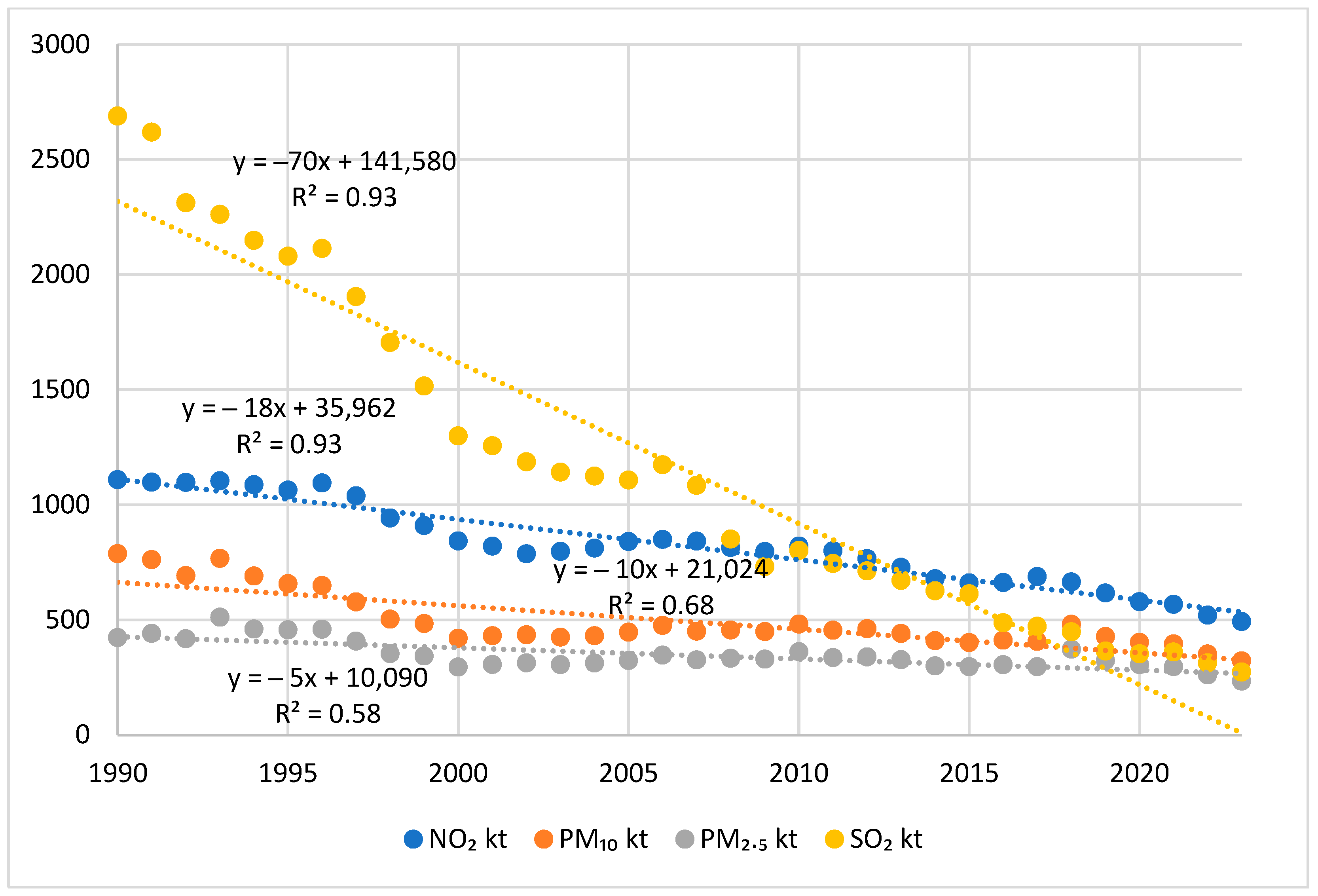
Figure 1. Trends in annual national emissions of SO2, NO2, PM10, and PM2.5 in Poland during the period 1990–2022. Solid lines indicate linear regression fits, along with corresponding regression equations and coefficients of determination (R2) between emissions (kt) and year.
Atmosphere 16 01199 g001
Figure 2. Annual average concentrations (µg·m–3) of four key air pollutants (sulfur dioxide SO2—blue, nitrogen dioxide NO2—orange, particulate matter PM10—grey, particulate matter PM2.5—yellow) measured at ground-level monitoring stations in Poland between 2000 and 2023. The data were retrieved from the national air quality archives maintained by the Chief Inspectorate of Environmental Protection (GIOŚ). Solid lines represent linear regression fits, with corresponding regression equations and coefficients of determination (R2) shown on the graph.
Atmosphere 16 01199 g002
Figure 3. Satellite-derived average concentrations of two air pollutants. NO2 concentrations are displayed as blue bars and SO2 concentrations as an orange line plotted against the secondary (right) y-axis. The x-axis is divided into quarters (e.g., 2020_III marks the third quarter of 2020), covering a full six-year period.
Atmosphere 16 01199 g003
Figure 4. Pearson correlation matrix for SO2, NO2, PM10, and PM2.5 across different data sources. The matrix includes ground-based measurements, national emission inventory data (NIR), and satellite-derived values from Sentinel-5P (Google Earth Engine). Strong positive correlations are marked in red, and negative correlations are marked in blue.
Atmosphere 16 01199 g004
Figure 5. The standardized monthly averages of selected environmental variables (PM2.5, SO2, wind speed, and temperature) from January 2019 to June 2024.
Atmosphere 16 01199 g005
Figure 6. Pearson correlation matrix for SO2, NO2, PM10, and PM2.5, and meteorological variables such as temperature, air humidity, air pressure, and precipitation. The upper triangle shows correlations based on daily data, and the lower triangle shows correlations based on monthly averages. Strong positive correlations are marked in red, and negative correlations are marked in blue.
Atmosphere 16 01199 g006
Figure 7. Scatterplot matrix with LOWESS Smoothing for daily air pollution and meteorological variables (2019–2024), presenting pairwise relationships between pollutants and weather variables with locally weighted trend lines.
Atmosphere 16 01199 g007
Figure 8. Linear regression trend analysis of monthly averaged air pollution and meteorological data (2019–2024), presenting robust linear trends over time for each variable using monthly averages. Red lines indicate trend over time based on linear regression and the numbers in the top right corner of each chart are slopes of regression function which indicate average yearly change of each variable.
Atmosphere 16 01199 g008
Figure 9. Quarterly standardized heatmap (Z-score) of air pollution and meteorological variables (2019–mid-2024), presenting seasonal and long-term patterns across all variables.
Atmosphere 16 01199 g009
Table 1. Summary of key emission sources by pollutant.
PollutantMain SourcesShares in 2023
SO2Power plants, residential heating, heavy industry (especially metallurgy), refineriesAtmosphere 16 01199 i001
NO2Road transport, power generation, industrial combustion, and household heatingAtmosphere 16 01199 i002
PM10Residential heating, industrial processes, road transport (including road dust), constructionAtmosphere 16 01199 i003
PM2.5Residential heating, transport, metallurgy, agriculture (secondary particles), waste burningAtmosphere 16 01199 i004
Table 2. Basic statistics for studied ground-based pollutant data and meteorological variables across all the cities from the beginning of 2019 to the end of June 2024 (Q1—lower quartile, Q3—upper quartile, SD—standard deviation, CV—coefficient of variation).
MeanMedianMin.Max.Q1Q3SDCV
NO2 (μg/m3)19.716.50.191.010.426.112.362.4
PM10 (μg/m3)23.719.81.6207.214.228.714.862.4
PM2.5 (μg/m3)15.112.10.0170.48.218.210.871.7
SO2 (μg/m3)4.53.60.252.22.15.93.477.1
Wind speed (m/s)3.02.80.012.92.03.81.445.5
Temperature (C)9.99.6−19.630.33.816.57.878.7
Air humidity (%)76.077.628.0100.366.986.613.517.8
Air pressure (hPa)997.7997.3954.71045.3988.71006.412.71.3
Precipitation (mm)1.60.00.0130.40.01.34.3266.2
Disclaimer/Publisher’s Note: The statements, opinions and data contained in all publications are solely those of the individual author(s) and contributor(s) and not of MDPI and/or the editor(s). MDPI and/or the editor(s) disclaim responsibility for any injury to people or property resulting from any ideas, methods, instructions or products referred to in the content.