Article

Neural Hierarchical Interpolation for Standardized Precipitation Index Forecasting

by
Rafael Magallanes-Quintanar
1,
Carlos Eric Galván-Tejada
1,
Jorge Isaac Galván-Tejada
1,
Hamurabi Gamboa-Rosales
1,
Santiago de Jesús Méndez-Gallegos
2 and
Antonio García-Domínguez
1,*
1
Unidad Académica de Ingeniería Eléctrica, Universidad Autónoma de Zacatecas, Jardín Juárez 147, Centro, Zacatecas CP 98000, Mexico
2
Campus San Luis Potosí, Colegio de Postgraduados, Salinas de Hidalgo, San Luis Potosí CP 78622, Mexico
*
Author to whom correspondence should be addressed.
Atmosphere 2024, 15(8), 912; https://doi.org/10.3390/atmos15080912
Submission received: 18 June 2024 / Revised: 18 July 2024 / Accepted: 29 July 2024 / Published: 30 July 2024
(This article belongs to the Special Issue Extreme Climate in Arid and Semi-arid Regions)

Abstract

:
In the context of climate change, studying changes in rainfall patterns is a crucial area of research, remarkably so in arid and semi-arid regions due to the susceptibility of human activities to extreme events such as droughts. Employing predictive models to calculate drought indices can be a useful method for the effective characterization of drought conditions. This study applies two type of machine learning methods—long short-term memory (LSTM) and Neural Hierarchical Interpolation for Time Series Forecasting (N-HiTS)—to develop and deploy artificial neural network models with the aim of predicting the regional standardized precipitation index (SPI) in four regions of Zacatecas, Mexico. The predictor variables were a set of climatological time series data spanning from 1964 to 2020. The results suggest that the N-HiTS model outperforms the LSTM model in the prediction and forecasting of SPI time series for all regions in terms of performance metrics: the Mean Squared Error, Mean Absolute Error, Coefficient of Determination and ξ correlation coefficient range from 0.0455 to 0.5472, from 0.1696 to 0.6661, from 0.9162 to 0.9684 and from 0.9222 to 0.9368, respectively, for the regions under study. Consequently, the outcomes revealed the successful performance of the N-HiTS models in accurately predicting the SPI across the four examined regions.

1. Introduction

Time series forecasting is a crucial issue with applications encompassing weather, finance, e-commerce, retailers, and strategic planning among many other fields. Examples of time series forecasting in addressing real-world problems include energy consumption [1], healthcare [2] and traffic prediction [3]. Additionally, early warning systems using time series are noteworthy examples aiding in addressing vulnerabilities associated with weather events such as extreme rainfalls and droughts [4,5]. Drought is a prolonged period of abnormally low rainfall, leading to a shortage of water. This natural phenomenon plays a critical role in shaping ecosystems, affecting water availability, agricultural productivity, and socio-economic stability. The scientific study of drought encompasses its physical, social, and biological dimensions, each contributing to a comprehensive understanding of its impacts and management strategies [6]. Moreover, there is moderate confidence that droughts will become more severe in the 21st century during certain seasons and in specific regions, due to decreased precipitation and/or increased evapotranspiration [5,6].
In the context of arid and semi-arid regions, various methods have been devised to evaluate droughts, with drought indices standing out as widely utilized. The standardized precipitation index (SPI) allows us to classify the observed time series rainfall based on its standardized deviation from a rainfall probability distribution function [7]. Since persistent drought is a severe problem in north-central Mexico, by examining SPI data as a time series signal, utilizing time series forecasting methods to anticipate forthcoming drought levels is viable.
There are generally two primary classifications for time series forecasting (TSF) approaches: conventional statistics/econometrics methods and machine learning methods. Recently, machine learning methods (which are a type of AI) have become more proficient, precise, and user-friendly, making them particularly useful for analyzing hydrological data [8,9]. Neural networks, which are an information processing technique that learns from data, have been successfully used to model and predict nonlinear time series in various fields, including water resources and hydrology [4]. Consequently, artificial neural network (ANN) models have been employed as a valuable data-driven tool for forecasting monthly SPI time series [10,11,12,13,14,15,16,17].
Among machine learning methods, long short-term memory (LSTM) [18], stands as a prominent form of recurrent neural network (RNN) architecture, specifically designed to address the challenges associated with long-term dependencies, such as those found in climatological time series data. The LSTM approach is very effective in the task of modeling and predicting time series due to their ability to remember relevant information over extended periods of time. On the other hand, certain constraints and disadvantages of forecasting methodologies rooted in machine learning, such as the LSTM approach, could encompass computationally intensive and unstable training stages, managing a considerable set of hyperparameters, and susceptibility to the initialization of random weights. Furthermore, long-horizon forecasting is an additional challenge when dealing with TSF when using neural networks.
To deal with the aforementioned problems, Neural Hierarchical Interpolation for Time Series Forecasting (N-HiTS) was proposed [19]. Essentially, the N-HiTS approach involves employing multi-rate sampling for the input signal and conducting a multi-scale synthesis of the forecast. This leads to a hierarchical construction of predictions, significantly lowering computational workload and enhancing the final forecasting accuracy.
In this paper, to realize neural networks’ potential, we used long-time series of precipitation (1964–2020) recorded in north-central Mexico. Our main objectives were (a) to compute SPI and use it as a time series signal to test the prediction of SPI by means of LSTM and NHiTS approaches, (b) to compare LSTM results against NHiTS results using well-known metrics, and (c) to forecast the regional standardized precipitation index for 24 months (near future) using the best neural forecasting method.

2. Materials and Methods

2.1. Study Region and Datasets

Zacatecas state is situated in north-central Mexico between coordinates 21.016 and 25.116 N and 100.716 and 104.366 W; it has a surface area of 75,284 km2, which represents 3.8% of the national territory, and has a population of 1,579,209 people, with 59% living in urban areas and 41% in rural areas. The state features a cold, dry climate, with 75% of its territory being arid or semi-arid and an average annual rainfall of 420 mm. The local vegetation includes shrubs, grasses, mesquite and huizache trees, and various species of cacti. The primary economic activities are silver mining, trade, agriculture (notably beans and fodder), and livestock farming (particularly cattle). Zacatecas also experiences high rates of international migration, with 4.8% of its population living abroad. In this study, we analyzed 31 sets of monthly rainfall data utilizing a long-term dataset (1964–2020) from weather stations located within the territory of Mexico’s state of Zacatecas (Figure 1). The precipitation data were provided by the ‘Comisión Nacional del Agua,’ which serves as Mexico’s official national authority responsible for preserving weather and climate data records. Before any processing, we scrutinized the rainfall datasets to ensure that outliers, missing values, or record error values were not included in the analysis.
After scrutinizing the rainfall time series, the resulting dataset was used to compute time series of the standardized precipitation index.

2.2. Standardized Precipitation Index

The standardized precipitation index (SPI) [7] is a well-established tool used to measure the severity of precipitation anomalies over different timescales. To monitor and evaluate the prevailing drought conditions, the SPI is extensively employed. The SPI uses only precipitation data to calculate a standardized value that represents the deviation of the current precipitation from the long-term average for a given location and time period. The computation of the standardized value involves dividing the deviation between the current precipitation and the long-term average by the standard deviation of the long-term precipitation. The final SPI result is a value that is expressed in units of standard deviations from the long-term mean.
The computed SPI values could be classified into categories based on their magnitude, with negative values indicating drier-than-average conditions and positive values indicating wetter-than-average conditions [7]. Table 1 displays the categorization of SPI values, ranging from “extremely dry” to “extremely wet,” as well as intermediate classes indicating moderate to severe drought or wet conditions [7].
Since changes in precipitation quantity affect different facets of the hydrological cycle, SPI computation employs multiple timescales [20]. The SPI values over a 3-month period characterize moisture conditions in the short and medium term, while the 6-month-scale SPI values indicate droughts that impact agriculture. Moreover, SPI values over a 12-month period indicate droughts that affect aquifers or groundwater levels. In this study, we calculated SPI values over a 12-month timescale [21].
In this work, SPI computation was conducted using R system version 4.3.2 [22] and the ‘SPEI’ package version 1.8.1 [23]. Both the system and package can be downloaded through the Comprehensive R Archive Network [24].

Cluster Analysis

Cluster analysis serves as a powerful statistical method for identifying coherent climate zones using observed meteorological data [25,26]. This technique organizes data points based on the inherent characteristics of the data and their interconnections. The objective is to ensure that objects within a cluster exhibit likeness while being distinct from those in other clusters [27]. The stronger the coherence within clusters and the disparity between them, the more refined or differentiated the clustering outcome [27].
In this research, a tree clustering algorithm was employed to group items (specifically, monthly SPI time series) into larger clusters (representing regions with similar SPI values, i.e., precipitation patterns). The Canberra distance served as the criterion for linkage, while Ward’s method was applied as the rule for linking clusters.
The cluster analysis was conducted using the R system version 4.3.2 [22], along with the ‘hclust’ package [22] and the ‘ape’ package [28]. Both the system and packages can be downloaded through the Comprehensive R Archive Network [24].

2.3. Neural Time Series Forecasting

Besides the classical statistics/econometrics methods for climatological TSF, machine learning methods are a feasible option. Studies indicate that artificial neural networks (ANNs) might offer a more effective alternative to conventional methods for modeling nonlinear time series data [29]. Moreover, some findings indicate that among available TSF options, long short-term memory (LSTM) and convolutional networks (CNNs) stand out as the top choices, with LSTMs emerging as the most effective in generating accurate TSF [30].

2.3.1. Long Short-Term Memory Networks

LSTMs were introduced as a solution for the challenges faced by the Elman Recurrent Neural Networks (ERNNs) used to address the task of handling temporal patterns within datasets [18]. One advantage of LSTMs is the fact that they possess the ability to capture temporal relationships over extended time frames without disregarding short-term patterns.
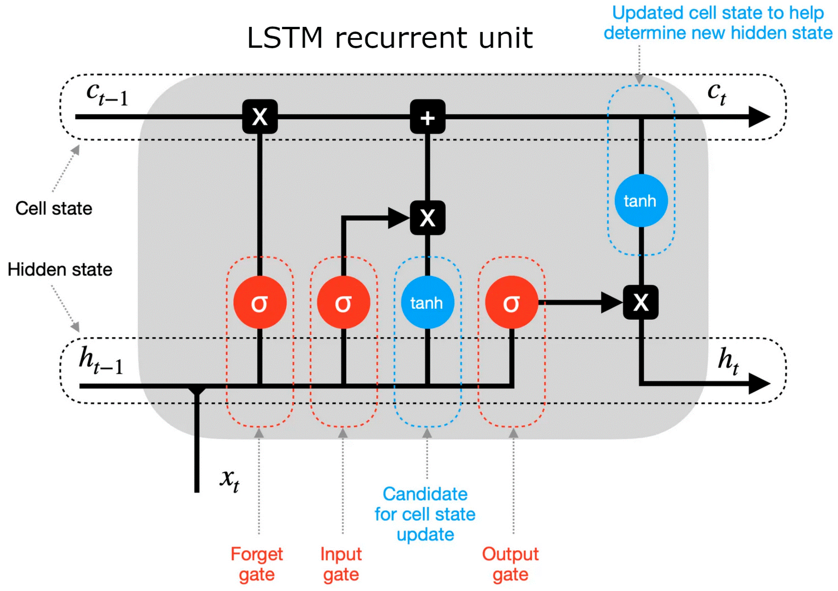
By definition, the LSTM model comprises three key components: an input gate, a forget gate, and an output gate. These gates are pivotal in controlling the information flow into, out of, and within the memory cell. As a result, LSTM has the capability to preserve temporal information within the state over an extended number of time steps, making it a popular choice for analyzing, predicting, and classifying sequential data (i.e., time series) across both univariate and multivariate domains.
As depicted in Figure 2, the architecture of an LSTM model employs a series of equations including the forget gate, input gate, candidate activation, cell state update, and output gate, respectively [31]:
f t = σ W f h t 1 , x t + b f ,
i t = σ W i h t 1 , x t + b i ,
C t ~ = t a n h W c h t 1 , x t + b c ,
C t = σ f t C t 1 + i t C t ~ ,
o t = σ W o h t 1 , x t + b o .
where xt is the input at time step t, ht−1 is the hidden state from the preceding time step, σ represents a logistic sigmoid function, and ∗ symbolizes element-wise multiplication. Weight (Wf, Wi, WC, Wo) and bias (bf, bi, bC, bo) are model parameters to be learned during the training phase [31].
In this work, the LSTM approach was applied with the aim of forecasting SPI regional time series by means of the Neuralforecast library implemented in Python [32].

2.3.2. Neural Hierarchical Interpolation for Time Series Forecasting

The Neural Hierarchical Interpolation for Time Series Forecasting (N-HiTS) model was proposed with the aim of improving the performance of large-scale forecasting systems and dealing with long-horizon time series predictions [19]. The N-HiTS approach tackles both obstacles using hierarchical interpolation methods and multi-rate data sampling techniques. As a summary, multi-rate data sampling can learn short-term and long-term effects in the series by adaptively adjusting the sampling rates. The hierarchical interpolation allows the model to effectively capture the hierarchical relationships present in the time series data. As a result, the model integrates forecasts generated across various time frames, combining both long-term and short-term effects. The architecture of the N-HiTS model is shown in Figure 3.
Following [19] and the N-HiTS model architecture (Figure 3) as a reference, let yt be the SPI value at time t. Then, y t L : t is a vector of the SPI with L lags. Let y ~ t L : t , b be the backcast and let y ~ t L : t + H , b   be the forecast of the b-th block. Considering the s-th stack, let y t L : t , s be the stack residual and let y ~ t L : t , l be the forecast. Finally, the global forecast of the SPI using the N-HiTS model is y ^ t + 1 : t + H .

Multi-Rate Signal Sampling

As depicted in Figure 3, the N-HiTS model takes in the input y t L : t , which initially proceeds to the initial block of the first stack. Within each block, including the first one, a MaxPool layer with a kernel size of kb is employed to identify the significant elements of the input. While a smaller kernel size permits the utilization of a greater number of high-frequency components from the data, a larger kernel size filters out more high-frequency elements from the time series data. Consequently, the Multilayer Perceptron (MLP) in block b will be compelled to concentrate on acquiring either low- or high-frequency patterns, in agreement with the selected kernel size. This process is called Multi-Rate Signal Sampling (MRSS) and additionally enables the N-HiTS model to accelerate the training phase by reducing the input size of the MLP in block b, thereby diminishing the number of parameters for the MLP and mitigating the risks of overfitting. According to the above process, MRSS is defined as
y ( p ) t L : t , b = M a x P o o l y t L : t , b , k b .

Nonlinear Regression

After subsampling, block b examines its input and nonlinearly computes forward θ l f and backward θ f b   interpolation MLP coefficients by regression, which learn a hidden vector hl that is subsequently linearly projected:
h l = M L P l y t L : t , l ( p ) ,
θ l f = L I N E A R f ( h l ) ,
θ l b = L I N E A R b h l .
The coefficients are subsequently employed to generate the backcast y ~ t L : t , l   and forecast y ^ t L : t , l   outputs of the block, following the described procedure. After this, the forecasts will be aggregated to generate the forecast for the s-th stack. Following this, by deducting the most recent backcast residual from the input signal, the input for the next stack (s + 1-th stack) is computed as follows:
y t + 1 : t + H , s = b = 1 B y ^ t + 1 : t + H , b ,
y t L : t , s = y t L : t , B y ^ t L : t , B .

Hierarchical Interpolation

N-HiTS applies a method named Temporal Interpolation (TI) as introduced in [19] to mitigate the escalating computational demands associated with other neural network multi-horizon forecasting models, particularly when the forecast horizon H increases. Consider rl as the dimensionality or expressiveness ratio of the interpolation parameters, determining the parameter count for each unit of output time, | θ f b | = r l H . To restore the initial sampling rate and forecast all H points within the horizon, the TI is executed through the interpolation function denoted as g:
y ^ τ , b = g τ , θ f b , τ t + 1 , , t + H ,
y ~ τ , b = g τ , θ b b , τ t L , , t .
Note that g represents an interpolation function, which may take the form of nearest neighbor, piecewise linear, or cubic interpolation. For the sake of simplicity, g represents the linear interpolator (g   C 1 ) as interpolation can vary in smoothness. Along with the time partition T = t + 1 ,   t + 1 + 1 r l , , t + H 1 r l , t + H , g is expressed as
g τ , θ = θ t 1 + θ t 2 θ t 1 t 2 t 1 τ t 1 .
where
t 1 = a r g m i n t T : t τ τ t ,
t 2 = t 1 + 1 r l .
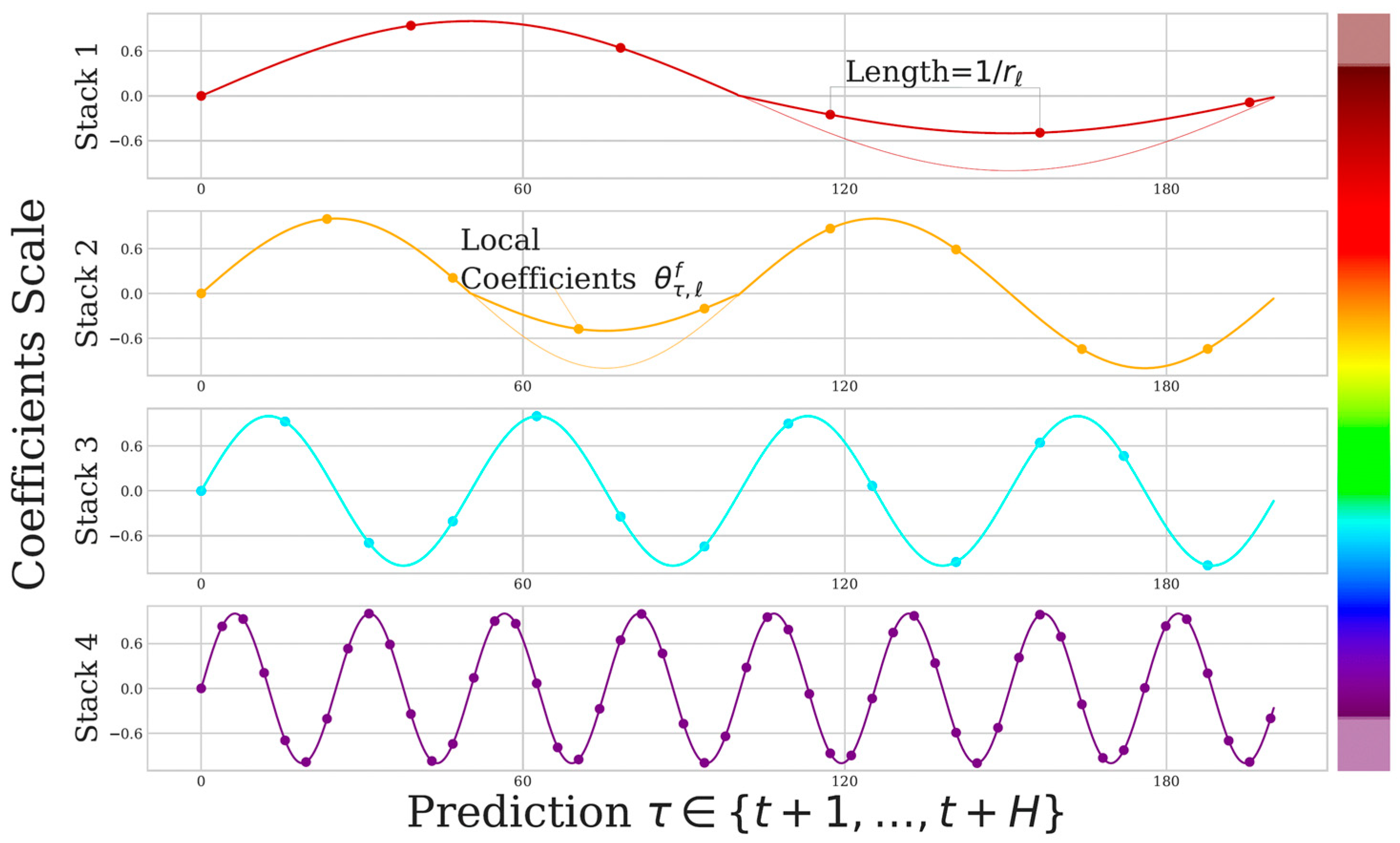
The hierarchical interpolation method enhances MRSS by strategically distributing expressiveness ratios among different blocks. Blocks in proximity to the input have smaller rl and larger kl, indicating that input blocks produce signals of lower granularity through more enhanced interpolation, as they are compelled to examine signals that are more enhanced, sub-sampled, and smoothed. The resultant hierarchical forecast y ^ t + 1 : t + H is constructed by aggregating the outputs of all blocks, essentially forming it through interpolations across various levels of the time-scale hierarchy. As each block specializes in its unique scale of input and output signals, this creates a well-defined hierarchical structure of interpolation granularity, as illustrated in Figure 4. Alternatively, each stack can focus on modeling a distinct recognized cycle within the time series such as monthly, weekly, etc., using a corresponding rl. Finally, [19] established the theoretical guarantees of the hierarchical interpolation technique, demonstrating that this approach is not just empirically potent and resilient.
In this work, the N-HiTS approach was applied with the aim of forecasting SPI regional time series by means of the Neuralforecast library implemented in Python [32]. The Neuralforecast library is part of Nixtlaverse [33], which is a collection of open-source libraries designed to develop accurate and effective models, with a strong focus on usability and specializing in several characteristics of TSF.

2.3.3. Forecasting Performance

To effectively assess the forecasting performance of the models, this study used the following well-known error metrics: Mean Absolute Error (MAE), Mean Square Error (MSE), determination coefficient (R2) and ξ correlation coefficient.
M A E = 1 n i = 1 n S P I p i S P I o i ,
M S E = 1 n i = 1 n S P I p i S P I o i 2 .
MAE quantifies the average deviation between predicted and observed values, offering insights into the models’ long-term performance. Lower MAE values indicate superior long-term predictive capability. MSE gauges the disparity between observed and calculated values, with lower MSE values signifying greater prediction accuracy. The determination coefficient, R2, serves as an efficiency criterion, illustrating the proportion of initial uncertainty elucidated by the model. The final assessment metric, ξ, is a new correlation coefficient that is a consistent estimator of a certain measure of dependence between the random variables X and Y [34].
An ideal model would exhibit minimal MSE and MAE, indicative of minimal accumulated errors. Achieving MSE = 0, R2 = 1, and ξ = 1, reflecting a perfect fit between observed and calculated values, is improbable but represents the optimal scenario.
In this research, the ξ correlation coefficient was computed using the R system version 4.3.2 [22] along with the ‘XICOR’ package [35]. Both the system and package can be downloaded through the Comprehensive R Archive Network [24].
Finally, we employed the difference between observed and predicted SPI values to gauge the model’s prediction error (PE).
P E = S P I o i S P I p i .
It is important to note that in the training of multilayer networks, a common approach involves dividing the data into three distinct subsets. The initial subset, known as the training set, is utilized for gradient computation and updating the network’s weights and biases. Following this, the second subset, referred to as the validation set, is employed to monitor the error throughout the training procedure. In the early stages of training, the validation error generally decreases, mirroring the trend seen in the training set error. Finally, the test set is used to evaluate the trained model’s final performance, providing an unbiased assessment of its capabilities on independent or unseen datasets.
In this study, both the LSTM and N-HiTS models used 520 months (80% of sample length) for training and 129 months (20% of sample length) for validation. Furthermore, the final 24 observed true SPI values were used as a testing sample against the forecasted values. The previous procedure was applied in the SPI time series for each one of the regions detected using the clustering technique.

3. Results and Discussion

The original 31 time series of rainfall were used to compute their corresponding SPI time series. The result of using the clustering technique on the whole SPI time series database was a set of four regions (Semi-arid, High plain, Mountains and Canyons) based on the similarity of their SPI values.
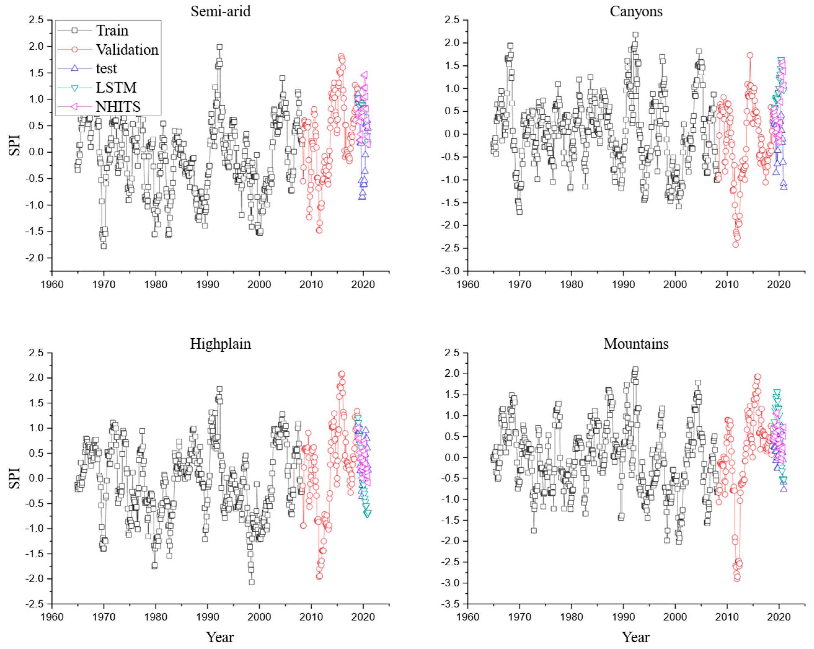
The set of four regional SPI time series were used as model input using the LSTM and N-HiTS approaches for SPI time series prediction. Figure 5 displays the plot of observed (train, validation, and test) values of SPI as well as the SPI forecasting results of the LSTM and N-HiTS models for semi-arid, High plain, Mountain and Canyon regions.
The results of training and validating the ANNs when considering the metrics MSE and MAE revealed lower values for the N-HiTS model than the LSTM model in all the regions under study, as shown in Table 2. It is evident from the results that the N-HiTS model’s MSE performance (0.3406) was better than the LSTM model’s MSE performance (0.7452) for all regional SPI time series. The same occurs when considering the MAE metric: the N-HiTS model’s performance was 0.4744 against the LSTM model’s MSE performance of 0.7158. In particular, the better performance of the N-HiTS model occurred in the Highland region, which showed the lowest values for both the MSE and MAE metrics. Conversely, considering only the results of the N-HiTS model for all the analyzed regions, the lowest performance was that of the Mountain region, with higher MSE and MAE values.
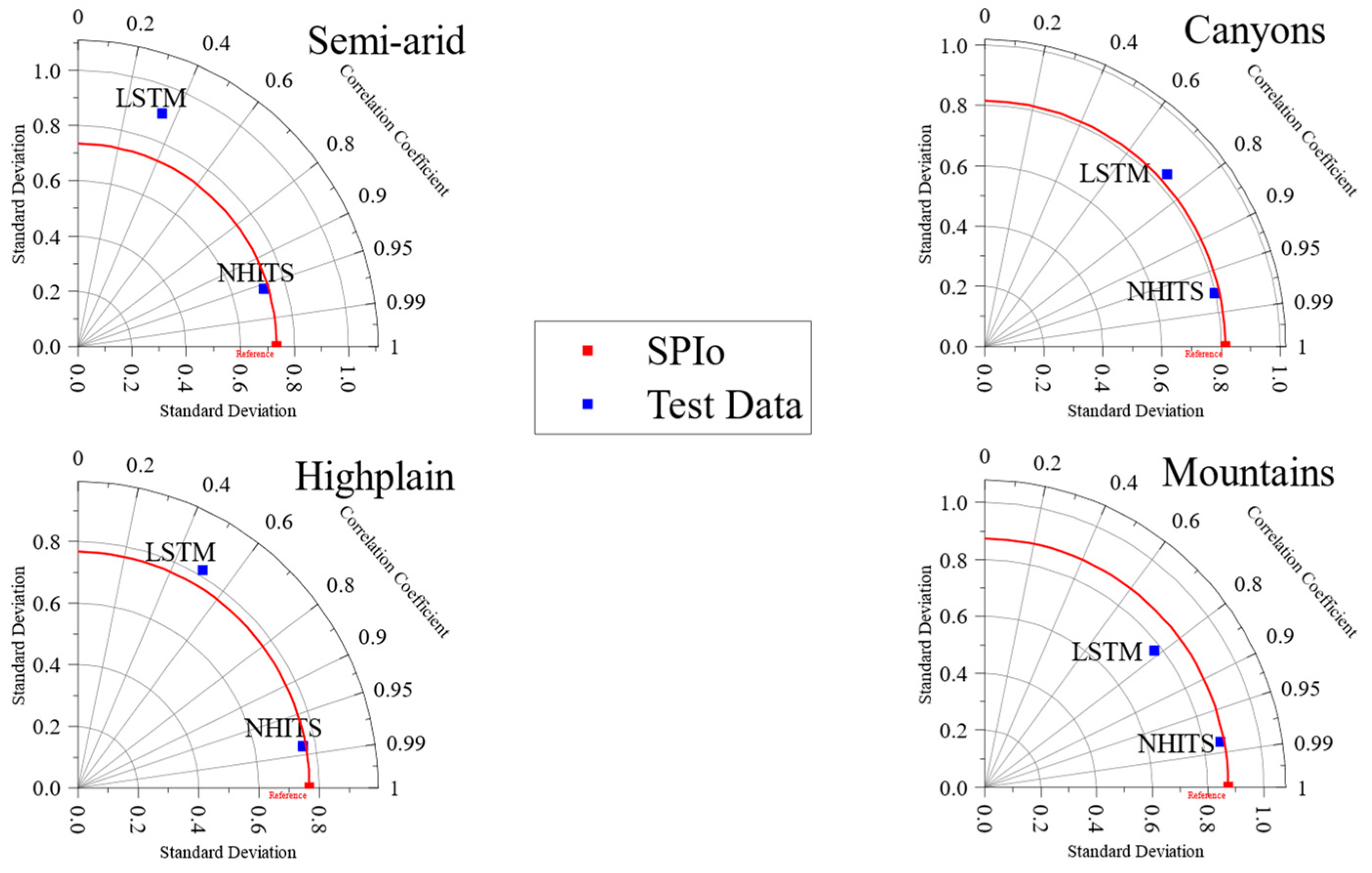
The Taylor diagram (Figure 6) illustrates that the N-HiTS model outperforms the LSTM model in predicting the standardized precipitation index (SPI) across all analyzed regions. N-HiTS consistently achieves higher correlation coefficients (above 0.95) and low standard deviation values near to the observed SPI or reference values, indicating strong agreement with observed data and reliable predictions. In contrast, the LSTM model shows lower correlation coefficients, particularly in the semi-arid and High plain regions, and higher standard deviations, reflecting greater variability and less accurate predictions. Overall, the N-HiTS model demonstrates superior predictive capability and reliability in diverse climatic conditions.
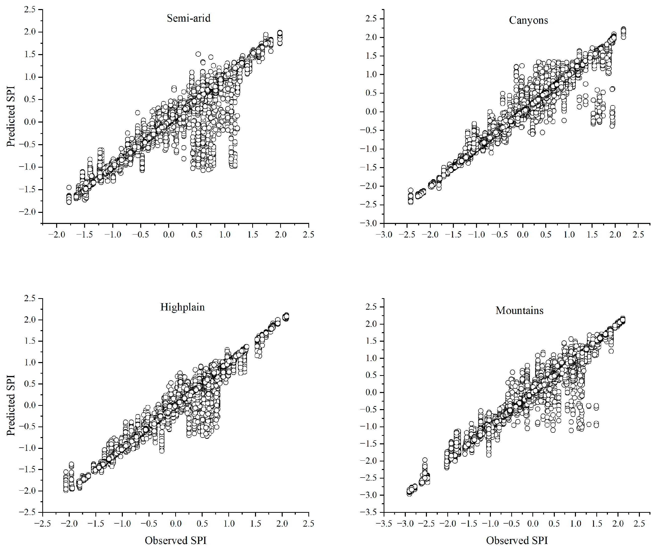
Additionally, the performance of the LSTM and N-HiTS in the four regions was analyzed through a linear correlation analysis considering the scatter plot between the observed SPI and the predicted SPI values during the analyzed period. The results of the determination coefficient (R2) and correlation coefficient (ξ) are shown in Table 3.
As the N-HiTS determination coefficient (R2) and correlation coefficient (ξ) values were better than their corresponding LSTM values in all analyzed regional SPI time series, only the scatter plots of N-HiTS-observed SPI versus predicted SPI values are displayed in Figure 7.
The probability under normal distribution of the prediction error of the N-HiTS models is summarized in Table 4 and shows the under-prediction (PE < 0) and over-prediction (PE > 0) skills. The error will be zero when the predicted SPI value exactly matches the SPI observed value [36]. The results show that instances where PE < 0 are more frequent than instances where PE > 0 in every region except for semi-arid regions. These results indicate that N-HiTS models under-predicted the SPI for all regions except for semi-arid regions. The greatest discrepancy was observed in the Mountain region, with a probability of 56.36%, while the smallest discrepancy, 42.41%, occurred in the semi-arid region. Additionally, the minimum probability of over-prediction, 43.64%, was observed in the Mountain region, while the maximum probability of over-prediction error, 57.59%, was found in the semi-arid region. These results are consistent with the determination coefficients of the linear models comparing predicted and observed SPI values (Table 3).
LSTMs are often used in time series forecasting [37,38] because they excel in capturing long-term temporal dependencies and retain short-term patterns effectively. However, the LSTM approach has some disadvantages; for example, MLP networks fail to effectively capture the temporal sequencing within time series data, resulting in poor predictive performance [29].
Otherwise, N-HiTS enables the sequential assembly of predictions, highlighting components with varying frequencies and scales. It achieves this by decomposing the input signal and synthesizing the forecast. N-HiTS has been tested using publicly available datasets against several models successfully [19], resulting in an average accuracy improvement over the latest Transformer architectures.
Our results imply that the N-HiTS model outperforms the LSTM model in the prediction and forecasting of SPI time series for all regions in the analyzed time period considering the metrics MSE, MAE, R2, and ξ.
Overall, the N-HiTS models exhibited a satisfactory degree of predictive accuracy for SPI. Our findings align favorably with the outcomes reported by [8,11,15,16,39], who effectively utilized artificial neural network approaches to forecast the monthly standardized precipitation index.
Furthermore, our results build upon those of [40] by introducing an approach that not only enables the delineation of smaller and more detailed regional climatic zones in Mexico using the SPI but also establishes a framework for forecasting SPI values by means of the N-HiTS approach.
Notably, this is the first study, to our knowledge, that applies the N-HiTS model for monthly standardized precipitation index prediction as well as the new correlation coefficient ξ. Moreover, the N-HiTS model, characterized by low computing costs and satisfactory performance, has the potential to be suitable as an important state-of-the-art tool for drought prediction, that is, the detection of climatic and agricultural risks caused by drought in the context of extreme climate in arid and semi-arid regions.

4. Conclusions

Recently, forecasting drought has emerged as a significant concern across meteorology, hydrology, water resource management, and sustainable agriculture due to the connection between human activities and water utilization. We developed AI models using LSTM and N-HiTS approaches with the aim to predict the values of four monthly standardized precipitation index time series belonging to the territory of Zacatecas state in north-central Mexico.
According to the evaluation metrics, our analysis suggests that the N-HiTS model’s approach notably outperforms that of the LSTM model, providing evidence that the N-HiTS model serves as a valuable AI tool for predicting monthly SPI values.
Regarding the matter of climate change, the use of the N-HiTS model for drought prediction in future research could provide valuable information for decision making. Considering that this research deals with univariate time series, upcoming studies should compare the N-HiTS model approach against various ANN models, training algorithms, and framework methodologies to measure its effectiveness in different scenarios using other climatological variables by means of multivariate time series.

Author Contributions

Conceptualization, R.M.-Q.; data curation, R.M.-Q.; formal analysis, R.M.-Q. and C.E.G.-T.; funding acquisition, H.G.-R.; investigation, R.M.-Q., J.I.G.-T. and S.d.J.M.-G.; methodology, R.M.-Q.; project administration, R.M.-Q. and A.G.-D.; resources, R.M.-Q.; software, R.M.-Q. and J.I.G.-T.; supervision, R.M.-Q.; validation, R.M.-Q. and C.E.G.-T.; visualization, R.M.-Q.; writing—original draft, R.M.-Q.; writing—review and editing, R.M.-Q. and A.G.-D. All authors have read and agreed to the published version of the manuscript.

Funding

This research received no external funding.

Institutional Review Board Statement

Not applicable.

Informed Consent Statement

Not applicable.

Data Availability Statement

The database used to support the findings of this study is called “Proyecto de bases de datos climatológicos”, and was supplied by the “Comisión Nacional del Agua”, the national official institution in charge of climatic and meteorological data record-keeping in Mexico. Data are available at https://drive.google.com/drive/folders/10HCD7X_-sgTIJSQnJE9SkFL92ca3ERDC accessed on 15 May 2024.

Conflicts of Interest

The authors declare no conflicts of interest.

References

  1. Liu, H.; Liu, Y.; Guo, X.; Wu, H.; Wang, H.; Liu, Y. An Energy Consumption Prediction Method for HVAC Systems Using Energy Storage Based on Time Series Shifting and Deep Learning. Energy Build. 2023, 298, 113508. [Google Scholar] [CrossRef]
  2. Kaushik, S.; Choudhury, A.; Sheron, P.K.; Dasgupta, N.; Natarajan, S.; Pickett, L.A.; Dutt, V. AI in Healthcare: Time-Series Forecasting Using Statistical, Neural, and Ensemble Architectures. Front. Big Data 2020, 3, 4. [Google Scholar] [CrossRef] [PubMed]
  3. Shuvo, M.A.R.; Zubair, M.; Purnota, A.T.; Hossain, S.; Hossain, M.I. Traffic Forecasting Using Time-Series Analysis. In Proceedings of the 2021 6th International Conference on Inventive Computation Technologies (ICICT), Coimbatore, India, 20 January 2021; pp. 269–274. [Google Scholar]
  4. Basher, R. Global Early Warning Systems for Natural Hazards: Systematic and People-Centred. Phil. Trans. R. Soc. A 2006, 364, 2167–2182. [Google Scholar] [CrossRef] [PubMed]
  5. Field, C.B. Managing the Risks of Extreme Events and Disasters to Advance Climate Change Adaptation: Special Report of the Intergovernmental Panel on Climate Change; Cambridge University Press: Cambridge, UK, 2012; ISBN 1-107-02506-0. [Google Scholar]
  6. Bonaldo, D.; Bellafiore, D.; Ferrarin, C.; Ferretti, R.; Ricchi, A.; Sangelantoni, L.; Vitelletti, M.L. The Summer 2022 Drought: A Taste of Future Climate for the Po Valley (Italy)? Reg. Env. Change 2023, 23, 1. [Google Scholar] [CrossRef]
  7. McKee, T.B.; Doesken, N.J.; Kleist, J. The Relationship of Drought Frequency and Duration to Time Scales. In Proceedings of the 8th Conference on Applied Climatology, Anaheim, CA, USA, 17–22 January 1993; Volume 17, pp. 179–183. [Google Scholar]
  8. Poornima, S.; Pushpalatha, M. Drought Prediction Based on SPI and SPEI with Varying Timescales Using LSTM Recurrent Neural Network. Soft Comput. 2019, 23, 8399–8412. [Google Scholar] [CrossRef]
  9. Chen, L.; Han, B.; Wang, X.; Zhao, J.; Yang, W.; Yang, Z. Machine Learning Methods in Weather and Climate Applications: A Survey. Appl. Sci. 2023, 13, 12019. [Google Scholar] [CrossRef]
  10. Choubin, B.; Malekian, A.; Golshan, M. Application of Several Data-Driven Techniques to Predict a Standardized Precipitation Index. Atmosfera 2016, 29, 121–128. [Google Scholar] [CrossRef]
  11. Ali, Z.; Hussain, I.; Faisal, M.; Nazir, H.M.; Hussain, T.; Shad, M.Y.; Mohamd Shoukry, A.; Hussain Gani, S. Forecasting Drought Using Multilayer Perceptron Artificial Neural Network Model. Adv. Meteorol. 2017, 2017, 5681308. [Google Scholar] [CrossRef]
  12. Ozger, M.; Mishra, A.K.; Singh, V.P. Estimating Palmer Drought Severity Index Using a Wavelet Fuzzy Logic Model Based on Meteorological Variables. Int. J. Climatol. 2011, 31, 2021–2032. [Google Scholar] [CrossRef]
  13. Masinde, M. Artificial Neural Networks Models for Predicting Effective Drought Index: Factoring Effects of Rainfall Variability. Mitig. Adapt. Strateg. Glob. Change 2014, 19, 1139–1162. [Google Scholar] [CrossRef]
  14. Belayneh, A.; Adamowski, J.; Khalil, B.; Ozga-Zielinski, B. Long-Term SPI Drought Forecasting in the Awash River Basin in Ethiopia UsingWavelet Neural Network andWavelet Support Vector Regression Models. J. Hydrol. 2014, 508, 418–429. [Google Scholar] [CrossRef]
  15. Deo, R.C.; Sahin, M. Application of the Artificial Neural Network Model for Prediction of Monthly Standardized Precipitationband Evapotranspiration Index Using Hydrometeorological Parameters and Climate Indices in Eastern Australia. Atmos. Res. 2015, 161–162, 65–81. [Google Scholar] [CrossRef]
  16. Soh, Y.W.; Koo, C.H.; Huang, Y.F.; Fung, K.F. Application of Artificial Intelligence Models for the Prediction of Standardized Precipitation Evapotranspiration Index (SPEI) at Langat River Basin, Malaysia. Comput. Electron. Agric. 2018, 144, 164–173. [Google Scholar] [CrossRef]
  17. Magallanes-Quintanar, R.; Galván-Tejada, C.E.; Galvan-Tejada, J.I.; Méndez-Gallegos, S.d.J.; Blanco-Macías, F.; Valdez-Cepeda, R.D. Artificial Neural Network Models for Prediction of Standardized Precipitation Index in Central Mexico. Agrociencia 2023, 57, 11–20. [Google Scholar] [CrossRef]
  18. Hochreiter, S.; Schmidhuber, J. Long Short-Term Memory. Neural Comput. 1997, 9, 1735–1780. [Google Scholar] [CrossRef]
  19. Challu, C.; Olivares, K.G.; Oreshkin, B.N.; Ramirez, F.G.; Canseco, M.M.; Dubrawski, A. Nhits: Neural Hierarchical Interpolation for Time Series Forecasting. Proc. AAAI Conf. Artif. Intell. 2023, 37, 6989–6997. [Google Scholar] [CrossRef]
  20. Koudahe, K.; Kayode, A.J.; Samson, A.O.; Adebola, A.A.; Djaman, K. Trend Analysis in Standardized Precipitation Index and Standardized Anomaly Index in the Context of Climate Change in Southern Togo. Atmos. Clim. Sci. 2017, 7, 401–423. [Google Scholar] [CrossRef]
  21. Caloiero, T. Drought Analysis in New Zealand Using the Standardized Precipitation Index. Environ. Earth Sci. 2017, 76, 569. [Google Scholar] [CrossRef]
  22. R CoreTeam. R: A Language and Environment for Statistical Computing; R Foundation for Statistical Computing: Vienna, Austria, 2013. [Google Scholar]
  23. Beguería, S.; Vicente-Serrano, S.M. SPEI: Calculation of the Standardized Precipitation-Evapotranspiration Index. In R Package Version 1.8.1 2017; R Foundation for Statistical Computing: Vienna, Austria, 2017; Volume 1. [Google Scholar]
  24. The Comprehensive R Archive Network. Available online: https://cran.r-project.org/ (accessed on 1 June 2024).
  25. Unal, Y.; Kindap, T.; Karaca, M. Redefining the Climate Zones of Turkey Using Cluster Analysis. Intl. J. Climatol. 2003, 23, 1045–1055. [Google Scholar] [CrossRef]
  26. Karmalkar, A.V.; Bradley, R.S.; Diaz, H.F. Climate Change in Central America and Mexico: Regional Climate Model Validation and Climate Change Projections. Clim. Dyn. 2011, 37, 605–629. [Google Scholar] [CrossRef]
  27. Tan, P.-N.; Kumar, V. Introduction to Data Mining; Pearson: London, UK, 2018; ISBN 978-0133128901. [Google Scholar]
  28. Paradis, E.; Schliep, K. Ape 5.0: An Environment for Modern Phylogenetics and Evolutionary Analyses in R. Bioinformatics 2019, 35, 526–528. [Google Scholar] [CrossRef] [PubMed]
  29. Farajzadeh, J.; Fakheri Fard, A.; Lotfi, S. Modeling of Monthly Rainfall and Runoff of Urmia Lake Basin Using “Feed-Forward Neural Network” and “Time Series Analysis” Model. Water Resour. Ind. 2014, 7–8, 38–48. [Google Scholar] [CrossRef]
  30. Lara-Benítez, P.; Carranza-García, M.; Riquelme, J.C. An Experimental Review on Deep Learning Architectures for Time Series Forecasting. Int. J. Neural Syst. 2021, 31, 2130001. [Google Scholar] [CrossRef] [PubMed]
  31. Shenfield, A.; Howarth, M. A Novel Deep Learning Model for the Detection and Identification of Rolling Element-Bearing Faults. Sensors 2020, 20, 5112. [Google Scholar] [CrossRef] [PubMed]
  32. Olivares, K.G.; Challú, C.; Garza, F.; Canseco, M.M.; Dubrawski, A. NeuralForecast: User Friendly State-of-the-Art Neural Forecasting Models. PyCon Salt Lake City Utah US 2022, 2022, 6. [Google Scholar]
  33. Nixtla. Available online: https://nixtlaverse.nixtla.io/ (accessed on 1 June 2024).
  34. Chatterjee, S. A New Coefficient of Correlation. J. Am. Stat. Assoc. 2021, 116, 2009–2022. [Google Scholar] [CrossRef]
  35. Chatterjee, S.; Holmes, S. XICOR. In R Package Version 0.4.1 2023; R Foundation for Statistical Computing: Vienna, Austria, 2023; Volume 1. [Google Scholar]
  36. Moustris, K.P.; Larissi, I.K.; Nastos, P.T.; Paliatsos, A.G. Precipitation Forecast Using Artificial Neural Networks in Specific Regions of Greece. Water Resour. Manag. 2011, 25, 1979–1993. [Google Scholar] [CrossRef]
  37. Smyl, S. A Hybrid Method of Exponential Smoothing and Recurrent Neural Networks for Time Series Forecasting. Int. J. Forecast. 2020, 36, 75–85. [Google Scholar] [CrossRef]
  38. Bandara, K.; Bergmeir, C.; Smyl, S. Forecasting across Time Series Databases Using Recurrent Neural Networks on Groups of Similar Series: A Clustering Approach. Expert Syst. Appl. 2020, 140, 112896. [Google Scholar] [CrossRef]
  39. Magallanes-Quintanar, R.; Galván-Tejada, C.E.; Galván-Tejada, J.I.; Méndez-Gallegos, S.d.J.; García-Domínguez, A.; Gamboa-Rosales, H. Narx Neural Networks Models for Prediction of Standardized Precipitation Index in Central Mexico. Atmosphere 2022, 13, 1254. [Google Scholar] [CrossRef]
  40. Giddings, L.; Soto, M.; Rutherford, B.M.; Maarouf, A. Standardized Precipitation Index Zones for México. Atmosfera 2005, 18, 33–56. [Google Scholar]
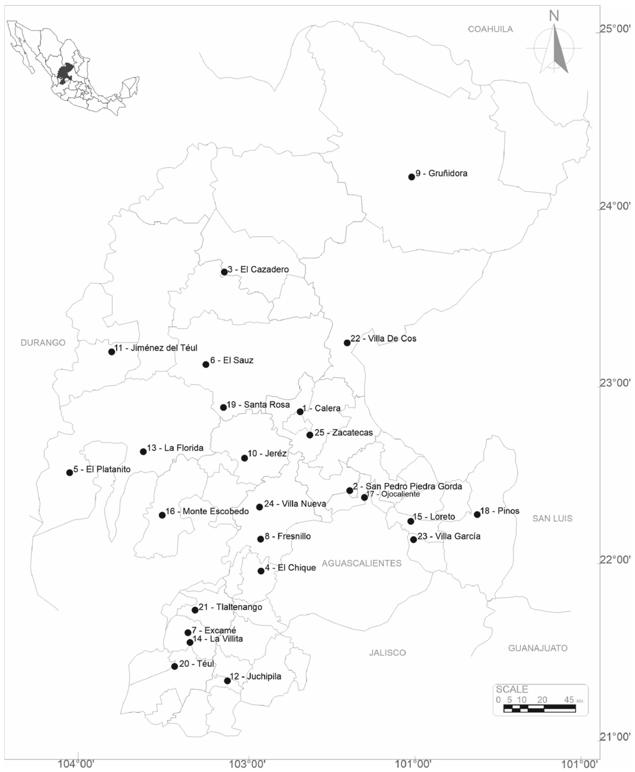
Figure 1. Weather stations in study region of Zacatecas state within the Mexican territory.
Atmosphere 15 00912 g001
Figure 2. Architecture of an LSTM model, including the forget gate, input gate, candidate activation, cell state update, and output gate.
Atmosphere 15 00912 g002
Figure 3. N-HiTS architecture, including inputs (model, stack and block) and outputs (global forecast, stack residual, forecast, and backstack). Reproduced with permission from Max Mergenthaler-Canseco [19]. Proceedings of the AAAI Conference on Artificial Intelligence; published by Association for the Advancement of Artificial Intelligence, 2023.
Atmosphere 15 00912 g003
Figure 4. Hierarchical structure of interpolation granularity of N-HiTS architecture. Reproduced with permission from Max Mergenthaler-Canseco [19]. Proceedings of the AAAI Conference on Artificial Intelligence; published by Association for the Advancement of Artificial Intelligence, 2023.
Atmosphere 15 00912 g004
Figure 5. The observed and forecasted regional SPI time series for the Zacatecas state territory, plotted over the period 1964–2020.
Atmosphere 15 00912 g005
Figure 6. Taylor diagrams by region of observed (SPIo) or reference versus predicted (Tested) SPI values using LSTM and N-HiTS models for the Zacatecas state territory, during the period 1964–2018.
Atmosphere 15 00912 g006
Figure 7. Scatter plots of observed versus predicted regional SPI time series for the Zacatecas state territory, plotted during the period 1964–2018.
Atmosphere 15 00912 g007
Table 1. Categories of standardized precipitation index drought values.
SPI ValueClass
≥2.0Extremely wet
1.5 to 1.99Severely wet
1.0 to 1.49Moderately wet
−0.99 to 0.99Near normal
−1.49 to −0.99Moderately dry
−1.99 to −1.49Severely dry
≤2.0Extremely dry
Table 2. Comparison of metrics of the neural forecasting models’ performance in the validation phase for regional SPI time series for the Zacatecas state, Mexico. Key metrics: Mean Square Error (MSE) and Mean Absolute Error (MAE). The best results are in bold.
LSTMN-HiTS
RegionMSEMAEMSEMAE
Semi-Arid0.49180.58610.32640.4849
High plain0.17230.31170.04550.1696
Mountains1.67111.20160.54720.6661
Canyons0.64560.76390.44330.5769
Table 3. Comparison of neural forecasting models´ performance in training and validation phases for regional SPI time series for the Zacatecas state, Mexico. Key metrics: Determination coefficient (R2) and correlation coefficient (ξ). Bold values represent the best results.
RegionR2ξ
LSTMN-HiTSLSTMN-HiTS
Semi-Arid0.12060.91620.59250.9222
High plain0.54090.95130.70790.9316
Mountains0.25570.96840.59990.9368
Canyons0.61630.96680.66590.9293
Table 4. The probability under normal distribution of prediction error (PE) for N-HiTS models, comparing observed SPI values (SPIo) and predicted SPI values (SPIp) from 1964 to 2018, for regional SPI time series in the state of Zacatecas, Mexico.
RegionPE < 0PE > 0
Semi-Arid0.42410.5759
High plain0.55400.4460
Mountains0.56360.4364
Canyons0.51980.4802
Disclaimer/Publisher’s Note: The statements, opinions and data contained in all publications are solely those of the individual author(s) and contributor(s) and not of MDPI and/or the editor(s). MDPI and/or the editor(s) disclaim responsibility for any injury to people or property resulting from any ideas, methods, instructions or products referred to in the content.