
Vegetation Identification in Hyperspectral Images Using Distance/Correlation Metrics


Abstract
1. Introduction
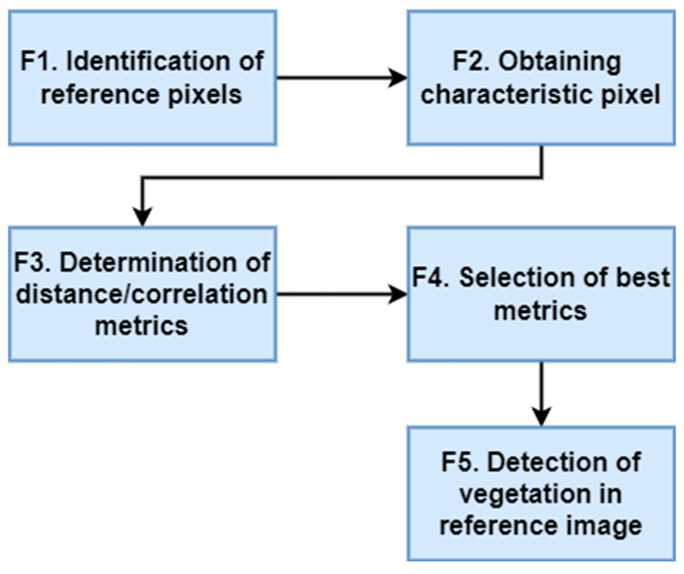
2. Methodology
3. Results and Discussion
4. Conclusions
Author Contributions
Funding
Institutional Review Board Statement
Informed Consent Statement
Data Availability Statement
Acknowledgments
Conflicts of Interest
References
- Pérez-Cabello, F.; Montorio, R.; Alves, D.B. Remote sensing techniques to assess post-fire vegetation recovery. Curr. Opin. Environ. Sci. Health 2021, 21, 100251. [Google Scholar] [CrossRef]
- Andreatta, D.; Gianelle, D.; Scotton, M.; Dalponte, M. Estimating grassland vegetation cover with remote sensing: A comparison between Landsat-8, Sentinel-2 and PlanetScope imagery. Ecol. Indic. 2022, 141, 109102. [Google Scholar] [CrossRef]
- Sripada, R.P. Determining In-Season Nitrogen Requirements for Corn Using Aerial Color-Infrared Photography; North Carolina State University: Raleigh, NC, USA, 2005. [Google Scholar]
- Shikwambana, L.; Xongo, K.; Mashalane, M.; Mhangara, P. Climatic and Vegetation Response Patterns over South Africa during the 2010/2011 and 2015/2016 Strong ENSO Phases. Atmosphere 2023, 14, 416. [Google Scholar] [CrossRef]
- García-Pardo, K.A.; Moreno-Rangel, D.; Domínguez-Amarillo, S.; García-Chávez, J.R. Remote sensing for the assessment of ecosystem services provided by urban vegetation: A review of the methods applied. Urban For. Urban Green. 2022, 74, 127636. [Google Scholar] [CrossRef]
- Neinavaz, E.; Schlerf, M.; Darvishzadeh, R.; Gerhards, M.; Skidmore, A.K. Thermal infrared remote sensing of vegetation: Current status and perspectives. Int. J. Appl. Earth Obs. Geoinf. 2021, 102, 102415. [Google Scholar] [CrossRef]
- Meusburger, K.; Bänninger, D.; Alewell, C. Estimating vegetation parameter for soil erosion assessment in an alpine catchment by means of QuickBird imagery. Int. J. Appl. Earth Obs. Geoinf. 2010, 12, 201–207. [Google Scholar] [CrossRef]
- Henrich, V.; Krauss, G.; Götze, C.; Sandow, C. Index DataBase. A Database for Remote Sensing Indices. 2012. Available online: https://www.indexdatabase.de/db/s-single.php?id=9 (accessed on 29 September 2022).
- Huang, S.; Tang, L.; Hupy, J.P.; Wang, Y.; Shao, G. A commentary review on the use of normalized difference vegetation index (NDVI) in the era of popular remote sensing. J. For. Res. 2021, 32, 1–6. [Google Scholar] [CrossRef]
- Hernández, D.H.B. Aplicación de Índices de Vegetación para Evaluar Procesos de Restauración Ecológica en el Parque Forestal Embalse del Neusa; Universidad Militar Nueva Granada: Neusa, Colombia, 2017. [Google Scholar]
- Gil, L.K.T.; Martínez, D.V.; Saba, M. The Widespread Use of Remote Sensing in Asbestos, Vegetation, Oil and Gas, and Geology Applications. Atmosphere 2023, 14, 172. [Google Scholar] [CrossRef]
- Birth, G.S.; McVey, G.R. Measuring the Color of Growing Turf with a Reflectance Spectrophotometer. Agron. J. 1968, 60, 640–643. [Google Scholar] [CrossRef]
- Wolf, A.F. Using WorldView-2 Vis-NIR multispectral imagery to support land mapping and feature extraction using normalized difference index ratios. In Proceedings of the Algorithms and Technologies for Multispectral, Hyperspectral, and Ultraspectral Imagery XVIII, SPIE Defense, Security, and Sensing, Baltimore, MD, USA, 23–27 April 2012; Volume 8390, pp. 188–195. [Google Scholar] [CrossRef]
- Rouse, J.W., Jr.; Haas, R.H.; Schell, J.A.; Deering, D.W. Monitoring Vegetation Systems in the Great Plains with Erts; Nasa Special Publication; NASA: Washington, DC, USA, 1974. [Google Scholar]
- Kauth, R.J.; Thomas, G.S.P. The tasselled cap—A graphic description of the spectral-temporal development of agricultural crops as seen by Landsat. In Proceedings of the Symposium on Machine Processing of Remotely Sensed Data, West Lafayette, IN, USA, 29 June–1 July 1976. [Google Scholar]
- Tucker, C.J. Red and photographic infrared linear combinations for monitoring vegetation. Remote Sens. Environ. 1979, 8, 127–150. [Google Scholar] [CrossRef]
- Huete, A.R. A soil-adjusted vegetation index (SAVI). Remote Sens. Environ. 1988, 25, 295–309. [Google Scholar] [CrossRef]
- Crippen, R.E. Calculating the vegetation index faster. Remote Sens. Environ. 1990, 34, 71–73. [Google Scholar] [CrossRef]
- Gitelson, A.A.; Merzlyak, M.N. Remote sensing of chlorophyll concentration in higher plant leaves. Adv. Sp. Res. 1998, 22, 689–692. [Google Scholar] [CrossRef]
- Bannari, A.; Asalhi, H.; Teillet, P.M. Transformed difference vegetation index (TDVI) for vegetation cover mapping. In Proceedings of the IEEE International Geoscience and Remote Sensing Symposium, Toronto, ON, Canada, 24–28 June 2002; Volume 5, pp. 3053–3055. [Google Scholar] [CrossRef]
- MaxMax. Enhanced Normalized Difference Vegetation Index (ENDVI). 2015. Available online: https://www.maxmax.com/endvi.htm (accessed on 26 September 2022).
- Adão, T.; Hruška, J.; Pádua, L.; Bessa, J.; Peres, E.; Morais, R.; Sousa, J.J. Hyperspectral Imaging: A Review on UAV-Based Sensors, Data Processing and Applications for Agriculture and Forestry. Remote Sens. 2017, 9, 1110. [Google Scholar] [CrossRef]
- Wan, L.; Li, H.; Li, C.; Wang, A.; Yang, Y.; Wang, P. Hyperspectral Sensing of Plant Diseases: Principle and Methods. Agronomy 2022, 12, 1451. [Google Scholar] [CrossRef]
- Wang, S.; Guan, K.; Zhang, C.; Jiang, C.; Zhou, Q.; Li, K.; Qin, Z.; Ainsworth, E.A.; He, J.; Wu, J.; et al. Airborne hyperspectral imaging of cover crops through radiative transfer process-guided machine learning. Remote Sens. Environ. 2023, 285, 113386. [Google Scholar] [CrossRef]
- Khan, A.; Vibhute, A.D.; Mali, S.; Patil, C.H. A systematic review on hyperspectral imaging technology with a machine and deep learning methodology for agricultural applications. Ecol. Inform. 2022, 69, 101678. [Google Scholar] [CrossRef]
- Chen, D.; Zhang, F.; Tan, M.L.; Chan, N.W.; Shi, J.; Liu, C.; Wang, W. Improved Na+ estimation from hyperspectral data of saline vegetation by machine learning. Comput. Electron. Agric. 2022, 196, 106862. [Google Scholar] [CrossRef]
- Gakhar, S.; Tiwari, K.C. Spectral–Spatial urban target detection for hyperspectral remote sensing data using artificial neural network. Egypt. J. Remote Sens. Sp. Sci. 2021, 24, 173–180. [Google Scholar] [CrossRef]
- Ma, B.; Zeng, W.; Hu, G.; Cao, R.; Cui, D.; Zhang, T. Normalized difference vegetation index prediction based on the delta downscaling method and back-propagation artificial neural network under climate change in the Sanjiangyuan region, China. Ecol. Inform. 2022, 72, 101883. [Google Scholar] [CrossRef]
- Trombetti, M.; Riaño, D.; Rubio, M.A.; Cheng, Y.B.; Ustin, S.L. Multi-temporal vegetation canopy water content retrieval and interpretation using artificial neural networks for the continental USA. Remote Sens. Environ. 2008, 112, 203–215. [Google Scholar] [CrossRef]
- Davies, B.F.R.; Gernez, P.; Geraud, A.; Oiry, S.; Rosa, P.; Zoffoli, M.L.; Barillé, L. Multi- and hyperspectral classification of soft-bottom intertidal vegetation using a spectral library for coastal biodiversity remote sensing. Remote Sens. Environ. 2023, 290, 113554. [Google Scholar] [CrossRef]
- Badola, A.; Panda, S.K.; Roberts, D.A.; Waigl, C.F.; Jandt, R.R.; Bhatt, U.S. A novel method to simulate AVIRIS-NG hyperspectral image from Sentinel-2 image for improved vegetation/wildfire fuel mapping, boreal Alaska. Int. J. Appl. Earth Obs. Geoinf. 2022, 112, 102891. [Google Scholar] [CrossRef]
- Rumpf, T.; Mahlein, A.-K.; Steiner, U.; Oerke, E.-C.; Dehne, H.-W.; Plümer, L. Early detection and classification of plant diseases with Support Vector Machines based on hyperspectral reflectance. Comput. Electron. Agric. 2010, 74, 91–99. [Google Scholar] [CrossRef]
- Wang, L.; Wang, Q. Fast spatial-spectral random forests for thick cloud removal of hyperspectral images. Int. J. Appl. Earth Obs. Geoinf. 2022, 112, 102916. [Google Scholar] [CrossRef]
- Ding, X.; Wang, Q.; Tong, X. Integrating 250 m MODIS data in spectral unmixing for 500 m fractional vegetation cover estimation. Int. J. Appl. Earth Obs. Geoinf. 2022, 111, 102860. [Google Scholar] [CrossRef]
- Shore, S.N. Astrochemistry. In Encyclopedia of Physical Science and Technology; Academic Press: Cambridge, MA, USA, 2003; pp. 665–678. [Google Scholar] [CrossRef]
- Galle, N.J.; Brinton, W.; Vos, R.; Basu, B.; Duarte, F.; Collier, M.; Ratti, C.; Pilla, F. Correlation of WorldView-3 spectral vegetation indices and soil health indicators of individual urban trees with exceptions to topsoil disturbance. City Environ. Interact. 2021, 11, 100068. [Google Scholar] [CrossRef]
- Thorp, K.R.; French, A.N.; Rango, A. Effect of image spatial and spectral characteristics on mapping semi-arid rangeland vegetation using multiple endmember spectral mixture analysis (MESMA). Remote Sens. Environ. 2013, 132, 120–130. [Google Scholar] [CrossRef]
- Zhu, Y.; Zhang, Y.; Zheng, Z.; Liu, Y.; Wang, Z.; Cong, N.; Zu, J.; Tang, Z.; Zhao, G.; Gao, J.; et al. Converted vegetation type regulates the vegetation greening effects on land surface albedo in arid regions of China. Agric. For. Meteorol. 2022, 324, 109119. [Google Scholar] [CrossRef]
- Smyth, T.A.G.; Wilson, R.; Rooney, P.; Yates, K.L. Extent, accuracy and repeatability of bare sand and vegetation cover in dunes mapped from aerial imagery is highly variable. Aeolian Res. 2022, 56, 100799. [Google Scholar] [CrossRef]
- Tian, J.; Zhang, Z.; Philpot, W.D.; Tian, Q.; Zhan, W.; Xi, Y.; Wang, X.; Zhu, C. Simultaneous estimation of fractional cover of photosynthetic and non-photosynthetic vegetation using visible-near infrared satellite imagery. Remote Sens. Environ. 2023, 290, 113549. [Google Scholar] [CrossRef]
- Lyons, R. Distance covariance in metric spaces. Ann. Probab. 2013, 41, 3284–3305. [Google Scholar] [CrossRef]
- Székely, G.J.; Rizzo, M.L. Brownian distance covariance. Ann. Appl. Stat. 2009, 3, 1236–1265. [Google Scholar] [CrossRef]
- Connor, R. A tale of four metrics. In International Conference on Similarity Search and Applications—SISAP 2016; Lecture Notes in Computer Science; Springer: Cham, Switzerland, 2016; Volume 9939, pp. 210–217. [Google Scholar] [CrossRef]
- Bray, J.R.; Curtis, J.T. An Ordination of the Upland Forest Communities of Southern Wisconsin. Source Ecol. Monogr. 1957, 27, 325–349. [Google Scholar] [CrossRef]
- Novotn, V.T. Implementation notes for the soft cosine measure. In Proceedings of the CIKM ’18: 27th ACM International Conference on Information and Knowledge Management, Torino, Italy, 22–26 October 2018; pp. 1639–1642. [Google Scholar] [CrossRef]
- Curcio, A.C.; Barbero, L.; Peralta, G. UAV-Hyperspectral Imaging to Estimate Species Distribution in Salt Marshes: A Case Study in the Cadiz Bay (SW Spain). Remote Sens. 2023, 15, 1419. [Google Scholar] [CrossRef]
- ESRI. ENVI 2023. 2023. Available online: https://www.esri.com/partners/l3harris-technologie-a2T39000001dNCnEAM/envi-a2d5x000005jPrfAAE (accessed on 28 June 2023).
- Duarte, L.; Teodoro, A.C.; Monteiro, A.T.; Cunha, M.; Gonçalves, H. QPhenoMetrics: An open source software application to assess vegetation phenology metrics. Comput. Electron. Agric. 2018, 148, 82–94. [Google Scholar] [CrossRef]
- Zhang, Y.; Wang, Y.; Ding, N. Spatial Effects of Landscape Patterns of Urban Patches with Different Vegetation Fractions on Urban Thermal Environment. Remote Sens. 2022, 14, 5684. [Google Scholar] [CrossRef]


Disclaimer/Publisher’s Note: The statements, opinions and data contained in all publications are solely those of the individual author(s) and contributor(s) and not of MDPI and/or the editor(s). MDPI and/or the editor(s) disclaim responsibility for any injury to people or property resulting from any ideas, methods, instructions or products referred to in the content. |
© 2023 by the authors. Licensee MDPI, Basel, Switzerland. This article is an open access article distributed under the terms and conditions of the Creative Commons Attribution (CC BY) license (https://creativecommons.org/licenses/by/4.0/).
Share and Cite
Chanchí Golondrino, G.E.; Ospina Alarcón, M.A.; Saba, M. Vegetation Identification in Hyperspectral Images Using Distance/Correlation Metrics. Atmosphere 2023, 14, 1148. https://doi.org/10.3390/atmos14071148
Chanchí Golondrino GE, Ospina Alarcón MA, Saba M. Vegetation Identification in Hyperspectral Images Using Distance/Correlation Metrics. Atmosphere. 2023; 14(7):1148. https://doi.org/10.3390/atmos14071148
Chicago/Turabian StyleChanchí Golondrino, Gabriel E., Manuel A. Ospina Alarcón, and Manuel Saba. 2023. "Vegetation Identification in Hyperspectral Images Using Distance/Correlation Metrics" Atmosphere 14, no. 7: 1148. https://doi.org/10.3390/atmos14071148
APA StyleChanchí Golondrino, G. E., Ospina Alarcón, M. A., & Saba, M. (2023). Vegetation Identification in Hyperspectral Images Using Distance/Correlation Metrics. Atmosphere, 14(7), 1148. https://doi.org/10.3390/atmos14071148