Article

Construction and Research of Ultra-Short Term Prediction Model of Solar Short Wave Irradiance Suitable for Qinghai–Tibet Plateau

1
School of Ecology and Environment, Tibet University, Lhasa 850032, China
2
College of Science, Fuyang Preschool Education College, Fuyang 236015, China
3
Binary Graduate School, Binary University of Management & Entrepreneurship, Puchong 47100, Malaysia
*
Author to whom correspondence should be addressed.
Atmosphere 2023, 14(7), 1150; https://doi.org/10.3390/atmos14071150
Submission received: 24 June 2023 / Revised: 9 July 2023 / Accepted: 11 July 2023 / Published: 14 July 2023

Abstract

:
The Qinghai–Tibet Plateau region has abundant solar energy, which presents enormous potential for the development of solar power generation. Accurate prediction of solar radiation is crucial for the safe and cost-effective operation of the power grid. Therefore, constructing a suitable ultra-short-term prediction model for the Tibetan Plateau region holds significant importance. This study was based on the autoregressive integrated moving average model (ARIMA), random forest model (RF), and long short-term memory model (LSTM) to construct a prediction model for forecasting the average irradiance for the next 10 min. By locally testing and optimizing the model parameter, the study explored the applicability of each model in different seasons and investigates the impact of factors such as training dataset and prediction time range on model accuracy. The results showed that: (1) the accuracy of the ARIMA model was lower than the persistence model used as a reference model, while both the RF model and LSTM model had higher accuracy than the persistence model; (2) the sample size and distribution of the training dataset significantly affected the accuracy of the models. When both the season (distribution) and sample size were the same, RF achieved the highest accuracy. The optimal sample sizes for ARIMA, RF, and LSTM models in each season were as follows: spring (3564, 1980, 4356), summer (2772, 4752, 2772), autumn (3564, 3564, 4752), and winter (3168, 3168, 4752). (3) The prediction forecast horizon had a significant impact on the model accuracy. As the forecast horizon increased, the errors of all models gradually increased, reaching a peak between 80 and 100 min before slightly decreasing and then continuing to rise. When both the season and forecast horizon were the same, RF had the highest accuracy, with an RMSE lower than ARIMA by 65.6–258.3 W/m2 and lower than LSTM by 3.7–83.3 W/m2. Therefore, machine learning can be used for ultra-short-term forecasting of solar irradiance in the Qinghai–Tibet Plateau region to meet the forecast requirements for solar power generation, providing a reference for similar studies.

1. Introduction

Solar energy, as one of the most promising renewable energy sources [1], is abundant, green, and clean. Solar power generation is bound to experience significant development [2]. The Qinghai–Tibet Plateau region is exceptionally rich in solar energy, with annual sunshine duration ranging from approximately 1500 to 3400 h. The region holds tremendous potential for solar power generation. However, there are significant fluctuations in power generation, and sudden changes in power output can have adverse effects on the stability of the grid [3]. Accurate prediction of solar power generation provides a suitable means for the safe and efficient operation of the grid [4], which is crucial for reducing the impact of integrating solar power systems into the power grid [5]. Therefore, precise forecasting of power generation is of utmost importance. Solar irradiance is a primary determining factor affecting power output [6], making irradiance prediction one of the most challenging focal points currently. Therefore, in the context of China’s dual carbon strategy goals, establishing a suitable solar irradiance prediction model for the Tibetan Plateau holds great significance.
Solar radiation series, as a type of time series, can be predicted using time series analysis methods [7,8], with autoregressive integrated moving average (ARIMA) being widely applied. In the study by Zhang [9], a hybrid model combining ARIMA and artificial neural networks (ANN) was constructed, and the results showed that the model effectively improved prediction accuracy. In the study by Reikard [10], multiple radiation datasets with resolutions of 5, 15, 30, and 60 min were used to build ARIMA models for predicting solar irradiance from the next 5 min to several hours ahead. The ARIMA model with time-varying coefficients (logs) obtained the best results. Ferrari [11] conducted a study on solar irradiance time series and predicted it using AR, ARMA, and ARIMA models. They compared these models with persistence models, k-nearest neighbors models, and support vector machine models. The results indicated that the ARIMA model provided the best fit. In the study by Yang [12], ARIMA models were constructed using different types of meteorological data as input variables to predict solar radiation for the next 1 h. It was found that utilizing cloud information for prediction could improve accuracy. The ARIMA model constructed by Das [13] provided reliable predictions for solar radiation and solar photovoltaic power output. It is flexible enough to incorporate more information and its performance improves with an increasing number of data points.
In recent years, machine learning became one of the main methods for irradiance prediction, with random forest (RF) being widely employed by researchers due to its high performance, low overfitting risk, and fast training speed [14]. In the study by Sun [15], multiple meteorological, solar radiation, and air pollution index data from various stations were utilized to construct an RF model for irradiance prediction. The results demonstrated that the RF model outperformed empirical methods in terms of fitting accuracy. Fouilloy [16] analyzed 11 statistical and machine learning methods used for solar irradiance prediction and compared their performance across three different meteorological stations. For sites with high variability, the reliability of predictions was lower, but RF demonstrated the best predictive performance. In the study by Benali [17], an RF-based radiation prediction model was found to outperform intelligent persistence and artificial neural network models. In the study by Zeng [18], the simulated results of a high-density daily solar radiation network constructed based on the RF model showed good agreement with measured values in China. Hou [19] utilized Himawari-8 AHI data and constructed a prediction model based on random forest (RF) to estimate the downward shortwave radiation at the surface in China. They achieved promising results with this approach. Villegas-Mier [20] proposed a RF-based solar radiation prediction model. The results showed an accuracy improvement of 95.98% compared to traditional linear regression methods, and it exhibited strong robustness.
With the rapid development of deep learning, researchers extended its application to the field of solar radiation prediction, particularly the widespread use of the long short-term memory (LSTM) model due to its strong suitability for time series forecasting. In the study by Srivastava and Lessmann [21], an LSTM-based irradiance prediction model was constructed, validating its robustness and demonstrating that the optimally configured LSTM model outperformed other methods. Qing and Niu [22] utilized two years of radiation data collected in Cape Verde to train and predict using an LSTM model. Their results showed a 18.34% lower RMSE compared to multilayered feedforward neural networks. Wen [23] developed a deep recursive neural network with long short-term memory (DRNN-LSTM) for solar power generation and load forecasting. Their performance surpassed that of multilayer perceptron (MLP) and support vector machine (SVM). Lan Huynh [24] developed an LSTM-based model for radiation prediction in Vietnam, forecasting radiation for 1, 5, 10, 15, and 30 min into the future. Their results indicated superiority over other models. In the study by Huang [25], an LSTM-based irradiance prediction model was developed, analyzing the influence of different lag time parameters, primary inputs, and auxiliary inputs on the model’s predictive performance. The results showed that the accuracy was superior to that of the BPNN model. Sorkun [26] proposed an LSTM-based solar radiation prediction model and investigated the impact of various meteorological variables. The research results demonstrated that the multivariate model outperformed the previous univariate models. Liu [27] conducted solar radiation prediction and evaluation using seven years of radiation data from the U.S. Department of Energy’s Atmospheric Radiation Measurement (ARM) center. Their results demonstrated that LSTM had the best overall performance, outperforming XGBoost and ARIMA models. Gao [28] developed a deep generative model based on LSTM for multi-step solar irradiance prediction. The results showed that the model effectively avoids the issue of error accumulation. Compared to the traditional regression LSTM model, it achieved an accuracy improvement of 7.7%. Bou-Rabee [29] proposed a solar radiation prediction model based on attention mechanism and bidirectional long short-term memory (BiLSTM). The model was designed separately for sunny and cloudy weather conditions. The results showed that its performance was superior to other deep learning networks. Alizamir [30] constructed multiple solar radiation prediction models, and the results indicated that the combination of LSTM model and wavelet transform technique can enhance the accuracy of radiation prediction based on climatic parameters.
The Qinghai–Tibet Plateau region has abundant solar energy resources. In the context of China’s dual-carbon strategy goals, it is of great significance to establish a solar shortwave radiation prediction model suitable for this region. Previous studies showed that using statistical models, machine learning, and deep learning to establish solar radiation prediction models is an advanced and effective research approach. However, based on the radiation characteristics of different regions, it is necessary to perform local testing and optimization of model parameters. Therefore, in this study, utilizing ground solar shortwave radiation flux observation data, representative methods including ARIMA, RF, and LSTM algorithms were employed to construct models for predicting the average solar shortwave radiation for the next 10 min. Sensitivity testing and optimization of key parameters were conducted, and a comparative analysis was carried out to reveal the advantages and limitations of these methods in irradiance prediction, aiming to establish a radiation prediction model suitable for the Qinghai–Tibet Plateau region. These data-driven prediction methods heavily rely on the training dataset [15], and the sample size of the training set is a determining factor for the model’s generalization ability [31]. The sample size affects the learning and training effectiveness of the model, and the accuracy of the model can also be influenced by the numerical distribution of the training set [32], which is influenced by seasonal variations in irradiance. Therefore, it is necessary to conduct research by classifying seasons when predicting irradiance. However, there is limited research on the impact of factors such as sample size and numerical distribution of the training set on the prediction accuracy of the model, highlighting the need for relevant studies. Additionally, the prediction forecast horizon has a significant impact on the model’s accuracy, and a quantitative study on the accurate prediction forecast horizon of each model in different seasons can provide reference for the construction of prediction models in this region.
The structure of this paper is as follows: In Section 2, the research area, data preprocessing, dataset configuration, and data features are introduced. In Section 3, the research methods are presented, including the principles and construction of the ARIMA, RF, and LSTM models. In Section 4 and Section 5, the experimental results are showcased and discussed.

2. Data

Constructing a solar radiation prediction model requires data-driven approaches and validation. Analyzing the differences in the training set and the impact of the prediction time range on model accuracy necessitates an examination of the data’s characteristics.

2.1. Overview of the Study Area

Yangbajing (90°33′ E,30°05′ N) is located 90 km northwest of Lhasa, Tibet. It has an average elevation of 4300 m and features a flat terrain surrounded by mountains. The area experiences short spring and autumn seasons, with warm and humid summers and long, cold winters. It enjoys abundant sunshine throughout the year, with an annual sunshine duration of over 2800 h. A solar photovoltaic power station was built in this area. The Yangbajing Atmospheric Observatory, operated by the Institute of Atmospheric Physics, Chinese Academy of Sciences, conducted comprehensive atmospheric observations since 2018. The observatory covers a wide range of detection wavelengths, from ultraviolet to infrared, terahertz, and millimeter waves. It enables high vertical resolution (10–100 m), high temporal resolution (1 min to 1 h), and continuous simultaneous quantitative measurements of multiple atmospheric variables throughout the entire atmospheric column.

2.2. Data Sources

This study focused on the analysis of shortwave solar radiation data obtained from the four-component radiometer MR-60 at the Yangbajing Atmospheric Observatory. The spectral range of the data was 285–3000 nm, and the unit was W/m2. The data were sampled at a frequency of 1 min. A total of 366 days of data, from 1 June 2019 to 31 May 2020, were selected for analysis. Samples with zero radiation during the nighttime were excluded [33], and only data collected between 8:00 and 19:00 during the day were retained. The data were then resampled to calculate the average radiation values over 10 min intervals. Thus, there were 66 samples per day.
Since the accuracy of the models can be influenced by the distribution of the dataset, the distribution of radiation data is related to seasonal variations. Therefore, in this experiment, the data were divided into four datasets based on seasons: spring (March–May), summer (June–August), autumn (September–November), and winter (December–February). Each season had a similar number of samples. The training and testing datasets were split in a 6:1 ratio, and the models were trained to predict the 10 min average radiation for different seasons. This study used historical time series data of solar radiation as input variables for the models. By conducting sensitivity experiments to determine the optimal parameters of each model, the study performed training, prediction, and evaluation to develop short-term radiation prediction models suitable for different seasons in the Qinghai–Tibet Plateau region.

2.3. Data Characteristics

Different datasets require testing and optimization of model parameters based on their respective data characteristics. Previous research results showed significant seasonal variations in solar irradiance, and so, it is important to understand the seasonal characteristics of the dataset. Since only daytime data were retained, the training dataset consisted of multiple samples from different quantities of daytime periods, necessitating analysis of this time period. Additionally, understanding the diurnal variations in the data helps determine the input features of the model.

2.3.1. Seasonal Characteristics

According to Table 1, the solar radiation in the Yangbajing region exhibited significant seasonal variations. The peak occurred in summer, reaching 1713 W/m2, which was much higher than the solar constant. This may be attributed to the influence of clouds [34] and terrain [35]. The standard deviation of radiation was higher in spring and summer, and lower in winter, indicating greater fluctuations in solar radiation during spring and summer, and relatively stable conditions during winter. This can be attributed to the higher rainfall and frequent weather changes in spring and summer, while winter experienced more stable weather conditions.

2.3.2. Diurnal Variation Characteristics

According to Figure 1 and Table 2, the diurnal variations of solar radiation in the Yangbajing region exhibited similar patterns in different seasons, showing a single-peak inverted “U” shape. Due to the rotation of the Earth and the variation of the solar zenith angle, the radiation showed a clear periodic variation with a peak around 11–15 o’clock. The standard deviation of radiation in all four seasons is highest around 14–15 o’clock and lowest at 8 o’clock, indicating greater fluctuation at noon and relatively stable conditions in the morning. Additionally, in spring, autumn, and winter, there were often instances in the morning (8–10 o’clock) and evening (17–18 o’clock) where the instantaneous radiation was much higher than the average value in the low radiation zone.
Based on the comprehensive analysis, it can be concluded that solar radiation exhibits significant variations across different seasons. Therefore, the numerical distribution of the training datasets used by the models will differ greatly among the seasons. Each dataset representing a specific season corresponds to a distinct numerical distribution of the training set. Solar radiation historical data were utilized as input for statistical methods and machine learning models. Ignoring the prominent characteristics of solar radiation would result in suboptimal predictions [36]. Hence, it is necessary to classify the datasets according to the seasonal variations of solar radiation and develop separate prediction models for each season to improve accuracy. Additionally, exploring the impact of the numerical distribution differences in the training sets caused by seasonal factors on model accuracy can also be investigated.

3. Methodology

Each prediction method will be briefly described in this section: persistence model, ARIMA, random forest, and LSTM model. The persistence model is a simple model that is easy to implement and does not require any training steps or historical dataset. It is typically used as a reference model for comparison in terms of accuracy against the other three more complex models.

3.1. Persistence Model

The persistence model, the simplest forecasting model, assumes that the future value is identical to the previous one [17]. The formula is as follows:
y ^ t + h = y t
y ^ t and y t represent the predicted value and the measured value of irradiance at time t, respectively, the h represent the forecast horizon.

3.2. ARIMA Prediction Model

ARIMA is a regression equation that is based on the linear relationship between the future values of a variable and its historical values, as well as the historical values and current value of the random error term. It consists of three components: autoregressive (AR), differencing (I), and moving average (MA), denoted by the parameters p, d, and q, respectively [37]. The ARIMA model can be represented as follows:
X k = φ 1 X k 1 + φ 2 X k 2 + + φ p X k p + ε k θ 1 ε k 1 θ 2 ε k 2 θ q ε k q
φ i (i = 1, 2, …, p) represents the autoregressive coefficients, θ i (i = 1, 2, …, q) represents the moving average coefficients, p and q are the orders of the model, and ε k represents the error term [38]. The modeling steps are as follows: (1) Stationarity Test: Perform a statistical test for unit root, such as the augmented Dickey–Fuller test, on the irradiance time series. If the series fails the test, apply methods like differencing, moving average, or logarithmic transformation to transform it into a stationary series. (2) Test for Pure Randomness: Conduct a test for white noise, such as using the Ljung–Box statistic, on the irradiance time series to assess the presence of serial correlation. (3) Model Identification: Determine the order of the model by estimating the autoregressive order (p) and the moving average order (q) based on the autocorrelation function (ACF) and partial autocorrelation function (PACF) estimates [39]. (4) Parameter Estimation: Use the method of least squares or maximum likelihood estimation to estimate the unknown parameter values in the model. (5) Model Validation: Perform significance tests for the estimated parameters and assess the overall significance of the model. (6) Model Optimization: Optimize the model by comparing the values of information criteria functions such as the Akaike information criterion (AIC), Bayesian information criterion (BIC), Hannan–Quinn information criterion (HQIC), etc. Choose the model with the minimum values of these criteria as the optimal model [24].

3.3. RF Prediction Model

RF (random forest) is an ensemble learning method in machine learning, where each tree is constructed from a random subset of the original data during the training process [40]. A randomly selected set of features is used to fit each tree. The random selection of data and features helps to prevent any correlation between the trees and the results of a large number of trees are averaged to address overfitting issues associated with individual decision trees [41]. The steps for building the RF model are as follows.

3.3.1. Data Transformation and Feature Extraction

Transform the solar irradiance time series data into supervised learning data suitable for machine learning by using a sliding window. Use historical time ranges X t 1 , X t 2 , X t 3 , …, X t m as input variables and use future time ranges X t + 1 , X t + 2 , X t + 3 , …, X t + n as output variables. Reconstruct the data to transform it from one-dimensional to multi-dimensional format. The primary objective is to determine the input feature quantity m, which represents the dimensionality of the input matrix [17]. Split the solar irradiance time series dataset into training, validation, and testing sets. Then, using 1, 2, 3, …, M (m < M) steps of time series data as model input variables and training the model with default parameters on the training set, validate it on the validation set to obtain the optimal input feature quantity m.

3.3.2. Model Optimization

Due to the nature of time series data, cross-validation methods were not used for parameter tuning. In this experiment, the rolling origin prediction method was employed to optimize the model [42]. The steps are as follows: (1) The dataset was redivided into training and test sets in a 6:1 ratio. The first step involved training the models on the training set, followed by predicting and evaluating the test set. (2) The actual value of the first step in the testing set was added back to the training set. (3) With the updated training set, the model was retrained and used to predict the second step of the testing set. (4) This process was repeated for the entire testing set. By continuously updating the prediction origin and training set, multiple prediction errors for the time series were obtained. During this process, a grid search was performed to continuously adjust the hyperparameters, achieving the functionality of cross-validation to ensure model stability and avoid overfitting.

3.4. LSTM Prediction Model

As an improved model of recurrent neural networks (RNN) in deep learning, LSTM not only possesses powerful capabilities to uncover complex nonlinear relationships in neural networks [43], but also addresses the issue of vanishing gradients commonly encountered in traditional RNN training. The LSTM unit consists of input gates, output gates, and forget gates, which enable the LSTM unit to ‘forget’ or ‘remember’ information in the memory [44]. Σ represents the sigmoid activation function, and tanh represents the hyperbolic tangent activation function. The specific computation process from input to output is as follows [21]:
f t = σ W f h t 1 , x t + b f
i t = σ W i h t 1 , x t + b i
o t = σ W o h t 1 , x t + b o
c ¯ t = tanh W c h t 1 , x t + b c
c t = f t c t 1 + i t c t ¯
h t = o t tanh c t
The symbol “·” Represents the dot product operation between two vectors, “+” represents the addition operation between two vectors, W f , W i , W o , and W c , respectively, denote the weight matrices for the forget gate, input gate, output gate and memory unit, b f , b i , b o , and b c , respectively, denote the bias vectors for the forget gate, input gate, output gate, and memory cell. The input data for each gate are the element-wise product of the previous timestep’s output h t 1 and the current timestep’s input x t , represented as the vector [ h t 1 , x t ], with their corresponding weight vectors. f t , i t , and o t represent the outputs of the σ function at time t, while c ¯ t represents the output of the tanh function at time t. The long-term memory c t and the short-term memory h t at time t are passed to the next LSTM unit [24,25].
A more advanced LSTM architecture involves stacking multiple hidden layers, each consisting of multiple LSTM units, which enables the model to go deeper and achieve higher accuracy [45]. However, when the number of hidden layers is too small, the training performance may be suboptimal, but adding a large number of layers significantly increases the number of trainable parameters [46], leading to reduced model generalization and increased errors. Therefore, we adopted a model architecture with two hidden layers. The construction process was as follows: (1) We used the same data transformation method as RF to convert the original one-dimensional time series of solar irradiance into multidimensional data with m-dimensional input variables and n-dimensional output variables. (2) The rolling origin prediction method was used to optimize the model. The LSTM input layer had m-dimensional input vectors, and the output layer was configured with n neurons corresponding to the prediction time range. The maximum number of neurons in the hidden layer was set to 100. A dropout layer was added after the hidden layer, randomly ignoring neurons and their connections [47]. The rectified linear unit (ReLU) activation function was used, and the optimizer was set to adaptive moment estimation (Adam). The maximum training epochs were limited to 100 to reduce the risk of overfitting [10]. The optimal hyperparameters of the model were obtained through grid search by minimizing the root mean squared error (RMSE) on the validation dataset. Deep learning models were randomly initialized with weights, so each set of parameters was run 20 times, and the average of the experimental results was taken as the performance evaluation metric [22,48]. By following the above-mentioned methods, we can effectively avoid overfitting issues, improve model generalization, and enhance model robustness.

3.5. Model Evaluation

The RMSE is more sensitive to significant deviations in model predictions, and when predicting solar radiation based on historical time series data, it often encounters multiple large errors [49]. Therefore, RMSE is more suitable than other metrics for model evaluation. The formula is as follows:
R M S E = 1 N t = 1 N ( y t y ^ t ) 2
y t , y ^ t and y t ¯ represent the measured value, predicted value, and measured average value of irradiance at time t, respectively. N is the number of samples in the data set.

4. Results and Analysis

By utilizing the constructed solar irradiance prediction models, single-step forecasting can be conducted to investigate the impact of training set differences on each model. The RMSE of the persistence model in spring, summer, autumn, and winter were 92.1, 111.2, 77, and 44.5 W/m2, respectively. By comparing (Table 3), it can be observed that across all seasons, the persistence model exhibited higher accuracy than ARIMA. However, the RMSE for the persistence model was significantly larger than that of the RF and LSTM models. Additionally, multiple-step forecasting can be performed to study the influence of the prediction time range on each model, thereby exploring the forecast horizon within which each model can accurately predict.

4.1. Impact of Training Set on Model

Each model selects the data collected over 6–72 days as the training set for fitting and predicting the irradiance for the next 10 min. The study investigated the influence of the numerical distribution and sample size of the training set on the various models.

4.1.1. ARIMA Model

According to Figure 2, when the ARIMA model was trained on training sets of equal sample size, in most cases, the prediction error was highest in the summer, followed by the spring, and lowest in the winter.
When the seasons were the same, meaning the numerical distribution of the training set was similar, the model’s prediction accuracy fluctuated without a clear trend as the sample size of the training set increased from 6 days to 72 days of collected data. The optimal sample size of the training set was determined when the RMSE was minimized. Table 3 reveals that for the ARIMA model, the optimal sample sizes for the training sets in spring, summer, autumn, and winter were 3564 (54 days), 2772 (42 days), 3564 (54 days), and 3168 (48 days), respectively. The corresponding RMSE values were 114.4 W/m2, 138.5 W/m2, 84.6 W/m2, and 68.8 W/m2.
Table 4 shows that the ARIMA model’s optimal values for the autoregressive order (p) and the moving average order (q) when selecting the optimal sample size for the training set were as follows: spring (p = 4, q = 3), summer (p = 3, q = 2), autumn (p = 3, q = 3), and winter (p = 5, q = 8). Based on this, a short-term irradiance forecasting model for the Qinghai–Tibet Plateau region can be constructed using the ARIMA model that is suitable for different seasons.

4.1.2. RF Model

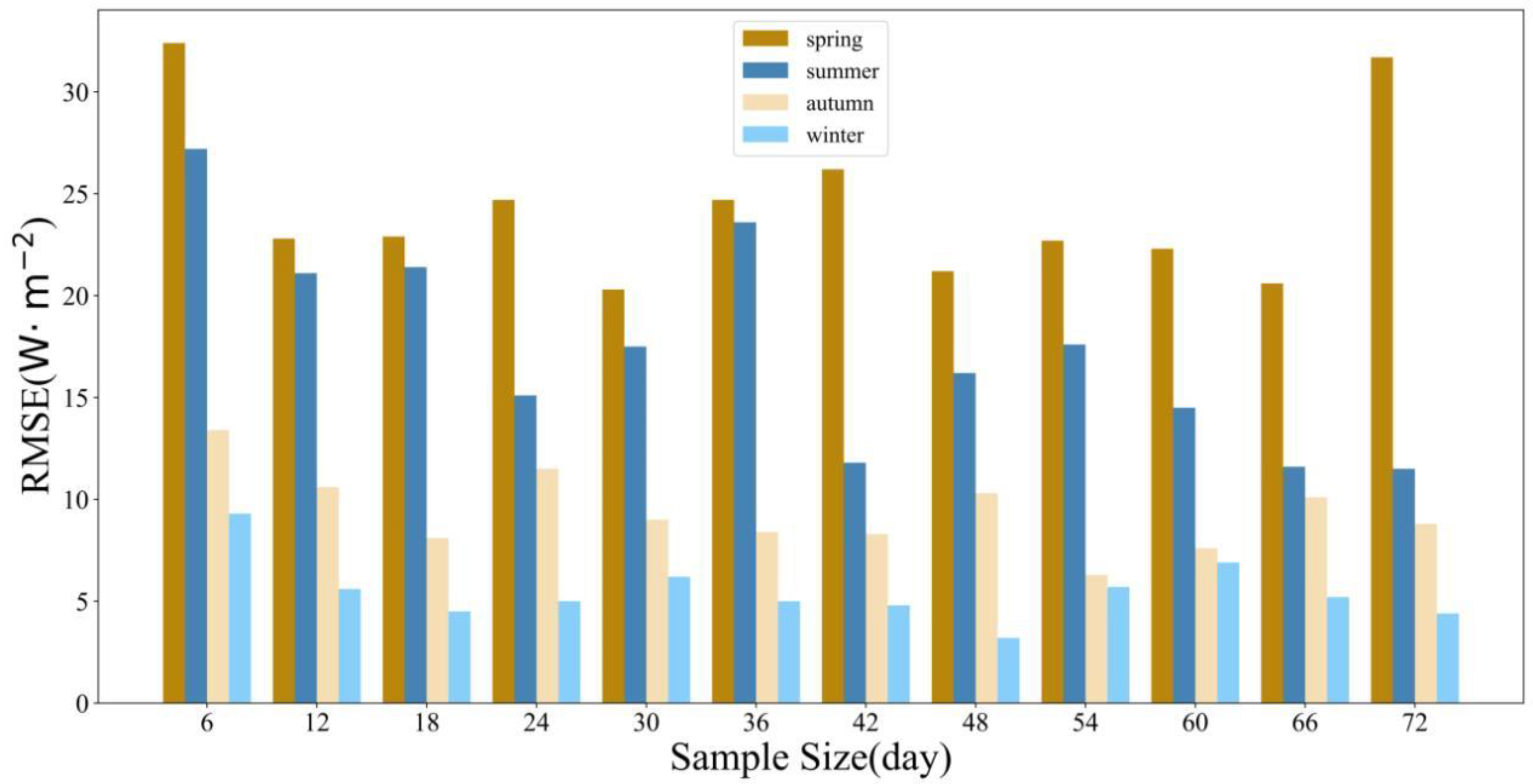
From Figure 3, it can be observed that when the random forest (RF) model was trained on training sets of equal sample size, the prediction error was highest in the spring, followed by the summer, and lowest in the winter.
When the seasons were the same, as the sample size of the training set increased from 6 days to 72 days of collected data, the model’s prediction accuracy fluctuates without a clear trend in all seasons. Table 3 reveals that for the RF model, the optimal sample sizes for the training sets in spring, summer, autumn, and winter were 1980 (30 days), 4752 (72 days), 3564 (54 days), and 3168 (48 days), respectively. The corresponding RMSE values were 20.3 W/m2, 11.5 W/m2, 6.3 W/m2, and 3.2 W/m2.
Table 4 shows that the RF model’s optimal values for the number of trees (estimators) and the maximum depth of trees (max-depth) when training on the optimal sample size of the training set were as follows: spring (estimators = 19, max-depth = 13), summer (estimators = 16, max-depth = 13), autumn (estimators = 25, max-depth = 10), and winter (estimators = 25, max-depth = 14). Based on this, a short-term irradiance forecasting model for different seasons in the Qinghai–Tibet Plateau region can be constructed using the RF model.

4.1.3. LSTM Model

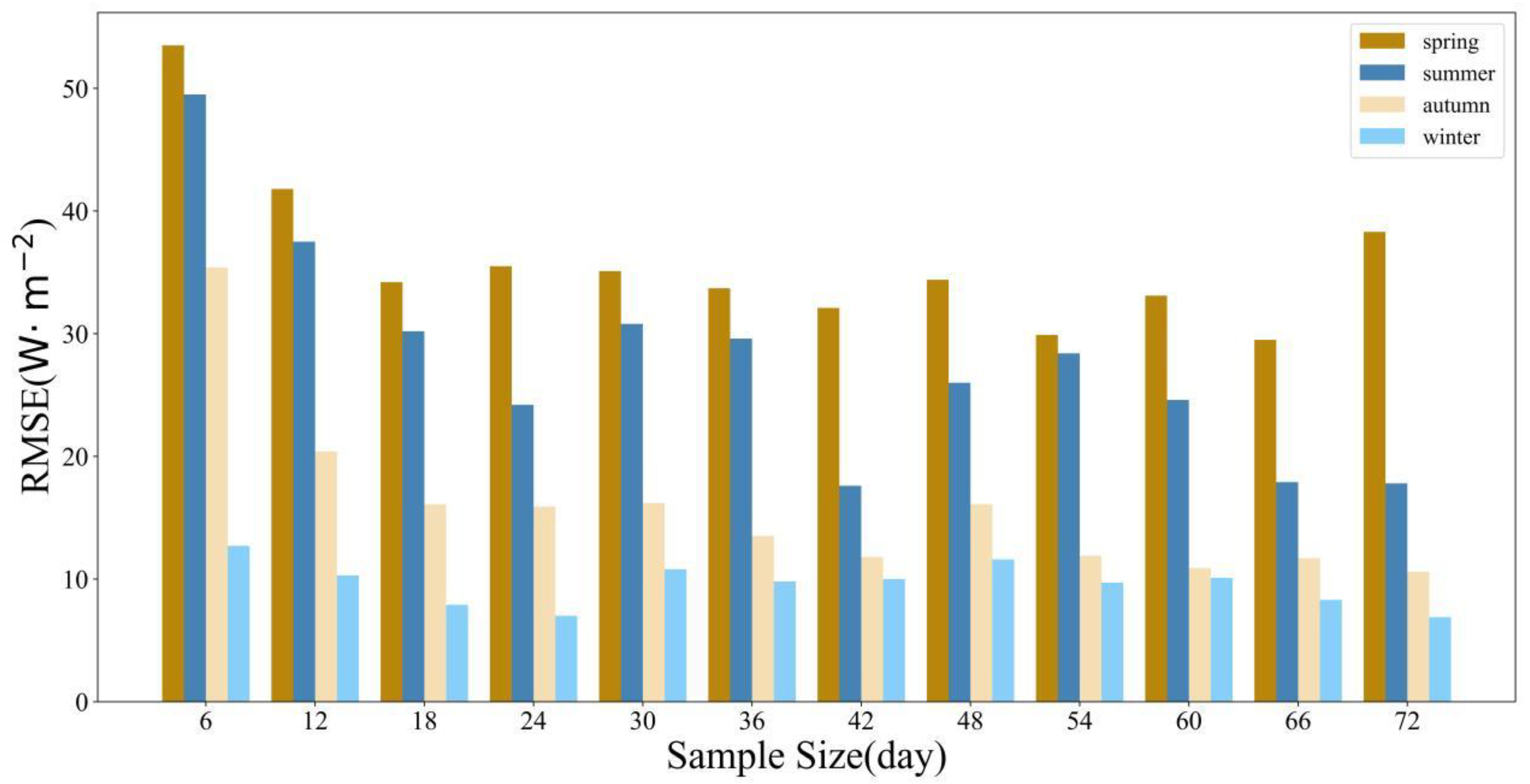
From Figure 4, it can be observed that when the LSTM model was trained on training sets of equal sample size, the prediction error was highest in the spring, followed by the summer, and lowest in the winter.
When the seasons were the same, as the sample size of the training set increased from 6 days to 72 days of collected data, the model’s prediction accuracy for each season fluctuated without a clear trend. Table 3 reveals that for the LSTM model, the optimal sample sizes for the training sets in spring, summer, autumn, and winter are 4356 (66 days), 2772 (42 days), 4752 (72 days), and 4752 (72 days), respectively. The corresponding RMSE values were 29.5 W/m2, 17.6 W/m2, 10.6 W/m2, and 6.9 W/m2.
Table 4 shows that the LSTM model’s optimal values for the number of neurons in each hidden layer when training on the optimal sample size of the training set were as follows: spring (unit1 = 40, unit2 = 60), summer (unit1 = 52, unit2 = 63), autumn (unit1 = 63, unit2 = 67), and winter (unit1 = 40, unit2 = 40). Based on this, a short-term irradiance forecasting model for different seasons in the Qinghai–Tibet Plateau region can be constructed using the LSTM model.

4.1.4. Comparison between Models

According to Table 3, when the sample size was equal, there were significant differences in the accuracy of different models in reflecting the variations in data distribution across different seasons. The ARIMA model exhibited the highest error in the summer and the lowest error in the winter. In contrast, machine learning models such as RF and LSTM showed the highest error in the spring and the lowest error in the winter, which was noticeably different from the statistical model. The model accuracy was greatly influenced by the seasons, which was attributed to the differences in the data distribution of the training sets used for model learning and fitting. The spring and summer solar irradiance exhibited larger standard deviations and greater fluctuations, making predictions more challenging, while the winter solar irradiance had a smaller standard deviation and lower fluctuation, resulting in smaller prediction errors.
From Table 5, it can be observed that when the seasons were the same, i.e., when the data distribution of the training sets was identical, there were significant differences in accuracy among the models at different sample sizes. In the spring, the LSTM model required the largest sample size for training, while the RF model required the smallest. In the summer, the RF model required the largest training set sample size. In the autumn and winter, the LSTM model required the highest sample size. Overall, the LSTM model required a larger sample size for training and fitting [22], while the RF and ARIMA models required relatively smaller sample sizes.
The above results indicate that the accuracy of the models did not necessarily improve with an increase in sample size, as it was also influenced by the data distribution of the training set. The quantity and structure of the training set may have a greater impact on accuracy than the model architecture [50], as model parameters, such as connection weights in neural networks, were estimated from this data [21]. Therefore, it is important to select an appropriate model based on the sample size and data distribution of the training set.
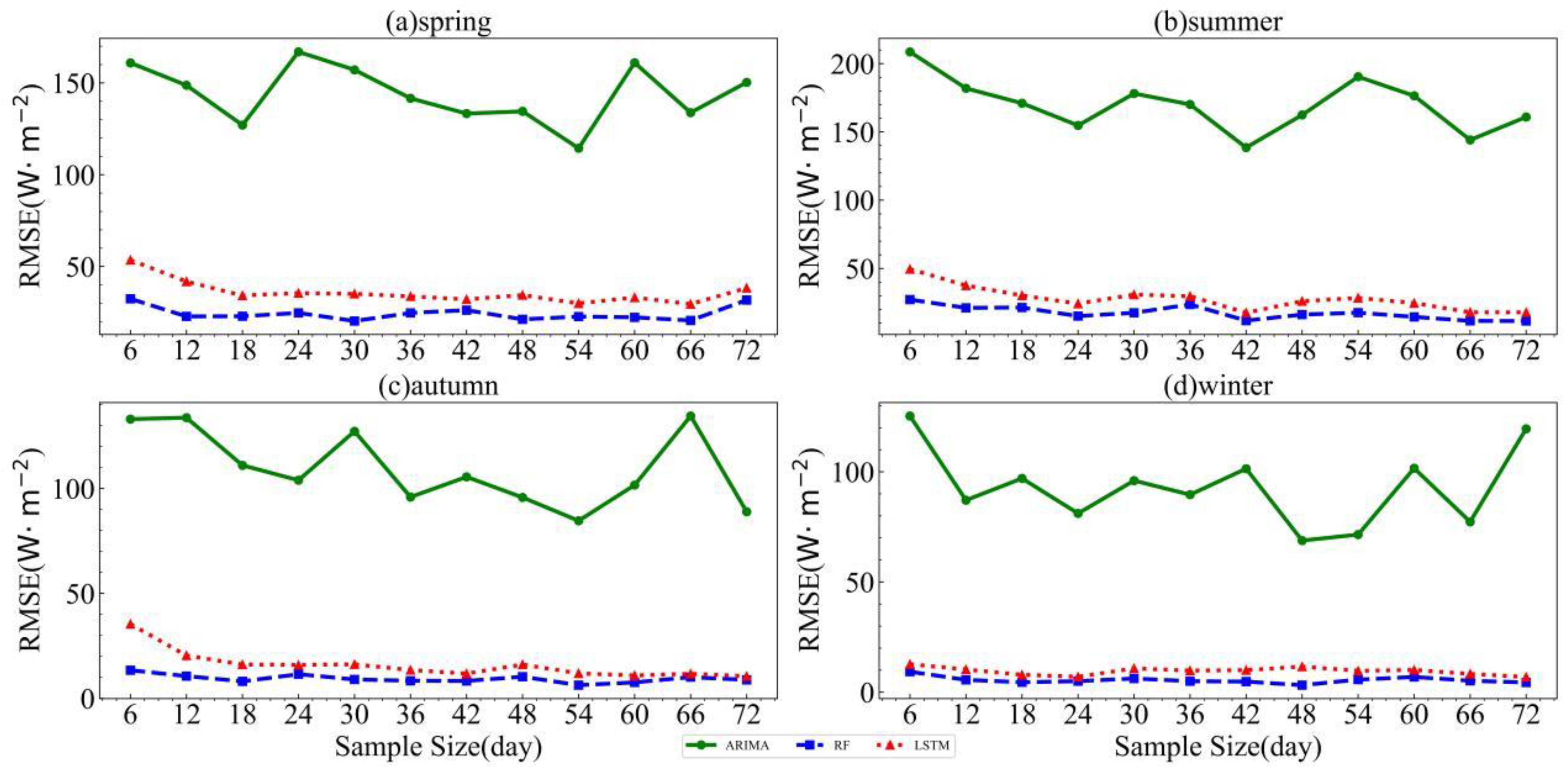
From Figure 5, it can be observed that when each model was trained on the same season and equal sample size training set, regardless of the season, the ARIMA model consistently exhibited the largest prediction error, while the RF model showed the smallest prediction error. The LSTM model’s prediction error was very close to that of the RF model. Time series analysis methods are generally not suitable for short-term forecasting because the prediction error for the next value in a sequence can be large [51]. This may be due to ARIMA neglecting the connections between samples in the training set, while LSTM and RF can leverage all samples for training, resulting in higher information utilization [27]. The output of the ARIMA model depends on a linear combination of historical values, implying that the prediction error is linearly correlated with the historical errors. On the other hand, LSTM and RF can better handle the nonlinear relationships present in the temporal residuals compared to ARIMA [52]. These results indicate that machine learning algorithms are more suitable than ARIMA for short-term forecasting of solar irradiance in the Qinghai–Tibet Plateau region.

4.2. Impact of Forecast Horizon on Model

The optimal training sets and parameters were selected for each model to perform learning and fitting, predicting the 10 min average solar irradiance for the next 2 h. This study investigated the influence of the forecast horizon on the performance of each model. Additionally, a quantitative analysis through multiple-step forecasting will be conducted to explore the time range within which each model can accurately predict.

4.2.1. ARIMA Model

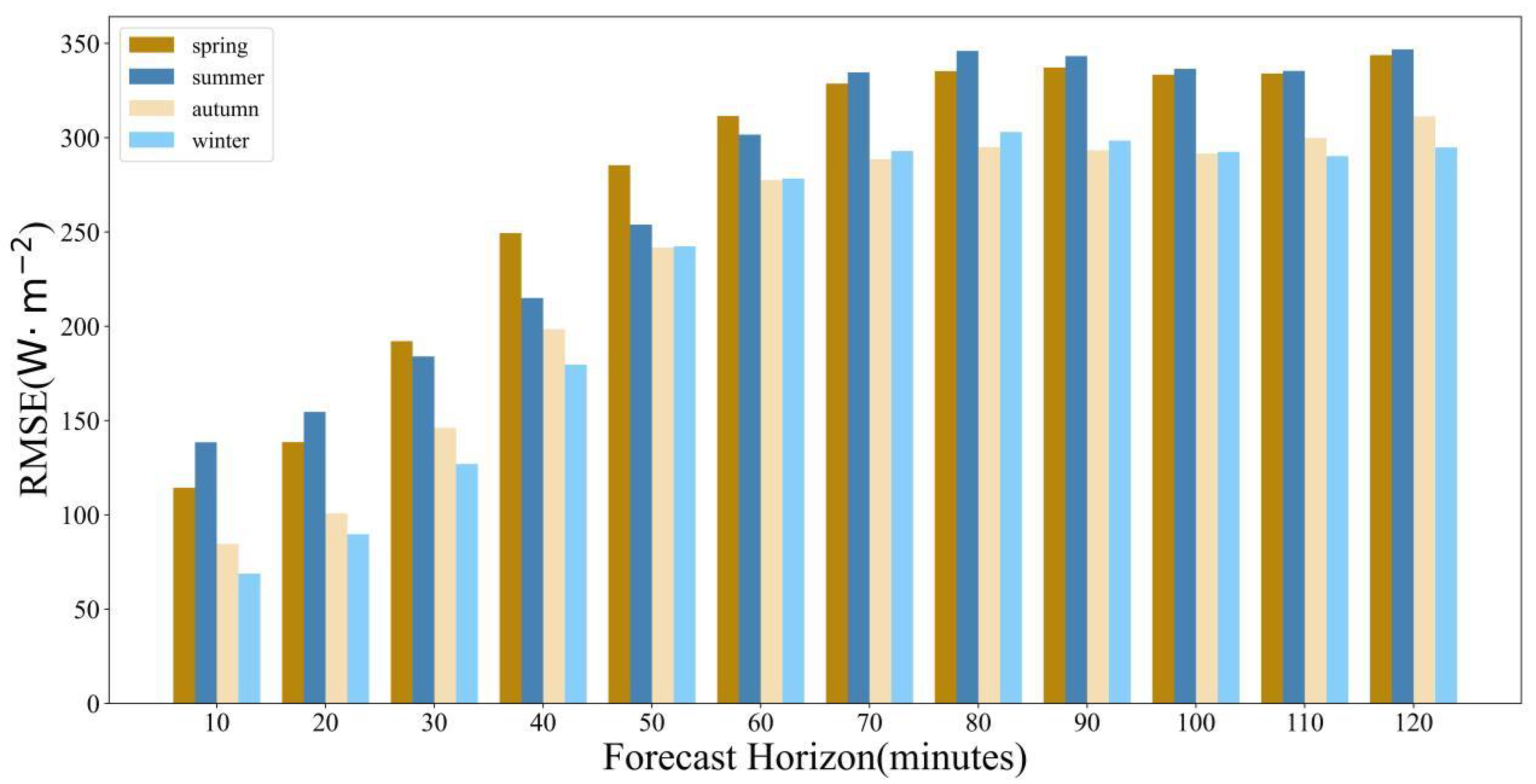
Based on Table 6 and Figure 6, when the forecast horizon was the same, the ARIMA model generally exhibited the largest prediction errors in summer, followed by spring, and the smallest errors in winter. This indicates that the variations in training set data distribution caused by seasonal factors had a significant impact on the model’s accuracy.
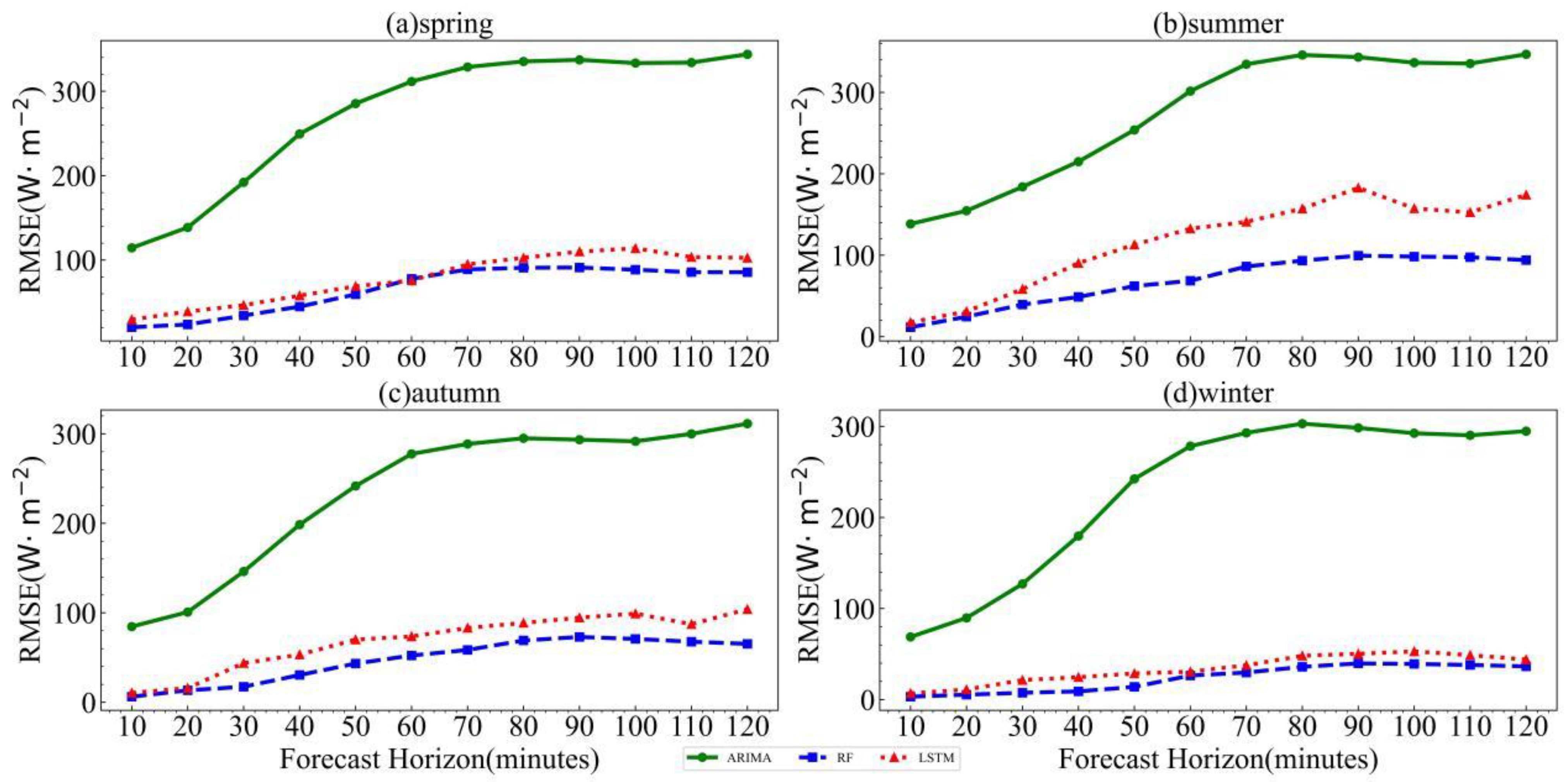
When the seasons were the same, i.e., when the training set data distribution was identical, as the forecast horizon gradually increased from 10 min to 2 h, the ARIMA model’s prediction errors also increased for all seasons, reflecting the accumulation of errors. Within the 10–60 min horizon, the errors of the model in all seasons increased rapidly. After around 70 min, the error trends stabilized gradually. Additionally, the RMSE for each season reached its first peak at 80–90 min (spring: 337.2 W/m2; summer: 346.0 W/m2; autumn: 295.0 W/m2; winter: 303.0 W/m2), followed by a slight decrease before continuing to rise.

4.2.2. RF Model

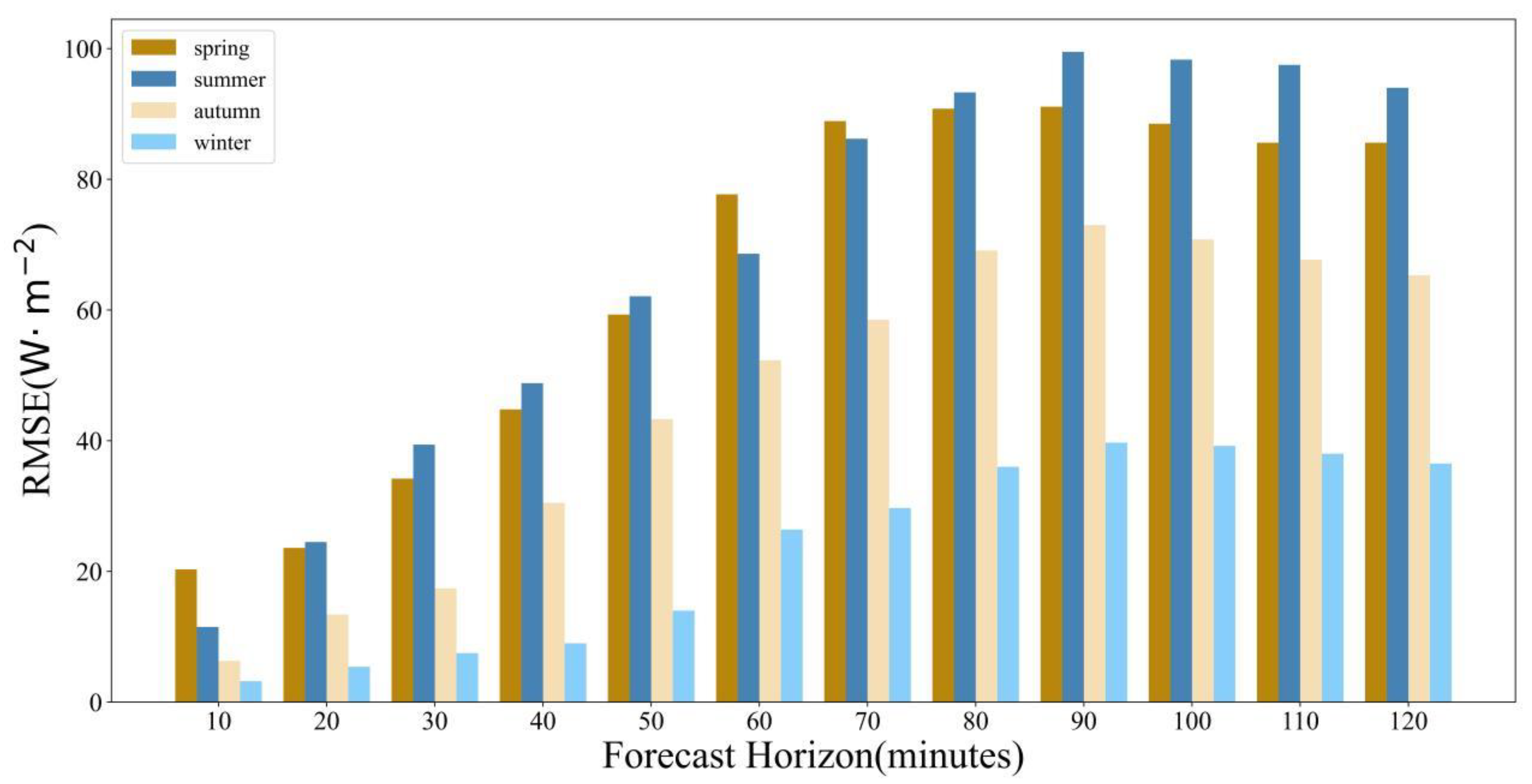
Based on Table 6 and Figure 7, when the forecast horizon was the same, in most cases, the RF model exhibited the largest prediction errors in summer, followed by spring, and the smallest errors in winter.
When the seasons were the same, as the forecast horizon gradually increased from 10 min to 2 h, the RF model’s prediction errors also increased gradually. Within the 10–70 min horizon, the errors of the model in all seasons increased rapidly. After around 80 min, the error trends stabilized gradually. Additionally, the RF model reached a peak RMSE for each season at 90 min (spring: 91.1 W/m2; summer: 99.5 W/m2; autumn: 73.0 W/m2; winter: 39.7 W/m2), followed by a slight decrease.

4.2.3. LSTM Model

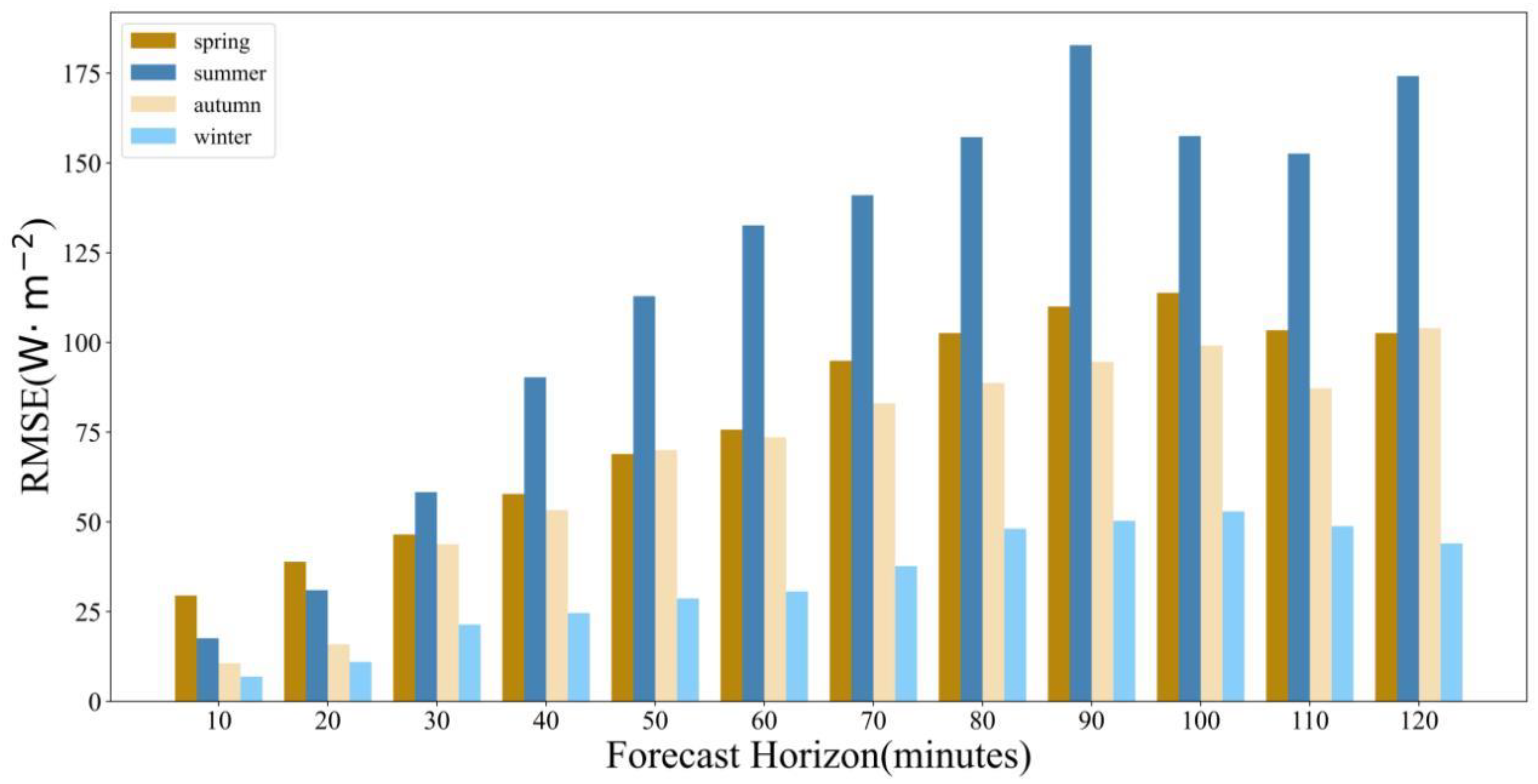
Based on Table 6 and Figure 8, if the forecast horizon was the same, when the horizon was between 10 and 20 min, the LSTM model exhibited the largest prediction errors in spring, followed by summer, and the smallest errors in winter. However, when the forecast horizon exceeded 20 min, the model’s prediction errors were largest in summer, followed by spring, and winter still had the smallest errors.
When the seasons were the same, as the forecast horizon gradually increased from 10 min to 2 h, the LSTM model’s prediction errors also increased gradually. Within the 10–70 min horizon, the errors of the model in all seasons increased rapidly, followed by significant fluctuations. Additionally, the LSTM model reached a peak RMSE for each season at 90–100 min (spring: 113.8 W/m2; summer: 182.8 W/m2; autumn: 99.1 W/m2; winter: 52.9 W/m2), followed by a slight decrease before continuing to rise.

4.2.4. Comparison between Models

From Table 6, it can be observed that when the forecast horizon was the same, there was a significant difference in accuracy among the models for different seasons. However, in most cases, the models exhibited the highest prediction error in summer and the lowest in winter. This was because the training sets used for learning and fitting varied significantly across seasons, with larger variations in solar irradiance during summer, making the prediction more challenging and leading to higher errors. Conversely, during winter, the standard deviation of solar irradiance was smaller, resulting in lower errors.
From Table 6 and Figure 9, it can be observed that when the season was the same, the prediction errors of all models gradually increased as the forecast horizon extended from 10 min to 2 h. This finding was consistent with the conclusion in the literature [53], suggesting that longer forecast horizon lead to a loss of more meteorological information [12]. The sky undergoes significant changes due to factors like clouds [54]. However, after reaching a peak in the horizon of 80–100 min, the errors of the models all experienced a slight decrease.
If the models are evaluated with the same season and the same forecast horizon, regardless of the season, the ARIMA model exhibits the highest prediction error, while the RF model shows the lowest prediction error. The LSTM model’s prediction error is very close to that of the RF model. Although it is possible to improve the accuracy of the LSTM model by increasing the number of hidden layers and neurons, the computational cost is an important consideration in the learning process [24]. Given the higher computational requirements, longer processing time, and larger sample size needed for the LSTM model, the marginal improvement in accuracy does not necessarily demonstrate its superiority, especially when the LSTM model is much more complex than traditional machine learning models [55]. Therefore, the RF model is more suitable for ultra-short-term solar irradiance prediction in the Qinghai–Tibet Plateau region among the selected models.

5. Conclusions

This study first analyzed the radiation characteristics using the monitored shortwave solar radiation data in the Yangbajing area of the Qinghai–Tibet Plateau. Then, prediction models based on ARIMA, RF, and LSTM were constructed to forecast the ultra-short-term solar irradiance at 10 min intervals. The effects of factors such as the sample size and distribution of the training set and the prediction time range on the prediction performance of different models were investigated, leading to the following conclusions:
  • Using the persistence model as a reference model, radiation forecasting was performed based on the ARIMA, RF, and LSTM models. Across all seasons, the accuracy of the ARIMA model was lower than that of the persistence model, but the RF and LSTM models exhibited higher accuracy than the persistence model.
  • The prediction accuracy of the ARIMA, RF, and LSTM models for solar irradiance was significantly influenced by the sample size and distribution of the training set. When the sample size was the same, the accuracy of each model varied greatly across different seasons with different numerical distributions. Spring and summer had larger errors, while winter had the smallest errors. When the seasons were the same, i.e., when the numerical distributions of the training set were the same, the accuracy of each model differed significantly under different sample sizes. Overall, the LSTM model required a larger training set sample for learning and fitting compared to the RF and ARIMA models. When selecting training sets with equal sample sizes for the same season, the RF model exhibited the smallest prediction error, while the ARIMA model had the largest error.
  • In the prediction of solar irradiance, the forecast horizon has a significant impact on the prediction accuracy of each model. When the horizon was the same, the accuracy of each model varied greatly across different seasons, with overall prediction errors being the largest in summer and the smallest in winter. When the seasons were the same, as the forecast horizon increased, the prediction errors of all models gradually increased, reaching a peak at 80–100 min and then experiencing a slight decrease. When both the season and forecast horizon were the same, RF had the highest accuracy, with an RMSE lower than ARIMA by 65.6–258.3 W/m2 and lower than LSTM by 3.7–83.3 W/m2.
This study validated the feasibility of machine learning models, including ARIMA, RF, and LSTM, for ultra-short-term prediction of shortwave solar irradiance in the Qinghai–Tibet Plateau region. The study explored the influence of factors such as the training set and forecast horizon on each model, providing reference for future studies on ultra-short-term solar irradiance prediction based on these three models in the region. In this study, it was observed that as the forecast horizon increases, the prediction errors of all models reached a peak at 80–100 min and then experienced a slight decrease. This is a topic that warrants further investigation. In the radiative budget process of the Earth-atmosphere system, components such as clouds, aerosols, air molecules, water vapor, ozone, and carbon dioxide directly affect the solar radiation flux received at the Earth’s surface. For downward shortwave solar radiation flux in the Qinghai–Tibet Plateau region, clouds were the primary influencing factor in solar radiation prediction [56,57]. Since this study did not consider the impact of clouds, the results showed that the prediction errors increased rapidly as the prediction time range extended. Therefore, there were limitations to the time range that can be accurately predicted using this method. Future research will consider integrating ground-based cloud images for cloud detection and incorporating clouds as input parameters to further improve the prediction accuracy of the models.

Author Contributions

Conceptualization, L.W. and H.M.; methodology, L.W. and H.M.; software, L.W. and H.M..; validation, L.W. and H.M.; formal analysis, H.L. and Y.S.; resources, L.W. and H.M.; data curation, H.L. and Y.S.; writing—original draft preparation, H.M.; writing—review and editing, all authors; funding acquisition, L.W. and H.M. All authors have read and agreed to the published version of the manuscript.

Funding

This work was funded by the Quality Engineering Project of the Education Department of Anhui Province (China) under Grant No. 2021tszy048, by the “High-level Talents Training Program” for 2020 Doctoral Students of Tibet University under Grant Nos. 2020-GSP-B015 and 2020-GSP-B009, and by the School Level Scientific Research Project of 2022 in Fuyang Preschool Education College under Grant No. ZK20220001.

Data Availability Statement

The data used in this research were based on model outputs of the ARIMA/RF/LSTM, available at https://doi.org/10.6084/m9.figshare.23388275 (accessed on 8 June 2023).

Acknowledgments

The authors would like to thank the Yangbajing Atmospheric Observatory of the Institute of Atmospheric Physics, Chinese Academy of Sciences, for providing the radiation observation data.

Conflicts of Interest

All authors declare that they have no conflict of interest.

References

  1. Korachagaon, I.; Bapat, V.N. Predicting global solar radiation for South America. J. Renew. Sustain. Energy 2012, 4, 43101. [Google Scholar] [CrossRef]
  2. Urban, F.; Geall, S.; Wang, Y. Solar PV and solar water heaters in China: Different pathways to low carbon energy. Renew. Sustain. Energy Rev. 2016, 64, 531–542. [Google Scholar] [CrossRef] [Green Version]
  3. Chu, Y.; Pedro, H.T.C.; Li, M.; Coimbra, C.F.M. Real-time forecasting of solar irradiance ramps with smart image processing. Sol. Energy 2015, 114, 91–104. [Google Scholar] [CrossRef]
  4. Anvari-Moghaddam, A.; Monsef, H.; Rahimi-Kian, A.; Nance, H. Feasibility study of a novel methodology for solar radiation prediction on an hourly time scale: A case study in Plymouth, United Kingdom. J. Renew. Sustain. Energy 2014, 6, 33107. [Google Scholar] [CrossRef]
  5. Dou, C.; Qi, H.; Luo, W.; Zhang, Y. Elman neural network based short-term photovoltaic power forecasting using association rules and kernel principal component analysis. J. Renew. Sustain. Energy 2018, 10, 43501. [Google Scholar] [CrossRef]
  6. Wang, F.; Zhen, Z.; Liu, C.; Mi, Z.; Hodge, B.; Shafie-khah, M.; Catalão, J.P.S. Image phase shift invariance based cloud motion displacement vector calculation method for ultra-short-term solar PV power forecasting. Energy Convers. Manag. 2018, 157, 123–135. [Google Scholar] [CrossRef]
  7. Moreno-Muñoz, A.; de la Rosa, J.J.G.; Posadillo, R.; Pallarés, V.; Pallarés, V. Short term forecasting of solar radiation. In Proceedings of the 2008 IEEE International Symposium on Industrial Electronics, Cambridge, UK, 30 June 2008–2 July 2008. [Google Scholar]
  8. Martín, L.; Zarzalejo, L.F.; Polo, J.; Navarro, A.; Marchante, R.; Cony, M. Prediction of global solar irradiance based on time series analysis: Application to solar thermal power plants energy production planning. Sol. Energy 2010, 84, 1772–1781. [Google Scholar] [CrossRef]
  9. Zhang, G.P. Time series forecasting using a hybrid ARIMA and neural network model. Neurocomputing 2003, 50, 159–175. [Google Scholar] [CrossRef]
  10. Reikard, G. Predicting solar radiation at high resolutions: A comparison of time series forecasts. Sol. Energy 2009, 83, 342–349. [Google Scholar] [CrossRef]
  11. Ferrari, S.; Fina, A.; Lazzaroni, M.; Piuri, V.; Cristaldi, L.; Faifer, M.; Poli, T. Illuminance Prediction through Statistical Models. In Proceedings of the 2012 IEEE Workshop on Environmental Energy and Structural Monitoring Systems (EESMS), Perugia, Italy, 28 September 2012; pp. 90–96. [Google Scholar]
  12. Yang, D.; Jirutitijaroen, P.; Walsh, W.M. Hourly solar irradiance time series forecasting using cloud cover index. Sol. Energy 2012, 86, 3531–3543. [Google Scholar] [CrossRef]
  13. Das, S. Short term forecasting of solar radiation and power output of 89.6 kWp solar PV power plant. Mater. Today Proc. 2021, 39, 1959–1969. [Google Scholar] [CrossRef]
  14. Riihimaki, L.D.; Li, X.; Hou, Z.; Berg, L.K. Improving prediction of surface solar irradiance variability by integrating observed cloud characteristics and machine learning. Sol. Energy 2021, 225, 275–285. [Google Scholar] [CrossRef]
  15. Sun, H.; Gui, D.; Yan, B.; Liu, Y.; Liao, W.; Zhu, Y.; Lu, C.; Zhao, N. Assessing the potential of random forest method for estimating solar radiation using air pollution index. Energy Convers. Manag. 2016, 119, 121–129. [Google Scholar] [CrossRef] [Green Version]
  16. Fouilloy, A.; Voyant, C.; Notton, G.; Motte, F.; Paoli, C.; Nivet, M.; Guillot, E.; Duchaud, J. Solar irradiation prediction with machine learning: Forecasting models selection method depending on weather variability. Energy 2018, 165, 620–629. [Google Scholar] [CrossRef]
  17. Benali, L.; Notton, G.; Fouilloy, A.; Voyant, C.; Dizene, R. Solar radiation forecasting using artificial neural network and random forest methods: Application to normal beam, horizontal diffuse and global components. Renew. Energy 2019, 132, 871–884. [Google Scholar] [CrossRef]
  18. Zeng, Z.; Wang, Z.; Gui, K.; Yan, X.; Gao, M.; Luo, M.; Geng, H.; Liao, T.; Li, X.; An, J.; et al. Daily Global Solar Radiation in China Estimated From High-Density Meteorological Observations: A Random Forest Model Framework. Earth Space Sci. 2020, 7, e2019EA001058. [Google Scholar] [CrossRef] [Green Version]
  19. Hou, N.; Zhang, X.; Zhang, W.; Wei, Y.; Jia, K.; Yao, Y.; Jiang, B.; Cheng, J. Estimation of Surface Downward Shortwave Radiation over China from Himawari-8 AHI Data Based on Random Forest. Remote Sens. 2020, 12, 181. [Google Scholar] [CrossRef] [Green Version]
  20. Villegas-Mier, C.; Rodriguez-Resendiz, J.; Álvarez-Alvarado, J.; Jiménez-Hernández, H.; Odry, Á. Optimized Random Forest for Solar Radiation Prediction Using Sunshine Hours. Micromachines 2022, 13, 1406. [Google Scholar] [CrossRef]
  21. Srivastava, S.; Lessmann, S. A comparative study of LSTM neural networks in forecasting day-ahead global horizontal irradiance with satellite data. Sol. Energy 2018, 162, 232–247. [Google Scholar] [CrossRef]
  22. Qing, X.; Niu, Y. Hourly day-ahead solar irradiance prediction using weather forecasts by LSTM. Energy 2018, 148, 461–468. [Google Scholar] [CrossRef]
  23. Wen, L.; Zhou, K.; Yang, S.; Lu, X. Optimal load dispatch of community microgrid with deep learning based solar power and load forecasting. Energy 2019, 171, 1053–1065. [Google Scholar] [CrossRef]
  24. Huynh, A.N.; Deo, R.C.; An-Vo, D.; Ali, M.; Raj, N.; Abdulla, S. Near Real-Time Global Solar Radiation Forecasting at Multiple Time-Step Horizons Using the Long Short-Term Memory Network. Energies 2020, 13, 3517. [Google Scholar] [CrossRef]
  25. Huang, X.; Zhang, C.; Li, Q.; Tai, Y.; Gao, B.; Shi, J. A Comparison of Hour-Ahead Solar Irradiance Forecasting Models Based on LSTM Network. Math. Probl. Eng. 2020, 2020, 4251517. [Google Scholar] [CrossRef]
  26. SORKUN, M.C.; DURMAZ İNCEL, Ö.; PAOLI, C. Time series forecasting on multivariate solar radiation data using deep learning (LSTM). Turk. J. Electr. Eng. Comput. Sci. 2020, 28, 211–223. [Google Scholar] [CrossRef]
  27. Liu, W.; Liu, Y.; Zhang, T.; Han, Y.; Zhou, X.; Xie, Y.; Yoo, S. Use of physics to improve solar forecast: Part II, machine learning and model interpretability. Sol. Energy 2022, 244, 362–378. [Google Scholar] [CrossRef]
  28. Gao, Y.; Miyata, S.; Akashi, Y. Multi-step solar irradiation prediction based on weather forecast and generative deep learning model. Renew. Energy 2022, 188, 637–650. [Google Scholar] [CrossRef]
  29. Bou-Rabee, M.A.; Naz, M.Y.; Albalaa, I.E.; Sulaiman, S.A. BiLSTM Network-Based Approach for Solar Irradiance Forecasting in Continental Climate Zones. Energies 2022, 15, 2226. [Google Scholar] [CrossRef]
  30. Alizamir, M.; Shiri, J.; Fard, A.F.; Kim, S.; Gorgij, A.D.; Heddam, S.; Singh, V.P. Improving the accuracy of daily solar radiation prediction by climatic data using an efficient hybrid deep learning model: Long short-term memory (LSTM) network coupled with wavelet transform. Eng. Appl. Artif. Intel. 2023, 123, 106199. [Google Scholar] [CrossRef]
  31. Paletta, Q.; Arbod, G.; Lasenby, J. Benchmarking of deep learning irradiance forecasting models from sky images—An in-depth analysis. Sol. Energy 2021, 224, 855–867. [Google Scholar] [CrossRef]
  32. He, K.; Zhao, W.; Liu, X.; Liu, J. Sensitivity Analysis of Training Set for Machine Learning Model in Surface Temperature Reconstruction under Cloud Cover. J. Remote Sens. 2021, 25, 1722–1734. [Google Scholar]
  33. Lauret, P.; Voyant, C.; Soubdhan, T.; David, M.; Poggi, P. A benchmarking of machine learning techniques for solar radiation forecasting in an insular context. Sol. Energy 2015, 112, 446–457. [Google Scholar] [CrossRef] [Green Version]
  34. Zhou, M.; Xue, X. Observational Analysis and Dynamic Study of the Atmospheric Boundary Layer on the Qinghai-Tibet Plateau; China Meteorological Press: Beijing, China, 2000. [Google Scholar]
  35. King, J.C. Longwave atmospheric radiation over Antarctica. Antarct. Sci. 1996, 8, 105–109. [Google Scholar] [CrossRef]
  36. YANG, D.; WANG, W.; XIA, X. Related articles that may interest you. Adv. Atmos. Sci. 2022, 8, 1239–1251. [Google Scholar] [CrossRef]
  37. Box, G.P.; Jenkins, G. Time Series Analysis; Princeton University Press: Princeton, NJ, USA, 1976. [Google Scholar]
  38. Box, G.E.P.; Jenkins, G.M.; Reinsel, G.C. Time Series Analysis: Forecasting and Control; Prentice Hall, Inc.: Englewood Cliffs, NJ, USA, 1994; p. 13. [Google Scholar]
  39. Fara, L.; Bartok, B.; Galbeaza Moraru, A.; Oprea, C.; Sterian, P.; Diaconu, A.; Fara, S. New results in forecasting of photovoltaic systems output based on solar radiation forecasting. J. Renew. Sustain. Energy 2013, 5, 41821. [Google Scholar] [CrossRef]
  40. Breiman, L. Random Forests. Mach. Learn. 2001, 45, 5–32. [Google Scholar] [CrossRef] [Green Version]
  41. Panamtash, H.; Zhou, Q.; Hong, T.; Qu, Z.; Davis, K.O. A copula-based Bayesian method for probabilistic solar power forecasting. Sol. Energy 2020, 196, 336–345. [Google Scholar] [CrossRef]
  42. Tashman, L.J. Out-of-sample tests of forecasting accuracy: An analysis and review. Int. J. Forecast. 2000, 16, 437–450. [Google Scholar] [CrossRef]
  43. Li, F.; Wang, S.; Wei, J. Long term rolling prediction model for solar radiation combining empirical mode decomposition (EMD) and artificial neural network (ANN) techniques. J. Renew. Sustain. Energy 2018, 10, 013704. [Google Scholar] [CrossRef]
  44. Hochreiter, S.; Schmidhuber, J.U. Long Short-Term Memory. In Supervised Sequence Labelling with Recurrent Neural Networks; Springer: Berlin/Heidelberg, Germany, 1997. [Google Scholar]
  45. Yu, L.; Qu, J.; Gao, F.; Tian, Y. A Novel Hierarchical Algorithm for Bearing Fault Diagnosis Based on Stacked LSTM. Shock Vib. 2019, 2019, 2756284. [Google Scholar] [CrossRef]
  46. Yang, Z.; Mourshed, M.; Liu, K.; Xu, X.; Feng, S. A novel competitive swarm optimized RBF neural network model for short-term solar power generation forecasting. Neurocomputing 2020, 397, 415–421. [Google Scholar] [CrossRef]
  47. Srivastava, N.; Hinton, G.; Krizhevsky, A. Dropout: A Simple Way to Prevent Neural Networks from Overfitting. J. Mach. Learn. Res. 2014, 15, 1929–1958. [Google Scholar]
  48. Chu, Y.; Pedro, H.T.C.; Coimbra, C.F.M. Hybrid intra-hour DNI forecasts with sky image processing enhanced by stochastic learning. Sol. Energy 2013, 98, 592–603. [Google Scholar] [CrossRef]
  49. Yang, D.; Alessandrini, S.; Antonanzas, J.; Antonanzas-Torres, F.; Badescu, V.; Beyer, H.G.; Blaga, R.; Boland, J.; Bright, J.M.; Coimbra, C.F.M.; et al. Verification of deterministic solar forecasts. Sol. Energy 2020, 210, 20–37. [Google Scholar] [CrossRef]
  50. Sun, Y.; Venugopal, V.; Brandt, A.R. Short-term solar power forecast with deep learning: Exploring optimal input and output configuration. Sol. Energy 2019, 188, 730–741. [Google Scholar] [CrossRef]
  51. Ayodele, T.R.; Ogunjuyigbe, A.S.O.; Monyei, C.G. On the global solar radiation prediction methods. J. Renew. Sustain. Energy 2016, 8, 23702. [Google Scholar] [CrossRef]
  52. Paliari, I.; Karanikola, A.; Kotsiantis, S. A Comparison of the Optimized LSTM, XGBOOST and ARIMA in Time Series Forecasting. In Proceedings of the 2021 12th International Conference on Information, Intelligence, Systems & Applications (IISA), Chania Crete, Greece, 12–14 July 2021; pp. 1–7. [Google Scholar]
  53. Yang, H.; Kurtz, B.; Nguyen, D.; Urquhart, B.; Chow, C.W.; Ghonima, M.; Kleissl, J. Solar irradiance forecasting using a ground-based sky imager developed at UC San Diego. Sol. Energy 2014, 103, 502–524. [Google Scholar] [CrossRef]
  54. Zhang, J.; Verschae, R.; Nobuhara, S.; Lalonde, J. Deep photovoltaic nowcasting. Sol. Energy 2018, 176, 267–276. [Google Scholar] [CrossRef] [Green Version]
  55. Zhang, J.; Zhao, L.; Deng, S.; Xu, W.; Zhang, Y. A critical review of the models used to estimate solar radiation. Renew. Sustain. Energy Rev. 2017, 70, 314–329. [Google Scholar] [CrossRef]
  56. Chu, Y.; Pedro, H.T.C.; Nonnenmacher, L.; Inman, R.H.; Liao, Z.; Coimbra, C.F.M. A Smart Image-Based Cloud Detection System for Intrahour Solar Irradiance Forecasts. J. Atmos. Ocean. Technol. 2014, 31, 1995–2007. [Google Scholar] [CrossRef]
  57. Wu, L.; Chen, T.; Ciren, N.; Wang, D.; Meng, H.; Li, M.; Zhao, W.; Luo, J.; Hu, X.; Jia, S.; et al. Development of a Machine Learning Forecast Model for Global Horizontal Irradiation Adapted to Tibet Based on Visible All-Sky Imaging. Remote Sens. 2023, 15, 2340. [Google Scholar] [CrossRef]
Figure 1. Diurnal variation of solar shortwave radiation in Yangbajing region, (a) spring, (b) summer, (c) autumn, (d) winter. The red dots represent the mean value.
Atmosphere 14 01150 g001
Figure 2. Compares the RMSE of the ARIMA model trained with different training sets. The values on the horizontal axis represents the sample size of the data collected for the corresponding number of days (Figure 3, Figure 4 and Figure 5 follow the same explanation).
Atmosphere 14 01150 g002
Figure 3. Compares the RMSE of the RF models trained with different training sets.
Atmosphere 14 01150 g003
Figure 4. Compares the RMSE of the LSTM models trained with different training sets.
Atmosphere 14 01150 g004
Figure 5. Compares the RMSE of different models trained with various training sets. The green, blue, and red lines represent the RMSE variations of the ARIMA, RF, and LSTM models, respectively. (a) spring, (b) summer, (c) autumn, (d) winter.
Atmosphere 14 01150 g005
Figure 6. Comparison of RMSE for ARIMA model with different forecast horizon.
Atmosphere 14 01150 g006
Figure 7. Comparison of RMSE for RF model with different forecast horizon.
Atmosphere 14 01150 g007
Figure 8. Comparison of RMSE for LSTM model with different forecast horizon.
Atmosphere 14 01150 g008
Figure 9. Compares the RMSE of different models for various forecast horizon, with green, blue, and red lines representing the RMSE variations of the ARIMA, RF, and LSTM models, respectively. (a) spring, (b) summer, (c) autumn, (d) winter.
Atmosphere 14 01150 g009
Table 1. Seasonal variation of solar irradiance in Yangbajing area (W/m2). The ‘max’ column represents the maximum value of one-minute average irradiance, the ‘mean’ column represents the seasonal average irradiance, and the ‘std’ column represents the standard deviation. The maximum values are highlighted in bold (The peak, mean, and standard deviation of irradiance are highest in summer).
SpringSummerAutumnWinter
max1687171314871292
mean551579457413
std360376325293
Table 2. Diurnal variations of solar shortwave radiance in Yangbajing region (W/m2). The ‘max’ column represents the maximum value of 1 min average, the ‘mean’ column represents the hourly average, and the ‘std’ column represents the standard deviation. The maximum values are highlighted in bold (The peak, mean, and standard deviation of irradiance are highest in summer, lowest in winter, and the maximum values for each quantity occur between 13:00 and 15:00).
SpingSummerAutumnWinter
MaxMeanStdMaxMeanStdMaxMeanStdMaxMeanStd
85691231105691431083554258560.17
997033915490931517969921111341810383
10116756520111985252451093432161625335102
11159275023513776842831316616195831537117
121151816308158478734414527252531138683146
131538852351171386335714527702881161730195
141687781379171085738614876913111292696216
151544657362159876938914216302901174599232
161465559320143660934612914802451104453201
17121238723711805082811091308177985293151
1879223014988731420372012411455711599
Table 3. Comparison of RMSE (W/m2) of models with different training sets, where 1 d represents a sample size of one day. The best performance of the metrics is highlighted in bold (Under the same conditions, ARIMA has the highest RMSE, RF has the lowest RMSE, and the RMSE values for all models are lowest in winter).
ARIMARFLSTM
SpringSummerAutumnWinterSpringSummerAutumnWinterSpringSummerAutumnWinter
6 d160.9208.6133.0125.332.427.213.49.353.549.535.412.7
12 d148.7181.9133.787.122.821.110.65.641.837.520.410.3
18 d127.0171.0111.097.022.921.48.14.534.230.216.17.9
24 d166.9154.7103.981.124.715.111.55.035.524.215.97.0
30 d157.1178.1127.296.020.317.59.06.235.130.816.210.8
36 d141.6170.195.989.624.723.68.45.033.729.613.59.8
42 d133.3138.5105.5101.426.211.88.34.832.117.611.810.0
48 d134.5162.495.768.821.216.210.33.234.426.016.111.6
54 d114.4190.484.671.522.717.66.35.729.928.411.99.7
60 d161.0 176.4101.6101.622.314.57.66.933.124.610.910.1
66 d133.8144.1134.577.320.611.610.15.229.517.911.78.3
72 d150.3160.988.9119.531.711.58.84.438.317.810.66.9
Table 4. Model parameters when the training set selects the optimal sample size. The p and q are the order of autocorrelation and the order of partial autocorrelation of ARIMA, respectively. The estimators and max-depth are the number of trees and maximum depth of trees in RF model, respectively. The unit1 and unit2 denote the number of neurons in the first and the second hidden layers of the LSTM model, respectively.
ARIMARFLSTM
pqEstimatorsMax-DepthUnit1Unit2
spring4319134060
summer3216135263
autumn3325106367
winter5825144040
Table 5. Displays the optimal sample sizes of the training sets for each model, where the values represent the sample size of the data collected for the corresponding number of days.
Spring/DaySummer/DayAutumn/DayWinter/Day
ARIMA54425448
RF30725448
LSTM66427272
Table 6. Compares the RMSE (W/m2) of models for different forecast horizon, with the first peak value highlighted in bold font (As the forecast horizon increases, the RMSE values for all models gradually increase, reaching the first peak between 80 and 100 min).
ARIMARFLSTM
SpringSummerAutumnWinterSpringSummerAutumnWinterSpringSummerAutumnWinter
10 min114.4138.584.668.820.311.56.33.229.517.610.66.9
20 min138.6154.6100.889.723.624.513.45.438.931.015.911.0
30 min192.1184.0146.1127.034.239.417.47.546.558.343.821.4
40 min249.4215.0198.5179.744.848.830.59.057.890.353.324.6
50 min285.4253.9241.7242.459.362.143.314.068.9112.970.028.7
60 min311.5301.6277.5278.377.768.652.326.475.7132.673.630.6
70 min328.7334.6288.6292.988.986.258.529.794.9141.083.137.7
80 min335.3346.0295.0303.090.893.369.136.0102.6157.288.748.1
90 min337.2343.3293.4298.491.199.573.039.7110.0182.894.6 50.3
100 min333.4336.5291.6292.588.598.370.839.2113.8157.599.152.9
110 min334335.4299.9290.285.697.567.738.0103.4152.687.248.8
120 min343.8346.8311.3294.885.694.0 65.336.5102.6174.2 104.044.0
Disclaimer/Publisher’s Note: The statements, opinions and data contained in all publications are solely those of the individual author(s) and contributor(s) and not of MDPI and/or the editor(s). MDPI and/or the editor(s) disclaim responsibility for any injury to people or property resulting from any ideas, methods, instructions or products referred to in the content.