Article

Future Ozone Levels Responses to Changes in Meteorological Conditions under RCP 4.5 and RCP 8.5 Scenarios over São Paulo, Brazil

by
Alejandro H. Delgado Peralta
*,†,
Mario Gavidia-Calderón
and
Maria de Fatima Andrade
Instituto de Astronomia, Geofísica e Ciências Atmosféricas, Universidade de São Paulo, São Paulo 05508-090, Brazil
*
Author to whom correspondence should be addressed.
Current Address: Departamento de Ciências Atmosféricas do Instituto de Astronomia, Geofísica e Ciências Atmosféricas, Cidade Universitária, Rua do Matão 1226, São Paulo 05508-090, Brazil.
Atmosphere 2023, 14(4), 626; https://doi.org/10.3390/atmos14040626
Submission received: 8 February 2023 / Revised: 7 March 2023 / Accepted: 10 March 2023 / Published: 26 March 2023
(This article belongs to the Special Issue Air Quality in Metropolitan Areas and Megacities)

Abstract

:
Since the implementation of emission control policies in 1983, the Metropolitan Area of São Paulo (MASP) has experienced a significant decrease in the annual mean concentration of air pollutants, except for ozone, which has remained relatively stable. This work analyzes the future impact on surface ozone formation in the MASP caused by changes in atmospheric conditions. The authors performed air quality simulations using the weather research and forecasting with chemistry (WRF-Chem) model under two representative concentration pathway (RCP) atmospheric conditions. A base case simulation from September and October 2018 was compared to scenarios for the same months in 2030, using the same anthropogenic emissions. Results show an average increase in peak ozone concentrations (0.43% for RCP 4.5 and 5.92% for RCP 8.5) with variations depending on the month and location. However, under the RCP 4.5 scenario, peak ozone concentrations in October were higher in urban areas than under the RCP 8.5. These outcomes can assist decision-makers in understanding the potential future impacts of high ozone formation, which has historically occurred in September and October in São Paulo by considering the effects of changing meteorological conditions, such as increased temperatures, higher surface radiation, and reduced cloudiness.

1. Introduction

Air pollution negatively impacts human health and the environment in the short and long term [1]. Surface ozone (O 3 ) is of concern among air pollutants because of its link to respiratory and cardiovascular diseases and its impacts on climate. Higher concentrations of O 3 can worsen pre-existing respiratory disorders [2], harm crops [3], and be considered a greenhouse gas (GHG) [4]. In the context of the climate change penalty (i.e., air quality deterioration only by climate change), an increment of O 3 concentration is possible even if the anthropogenic emissions remain unchanged [5,6]. Therefore, it is necessary to study the variation of ozone in the context of climate change.
The most populous urban area in South America is the MASP, with 21.7 million inhabitants in 2018 [7]. The MASP has 7.3 million diverse vehicles that consume different fuels, such as gasohol (gasoline with 25% of anhydrous ethanol), ethanol (hydrated with 5% of water content), and diesel (with 5% of biodiesel) [8]. Heavy-duty vehicles (trucks and buses) burn diesel, and light-duty vehicles consume hydrated ethanol, gasohol, or both by flex-fuel vehicles. The fuel consumption of flex-fuel vehicles depends on the market prices of gasoline and ethanol. Other sources associated with the industrial (i.e., sugarcane burning, and the industrial park in Cubatão) and residential (i.e., cooking in household and commercial) sectors also contribute to the MASP’s air pollution [9,10]. Consequently, these different emission sources complicate the study of the MASP atmosphere.
The air quality problems in the MASP resulted in pollutant concentrations that often exceed the recommended values set by the WHO, particularly for surface ozone and fine particles less than 2.5 micrometers (PM 2.5 ) [9,11]. Air pollution negatively impacts the health of the elderly, children, and low-income families, especially in areas with high ozone concentrations and warm conditions due to climate change [12]. Concentrations of many air pollutants in the MASP have historically shown a downward trend in their annual mean, but it was not the case for ozone [13]. Furthermore, high surface ozone levels typically occur during spring and summer when ambient temperatures and incoming solar radiation increase [13,14]. Due to the climate change penalty, surface ozone formation in the future may increase in the MASP only because of temperature rises without changes in anthropogenic emissions. Brazil has been affected by the impacts of climate change on its weather conditions, with the MASP experiencing negative impacts since the 1960s. The effects of natural and anthropogenic climate variability have two distinct consequences [15,16,17,18]:
(i)
Increased temperatures, extreme rainfall events, and atmospheric stability.
(ii)
Decrease in days with light rainfall and nighttime relative humidity.
The Intergovernmental Panel on Climate Change (IPCC) adopted four scenarios described in its Fifth Assessment Report (AR5) using the concept of representative concentration pathways (RCPs) according to the radiative forcing (RF) (i.e., change relative to the year 1750 in the net radiative flux in W m 2 due to climate change) up to the year 2100 [4]. The development of these scenarios considered atmospheric emissions and concentrations (i.e., aerosols and gases) and changes in land use/land cover [19]. The RCP 4.5 and RCP 8.5 are two scenarios frequently used in climate change research and this work. RCP 4.5 represents a stabilization scenario in which all countries will take measures to mitigate emissions, including shifting toward lower-emission energy technologies and implementing carbon capture and storage [20]. On the other hand, RCP 8.5 is a high-emission scenario, representing a “business as usual” approach with a growing population and high demand for fossil fuels and food [21]. Analyzing these RCP scenarios until 2030 can provide insights into the other RCPs, as they significantly diverge in effective RF after that year. In 2030, the RCP 4.5 scenario has an effective RF of 2 W m 2 , slightly higher than the RCP 2.6. On the other hand, for the same year, the RCP 6.0 and RCP 8.5 scenarios have the same effective RF of 3 W m 2 [4].
Many studies about air quality in São Paulo have been carried out since 2006 that involved modeling [22,23], observational [9], and analysis of emission sources [24,25,26]. Ref. [27] studied the impact of future meteorological changes on ozone formation by using the Special Report on Emission Scenarios (SRES) from the global climatic model (CCSM3) as initial and boundary conditions in the state-of-the-art air quality model, named Weather Research and Forecasting with Chemistry (WRF-Chem). The study found increases in surface ozone over the MASP for 2020 and 2050 compared to the simulations of 2011, which were attributed to changes in ozone precursor emissions (nitrogen oxides (NO x ) reduction and volatile organic compounds (VOC) increases) and meteorological conditions. Schuch et al. [28] studied surface ozone formation under three emission scenarios with the WRF-Chem model, leading to an analysis of its sensitivity to meteorological changes in a short time by the intermediate scenario (RCP 4.5) for Brazil. They found a decrease in ozone concentrations in the MASP and the metropolitan area of Rio de Janeiro. Although the simulations are intriguing, the authors mentioned that the possible explanation for the ozone decrease is an increase in NO x emissions in various VOC/NO x regimes. However, they did not explore the effect of changes in atmospheric conditions alone on ozone formation.
In this study, model simulations used the atmospheric conditions from the AR5 RCP 4.5 and 8.5. These scenarios presented the same RF as SSP2-4.5 and SSP5-8.5 used by the IPCC [29] in the Sixth Assessment Report (AR6). In this sense, this work examines the impact of projected temperature rises under both scenarios (RCP 4.5 and RCP 8.5) on surface ozone formation during September and October 2030. The anthropogenic emissions for 2018 from the road transport, industry, and residential sectors will remain constant for 2030. This research aims to fill the gaps in prior studies by explicitly focusing on the monthly impact of two RCP scenarios mentioned above on surface ozone formation. The main novelty of this work is the monthly analysis of the impact of future atmospheric conditions on ozone formation in different types of urban areas, using a two-month simulation period. This approach represents a significant contribution to the field and offers new insights into the long-term trends and patterns of air quality in urban environments.

2. Methodology

Different research groups developed the WRF-Chem model as an open-source collaborative effort among the community model to simulate meteorological conditions and atmospheric chemical reactions [30,31]. It is a Eulerian non-hydrostatic model primarily aiming at atmospheric research and operational forecasting. The WRF-Chem is an “online” model that considers chemical and meteorological interactions and shares the same transport scheme and grid with the chemical part of the model.
To analyze future changes in surface ozone formation, the authors considered performing three atmospheric simulations using the WRF-Chem air quality model: (i) the “Base case” scenario (September to October 2018), (ii) the RCP-4.5 scenario (September to October 2030), and (iii) the RCP-8.5 scenario (September to October 2030). Those months present higher ozone concentrations, low cloud coverage, and higher-income surface solar radiation [13]. The only difference between scenarios is related to the meteorological conditions. The model used the chemical boundary conditions (CBC) by default, based on a clean environment according to NALROM measures for the northern hemisphere at mid-latitude [30]. According to Gavidia-Calderón et al. [32], the CBC did not significantly impact ozone formation during spring, as local sources and photochemical reactions were the predominant factors in the MASP.

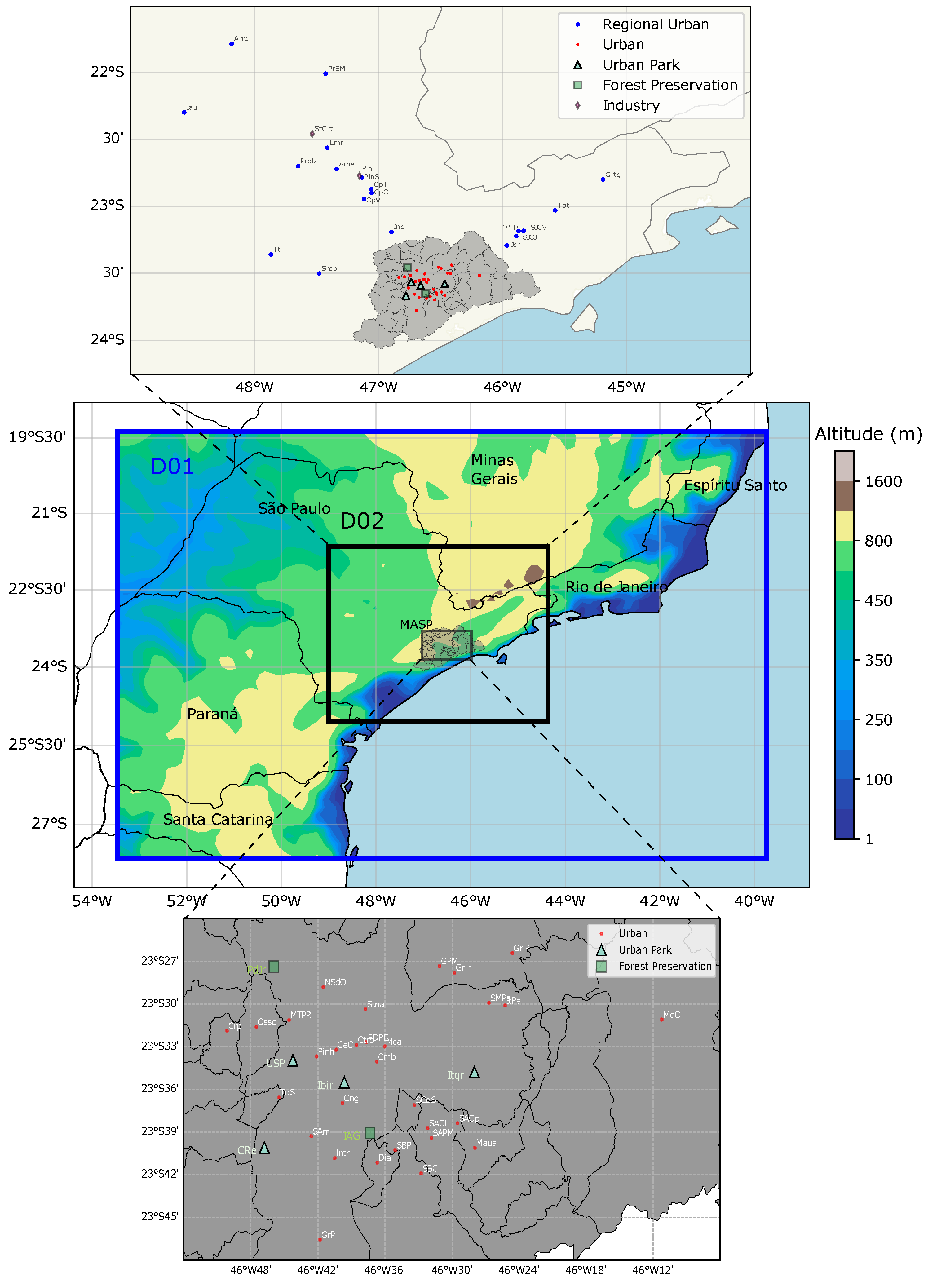
2.1. Case Study and Data Collection

The authors established two modeling domains with horizontal resolutions of 15 km and 3 km, respectively, as depicted in Figure 1. The meteorological files used as initial and boundary conditions (IC/BC) come from the NCEP FNL Operational Model Global Tropospheric Analyses (ds083.2, https://rda.ucar.edu/datasets/ds083.2/, accessed on 8 February 2020). Future scenario simulations used as meteorological IC/BC two global projections datasets from the NCAR’s Community Earth System Model (CESM1) Global Bias-Corrected CMIP5 Output to Support WRF/MPAS Research (ds316.1, https://rda.ucar.edu/datasets/ds316.1/, accessed on 31 January 2020), which is already in an intermediate file format for the WRF-Chem model. Both datasets present information every six hours with 1-degree by 1-degree horizontal resolution and 26 vertical levels from 1000 to 10 millibars [33,34]. To ensure the accuracy of the results, we conducted simulations for the first seven days of September 2018 and 2030, preceded by a two-day spin-up period on 30 and 31 August 2018 and 2030. The meteorological simulation was restarted 24 h before the next five days of analysis data, using the previous chemistry configuration to complete two months. This method is an adaptation proposed by Ritter [35] with some changes of additional 12 h before the 5-day steps.
The State of São Paulo Environmental Company (CETESB, for its acronym in Portuguese) is responsible for environmental quality control and analysis. CETESB also monitors the air quality conditions (surface O 3 , nitrogen oxide (NO), nitrogen dioxide (NO 2 ), sulfur dioxide (SO 2 ), particulate matter less than 10 micrometers (PM 10 ), PM 2.5 , benzene, and toluene in μ g m−3, and carbon monoxide (CO) in ppm). The air quality station network covers 61 locations, 37 in the MASP, as shown in Figure 1. The CETESB stations do not provide hourly accumulated rainfall data. Many do not meet WMO [36] guidelines for wind direction monitoring because the main objective of CETESB is to monitor air quality conditions. To compare with the model simulations for weather parameters, the authors used hourly data from the IAG/USP climatological station, which meets the WMO standards and has sensors free from urban and natural obstacles, including wind speed and direction. We classified the air quality stations by their surrounding areas, such as “Forest Preservation”, “Urban”, and “Urban Park” inside the MASP (coordinates are available in Supplementary Table S1), and outside the stations present two types as “Regional Urban” and “Industry” (Supplementary Table S2). This classification differs from CETESB, which considers only industrial or urban features.
The authors used two datasets of meteorological parameters and air pollutants as hourly time series from the CETESB repository (available online on the QUALAR website https://qualar.cetesb.sp.gov.br/qualar, accessed on 16 June 2020). The first dataset used hourly data from ten stations (Table S2 in Supplementary Materials) for five years (2014–2018). To choose the simulation period, we began by processing the five-year time series of hourly ozone concentrations and calculated the maximum hourly average monthly concentrations by station type. The second dataset comprises hourly concentrations taken at all stations within the second domain for two months (September and October 2018). We compared the hourly and maximum daily 8 h average (MDA8) O 3 concentrations by station types between scenarios (Base case, RCP 4.5, and RCP 8.5). Finally, the mean difference analysis of the MDA8 O 3 by month and space identifies future changes due to variations in the atmospheric conditions across the RCP scenarios. Table 1 displays the main physical and chemical configurations for two domains used for the three atmospheric scenario conditions.

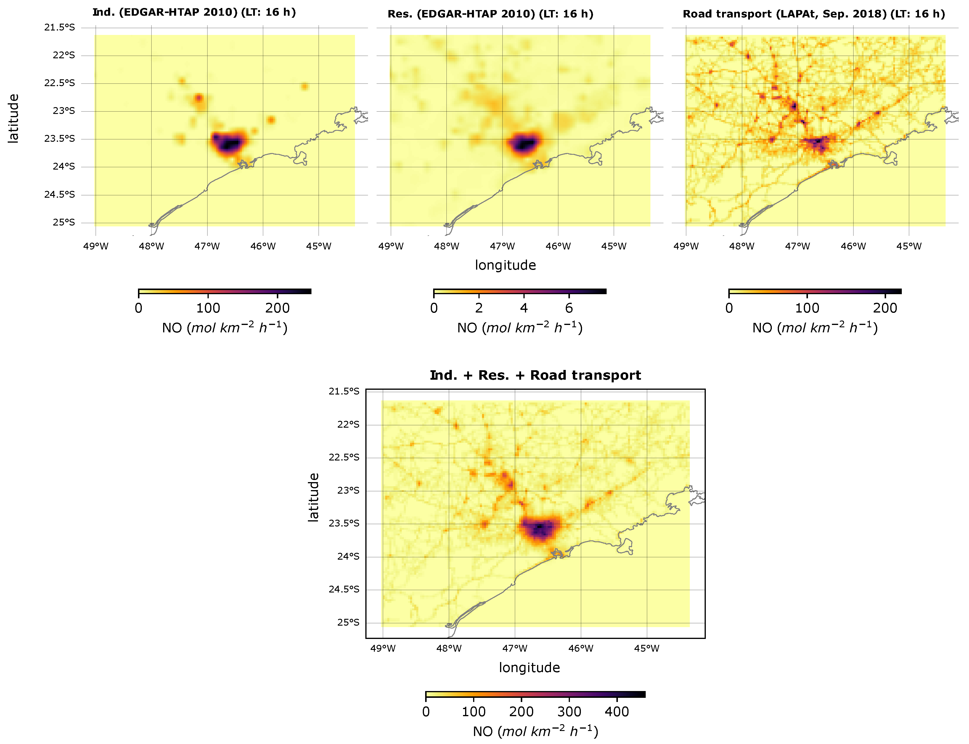
2.2. Preparation of the Emission Files

Emissions files included information from EDGAR v4.3 with HTAP v2.2 [51,52], local estimates for road transport emissions [22] and biogenic emissions from the Model of Emissions of Gases and Aerosols from Nature (MEGAN) [50]. All scenarios used the emission files under the CBMZ mechanism. The authors performed the model evaluation for the base case scenario using all measurements for the stations inside the second modeling domain area (D02 in Figure 1) and applying the statistical benchmarks by Emery et al. [53].
Test simulations to calibrate the emission file were performed for the base case scenario and comprised 6–12 and 24–28 September 2018, in conditions with no precipitation. The emission files for the road transport sector with a correction factor of 0.8 for NO x emissions improved the simulations for ozone and its precursors (i.e., NO x and CO). We used these corrected emission files to perform the two-month simulation period (August and September 2018) for all scenarios. The projected scenarios (RCP 4.5 and RCP 8.5) share the same information and configurations as the base case scenario.
From the many emission sources in the MASP, we count three as the most representative: road transport, industrial, and residential sectors. Road transport is responsible for the emission of most air pollutants [9]: 97% of CO, 75% of total hydrocarbon (HC), 64% of NO x , 17% of sulfur oxides (SO x ), and 40% of particulate matter (PM) for 2018 [11]. Heavy-duty vehicles (diesel-fueled) are responsible for 44% of NO x emissions. Our study used a bottom-up approximation described and applied in Andrade et al. [22] to calculate emissions by vehicle and fuel consumption types. This approximation involved data on road length (major roads, minor roads, and highway links) from OpenStreetMap contributors [54], vehicle numbers obtained from DENATRAN, and the CETESB [8] report’s vehicle fleet composition. We also used emission factors (Table S3 in Supplementary Materials) based on measurements in tunnel experiments (Jânio Quadros and Maria Maluf tunnels) presented in Pérez-Martínez et al. [55] and Andrade et al. [22], Andrade et al. [56].
The industrial sector also contributes to air pollutant emissions, with most point sources located in the MASP Southeast (i.e., the industrial park in Cubatão near the coast). The residential sector considers contributions from wood burning from restaurants and bakeries. These residential sources contribute locally and should be considered in emission inventories, as Lima et al. [10] mentioned. To represent these sources, we used emission inventories of these two sectors from the EDGAR-HTAP [51,52] for the 2010 reference year. We created a WRF-Chem emission file for a standard day by adding emissions from the road transport, industrial and residential sectors. The emission file speciation followed the CBMZ mechanism.
Figure 2 shows an example of the spatial emission distribution for NO. Industry (Ind.) and residential (Res.) emissions correspond to EDGAR-HTAP dataset for 2010, so hourly emissions are constant. Road transport considered the vehicle fleet for September–October 2018 and an hourly temporal profile from Andrade et al. [22]. Road transport emissions, depicted as line sources, predominate in the modeling domain area. The industrial and residential sources have the highest emission rates in urban areas at the center of the model domain area. Finally, the MEGAN model, version 2 [50], calculated biogenic emissions based on the ambient temperature, solar radiation, leaf area index, and plant functional type.

2.3. Model Performance Evaluation for the Base Case Scenario

The authors compared the meteorological and air quality model results against observations from CETESB air quality stations and the IAG/USP station. This comparison covers three recommended analyses suggested by Seinfeld and Pandis [57] for air pollutants: time series analysis, simulated peak concentrations, and comparisons by location. The meteorological evaluation considered benchmarks statistics (Supplementary Table S4) recommended by Monk et al. [58] for complex terrain due to characteristics of the modeling domain, such as higher areas that differ in elevation (e.g., mountains as Pico do Jaraguá and buildings in the MASP).
On the other hand, there are many performance statistics parameters to evaluate simulations from air quality models. Emery et al. [53] analyzed statistics and benchmarks to assess photochemical models applied to North America, shown in Supplementary Table S4. For surface ozone, they recommended two benchmarks as “Goal” and “Criteria” levels and three performance statistics: normalized mean bias (NMB), normalized mean error (NME), and correlation coefficient (r). Table S5 in the Supplementary Materials shows these and other statistical equations used in the meteorological performance evaluation: mean absolute gross error (MAGE), mean bias (MB), index of agreement (IOA), and root-mean-square error (RMSE). They also recommend only a cutoff value for hourly ozone to calculate NMB and NME statistics to avoid skewing issues. In contrast, the correlation coefficient calculation requires all the hourly simulations. Therefore, we used a cutoff value of 40 ppb (80 μ g m−3) to calculate NMB and NME statistics for the surface ozone; this threshold represents higher levels achieved in spring in the MASP.

3. Results and Discussions

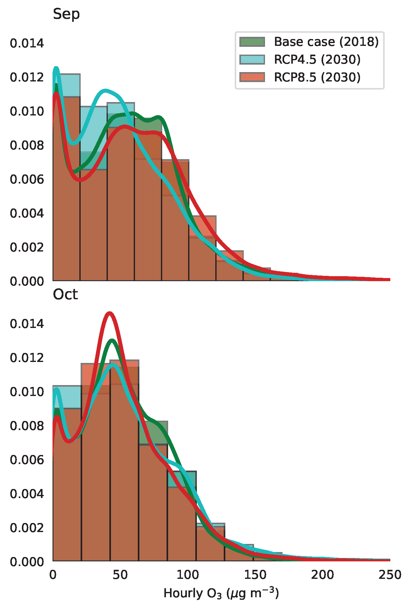
3.1. Monthly Ozone Analysis

The authors selected air quality stations with available hourly information from CETESB stations, as shown in Table S6 in the Supplementary Materials. This analysis reveals higher ozone levels, mainly in September to December, as shown in Figure 3. The highest average value for spring agrees with Carvalho et al. [13], who mentioned that the increase in O 3 formation appears mainly between September and November due to the clear sky conditions during the afternoon. The daily profile analysis shows higher ozone peaks at 15:00 h Brazil local time (LT), mainly during September for several air quality station types. Therefore, September and October are months regarded as modeling periods to study ozone formation.
Furthermore, clear sky conditions can reduce the ozone flux through stomatal conductance by the forest ecosystem [59], which is another factor to consider. In contrast, the opposite occurs during the summer under cloudy or partly cloudy conditions. However, there are no notable differences in O 3 concentrations between stations surrounded by vegetation, such as those located in forest preservation and urban park. For instance, Pico do Jaraguá (Forest preservation station), which is surrounded by forest that could potentially remove O 3 concentrations [60], showed no significant difference in O 3 (Figure 3) when compared to other stations with less vegetation, such as those classified as urban (i.e., Interlagos, Carapicuíba, Parque D.Pedro II, Pinheiros).

3.2. Base Case Scenario

3.2.1. Meteorological Model Performance Evaluation

The authors compared the meteorological parameters of the base case scenario simulation with measurements at the IAG/USP climatological station (Água Funda). Supplementary Figure S1 shows comparisons at the surface of temperature ( C), relative humidity (%), accumulated rain (mm), and winds (speed in m s 1 and direction in degrees). Statistical results in Supplementary Table S7 show at least inaccuracies in the MB temperature benchmark ( ± 1 C) and wind speed for two benchmarks (IOA > 6 and MB ± 1.5 m s 1 ). On average, model simulations for these parameters overestimated the observations, in which MB values were 1.56 C and 1.69 m s 1 , respectively. Statistical results for relative humidity and wind direction comply in good agreement with all benchmarks for complex terrain.
The accumulated rainfall in September was 107 mm, lower than in October (152.2 mm). Supplementary Figure S2 shows differences between simulations and observations with higher daily overestimations (38 days) than underestimations (20 days). Some underestimations were also noticed, primarily due to the model’s inability to reproduce rain peaks. Overall, the hourly rain simulations overestimated the observations, with a mean bias of 0.13 mm. The correlation coefficient between the simulated and observed rainfall was low (r = 0.11). However, it indicated a statistically significant linear relationship between the two sets of values (t-stat = 4.23 > t-crit = 1.96), as confirmed by the Pearson correlation’s t-test with the significance level of alpha = 0.05 and n-2 degrees of freedom.
Wind-rose plot comparisons between simulation and observations presented similar directions (Figure S3 in Supplementary Materials), mainly for winds blowing from southeasterly influenced by sea breezes. However, simulations did not represent the frequency of easterly winds. Moreover, the frequency of calm wind for observations (values < 0.5 m s 1 ) was higher than the modeled values. The wind speed simulations frequently exceeded the observations, with a higher value in October, reaching a maximum difference of 6.48 m s 1 , as shown in Figure S2. The model consistently overestimated the wind speed by 1.69 m s 1 on average.

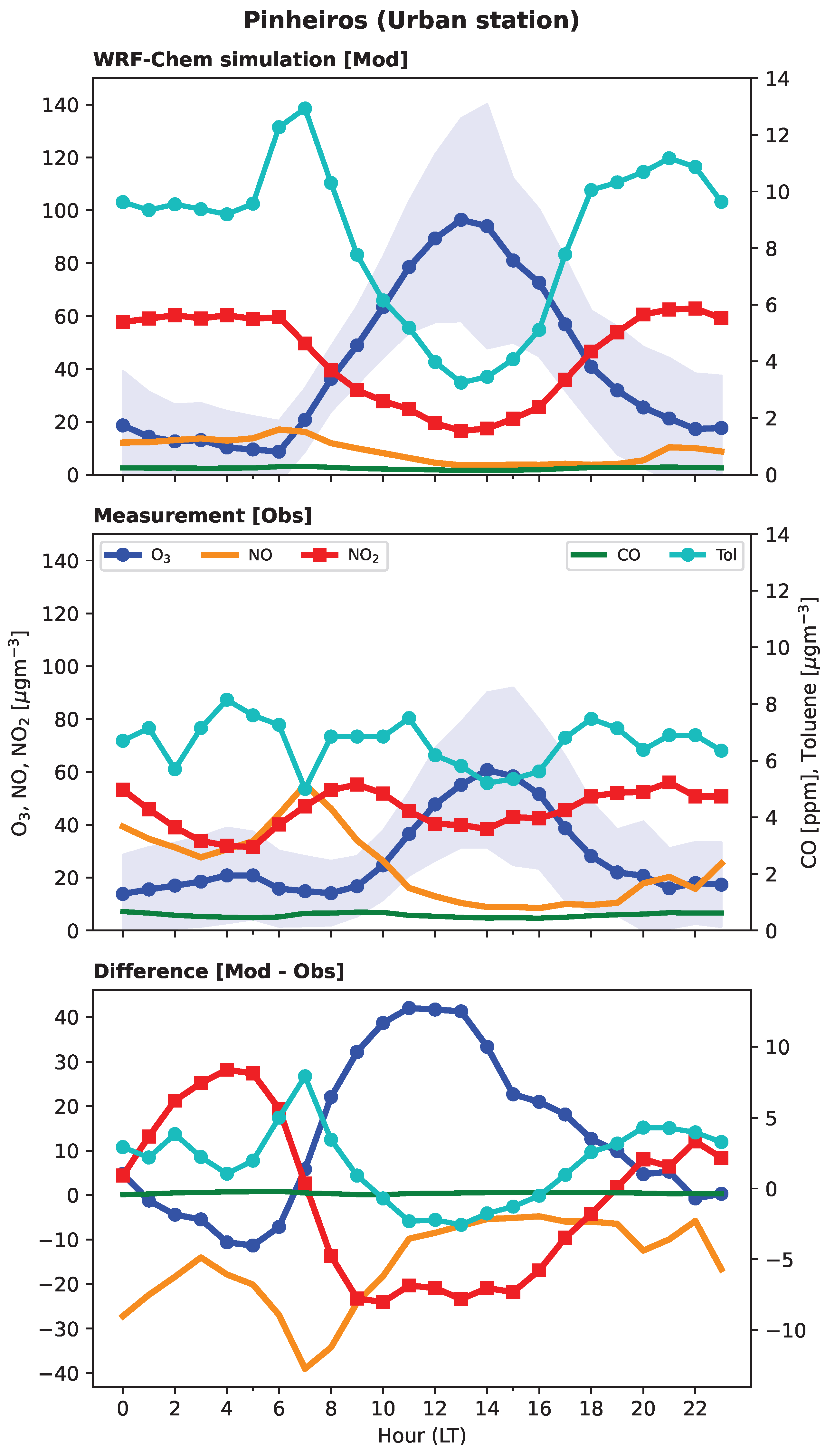
3.2.2. Air Quality Model Performance Evaluation

The authors compared simulations against observations as a mean daily profile for O 3 , NO, NO 2 , CO, and toluene (Figure 4) for the Pinheiros station, as it has complete measurements for all air quality parameters. Some pollutants (NO x and toluene) with remarkable differences for certain hours at Pinheiros station overestimated the observations caused by the temporal–spatial distribution of the emissions and uncertainties of temperature and wind speed simulations. Toluene simulations are overestimated during nighttime and underestimated during daylight, indicating that VOC emissions may be overestimated, which can impact ozone formation during noon hours. In addition, NO 2 uncertainties can affect the nocturnal peak ozone simulation around three- and seven-hours LT, a behavior reported by Andrade et al. [9], Carvalho et al. [13], and Mazzoli da Rocha [27].
Supplementary Table S8 shows values of the performance statistics considering all stations inside the 3 km domain. Overall, simulations for O 3 and NO 2 overestimated the observations with MB values within 13.15 μ g m−3 (October 2018) and 4.09 μ g m−3 (September 2018), respectively. NO and CO simulations underestimated the measurements for October 2018, with NMB within −47.84% and −61.76%, respectively. Some factors can explain these differences for those pollutants, attributed to the spatial emission distribution for light-duty and heavy-duty vehicles around specific roads in the MASP, as mentioned by Ibarra-Espinosa et al. [61]. Heavy-duty diesel vehicles travel long distances and release more NO x than other vehicle types. This behavior was not represented in the emission approximation used in this study and reported in Andrade et al. [22], which assumes a proportional distribution based on the total road length (i.e., motorway, trunk, primary, secondary, and tertiary road types) for each grid cell of the modeling domain. The hourly ground ozone concentrations simulation did not attain a correlation coefficient greater than 0.7. However, ozone simulations comply with the statistical benchmarks suggested by Emery et al. [53], whose values are marked in blue in Supplementary Table S8. The overestimation of NMB with a cutoff value for O 3 is slightly greater in September than in October, suggesting that the simulation of peak ozone concentrations in October is more accurate.

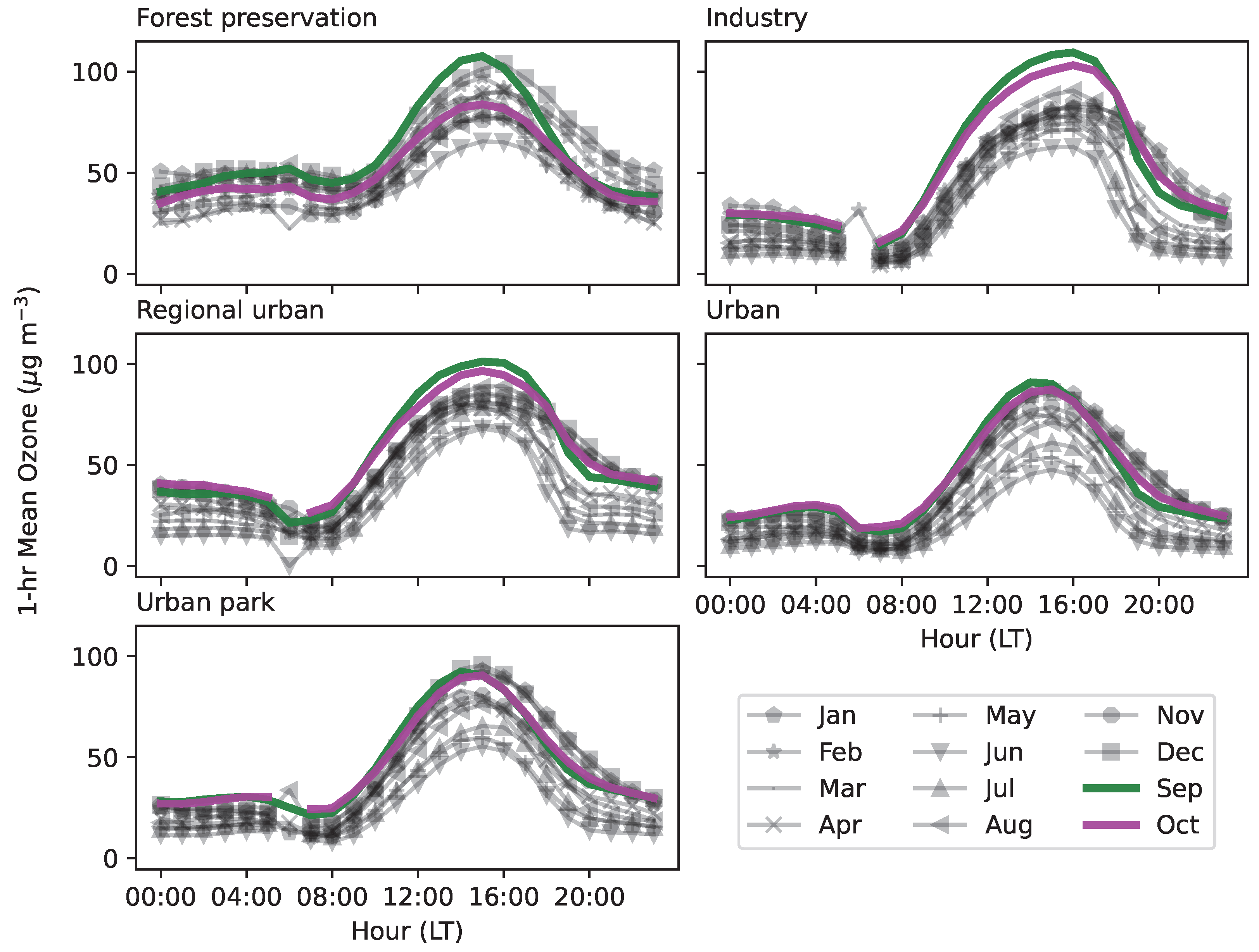
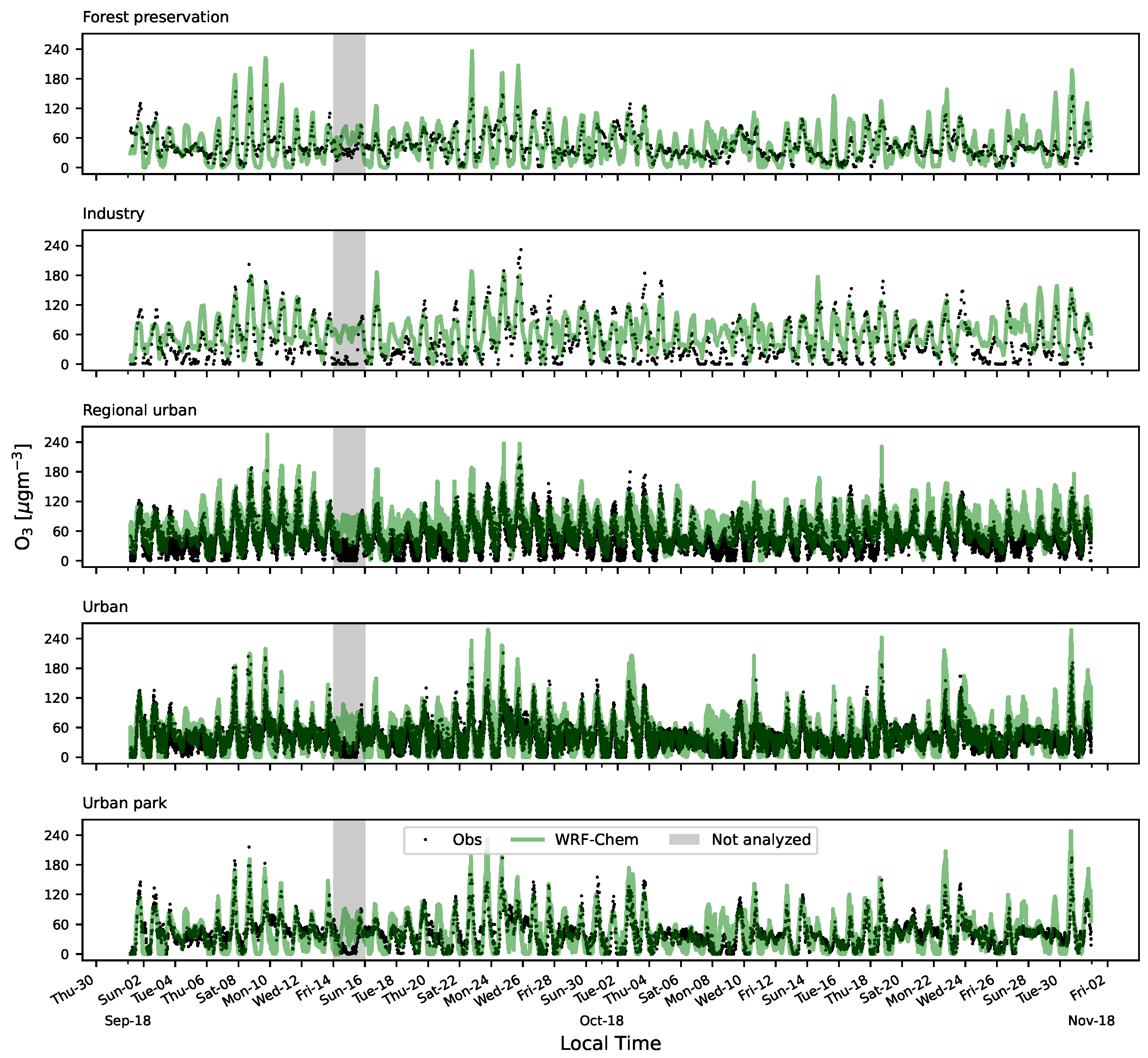
3.2.3. Surface Ozone Evaluation by Station Type

The authors compared the hourly O 3 simulations against the observations by the station for September and October 2018 (Figure 5). Hourly simulations reached higher observations in each plot. This consideration is essential for model validation, according to suggestions by Seinfeld and Pandis [57]. Table 2 presents a summary of the statistical results by station type and month that evaluates the performance of the surface ozone simulation, including all stations inside the second model domain. Applying the evaluation proposed by Emery et al. [53], O 3 simulations for many stations complied with at least two statistical benchmarks for the criteria level. These statistical results for both months suggest a good agreement with the observations. The forest preservation (FP) station had a noticeable NME value in red that exceeded the statistical benchmark. However, this station type presented low MB (0.45 μ g m−3) and high correlation coefficient (r = 0.72), shown in Supplementary Table S9. Based on statistical values for higher r and IOA and low MB (close to 0), O 3 simulations for September 2018 presented a better performance than October. A reasonable explanation for the low correlation for October 2018 simulations is the model limitations to represent rainy and cloudy conditions that impact the O 3 formation.
Peak ozone concentrations for industry stations outside the MASP are underestimated, achieving the criteria benchmark (NMB <±15%) for both months. However, ozone simulations for regional urban stations were more accurate, with NMB values within the goal benchmark (<±5%). Inside the MASP, urban park stations showed good simulations for both months, while the FP station performed better in October than in September. Peak ozone simulations for urban stations presented acceptable overestimations, with NMB values within the goal benchmark (<±15%). These statistical results indicate a good performance of the model in simulating higher hourly observation values, in line with Seinfeld and Pandis [57] suggestion to represent peak concentrations.

3.3. Future Scenarios

3.3.1. Changes in Meteorological Conditions

Monthly temperature and relative humidity simulations for September and October (Figures S4 and S5 in Supplementary Materials) show different values by scenarios and air quality stations. The RCP 8.5 scenario has a prevailing higher monthly mean temperature. In September 2030, the increase in temperature under the RCP 8.5 scenario is more pronounced, compared to October 2030. The temperature values for the base case are nearly identical to the RCP 4.5 scenario, particularly in September, suggesting that the RCP 4.5 scenario may be optimistic for the São Paulo state and the future may be worse as projected by the RCP 8.5 scenario. Hence, these changes in temperature impact the model because they influence biogenic emissions, positively increasing O3 formation in the MASP. Thus, the MEGAN model estimates the increase in isoprene emissions for September as a response to changes in rising temperature and other factors mentioned previously.
As part of the base case scenario, the authors found the highest value at the Pico do Jaraguá station, with a relative humidity of 85.3% for October 2018. Low values for the RCP 8.5 scenario are remarkable in both months, below 70% on average for all stations. As in the case of temperature, the relative humidity for September presented similar values for the base case and RCP 4.5 scenarios. Regarding accumulated rain (Figure S6 in Supplementary Materials), September showed similar rainy patterns between scenarios. However, rainy days in October were not comparable between scenarios. Model simulations for the RCP 4.5 scenario depict the highest accumulated daily rainfall peak from 20 to 24 September 2030. Rainfall patterns varied significantly in October, with only a few coincidences between the two scenarios: one on 13 October (Base case and RCP 8.5) and the other on 17 October (base case and RCP 4.5). The monthly rainfall in October is greater than in September, as demonstrated in Supplementary Figure S6. Additionally, the simulation results for RCP 4.5 and RCP 8.5 scenarios indicate a reduction in monthly rainfall. The RCP 8.5 scenario exhibited a more pronounced decrease than the base case and RCP 4.5 scenarios.

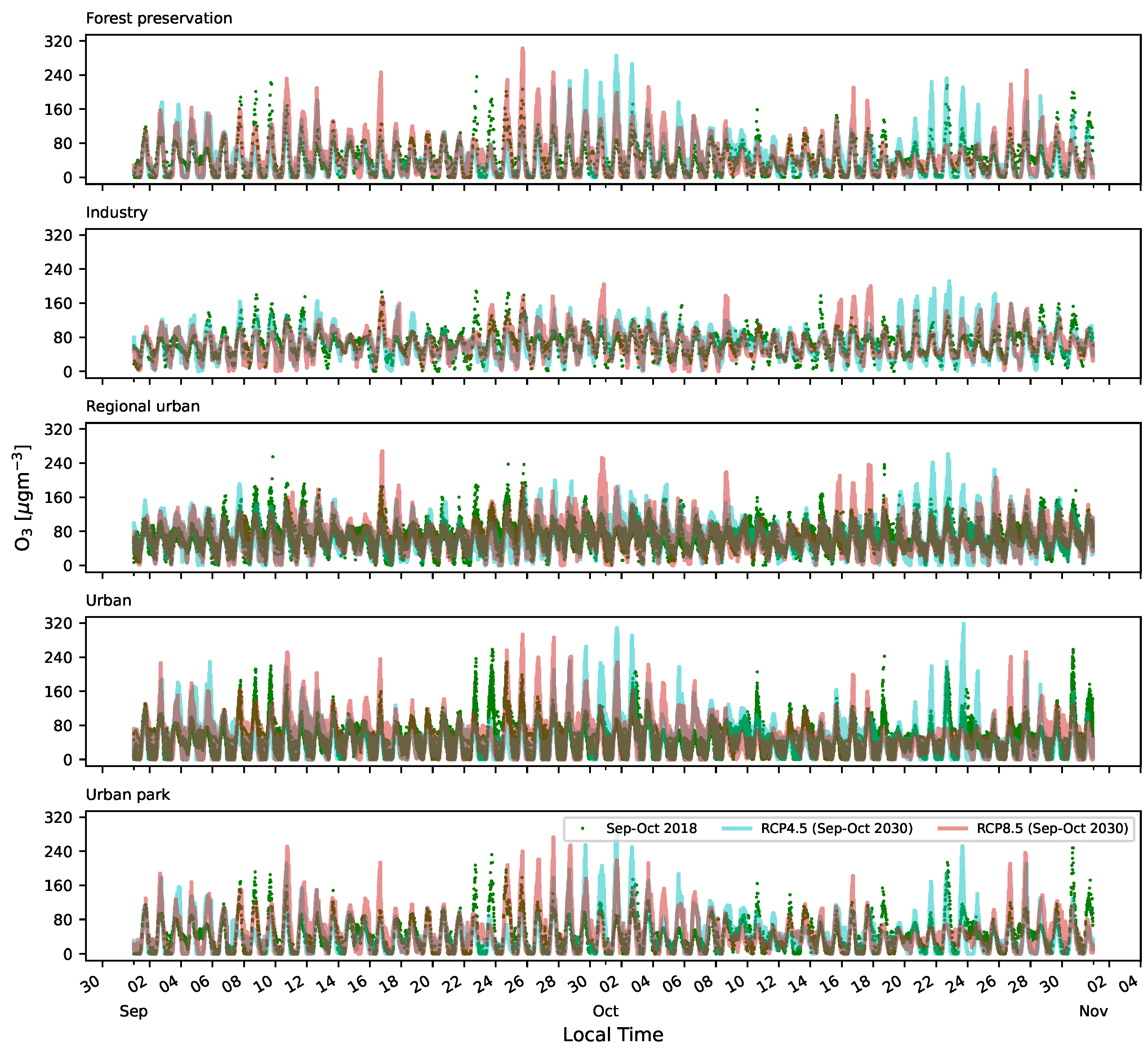
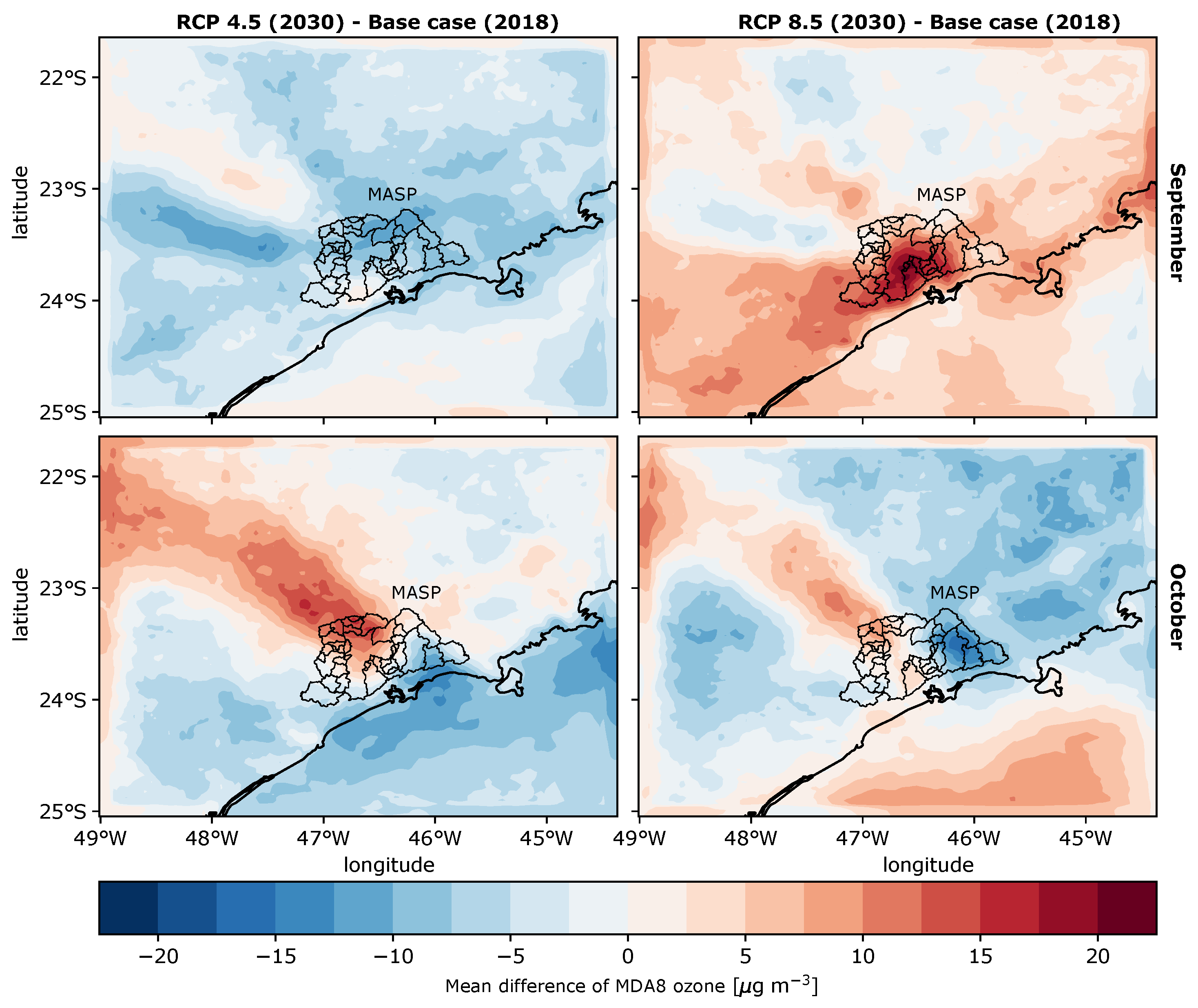
3.3.2. Changes in Surface Ozone

Figure 6 compares the time series of simulated surface O 3 concentrations between the base case (September–October 2018) and the RCP 4.5 and 8.5 scenarios for September–October 2030. RCP 4.5 and 8.5 scenarios have different atmospheric conditions with the same anthropogenic emissions calculated for September–October 2018. Only a few days under the base case scenario have three periods with high O 3 concentrations: 8–11, 22–24 September and 30–31 October. In contrast, the authors found hourly peak concentrations for both RCP scenarios. For September’s last days, the RCP 4.5 scenario simulations showed the O 3 peak predominantly in stations inside the MASP (Forest preservation, Urban, and Urban park). Trends of O 3 peak increment for October are pronounced in all station types during its first days and between 20 to 26 October 2030. The highest peak simulation for urban stations achieved 318.4 μ g m−3 at 15 h LT in the Guarulhos-Paço Municipal station on 23 October 2030. Hence, low rain simulations under the RCP 4.5 (Supplementary Figure S6) between 19 and 29 October 2030 influenced a higher ozone formation than the RCP 8.5.
Conversely, rising ground O 3 under the RCP 8.5 scenario is higher for September than October, mainly in the MASP stations. Figure 7 illustrates a higher frequency for values greater than 100 μ g m−3 of hourly ozone concentrations in September compared to October under the RCP 8.5 scenario. There is a noticeable peak density for values around 50 μ g m−3 under the RCP 8.5 scenario in October. Overall, the simulations for September showed a decrease in ozone formation for the RCP 4.5 scenario, particularly in the MASP, whereas the simulations for the RCP 8.5 scenario showed an increase. The trend for the RCP 4.5 scenario was previously confirmed by Schuch et al. [28] for 2030 simulations, considering both mitigation strategies for anthropogenic emission (mitigation scenario and maximum feasible reduction).
The analysis confirmed the increase in MDA8 O 3 for both RCP 4.5 and RCP 8.5 scenarios under low rainfall conditions. Figure 8 reveals that the monthly average for September is higher in the RCP 8.5 scenario than the RCP 4.5, which shows prominent decreases. The selected areas in the north of the second modeling domain for the RCP 8.5 scenario in September showed minor reductions, while the urban center could experience significant increases, shown in Table 3 for urban station types. Whereas for October, the authors found increases and decreases for both RCP scenarios. For the RCP 4.5 scenario, we observed the influence of the sea breeze, which transports O 3 from the center of MASP to northwest locations. MDA8 O 3 reductions are also notable in some urban areas for both RCP scenarios, particularly in the northeast of the MASP during September and in the east zone (i.e., Mogi das Cruzes, Biritiba Mirim, and Salesópolis) as well as the southwest (Juquitiba) during both months. October presented more cloudy days, and a few temperature increments influenced each scenario differently, both associated with varying rain patterns between scenarios. The RCP 8.5 scenario did not increase the ozone concentration for October more than the RCP 4.5. So, cloudy conditions are one of the main drivers that impact the photochemical reactions in air quality simulations. Table 4 compares changes in the percentage of ozone concentration for the MASP. The simulations conducted for September in this study are consistent with those of previous studies, despite the different periods considered. Mazzoli da Rocha [27] reported a similar decrease in ozone concentration for the optimistic scenario, as observed in this study for September, while a higher increase percentage was reported for the pessimistic scenario. However, this difference is reasonable, as the comparison was made with the year 2050 instead of 2030. Notably, our simulations for October reveal a more significant increase in ozone concentration for the optimistic scenario, whereas previous studies reported decreased concentrations for days in July–August [28] and November [27].

4. Conclusions

The WRF-Chem model is an effective tool for analyzing ozone formation and its changes in meteorological conditions. It can explain the factors contributing to air pollutant formation in urban areas and how pollutants may vary under different weather conditions while keeping anthropogenic emission constant. Our methodology approximates the total emissions by adding other sources to the transport emissions, such as industry and residential from EDGAR-HTAP and biogenic sources from MEGAN for September and October 2018 (Base case). The WRF-Chem model simulated the O 3 formation and other air pollutants (NO x , CO, toluene) under two RCP (4.5 and 8.5) scenarios for September and October 2030. Compared with the base case scenario, the authors assessed their changes in atmospheric conditions and their impact on the ground O 3 formation. Our study provides the framework to analyze the interactions between climate change scenarios and air pollutants using a regional air quality model.
First, we evaluated the base case scenario, which showed O 3 simulations in good agreement with observations considering the benchmarks recommended by Emery et al. [53]. However, meteorological simulations for some parameters (temperature, wind speed, and rainy conditions) presented inaccuracies in compliance with performance statistics suggested by Monk et al. [58]. These limitations impacted the surface O 3 simulation. Other factors contributed to inaccuracies and are related to ozone’s precursors (NO x , CO, and VOC), mainly associated with the input emissions and their temporal and spatial distribution. Second, based on the comparisons between the RCP scenarios and the base case scenario, we found an average increase in peak ozone concentrations (0.43% for RCP 4.5 and 5.92% for RCP 8.5) with variations depending on the month and location. In September, O 3 simulations showed increases under the RCP 8.5 scenario atmospheric conditions of high-rising temperatures and low rainy conditions. RCP 4.5 scenario simulations showed that O3 decreased in September. However, their peak ozone concentrations in October presented more increases than under the RCP 8.5.
In conclusion, this study found monthly changes in surface O 3 over the MASP under the RCP 4.5 and RCP 8.5 scenarios as future atmospheric conditions, maintaining the emission rates and land use unchanged in 2030. Rising temperatures by radiative forcing scenarios do not necessarily lead to increases in ozone due to changes in rainfall patterns. Considering two months of analysis, on average, the RCP 8.5 showed higher O 3 concentrations than the RCP 4.5. However, based on a monthly analysis, the RCP 8.5 had lower O 3 concentrations in October than the RCP 4.5. Our work has limitations in simulating an extended period because of limited computational resources. Despite this, we recommend evaluating monthly changes in O 3 to obtain insights into the impacts of changes in atmospheric conditions. As a crucial reminder, society must be prepared for possible negative consequences under any climate change scenario. In this case, ozone formation can intensify or decrease depending on how meteorological factors, such as cloudiness and temperatures, vary.

Supplementary Materials

The following supporting information can be downloaded at: https://www.mdpi.com/article/10.3390/atmos14040626/s1, Table S1: Geographical coordinates and classification of the CETESB air quality monitoring stations and the IAG climatological station inside the Metropolitan Area of São Paulo (MASP); Table S2: CETESB air quality monitoring stations network around the Metropolitan Area of São Paulo, and inside the State of São Paulo; Table S3: Emission factors by vehicle type and fuel (g/km); Table S4: Surface ozone and meteorological parameters with statistic benchmarks; Table S5: Statistic equations used for the model evaluation; Table S6: CETESB stations with five years (2014–2018) of hourly measurements for monthly analysis; Table S7: Statistical analysis of meteorology parameters for September–October 2018 at IAG/USP station location; Table S8: Statistical performance analysis of air quality gas simulations by month; Table S9: Statistical performance analysis of surface ozone simulations by type of station and month; Figure S1: Comparison of observed and modeled meteorological parameters at IAG/USP Station for September–October 2018 (Reprinted/adapted with permission from Ref. [37]. 2021, Universidade de São Paulo); Figure S2: Differences between simulation (Mod) and observations (Obs) for daily total rain, based on measurements at the IAG/USP climatological station during Sep-Oct 2018; Figure S3: Wind rose plot comparison between modeled (Mod.) vs. observations (Obs.) at the IAG/USP climatological station for the period September–October 2018; Figure S4: Comparison of average monthly temperature values among scenarios by station locations. (a) September, (b) October (Reprinted/adapted with permission from Ref. [37]. 2021, Universidade de São Paulo); Figure S5: Comparison of average monthly relative humidity values among scenarios by station locations. (a) September, (b) October (Reprinted/adapted with permission from Ref. [37]. 2021, Universidade de São Paulo); Figure S6: Accumulated daily (up) and monthly (down) rainfall comparison between scenarios at the IAG/USP climatological station (Reprinted/adapted with permission from Ref. [37]. 2021, Universidade de São Paulo).

Author Contributions

Conceptualization, M.d.F.A. and M.G.-C.; methodology, A.H.D.P. and M.G.-C.; software, A.H.D.P.; validation, A.H.D.P., M.G.-C. and M.d.F.A.; formal analysis, A.H.D.P.; investigation, A.H.D.P.; writing—original draft preparation, A.H.D.P.; writing—review and editing, A.H.D.P., M.G.-C. and M.d.F.A.; visualization, A.H.D.P.; supervision, M.d.F.A.; project administration, A.H.D.P.; funding acquisition, CAPES and IAG/USP. All authors have read and agreed to the published version of the manuscript.

Funding

This research was funded by Coordenação de Aperfeiçoamento de Pessoal de Nível Superior (CAPES) for the master study fellowship at IAG-USP.

Institutional Review Board Statement

Not applicable.

Informed Consent Statement

Not applicable.

Data Availability Statement

We used Python scripts to extract outputs simulations from the WRF-Chem model and download measured data from QUALAR website. The scripts and data (raw and processed) are available at https://github.com/adelgadop/Master_dissertation, updated on 1 December 2021.

Acknowledgments

The authors acknowledge the computer resources provided by the IAG Institute to run the WRF-Chem model and for the meteorology information from the IAG station. We recognize the São Paulo Environmental Agency (CETESB) for providing information through its QUALAR webpage. Finally, we acknowledge the support from the CAPES funding for the master study fellowship at IAG-USP.

Conflicts of Interest

The authors declare no conflict of interest.

References

  1. WHO. WHO Global Air Quality Guidelines. Particulate Matter (PM2.5 and PM10, Ozone, Nitrogen Dioxide, Sulfur Dioxide and Carbon Monoxide; Licence: CC BY-NC-SA 3.0 IGO; World Health Organization: Geneva, Italy, 2021. [Google Scholar]
  2. Nuvolone, D.; Petri, D.; Voller, F. The effects of ozone on human health. Environ. Sci. Pollut. Res. 2018, 25, 8074–8088. [Google Scholar] [CrossRef] [PubMed]
  3. Sampedro, J.; Waldhoff, S.T.; Van de Ven, D.J.; Pardo, G.; Van Dingenen, R.; Arto, I.; del Prado, A.; Sanz, M.J. Future impacts of ozone driven damages on agricultural systems. Atmos. Environ. 2020, 231, 117538. [Google Scholar] [CrossRef]
  4. IPCC. Climate Change 2013: The Physical Science Basis. Contribution of Working Group I to the Fifth Assessment Report of the Intergovernmental Panel on Climate Change; Cambridge University Press: Cambridge, UK; New York, NY, USA, 2013; p. 1535. [Google Scholar]
  5. Fiore, A.M.; Naik, V.; Leibensperger, E.M. Air Quality and Climate Connections. J. Air Waste Manag. Assoc. 2015, 65, 645–685. [Google Scholar] [CrossRef]
  6. Fu, T.M.; Tian, H. Climate Change Penalty to Ozone Air Quality: Review of Current Understandings and Knowledge Gaps. Curr. Pollut. Rep. 2019, 5, 159–171. [Google Scholar] [CrossRef] [Green Version]
  7. IBGE. População das Regiões Metropolitanas no 2019. 2019. Available online: https://agenciadenoticias.ibge.gov.br/agencia-detalhe-de-midia.html?view=mediaibge&catid=2103&id=3109 (accessed on 20 October 2021).
  8. CETESB. Emissões Veiculares no Estado de São Paulo 2018; Série Relatórios: São Paulo, Brazil, 2019; p. 193. [Google Scholar]
  9. Andrade, M.d.F.; Kumar, P.; de Freitas, E.D.; Ynoue, R.Y.; Martins, J.; Martins, L.D.; Nogueira, T.; Perez-Martinez, P.; de Miranda, R.M.; Albuquerque, T.; et al. Air quality in the megacity of São Paulo: Evolution over the last 30 years and future perspectives. Atmos. Environ. 2017, 159, 66–82. [Google Scholar] [CrossRef] [Green Version]
  10. Lima, F.D.M.; Pérez-Martínez, P.J.; de Fatima Andrade, M.; Kumar, P.; de Miranda, R.M. Characterization of particles emitted by pizzerias burning wood and briquettes: A case study at Sao Paulo, Brazil. Environ. Sci. Pollut. Res. 2020, 27, 35875–35888. [Google Scholar] [CrossRef]
  11. CETESB. Qualidade do ar no Estado de São Paulo 2018, 21st ed.; Série Relatórios: São Paulo, Brazil, 2019; p. 214. [Google Scholar]
  12. Chiquetto, J.B.; Silva, M.E.S.; Cabral-Miranda, W.; Ribeiro, F.N.D.; Ibarra-Espinosa, S.A.; Ynoue, R.Y. Air Quality Standards and Extreme Ozone Events in the São Paulo Megacity. Sustainability 2019, 11, 3725. [Google Scholar] [CrossRef] [Green Version]
  13. Carvalho, V.S.B.; Freitas, E.D.; Martins, L.D.; Martins, J.A.; Mazzoli, C.R.; Andrade, M.d.F. Air quality status and trends over the Metropolitan Area of São Paulo, Brazil as a result of emission control policies. Environ. Sci. Policy 2015, 47, 68–79. [Google Scholar] [CrossRef]
  14. Von Schneidemesser, E.; Monks, P.S.; Allan, J.D.; Bruhwiler, L.; Forster, P.; Fowler, D.; Lauer, A.; Morgan, W.T.; Paasonen, P.; Righi, M.; et al. Chemistry and the Linkages between Air Quality and Climate Change. Chem. Rev. 2015, 115, 3856–3897. [Google Scholar] [CrossRef]
  15. De Lima, G.N.; Magaña Rueda, V.O. The urban growth of the metropolitan area of Sao Paulo and its impact on the climate. Weather Clim. Extrem. 2018, 21, 17–26. [Google Scholar] [CrossRef]
  16. Marengo, J.; Valverde, M.; Obregon, G. Observed and projected changes in rainfall extremes in the Metropolitan Area of São Paulo. Clim. Res. 2013, 57, 61–72. [Google Scholar] [CrossRef] [Green Version]
  17. Marengo, J.A.; Ambrizzi, T.; Alves, L.M.; Barreto, N.J.C.; Reboita, M.S.; Ramos, A.M. Changing Trends in Rainfall Extremes in the Metropolitan Area of São Paulo: Causes and Impacts. Front. Clim. 2020, 2, 8–20. [Google Scholar] [CrossRef]
  18. Nobre, C.A.; Marengo, J.A.; Soares, W.R. (Eds.) Climate Change Risks in Brazil; Springer International Publishing: Cham, Switzerland, 2019; p. 219. [Google Scholar] [CrossRef]
  19. Van Vuuren, D.P.; Edmonds, J.; Kainuma, M.; Riahi, K.; Thomson, A.; Hibbard, K.; Hurtt, G.C.; Kram, T.; Krey, V.; Lamarque, J.F.; et al. The representative concentration pathways: An overview. Clim. Change 2011, 109, 5–31. [Google Scholar] [CrossRef]
  20. Thomson, A.M.; Calvin, K.V.; Smith, S.J.; Kyle, G.P.; Volke, A.; Patel, P.; Delgado-Arias, S.; Bond-Lamberty, B.; Wise, M.A.; Clarke, L.E.; et al. RCP4.5: A pathway for stabilization of radiative forcing by 2100. Clim. Change 2011, 109, 77–94. [Google Scholar] [CrossRef] [Green Version]
  21. Riahi, K.; Rao, S.; Krey, V.; Cho, C.; Chirkov, V.; Fischer, G.; Kindermann, G.; Nakicenovic, N.; Rafaj, P. RCP 8.5—A scenario of comparatively high greenhouse gas emissions. Clim. Change 2011, 109, 33–57. [Google Scholar] [CrossRef] [Green Version]
  22. Andrade, M.D.F.; Ynoue, R.Y.; Freitas, E.D.; Todesco, E.; Vara Vela, A.; Ibarra, S.; Martins, L.D.; Martins, J.A.; Carvalho, V.S.B. Air quality forecasting system for Southeastern Brazil. Front. Environ. Sci. 2015, 3, 6975. [Google Scholar] [CrossRef] [Green Version]
  23. Sánchez-Ccoyllo, O.R.; Ynoue, R.Y.; Martins, L.D.; Andrade, M.d.F. Impacts of ozone precursor limitation and meteorological variables on ozone concentration in São Paulo, Brazil. Atmos. Environ. 2006, 40, 552–562. [Google Scholar] [CrossRef]
  24. Hoshyaripour, G.; Brasseur, G.; Andrade, M.; Gavidia-Calderón, M.; Bouarar, I.; Ynoue, R. Prediction of ground-level ozone concentration in São Paulo, Brazil: Deterministic versus statistic models. Atmos. Environ. 2016, 145, 365–375. [Google Scholar] [CrossRef]
  25. Vara-Vela, A.; Andrade, M.F.; Kumar, P.; Ynoue, R.Y.; Muñoz, A.G. Impact of vehicular emissions on the formation of fine particles in the Sao Paulo Metropolitan Area: A numerical study with the WRF-Chem model. Atmos. Chem. Phys. 2016, 16, 777–797. [Google Scholar] [CrossRef] [Green Version]
  26. Vara-Vela, A.; de Fátima Andrade, M.; Zhang, Y.; Kumar, P.; Ynoue, R.Y.; Souto-Oliveira, C.E.; da Silva Lopes, F.J.; Landulfo, E. Modeling of Atmospheric Aerosol Properties in the São Paulo Metropolitan Area: Impact of Biomass Burning. J. Geophys. Res. Atmos. 2018, 123, 9935–9956. [Google Scholar] [CrossRef]
  27. Mazzoli da Rocha, C.R. Estudo Numérico da influência das Mudançãs Climáticas e das Emissões Urbanas no Ozônio Troposférico da Região Metropolitana de São Paulo. In Tese de Doutorado; Universidade de São Paulo: São Paulo, Brazil, 2013. [Google Scholar]
  28. Schuch, D.; Andrade, M.d.F.; Zhang, Y.; Dias de Freitas, E.; Bell, M.L. Short-Term Responses of Air Quality to Changes in Emissions under the Representative Concentration Pathway 4.5 Scenario over Brazil. Atmosphere 2020, 11, 799. [Google Scholar] [CrossRef]
  29. IPCC. Summary for Policymakers. In Climate Change 2021: The Physical Science Basis. Contribution of Working Group I to the Sixth Assessment Report of the Intergovernmental Panel on Climate Change; Summary for Policymakers: Cambridge, UK; New York, NY, USA, 2021; p. 39. [Google Scholar]
  30. Grell, G.A.; Peckham, S.E.; Schmitz, R.; McKeen, S.A.; Frost, G.; Skamarock, W.C.; Eder, B. Fully coupled ’online’ chemistry within the WRF model. Atmos. Environ. 2005, 39, 6957–6975. [Google Scholar] [CrossRef]
  31. Skamarock, W.C.; Klemp, J.B.; Dudhia, J.; Gill, D.O.; Liu, Z.; Berner, J.; Wang, W.; Powers, J.G.; Duda, M.G.; Barker, D.; et al. A Description of the Advanced Research WRF Model Version 4.1 (No. NCAR/TN-556+STR); National Center for Atmospheric Research: Boulder, CO, USA, 2019. [Google Scholar]
  32. Gavidia-Calderón, M.; Vara-Vela, A.; Crespo, N.; Andrade, M. Impact of time-dependent chemical boundary conditions on tropospheric ozone simulation with WRF-Chem: An experiment over the Metropolitan Area of São Paulo. Atmos. Environ. 2018, 195, 112–124. [Google Scholar] [CrossRef]
  33. Monaghan, A.J.; Steinhoff, D.F.; Bruyere, C.L.; Yates, D. NCAR CESM Global Bias-Corrected CMIP5 Output to Support WRF/MPAS Research. Research Data Archive at the National Center for Atmospheric Research, Computational and Information Systems Laboratory. 2014. Available online: https://rda.ucar.edu/datasets/ds316.1/ (accessed on 12 February 2020).
  34. NCEP; NWS; NOAA; US. Department of Commerce. NCEP FNL Operational Model Global Tropospheric Analyses, Continuing from July 1999, 2000, Updated Daily. Available online: https://rda.ucar.edu/datasets/ds083.2/ (accessed on 8 February 2020).
  35. Ritter, M. An Air Pollution Modeling System for Switzerland Using WRF-Chem: Development, Simulation, Evaluation. Ph.D. Thesis, Faculty of Science, Universität Basel, Basel, Switzerland, 2013. [Google Scholar]
  36. WMO. Guide to Instruments and Methods of Observation: Volume I—Measurement of Meteorological Variables; World Meteorological Organization: Geneva, Italy, 2018. [Google Scholar]
  37. Delgado Peralta, A.H. Simulation of Tropospheric Ozone Formation in the Metropolitan Area of São Paulo under Climate Change Scenarios. Master’s Thesis, Universidade de São Paulo, São Paulo, Brazil, 2021. [Google Scholar]
  38. Dudhia, J. Numerical Study of Convection Observed during the Winter Monsoon Experiment Using a Mesoscale Two-Dimensional Model. J. Atmos. Sci. 1989, 46, 3077–3107. [Google Scholar] [CrossRef]
  39. Iacono, M.J.; Delamere, J.S.; Mlawer, E.J.; Shephard, M.W.; Clough, S.A.; Collins, W.D. Radiative forcing by long-lived greenhouse gases: Calculations with the AER radiative transfer models. J. Geophys. Res. Atmos. 2008, 113, D13103. [Google Scholar] [CrossRef]
  40. Bougeault, P.; Lacarrere, P. Parameterization of Orography-Induced Turbulence in a Mesobeta–Scale Model. Mon. Weather Rev. 1989, 117, 1872–1890. [Google Scholar] [CrossRef]
  41. Jiménez, P.A.; Dudhia, J.; González-Rouco, J.F.; Navarro, J.; Montávez, J.P.; García-Bustamante, E. A Revised Scheme for the WRF Surface Layer Formulation. Mon. Weather Rev. 2012, 140, 898–918. [Google Scholar] [CrossRef] [Green Version]
  42. Chen, F.; Dudhia, J. Coupling an Advanced Land Surface–Hydrology Model with the Penn State–NCAR MM5 Modeling System. Part I: Model Implementation and Sensitivity. Mon. Weather Rev. 2001, 129, 569–585. [Google Scholar] [CrossRef]
  43. Grell, G.A. Prognostic Evaluation of Assumptions Used by Cumulus Parameterizations. Mon. Weather Rev. 1993, 121, 764–787. [Google Scholar] [CrossRef]
  44. Grell, G.A.; Dévényi, D. A generalized approach to parameterizing convection combining ensemble and data assimilation techniques. Geophys. Res. Lett. 2002, 29, 38-1-38-4. [Google Scholar] [CrossRef] [Green Version]
  45. Morrison, H.; Thompson, G.; Tatarskii, V. Impact of Cloud Microphysics on the Development of Trailing Stratiform Precipitation in a Simulated Squall Line: Comparison of One- and Two-Moment Schemes. Mon. Weather Rev. 2009, 137, 991–1007. [Google Scholar] [CrossRef] [Green Version]
  46. Kusaka, H.; Kondo, H.; Kikegawa, Y.; Kimura, F. A Simple Single-Layer Urban Canopy Model For Atmospheric Models: Comparison with Multi-Layer And Slab Models. Bound.-Layer Meteorol. 2001, 101, 329–358. [Google Scholar] [CrossRef]
  47. Fast, J.D.; Gustafson, W.I., Jr.; Easter, R.C.; Zaveri, R.A.; Barnard, J.C.; Chapman, E.G.; Grell, G.A.; Peckham, S.E. Evolution of ozone, particulates, and aerosol direct radiative forcing in the vicinity of Houston using a fully coupled meteorology-chemistry-aerosol model. J. Geophys. Res. Atmos. 2006, 111, D21305. [Google Scholar] [CrossRef]
  48. Zaveri, R.A.; Peters, L.K. A new lumped structure photochemical mechanism for large-scale applications. J. Geophys. Res. Atmos. 1999, 104, 30387–30415. [Google Scholar] [CrossRef]
  49. Stockwell, W.R.; Middleton, P.; Chang, J.S.; Tang, X. The second generation regional acid deposition model chemical mechanism for regional air quality modeling. J. Geophys. Res. Atmos. 1990, 95, 16343–16367. [Google Scholar] [CrossRef]
  50. Guenther, A.; Karl, T.; Harley, P.; Wiedinmyer, C.; Palmer, P.I.; Geron, C. Estimates of global terrestrial isoprene emissions using MEGAN (Model of Emissions of Gases and Aerosols from Nature). Atmos. Chem. Phys. 2006, 6, 3181–3210. [Google Scholar] [CrossRef] [Green Version]
  51. Crippa, M.; Solazzo, E.; Huang, G.; Guizzardi, D.; Koffi, E.; Muntean, M.; Schieberle, C.; Friedrich, R.; Janssens-Maenhout, G. High resolution temporal profiles in the Emissions Database for Global Atmospheric Research. Sci. Data 2020, 7, 121. [Google Scholar] [CrossRef] [Green Version]
  52. Janssens-Maenhout, G.; Crippa, M.; Guizzardi, D.; Dentener, F.; Muntean, M.; Pouliot, G.; Keating, T.; Zhang, Q.; Kurokawa, J.; Wankmüller, R.; et al. HTAP_v2.2: A mosaic of regional and global emission grid maps for 2008 and 2010 to study hemispheric transport of air pollution. Atmos. Chem. Phys. 2015, 15, 11411–11432. [Google Scholar] [CrossRef] [Green Version]
  53. Emery, C.; Liu, Z.; Russell, A.G.; Odman, M.T.; Yarwood, G.; Kumar, N. Recommendations on statistics and benchmarks to assess photochemical model performance. J. Air Waste Manag. Assoc. 2017, 67, 582–598. [Google Scholar] [CrossRef] [PubMed] [Green Version]
  54. OpenStreetMap Contributors. OpenStreetMap Data Extracts. Available online: https://download.geofabrik.de/ (accessed on 20 October 2020).
  55. Pérez-Martínez, P.J.; Miranda, R.M.; Nogueira, T.; Guardani, M.L.; Fornaro, A.; Ynoue, R.; Andrade, M.F. Emission factors of air pollutants from vehicles measured inside road tunnels in São Paulo: Case study comparison. Int. J. Environ. Sci. Technol. 2014, 11, 2155–2168. [Google Scholar] [CrossRef] [Green Version]
  56. Andrade, M.F.; Oliveira, G.; Miranda, R.M.; Nogueira, T. Evolution of Vehicular Emission Factors, From 2001 to 2018, in São Paulo, Brazil, Evaluated by Tunnel Measurements, AGU Fall Meeting: San Francisco. 2019. Available online: https://agu.confex.com/agu/fm19/meetingapp.cgi/Paper/581795 (accessed on 7 February 2023).
  57. Seinfeld, J.H.; Pandis, S.N. Atmospheric Chemistry and Physics: From Air Pollution to Climate Change, 3rd ed.; John Wiley & Sons, Inc.: Hoboken, NJ, USA, 2016. [Google Scholar]
  58. Monk, K.; Guérette, E.A.; Paton-Walsh, C.; Silver, J.D.; Emmerson, K.M.; Utembe, S.R.; Zhang, Y.; Griffiths, A.D.; Chang, L.T.C.; Duc, H.N.; et al. Evaluation of Regional Air Quality Models over Sydney and Australia: Part 1—Meteorological Model Comparison. Atmosphere 2019, 10, 374. [Google Scholar] [CrossRef] [Green Version]
  59. Jurán, S.; Sigut, L.; Holub, P.; Fares, S.; Klem, K.; Grace, J.; Urban, O. Ozone flux and ozone deposition in a mountain spruce forest are modulated by sky conditions. Sci. Total Environ. 2019, 672, 296–304. [Google Scholar] [CrossRef] [PubMed]
  60. Kašpar, V.; Zapletal, M.; Samec, P.; Komárek, J.; Bílek, J.; Juráň, S. Unmanned aerial systems for modelling air pollution removal by urban greenery. Urban For. Urban Green. 2022, 78, 127757. [Google Scholar] [CrossRef]
  61. Ibarra-Espinosa, S.; Ynoue, R.Y.; Ropkins, K.; Zhang, X.; de Freitas, E.D. High spatial and temporal resolution vehicular emissions in south-east Brazil with traffic data from real-time GPS and travel demand models. Atmos. Environ. 2020, 222, 117136. [Google Scholar] [CrossRef]
Figure 1. Modeling domain area and stations network in the MASP as points to compare with simulations (Reprinted/adapted with permission from Ref. [37]. 2021, Universidade de São Paulo).
Atmosphere 14 00626 g001
Figure 2. Sum of anthropogenic NO emissions as input to the WRF-Chem model for the second 3 km horizontal resolution domain.
Atmosphere 14 00626 g002
Figure 3. Daily profile analysis for surface ozone concentrations by station types and months.
Atmosphere 14 00626 g003
Figure 4. Modeled compared with observations and their differences as mean diurnal profiles of air pollutant concentrations for Pinheiros urban station for two months (September and October 2018). The standard deviation is in a blue-shaded area, calculated from hourly data for simulations (Mod) and observations (Obs).
Atmosphere 14 00626 g004
Figure 5. Modeled versus measured surface ozone concentrations for September–October 2018 by station type. Fifty-six stations with hourly concentrations were considered to obtain this plot.
Atmosphere 14 00626 g005
Figure 6. Comparison of modeled surface ozone concentrations for September–October 2018 (base case scenario) and September–October 2030 under RCP 4.5 and RCP 8.5 scenarios. The analysis considered model simulations at 56 stations.
Atmosphere 14 00626 g006
Figure 7. Histogram and density of hourly surface ozone concentrations for September (top panel) and October (lower panel) for all scenarios.
Atmosphere 14 00626 g007
Figure 8. Variability by monthly mean for MDA8 O 3 between RCP scenarios and the base case scenario (2018), applied for the second modeling domain area. The MASP is located at the center of the map (Reprinted/adapted with permission from Ref. [37]. 2021, Universidade de São Paulo).
Atmosphere 14 00626 g008
Table 1. Physical and chemical model configurations.
DescriptionConfiguration
Model version4.1.3
Simulation periodSeptember and October 2018 and 2030
Domain
West-east points90, 151
South-north points60, 121
Vertical levels32, 27
Geographical dataset30 s, 30 s
Grid spacing15 km, 3 km
Map projectionMercator
Center latitude−23.57
Center longitude−46.61
Physical parameterization
Long-wave radiationRRTM [38]
Short-wave radiationRRTMG [39]
Boundary layerBouLac [40]
Surface layerRevised MM5 scheme [41]
Land-surfaceNoah [42]
Cumulus cloudGrell 3D [43,44]
Cloud microphysicsMorrison double-moment [45]
Urban surfaceUrban canopy model [46]
Chemical options
Chemical lateralIdealized profile
Gas-phase mechanismCBMZ without DMS
Photolysis schemeFast-J [47]
EmissionsTwo 12 h files
CBMZ/MOSAIC [48]
RADM2 speciation [49]
MEGAN2 [50]
Table 2. Surface ozone model performance evaluation: statistical results summary.
NMBNMEr
MonthLocationClassification(%)(%)
September 2018Domain 02All types2.221.70.67
OutsideIndustry−7.317.50.80
Regional urban−0.319.20.69
MASPForest preservation7.230.60.72
Urban7.424.80.68
Urban park−0.622.70.69
October 2018Domain 02All types2.020.80.64
OutsideIndustry−8.520.60.69
Regional urban−1.918.60.59
MASPForest preservation−4.524.40.60
Urban9.023.30.66
Urban park4.823.00.67
Reprinted/adapted with permission from Ref. [37]. 2021, Universidade de São Paulo. A threshold value of 80 μ g m−3 was used to determine NMB and NME only for 1 h ozone, and the correlation coefficient (r) was calculated using all hourly data, as suggested by Emery et al. [53]. “Goal benchmark” values are in bold blue, and “Criteria benchmark” values are in blue. Values in red do not meet the statistical metrics.
Table 3. Mean ± standard deviation of surface MDA8 O 3 over São Paulo by station type.
201820302030
MonthLocationClassificationBase Case ( μ g m−3)RCP 4.5 ( μ g m−3)RCP 8.5 ( μ g m−3)
SeptemberOutsideIndustry100.5 ± 23.4194.4 ± 15.7 (−6.1 ± 28.19)98.6 ± 21.54 (−1.9 ± 31.81)
Regional urban97.0 ± 20.7590.7 ± 18.66 (−6.4 ± 27.91)99.9 ± 19.40 (−2.9 ± 28.41)
MASPForest preservation92.7 ± 25.5784.8 ± 32.05 (−7.9 ± 41.00)106.1 ± 29.23 (−13.5 ± 38.84)
Urban90.5 ± 24.2181.8 ± 30.29 (−8.7 ± 38.78)105.5 ± 28.81 (−15.0 ± 37.63)
Urban park90.2 ± 23.0182.0 ± 30.20 (−8.3 ± 37.97)105.4 ± 29.01 (−15.1 ± 37.03)
OctoberOutsideIndustry95.0 ± 15.60104.8 ± 24.17 (−9.8 ± 28.77)98.6 ± 22.70 (−3.6 ± 27.54)
Regional urban91.4 ± 16.3498.2 ± 24.16 (−6.7 ± 29.25)91.0 ± 23.63 (−0.4 ± 28.73)
MASPForest preservation79.7 ±25.8789.7 ± 33.26 (−10.0 ± 42.14)84.2 ± 30.23 (−4.5 ± 39.79)
Urban80.0 ± 27.8087.7 ± 34.27 (−7.7 ± 44.13)80.3 ± 28.06 (+0.2 ± 39.50)
Urban park80.4 ± 28.3587.4 ± 34.95 (−7.0 ± 45.00)81.0 ± 28.86 (+0.6 ± 40.46)
The mean and standard deviation are shown inside the parentheses. Red values mean increases, greater than +2. Whereas blue values mean decreases, considering −2 as the limit.
Table 4. Comparison between changes in ozone concentration and other similar studies for the MASP under climate change scenarios.
StudyOptimistic ScenarioPessimist ScenarioPeriod
This work−7.90% (RCP 4.5)+9.47% (RCP 8.5)1–30 September 2018 and 2030
+9.66% (RCP 4.5)+1.99% (RCP 8.5)1–31 October 2018 and 2030
Schuch et al. [28]−10% to 0% (RCP 4.5)-31 July to 10 August 2020 and 2030
Mazzoli da Rocha [27]−6% (SRES B1)+14% (SRES A2)8–16 November 2020 and 2050 (cases 2, 3, and 4)
The colors indicate changes in O 3 . Red values represent increases, while blue values represent decreases.
Disclaimer/Publisher’s Note: The statements, opinions and data contained in all publications are solely those of the individual author(s) and contributor(s) and not of MDPI and/or the editor(s). MDPI and/or the editor(s) disclaim responsibility for any injury to people or property resulting from any ideas, methods, instructions or products referred to in the content.

