Article

Modeling Tool for Estimating Carbon Dioxide Fluxes over a Non-Uniform Boreal Peatland

1
Faculty of Physics, Lomonosov Moscow State University, GSP-1, Leninskie Gory, 119991 Moscow, Russia
2
Faculty of Geography, Lomonosov Moscow State University, GSP-1, Leninskie Gory, 119991 Moscow, Russia
3
A.N. Severtsov Institute of Ecology and Evolution, Russian Academy of Science, Leninsky Prospekt 33, 119071 Moscow, Russia
*
Author to whom correspondence should be addressed.
Atmosphere 2023, 14(4), 625; https://doi.org/10.3390/atmos14040625
Submission received: 17 February 2023 / Revised: 18 March 2023 / Accepted: 23 March 2023 / Published: 25 March 2023

Abstract

:
We present a modeling tool capable of computing carbon dioxide (CO2) fluxes over a non-uniform boreal peatland. The three-dimensional (3D) hydrodynamic model is based on the “one-and-a-half” closure scheme of the system of the Reynolds-Averaged Navier–Stokes and continuity equations. Despite simplifications used in the turbulence description, the model allowed obtaining the spatial steady-state distribution of the averaged wind velocities and coefficients of turbulent exchange within the atmospheric surface layer, taking into account the surface heterogeneity. The spatial pattern of CO2 fluxes within and above a plant canopy is derived using the “diffusion–reaction–advection” equation. The model was applied to estimate the spatial heterogeneity of CO2 fluxes over a non-uniform boreal ombrotrophic peatland, Staroselsky Moch, in the Tver region of European Russia. The modeling results showed a significant effect of vegetation heterogeneity on the spatial pattern of vertical and horizontal wind components and on vertical and horizontal CO2 flux distributions. Maximal airflow disturbances were detected in the near-surface layer at the windward and leeward forest edges. The forest edges were also characterized by maximum rates of horizontal CO2 fluxes. Modeled turbulent CO2 fluxes were compared with the mid-day eddy covariance flux measurements in the southern part of the peatland. A very good agreement of modeled and measured fluxes (R2 = 0.86, p < 0.05) was found. Comparisons of the vertical profiles of CO2 fluxes over the entire peatland area and at the flux tower location showed significant differences between these fluxes, depending on the prevailing wind direction and the height above the ground.

1. Introduction

The rapidly rising global temperature, changes in precipitation patterns, and the frequency and severity of extreme weather events are key features of modern climate changes [1]. Most experts on climate change attribute the current climate changes to the rapid growth in anthropogenic emissions of greenhouse gases (GHG) into the atmosphere [2,3]. Natural ecosystems, in turn, play a crucial role in regulating concentrations of GHG in the atmosphere [4]. In particular, on the one hand, they release carbon dioxide (CO2) into the atmosphere through autotrophic and heterotrophic respiration, and on the other hand, they absorb CO2 from the atmosphere during photosynthesis. These processes are governed by numerous abiotic and biotic factors, including various atmospheric parameters and the biophysical properties of vegetation and soil [5]. Wetlands are, for example, an active source of methane (CH4) in the atmosphere. Nitrous oxide (N2O) emitted by soils may be produced either by denitrification under anoxic conditions or by nitrification in the presence of oxygen [6]. A reliable understanding of the variability of GHG fluxes in natural ecosystems is essential for adequately projecting current and future climate change.
Many experimental methods are currently used to determine the GHG fluxes between the land surface and the atmosphere [7,8]. Among the various measurement techniques developed over the last decades, the eddy covariance method is the most widely used in world practice for flux measurements at the ecosystem level [7]. Despite its wide application for field studies of GHG fluxes, it has many limitations and requirements [9]. One of the principal demands of the method is horizontal homogeneity of plant canopy and surface topography around the measurement tower, which rarely occurs under natural conditions. GHG fluxes can be underestimated during periods with low turbulence. The application of airflow models can be beneficial for describing the GHG exchange between the land surface and the atmosphere when reliable flux measurements are not possible due to methodological constraints. In particular, three-dimensional (3D) airflow models, which include transport equations for different compounds, can effectively describe the fluxes of those compounds between the non-uniform land surface and the atmosphere [10,11]. In such a way, they help researchers understand when observations are unreliable and need to be corrected, fill gaps in measurements, and extend flux estimates on an area that is out of the measurement footprint.
The currently developed models have different levels of complexity and involve numerous approximations and assumptions [12,13,14,15,16]. The airflow models suitable for describing the GHG transfer within the atmospheric boundary layer rely on the numerical solution of the system of Navier–Stokes and continuity equations. To simplify the calculation procedure, most existing models use the Reynolds decomposition to express atmospheric parameters through its time averages and fluctuating quantities [17]. Additional equations describing unknown values through high-order moments are usually used to close the system of averaged equations [18]. The order of moments for which additional assumptions and equations are applied, including empirical ones, determines the order of the closure of the equation system [19,20]. The simplest way to close a system of equations is based on the Boussinesq conjecture, i.e., a turbulent exchange of some quantity is similar to molecular transport. Therefore, it is assumed to be proportional to a gradient of the averaged part of this quantity. Even among models applying a simplified approach for turbulent flux description, considerable differences exist in their complexity regarding parameterizations of GHG sources from vegetation and soil. Most current models often simplify parameterizing land surface and vegetation properties, focusing only on the simulation of the atmosphere exchange processes. However, simplifying the exchange processes at the soil–vegetation–atmosphere interface can lead to uncertainties in ecosystem flux estimations [21]. Moreover, input parameters determined with insufficient precision can also lead to some uncertainties in flux estimation, even when using more sophisticated plant canopy models. In general, more accurate parameterization of the exchange processes between soil, vegetation, and the atmosphere can significantly improve the accuracy of model calculations and our understanding of the fundamental mechanisms responsible for GHG flux variation within the atmospheric boundary layer [22].
The estimation of fluxes from wetlands into the atmosphere is still a difficult task for several reasons. Besides the challenging logistics for measurements, there are uncertainties in the interpretation of measurements as there are not many peatlands of sufficiently large size on which the influence of surrounding landscapes is undetected. Therefore, our work’s primary purpose was to develop a numerical tool to help interpret experimental data and improve our understanding of the exchange of compounds between wetlands and the atmosphere above. The model was designed with the above reasoning in mind and is a compromise between the physical description accuracy, the input parameters’ quality, and the computing expenses. The model was applied to describe the spatial variability of wind speed and CO2 fluxes over a non-uniform forested boreal peatland in southern taiga, Russia. The difference between the modeled total CO2 flux of the entire peatland area and the long-term eddy covariance flux measurements in the southern part of the peatland was quantified to estimate the model’s potential for future practical applications.

2. Methods

2.1. Field Observations

2.1.1. Experimental Site

The peatland Staroselsky Moch (Figure 1) is located in the sustainable management zone of the Central Forest Biosphere Reserve (CFBR) in the southwestern part of the Valdai Hills in the Tver region of Russia, far away from sources of industrial pollution (56.473 N, 33.041 E) [23]. According to the Köppen–Geiger classification scheme, the area has a humid continental climate (Dfb type) [24]. The total area of the peatland is about 617 ha.
The peatland is rimmed by flat, poorly drained glacial depression and belongs to the ombrotrophic type [23]. The surface of the peatland is relatively flat, with a slight slope to the east (less than 1°). The central part of the peatland is slightly elevated. The average peat depth is approximately 4 m, reaching 6 m in some places. The vegetation of the peatland is Sphagnum dominated with scattered Pinus sylvestris 2–4 m high [25]. Sphagnum magellanicum and Sphagnum angustifolium are abundant, with a considerable cover of Eriophorum vaginatum and a mosaic of other Sphagnum species including Sphagnum balticum, Sphagnum fallax, Sphagnum majus and Sphagnum cuspidatum.
The peatland is surrounded by an uneven-aged spruce forest with an admixture of birch aspen, alder, and pine species. The mean height of the trees is about 20 m. Northeast of the peatland are abandoned areas covered by diverse grassy vegetation.

2.1.2. Flux Measurements

The eddy covariance flux measuring station is located in the southern part of the Staroselsky Moch peatland at a site with uniform vegetation cover and more than 300 m away from the edge of the surrounding forest (Figure 2).
Equipment for meteorological and eddy covariance flux measurements was mounted at the height of 2.4 m on a 3 m tall steel tripod. The eddy covariance equipment included an open path CO2/H2O gas analyzer LI-7500A (LI-COR Inc., Lincoln, NE, USA) and a 3D ultrasonic anemometer CSAT3 (Campbell Scientific, Logan, UT, USA). Eddy covariance data were collected at a 10 Hz rate. The net radiation, including incoming and reflected solar radiation and downward and upward long-wave irradiance, was measured by a 4-component radiometer NR01 (Hukseflux Thermal Sensors, Delft, The Netherlands).
The turbulent fluxes were calculated using EddyPro software (LI-COR, Lincoln, NE, USA) according to existing data processing guidelines and taking into account all necessary corrections (e.g., air density correction, corrections for frequency response, de-spiking, coordinate rotation, de-trending, sonic temperature correction, etc.) [26]. The footprints were estimated using the model suggested by Kljun et al. [27], and during daylight hours, they did not exceed 100 m.

2.2. Modeling of CO2 Transport in the Atmospheric Boundary Layer

A 3D hydrodynamic model consists of a system of differential equations describing the airflow pattern within and above a plant canopy, as well as the emission, uptake, and transfer of CO2 within the atmospheric boundary layer.

2.2.1. Airflow Model

For describing the spatial wind pattern, the Cartesian coordinates (x,y,z) are used in the modeling domain, with the x axis pointing to the east, the y axis to the north, and the z axis vertically upwards. We define V = { u , v , w } as the wind flow velocity, where u and v are horizontal flow components representing projections on the x and y axes, respectively, and w is the vertical flow component. Using the Reynolds decomposition, V can be expressed as V = V ¯ + V , separating the average component V ¯ = { u ¯ , v ¯ , w ¯ } and the fluctuating component V = { u , v , w } with zero mean value.
Using the approximation that the air is incompressible, the continuity equation may be written in form div V = 0 , which is also true for the Reynolds decomposition components: div V ¯ = 0 and div V = 0 . In the case of neutral atmospheric stratification, the components of the average wind flow velocity V ¯ satisfy the Reynolds-Averaged Navier–Stokes (RANS) equation:
V ¯ t + ( V ¯ , ) V ¯ = 1 ρ P ( , V ) V ¯ + F c o r + F d + g
where ρ is the average air density, P is the atmospheric pressure, g is the acceleration of gravity, and F c o r and F d are the specific forces of Coriolis and vegetation drag, respectively. The line above the expression ( , V ) V denotes averaging.
For the specific Coriolis force F c o r = 2 Ω η × V , where Ω is the angular speed of rotation of the Earth (Ω = 7.27·10−5 rad s−1) and η is a unit vector along the Earth’s rotation axis, the following approximation may be used for the middle latitudes:
F c o r = { f v ¯ , f u ¯ , 0 } , f = 2 Ω sin ϕ
where ϕ is latitude expressed in radians [17,18,19,20].
The specific vegetation drag force can be parameterized as follows [28,29]:
F d = c d P L A D | V ¯ | V ¯
where c d is a dimensionless vegetation drag coefficient, depending on the vegetation structure and species composition (usually it varies in the range of 0.2–0.6), and P L A D = P L A D ( x , y , z ) is the plant area density, which includes both foliage (LAD) and non-photosynthetic (SAD) parts of plants (branches, trunks). Our study assumes that the maximum LAD is located in the upper part of the tree crown.
The right side of the averaged Navier–Stokes Equation (1) includes derivatives of unknown momentum fluxes: u V ¯ , v V ¯ , and w V ¯ . However, by writing differential equations for these quantities, unknown moments of a higher order appear on their right sides. To close the system of equations, unknown fluctuating variables have to be parameterized using some physical hypothesis. Our model used the so-called “one-and-a-half” closure scheme based on a compromise between computational complexity, the model’s accuracy, and experimental data used for model validation. It uses the Boussinesq hypothesis [13,14,29,30,31] that the turbulent momentum fluxes u V ¯ , v V ¯ and w V ¯ are “similar” to diffusion fluxes, and they can be expressed through gradients of mean values analogous to diffusion fluxes as:
( u ) 2 ¯ = 2 3 E 2 K u ¯ x , ( v ) 2 ¯ = 2 3 E 2 K v ¯ y , ( w ) 2 ¯ = 2 3 E 2 K w ¯ z ,
u v ¯ = K ( u ¯ y + v ¯ x ) , u w ¯ = K ( u ¯ z + w ¯ x ) , v w ¯ = K ( v ¯ z + w ¯ y ) ,
where E = 0.5 ( ( u ) 2 ¯ + ( v ) 2 ¯ + ( w ) 2 ¯ ) is the turbulent kinetic energy (TKE) and K is the turbulent exchange coefficient.
The key feature of the “one-and-a-half” order closure (or two-equation closure) scheme is that the coefficient K is calculated using TKE and its dissipation rate ε as follows:
K = C μ E 2 / ε ,
where C μ is a dimensionless numerical parameter and the functions E and ω = ε / E satisfy the following equations of the “diffusion–reaction–advection” type [15,32,33]:
E t + ( V ¯ , ) E = div ( K E E ) + P E ε + S E
ω t + ( V ¯ , ) ω = div ( K ω ω ) + ω E ( C ω 1 P E C ω 2 ε ) + S ω
In Equation (3) K E is the turbulent coefficient for E, and P E = ( V ( V , ) ¯ , V ¯ ) is the shear production of TKE. The term S E describes the air flow interaction with vegetation elements. It can be written in a canonical form as [34]: S E = S p S d , where S p is wake production and S d is enhanced dissipation due to interactions with obstacles. The coefficients K E and K ω are considered to be proportional to the turbulence coefficient K: K E = K / σ E , K E = K / σ ω .
Unlike Equation (3) for E, which is directly inferred from the Navier–Stokes equation [35], Equation (4) for the function ω is derived from Equation (3) by the similarity method [36,37]. The similarity coefficients C ω 1 , C ω 2 in our model are taken as equal to 0.52 and 0.833, respectively [36]. The numbers σ E and σ ω are equal to each other and are determined by the following ratio [15]:
σ E = σ ω = κ 2 C μ 1 / 2 ( C ω 2 C ω 1 ) ,
where κ = 0.4 is the Von Kármán constant.
At the plant element scale, the TKE production at the vegetation–wind interaction is almost balanced by the energy dissipation into heat [15,38]. Therefore, it allows us to assume that S E = 0 . According to Sogachev et al. [15,39], we assumed that S ω = Δ ω ω , where
Δ ω = 12 C μ ( C ω 2 C ω 1 ) c d P L A D | V ¯ | .
The parameter C μ is not a constant and is dependent on the friction velocity u and standard deviations σ 2 of the wind velocity components [31]:
C μ = { 0.5 ( σ u 2 u 2 + σ v 2 u 2 + σ w 2 u 2 ) } 2 .
In many studies, C μ is assumed to be equal to 0.09 [31]. To take into account its possible variation and to estimate its influence on spatial wind distribution, the sensitivity of the model to Cμ values was additionally analyzed (for details, see Supplementary Materials S4).
By dividing the air pressure P into two terms P = P ¯ + δ P , where P ¯ is the average slowly changing pressure value and δP is the deviation of air pressure from the average value due to interaction with vegetation elements, by considering the geostrophic wind components
u g = 1 ρ f P ¯ y , v g = 1 ρ f P ¯ x
to be known, and by expressing the turbulent momentum fluxes through gradients of average values, the following system of differential equations of the diffusion–advection type for the wind flow velocity components is obtained [40,41]:
u ¯ t + ( V ¯ , ) u ¯ f ( v ¯ v g ) = x ( δ P ρ + 2 3 E ) + 2 x K u ¯ x + y K u ¯ y + z K u ¯ z + + y K v ¯ x + z K w ¯ x c d P L A D | V ¯ | u ¯ ,
v ¯ t + ( V ¯ , ) v ¯ + f ( u ¯ u g ) = y ( δ P ρ + 2 3 E ) + x K v ¯ x + 2 y K v ¯ y + z K v ¯ z + + x K u ¯ y + z K w ¯ y c d P L A D | V ¯ | v ¯ ,
w ¯ t + ( V ¯ , ) w ¯ = z ( δ P ρ + 2 3 E ) + x K w ¯ x + y K w ¯ y + 2 z K w ¯ z + + x K u ¯ z + y K v ¯ z c d P L A D | V ¯ | w ¯ .
The system of differential Equations (5)–(7) is interconnected by the continuity equation div V ¯ .
The initial and boundary conditions for the developed 3D exchange models are taken according to [42] and are described in Supplementary Materials S1 and S2.
At present, many numerical schemes have been developed to solve the incompressible Navier–Stokes equations [43]. Based on the first-order pressure-correction method [44] and several modifications [45,46,47,48], we have developed a stable numerical scheme for simulating the wind velocity components and the turbulent coefficient considering vegetation heterogeneities. The description of our numerical method is presented in Supplementary Materials S3.

2.2.2. Modeling of the CO2 Emission, Uptake, and Turbulent Transfer

The spatial distribution of CO2 concentration C ( x , y , z , t ) can be derived from the “diffusion–advection” equation:
C t + ( V ¯ , ) C = div ( K C C ) + F b F p h
where KC is the coefficient of turbulent diffusion for CO2, and F b and F p h describe the CO2 sources and sinks, respectively. The model considers the CO2 release from the soil surface and non-photosynthetic parts of plants (stems, branches), as well as CO2 uptake by plants during photosynthesis. To describe KC, the model applies a widely used parameterization where KC is assumed to be proportional to the coefficient of turbulent exchange K: K C = K / S c , where Sc is the Schmidt number [18,19,49]. For Sc in our study, we use the value Sc = 0.75 [49].
To parameterize the rate of photosynthesis, we used the Ball model [50] in the Learning modification [51]:
F p h = L A D a ( g s g 0 ) ( C Γ ) ( 1 + D s D 0 )
where a and D0 are empirical coefficients, gs is the leaf stomatal conductance for CO2, g0 is the leaf stomatal conductance at the light compensation point, Γ is the CO2 compensation point, and Ds is the water vapor pressure deficit of the air.
The dependence of stomatal conductance for CO2 on the incoming photosynthetically active solar radiation (PAR) is parameterized as follows [52]:
g s ( P A R ) = g s max ( 1 e β s P A R )
where g s max is the maximum stomatal conductance for the corresponding vegetation type, and β s is the initial slope of the light response curve. It is assumed that the stomatal conductance also changes depending on the air temperature and water vapor pressure deficit [52]. The effect of leaf boundary layer resistance on stomatal conductance was ignored for simplicity.
The term F b includes vegetation F b p and soil F b s respirations: F b = F b p + F b s . Both terms in the model are described using the Arrhenius equation [53] as:
F b p = ( L A D R r e f l + S A D R r e f s ) exp ( E a ( T p T r e f ) T p T r e f ) ,
F b s = δ ( z ) R r e f s o i l exp ( E a ( T s T r e f ) T s T r e f )
where R r e f l , R r e f s , R r e f s o i l are the respiration rates of foliage, non-photosynthetic parts of plants, and soil respectively, at the temperature of T r e f = 298 K (25 °C), T p and T s are the temperature of vegetation and soil, E a is the activation energy, and ℜ is the universal gas constant. Delta-function δ ( z ) means that the contribution of soil respiration is not zero only on the surface.
The solution of Equation (8) under appropriate initial and boundary conditions (Supplementary Materials S2) allows us to describe the spatial patterns of CO2 concentration within and above a plant canopy and then calculate the turbulent and advective CO2 fluxes at each grid point within the modeling domain. The turbulent flux is parameterized as follows:
q t u r b = C V ¯ = K C C
where C is an instantaneous deviation of CO2 concentration from its mean values at some time interval.
For advective fluxes, we use the expressions from [54,55,56]:
q u a d v = z Δ z / 2 z + Δ z / 2 sgn ( u ¯ ) u ¯ C x d z ,   q v a d v = z Δ z / 2 z + Δ z / 2 sgn ( v ¯ ) v ¯ C y d z ,   q w a d v = z Δ z / 2 z + Δ z / 2 sgn ( w ¯ ) w ¯ C z d z
where Δ z is the height interval along which the fluxes are calculated (we used Δ z = 1 m).

2.2.3. Model Initialization and Solution

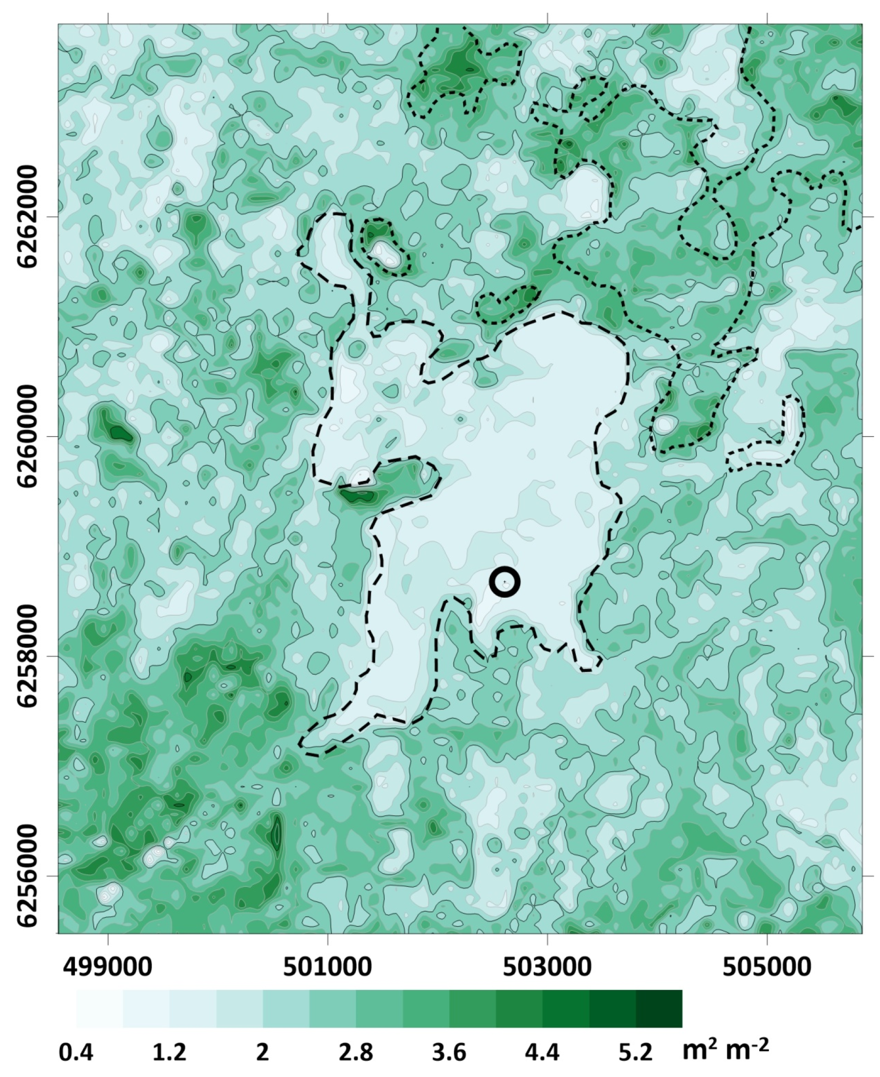
The selected modeling domain has an area of 60.6 km2 and covers the peatland, adjacent forest, and grassland landscapes (Figure 1 and Figure 2). The input vegetation parameters to run the three-dimensional hydrodynamic model were collected during several field campaigns and taken from remote sensing data analysis. The boundaries of different plant communities and plant canopy properties (e.g., species composition, plant height, length and width of tree crowns, availability and density of understorey, etc.) were obtained from field surveys. The Normalized Difference Vegetation Index (NDVI) from Landsat 8 was used to derive the spatial pattern of the Leaf Area Index (LAI) within the peatland and surrounding landscapes (Figure 2).
The horizontal model grid spacing is 60 m × 60 m. An uneven grid is used along the vertical axis with a minimum step of 0.09 m near the ground surface and a linearly growing step with height. The height of the computational domain is 1000 m, and the maximum step along the vertical axis is 58 m. Summer 2016 was selected for numerical experiments and the further validation of the modeled CO2 fluxes via the eddy covariance flux measurements. The selected period is characterized by a minimum number of gaps in meteorological and CO2 flux measurements. We also assumed in our model experiments that the biophysical properties of the vegetation would remain unchanged throughout the selected summer months.
The required input wind speed and wind direction at the upper boundary of the selected modeling domain for our numerical experiments were taken from the ERA5 reanalysis dataset (the fifth generation ECMWF atmospheric reanalysis of the global climate) [57]. Incoming solar radiation data were taken from meteorological measurements at the flux tower installed in the southern part of the peatland. The biophysical properties of the forest and peatland vegetation were determined during previous experimental studies in the CFBR or taken from the literature [40,58].
A numerical solution to the problem is carried out using the stable finite-difference schemes in two steps. First, the initial boundary value problem for the sub-model describing the spatial distribution of wind flow velocity and turbulent exchange coefficient is solved. The found spatial distributions of V ¯ and K are then used to calculate the concentrations of CO2 and its fluxes at different locations within the modeling domain (see Supplementary Materials S3). Depending on the domain used, the computation takes about 15 minutes to simulate the spatial wind distribution and 5 minutes to describe the spatial pattern of CO2 concentration on a single computer core (e.g., Intel CORE i5). The calculations were made for each day of summer 2016.
Comparisons of the modeled and measured CO2 fluxes were conducted for mid-summer 2016 using the eddy flux data measured at midday under well-developed turbulence and during periods without precipitation.
The Pearson correlation coefficient was used for estimating a linear correlation between the modeled and measured fluxes. A p-value less than 0.05 was used to quantify statistical significance.

3. Results and Discussion

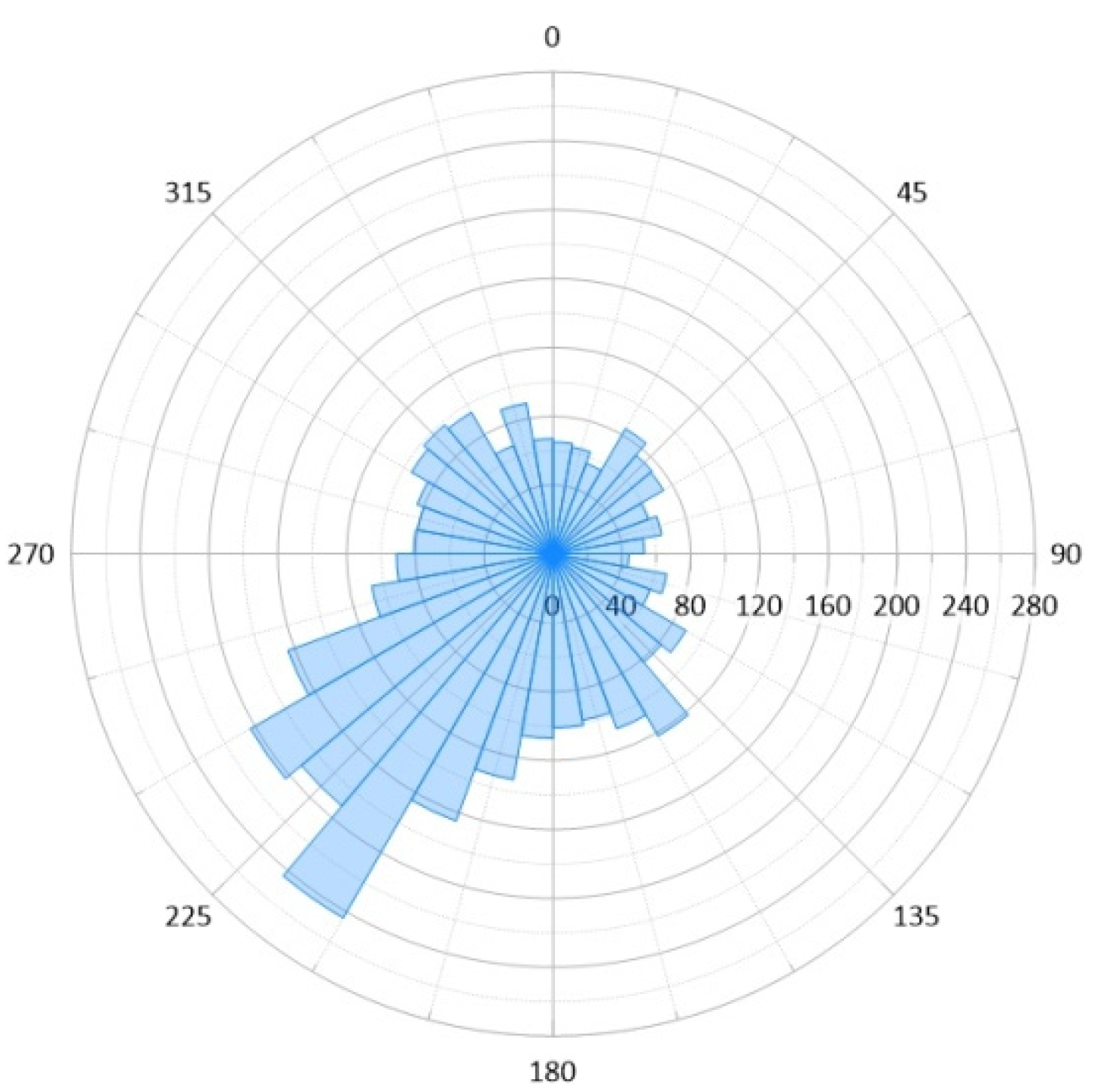
To illustrate the model’s capability to describe wind speed and CO2 flux distribution over the non-uniform forest peatland, we analyzed in more detail the numerical results for two selected days (25 June and 28 June 2016). The days are characterized by similar sunny weather conditions but different wind directions (southwestern and northwestern, respectively). Mostly sunny weather conditions and similar air temperatures on selected days have contributed to similar rates of soil respiration and plant photosynthesis. The southwest wind was the prevailing wind direction in the summer of 2016 (Figure 3). The northwest wind was less common (observed during polar air mass advection) and was chosen to quantify the possible effect of surrounding forest landscapes on the spatial patterns of CO2 fluxes within the study peatland.
Analysis of the spatial distribution of wind speed and turbulent kinetic energy patterns can reveal the possible disturbing effects of the surrounding forest canopy on the airflow pattern over the peatland, particularly on the air flows near the flux tower. We examined the robustness of model results on CO2 fluxes by comparing them with the eddy covariance CO2 flux measurements in the southern part of the peatland.

3.1. Spatial Distributions of Wind Speed and Turbulent Kinetic Energy within the Modeling Domain

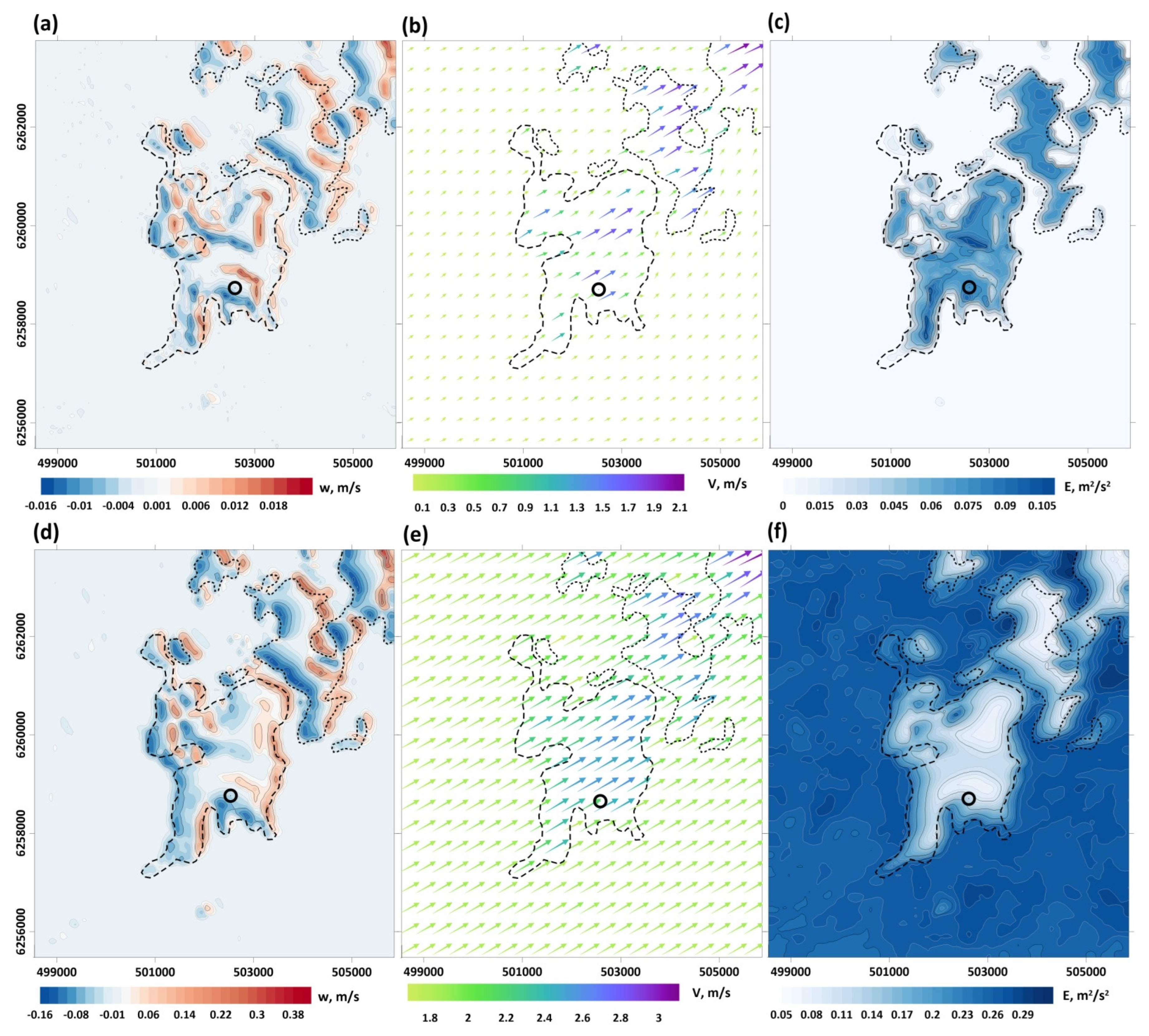
The results of the numerical experiments showed a substantial variability in wind speed and turbulence conditions within the modeling domain, mainly governed by the aerodynamic effects of different vegetation types of various heights and densities (Figure 4 and Figure 5). The maximum values of vertical velocity (Figure 4a,d and Figure 5a,d) were found on the leeward and the windward sides of the forest. Over tree crowns (30 m above the ground), they varied between −0.2 m s−1 on the leeward side and 0.6 m s−1 on the windward side (Figure 4d and Figure 5d). Near the ground surface (3 m above ground), the vertical velocities were slightly less (Figure 4a and Figure 5a). The horizontal flow velocity reached maximum values in open non-forested areas (peatland and abandoned grasslands in the northeastern part of the modeling domain). Sparse pine woody vegetation with a low leaf area index (see Figure 2) had no significant effect on vertical and horizontal flow velocities. Minor variability in flow velocity components was also detected within and above the forest with almost uniform vegetation structure, and over central parts of peatland and grassland areas free of woody vegetation. The area around the flux tower, situated away from forest edges and peatland woody undergrowth, was characterized by almost uniform wind speed distribution.
The weak reverse air flow characterizes the leeward sides of the peatland and openings (not shown). Similar but more intensive reverse air flows at the leeward forest side were detected in the experimental study conducted at the recently clear-cut area in the CFBR region [40]. The main differences between the results of our study and [40] are towing to different tree heights surrounding the peatland and the clear-cut and the presence of the dense shrub undergrowth at the forest edge around the peatland. Similar results were also obtained in several previous studies devoted to the effects of forest heterogeneity on spatial wind distribution [59,60,61,62].
The modeled distributions of TKE vary significantly at different heights within the peatland, surrounding forests, and grasslands. They are mainly caused by vegetation aerodynamic properties (Figure 4c,f and Figure 5c,f). Maximum TKEs are observed above the forest, whereas the TKE values over the peatland at the same level above the ground are generally lower. Local maximums of TKE above the forest are associated with the sites with sudden changes in vegetation density. In particular, such maximums are detected at windward forest edges of grasslands outside the peatland in the northeastern part of the modeling domain. An increase in TKE at the windward forest edge within the peatland area is not detected. That is because of a smooth change in LAI between the peatland and surrounding forest caused by the presence of dense shrubs and woody plants undergrowth at the forest edge.

3.2. Spatial Patterns of CO2 Fluxes within the Modeling Domain

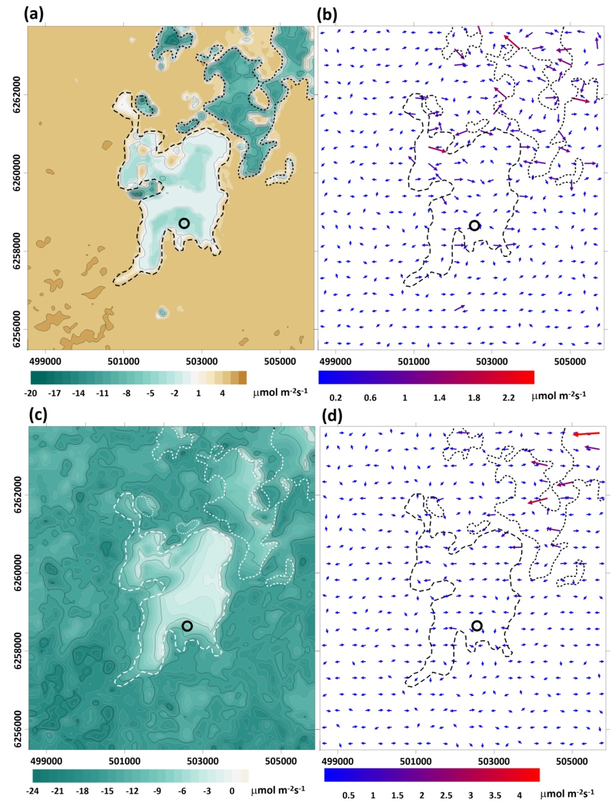
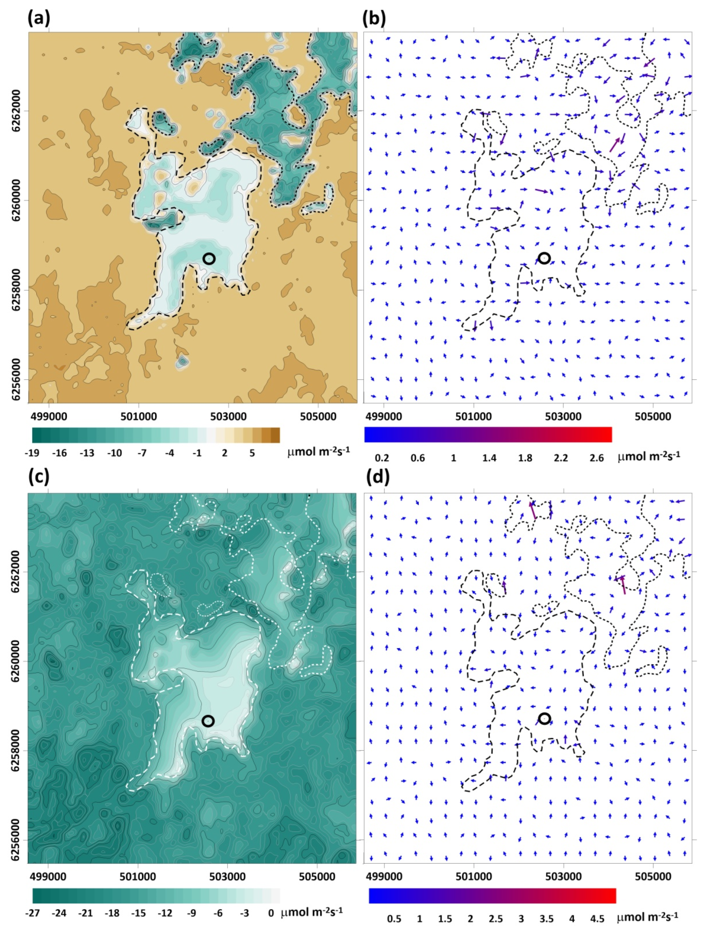
Figure 6 and Figure 7 show the spatial distributions of vertical and horizontal CO2 fluxes derived as the sum of turbulent and advective flux components at two heights (3 m and 30 m) above the ground surface. At the height of 3 m, almost all the area of the peatland serves as a sink of CO2 from the atmosphere (up to 5 μmol m−2 s−1) with local maxima in its northern and southern parts (Figure 6a and Figure 7a). The narrow peripheral zone of the peatland is a minor source of CO2 in the atmosphere. Near-ground CO2 fluxes inside the surrounding forest are almost positive (CO2 release into the atmosphere) due to the low rate of understorey photosynthesis and intensive soil respiration. The maximum CO2 uptake rates are observed at the abandoned grasslands in the northwestern part of the modeling domain (up to 19 µmol m−2 s−1 regardless of wind direction). Slight differences in the air temperature on 25 June 2016 (with a maximum of 24.8 °C at 14:00, Figure 6) and 28 June 2016 (with a maximum of 27.8 °C at 13:30, Figure 7) under similar solar radiation, air temperature and humidity conditions did not significantly affect CO2 fluxes over the peatland.
The horizontal CO2 fluxes within the modeling domain are relatively low and have maximum values at the boundaries of different vegetation types with different heights and densities (Figure 6b and Figure 7b). The full magnitude of the horizontal fluxes is about two times smaller than the maximum values of vertical fluxes at the peatland and up to eight times smaller than the maximum values of vertical fluxes within the entire modeling domain.
The spatial pattern of vertical and horizontal fluxes in mid-day under sunny summer weather conditions over the peatland at the height of 30 m shows a strongly non-uniform distribution. It depends on the prevailing wind direction and differs significantly from the spatial flux distributions at lower altitudes (Figure 6c,d and Figure 7c,d). Whereas at the height of 3 m over the peatland, the CO2 fluxes vary from −5 to 4 μmol m−2 s−1, at the height of 30 m, the CO2 fluxes are negative everywhere (CO2 uptake from the atmosphere), and range, depending on the wind direction, from −16 to 0 μmol m−2 s−1 (Figure 6c and Figure 7c). The maximum negative (downward) CO2 fluxes are detected in the northwestern and western parts of the peatland area. They can be explained by CO2 advection by airflow from the upwind forest side. Analysis of vertical fluxes shows that the surrounding forest has higher CO2 uptake rates than the peatland. Above the surrounding forest, the vertical CO2 fluxes vary between −12 and −26 μmol m−2 s−1, and the flux range is in good agreement with the vertical CO2 fluxes measured by the eddy covariance technique at the neighboring experimental forest site [45].
The horizontal CO2 fluxes within the peatland at the height of 30 m are somewhat higher than those at the height of 3 m and vary from 0.2 to 4.6 μmol m−2 s−1, with maxima at the forest edges with high horizontal LAI gradients (Figure 6d and Figure 7d). The magnitude of the horizontal fluxes within the peatland area is about ten times lower than the maximum values of vertical fluxes.

3.3. Comparison of the Model Simulation and Eddy Covariance CO2 Flux Measurements

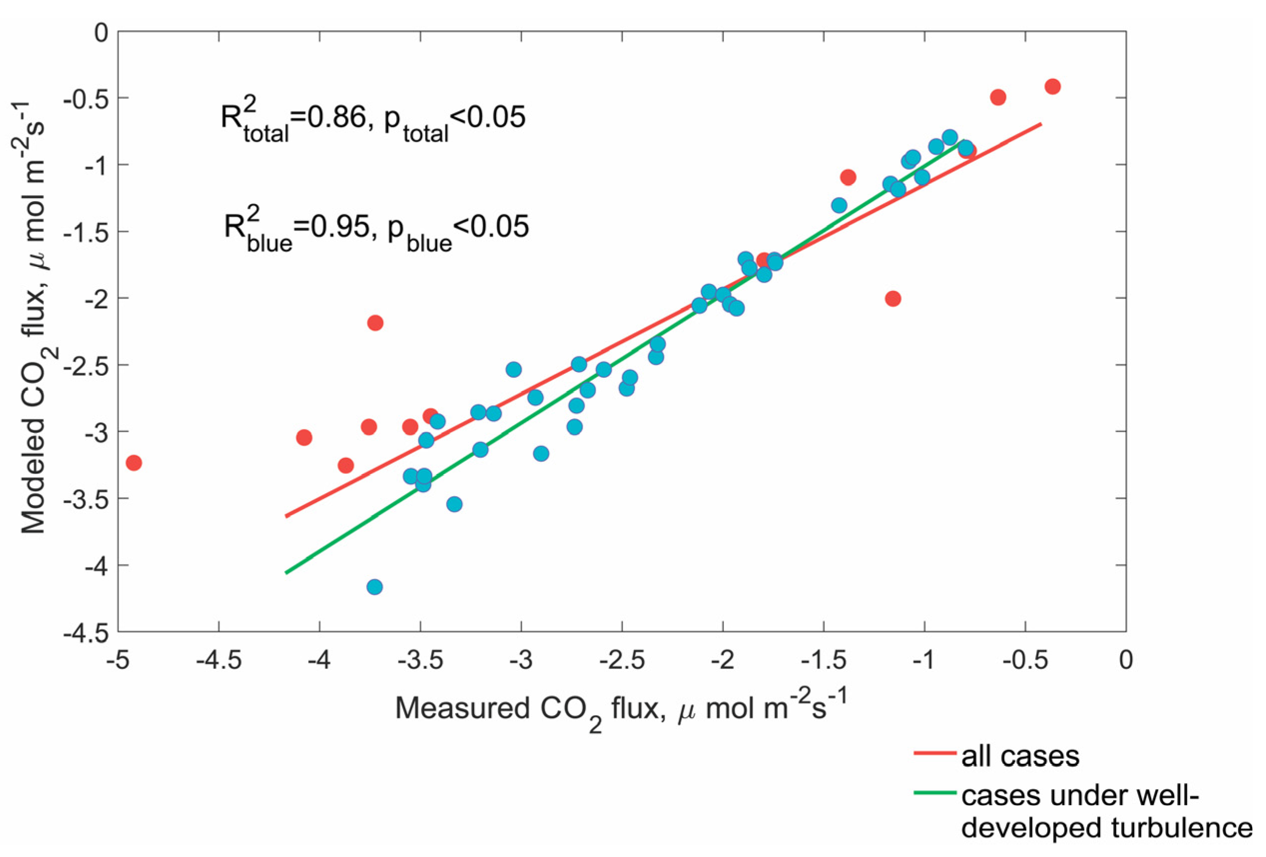
Comparisons of the modeled and measured vertical CO2 fluxes conducted for mid-summer 2016 show a good fit (Figure 8). Both modeled and measured vertical CO2 fluxes are primarily negative (i.e., directed to the surface), indicating that the peatland serves as a sink of CO2 from the atmosphere in the mid-day summertime. The R-squared (R2) value between the modeled and measured vertical turbulent fluxes was about 0.86 (p < 0.05). Excluding the cases of non-fully developed turbulence (u* < 0.05) and high air temperature (higher than 28 °C) results in an increase in the R2 value up to 0.95 (p < 0.05). Weak turbulence can be a reason for some CO2 flux underestimations [7]. Some differences between modeled and measured fluxes may also be related to the simplified parameterization of soil emissions that rely on soil temperature [11]. Several studies have analyzed possible uncertainties of the Arrhenius-type dependence on soil respiration under high soil (air) temperatures [63]. It was shown that the respiration rate could follow the Gaussian response, increasing with soil temperature up to some thresholds, above which the respiration rates decrease with further temperature rise. Overestimated ecosystem respiration due to high air temperatures may be a reason for lower predicted net CO2 uptakes in the mid-day hours in the peatland.
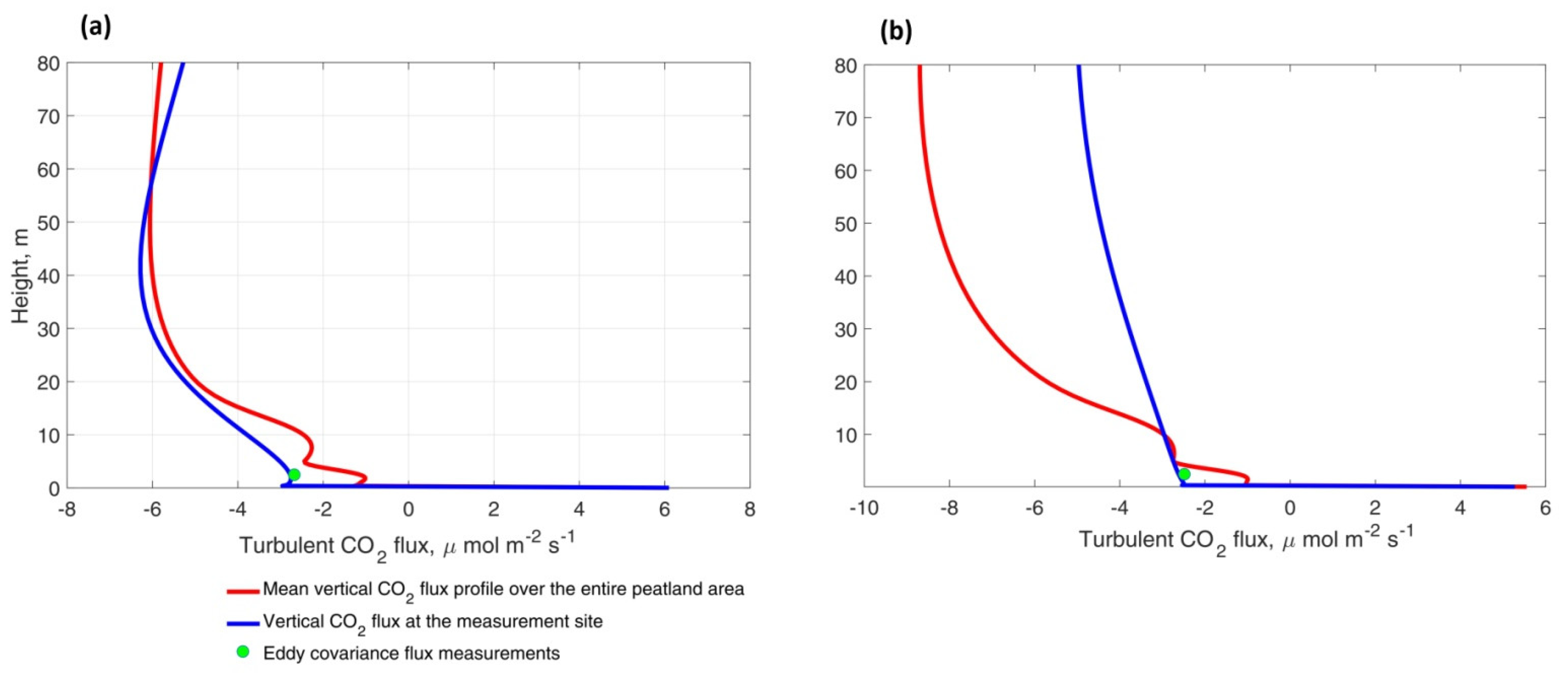
Comparisons of vertical profiles of CO2 fluxes at the eddy covariance measurement site and over the entire peatland area showed, on the one hand, a very strong vertical heterogeneity of the CO2 fluxes within the atmospheric surface layer and, on the other hand, the flux differences between the flux tower location and the entire peatland area (Figure 9).
The vegetation of the peatland is very mosaic, and it is represented by various moss and grass species. Some areas are covered by rare pine 1–5 m high. Plants of different species have different rates of photosynthesis and respiration. Soil respiration is also strongly spatially heterogeneous. All these factors result in the averaged CO2 flux over the whole peatland space being slightly lower near the ground surface (lower CO2 uptake) than the corresponding flux at the measuring tower location (Figure 9).
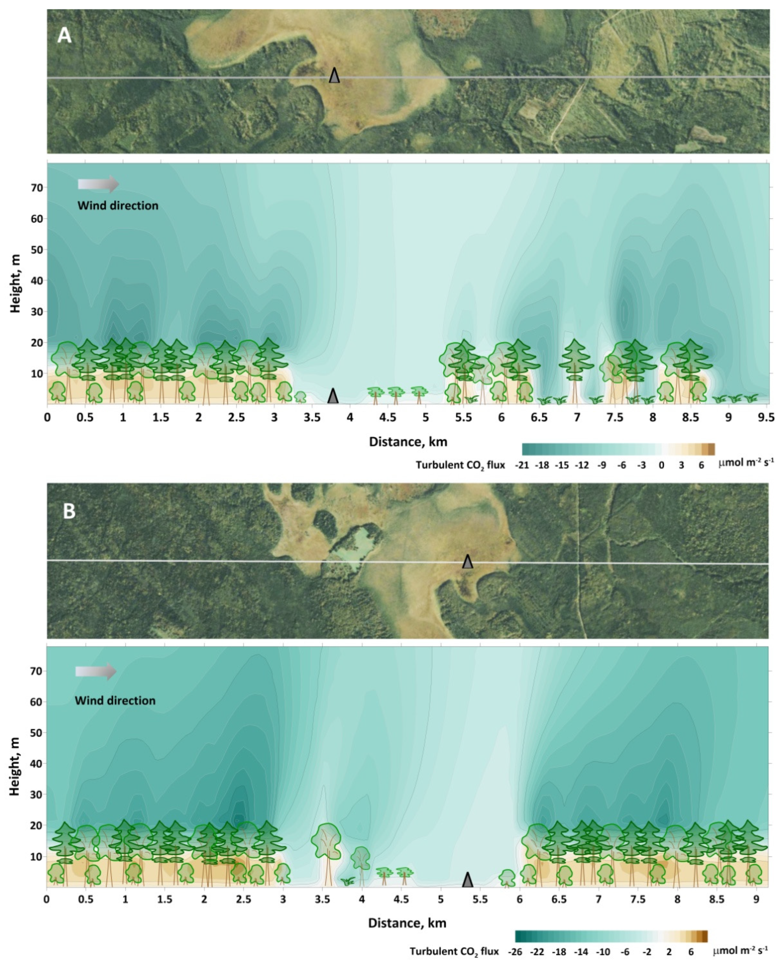
The flux growth with height increase is probably due to CO2 advection by the airflow from surrounding forests which are characterized by much higher photosynthesis and CO2 uptake rates (Figure 10). The difference between the vertical profiles of CO2 fluxes on different days is mainly caused by the various distances between the eddy covariance measurement site and forest border, which pass the air mass over the peatland under different wind directions (Figure 10).
The local extremes of the mean CO2 flux over the entire peatland (the red lines in Figure 9a,b) at 5 m above the surface can be explained by the presence of pine-covered patches in the peatland. Because of photosynthesis, the absorption of CO2 over these patches is enhanced inside the canopy space. At the same time, the photosynthesis rate of understory vegetation is reduced due to shading caused by the presence of trees [64].
Analysis of the sensitivity of the simulation results to the used value of parameter Cμ showed that despite the significant effect on the spatial pattern of the turbulent exchange coefficient, the choice of Cμ value has no considerable impact on modeled CO2 fluxes in the case of flat terrain. Numerical experiments showed that 50% changes in Cμ resulted in only 6% changes in vertical turbulent CO2 fluxes and 9% changes in advective CO2 fluxes (although the absolute value is two orders of magnitude less than the turbulent one) in the central parts of the peatland (see Supplementary Materials S4).

4. Conclusions

A 3D hydrodynamic model of the atmospheric boundary layer was developed. Despite the use of simplifications, the present version of the model has demonstrated an ability to reasonably describe the spatial distribution of the air flows above the spatially non-uniform ombrotrophic Staroselsky Moch peatland in the central part of European Russia. Airflow simulations showed significant heterogeneity in the wind distributions within the atmospheric surface layer over the peatland and surrounding forest and grasslands. As expected, the most pronounced changes in vertical and horizontal wind components were found at the windward and leeward forest edges.
Comparing the modeled fluxes for the central parts of the peatland with eddy covariance flux measurements showed their good agreement. The R-squared value between the modeled and measured vertical turbulent fluxes was about 0.86 (p < 0.05). Excluding the cases of non-fully developed turbulence (u* < 0.05) and high air temperature (higher 28 °C) resulted in an increase in the R2 value up to 0.95 (p < 0.05).
The heterogeneity of the vegetation cover within the peatland and the surrounding landscapes leads to a very uneven distribution of the CO2 flux over the modeling domain. The simulated or measured local vertical CO2 fluxes (e.g., by eddy covariance technique) at some sites within the peatland differed from the mean CO2 fluxes derived for the entire peatland area. The flux differences depend on the height above the ground, the distance from the forest edge, and vegetation properties in the upwind direction.
In addition, an analysis of the model sensitivity to the model constants used (particularly to the dimensionless numerical parameter Cμ that is used to describe the turbulent exchange coefficient) was performed. This analysis showed that, despite the significant effect of Cμ on the spatial pattern of the turbulent exchange coefficient, its value does not have a considerable impact on the modeled CO2 fluxes over flat terrain.
Overall, it can be concluded that such 3D models are an effective tool for CO2 flux up-scaling over non-uniform landscapes. Because of the simplicity of input parameters for model initialization and low computing cost, the model can be applied as a practical tool to evaluate the environmental effects of heterogeneous landscapes with mosaic vegetation and non-uniform distribution patterns of soil resources (e.g., carbon, water, nutrients) on vertical CO2 fluxes, not only on specific locations but over extensive areas of interest. It can be applied in a number of ecological tasks, including GHG flux up-scaling from local to regional scale, estimation of the non-linear effects of different forest management practices and forest disturbances on GHG uptake and release into the atmosphere, and retrieval of the GHG fluxes from remote sensing data including satellite and UAV (unmanned aerial vehicle) observations. To better meet these challenges, the presented model will be improved by using more complex parameterizations for some biophysical processes in plant canopy and soil.

Supplementary Materials

The following supporting information can be downloaded at: https://www.mdpi.com/article/10.3390/atmos14040625/s1. S1: Initial and boundary conditions for the dynamical part of the model. S2: Initial and boundary conditions for CO2 exchange for the dynamical part of the model. S3: Numerical solution of the differential equations. S4: Sensitivity of spatial wind and turbulence patterns to Cμ changes.

Author Contributions

Conceptualization, A.O. and I.M.; methodology, A.O., A.S. and I.M.; software, I.M.; validation, I.M.; formal analysis, I.M.; investigation, I.M., R.G. and A.O.; resources, J.K.; data curation, J.K.; data analysis, D.T. and R.G.; writing—original draft preparation, I.M.; writing—review and editing, A.O., A.S. and I.M.; visualization, I.M., A.O.; supervision, A.O.; project administration, A.O.; funding acquisition, A.O. All authors have read and agreed to the published version of the manuscript.

Funding

The modeling study conducted by I. Mukhartova was supported by Lomonosov Moscow State University (grant number AAAA-A16-116032810086-4) and performed within the Development program of the Interdisciplinary Scientific and Educational School of M.V. Lomonosov Moscow State University “Future Planet and Global Environmental Change”. A. Sogachev was supported by the state assignment FFER-2022-0002.

Institutional Review Board Statement

Not applicable.

Informed Consent Statement

Not applicable.

Data Availability Statement

The data obtained in the study can be requested from the authors at [email protected].

Acknowledgments

The authors express their sincere acknowledgment to Viktor M. Stepanenko for valuable comments and recommendations when writing the article.

Conflicts of Interest

The authors declare no conflict of interest.

References

  1. Pörtner, H.-O.; Roberts, D.C.; Tignor, M.; Poloczanska, E.S.; Mintenbeck, K.; Alegría, A.; Craig, M.; Langsdorf, S.; Löschke, S.; Möller, V.; et al. (Eds.) IPCC, 2022: Climate Change 2022: Impacts, Adaptation, and Vulnerability; Contribution of Working Group II to the Sixth Assessment Report of the Intergovernmental Panel on Climate Change; Cambridge University Press: Cambridge, UK; New York, NY, USA, 2022; 3056p. [Google Scholar]
  2. Yue, X.-L.; Gao, Q.-X. Contributions of natural systems and human activity to greenhouse gas emissions. Adv. Clim. Change Res. 2018, 9, 243–252. [Google Scholar] [CrossRef]
  3. Dong, F.; Qin, C.; Zhang, X.; Zhao, X.; Pan, Y.; Gao, Y.; Zhu, J.; Li, Y. Towards Carbon Neutrality: The Impact of Renewable Energy Development on Carbon Emission Efficiency. Int. J. Environ. Res. Public Health 2021, 18, 13284. [Google Scholar] [CrossRef] [PubMed]
  4. Bonan, G.B. Forests and climate change: Forcings, feedbacks, and the climate benefits of forests. Science 2008, 320, 1444–1449. [Google Scholar] [CrossRef] [PubMed] [Green Version]
  5. Friedlingstein, P.; O’Sullivan, M.; Jones, M.W.; Andrew, R.M.; Gregor, L.; Hauck, J.; Le Quéré, C.; Luijkx, I.T.; Olsen, A.; Peters, G.P.; et al. Global Carbon Budget. Earth Syst. Sci. Data 2022, 14, 4811–4900. [Google Scholar] [CrossRef]
  6. Khalil, K.; Mary, B.; Renault, P. Nitrous oxide production by nitrification and denitrification in soil aggregates as affected by O2 concentration. Soil Biol. Biochem. 2004, 36, 687–699. [Google Scholar] [CrossRef]
  7. Aubinet, M.; Vesala, T.; Papale, D. Eddy Covariance: A Practical Guide to Measurement and Data Analysis; Springer: Dordrecht, The Netherlands, 2012; p. 438. [Google Scholar]
  8. Pumpanen, J.; Kolari, P.; Ilvesniemi, H.; Minkkinen, K.; Vesala, T.; Niinisto, S.; Lohila, A.; Larmola, T.; Morero, M.; Pihlatie, M.; et al. Comparison of different chamber techniques for measuring soil CO2 efflux. Agric. For. Meteorol. 2004, 123, 159–176. [Google Scholar] [CrossRef]
  9. Foken, T. The energy balance closure problem: An overview. Ecol. Appl. 2008, 18, 1351–1367. [Google Scholar] [CrossRef]
  10. Sogachev, A.; Panferov, O.; Ahrends, B.; Doering, C.; Jørgensen, H.E. Numerical assessment of the effect of forest structure changes on CO2 flux footprints for the flux tower in Solling, Germany. Agric. For. Meteorol. 2011, 151, 746–754. [Google Scholar] [CrossRef]
  11. Vesala, T.; Huotari, J.; Rannik, Ü.; Suni, T.; Smolander, S.; Sogachev, A.; Launiainen, S.; Ojala, A. Eddy covariance measurements of carbon exchange and latent and sensible heat fluxes over a boreal lake for a full open-water period. J. Geophys. Res. Atmos. 2006, 111, D11101. [Google Scholar] [CrossRef]
  12. Sellers, P.; Dickinson, R.E.; Randall, D.A.; Betts, A.K.; Hall, F.G.; Berry, J.A.; Collatz, G.J.; Denning, A.S.; Mooney, H.A.; Nobre, C.A.; et al. Modeling the exchanges of energy, water, and carbon between continents and the atmosphere. Science 1997, 275, 502–509. [Google Scholar] [CrossRef] [Green Version]
  13. Vager, B.; Nadezhina, E. Atmospheric Boundary Layer in Conditions of Horizontal Non-Uniformity; Gidrometeoizdat: Leningrad, Russia, 1979. (In Russian) [Google Scholar]
  14. Penenko, V.; Aloyan, A. Models and Methods for Environmental Protection Problems; Science Publications: Moscow, Russia, 1985. (In Russian) [Google Scholar]
  15. Sogachev, A.; Panferov, O. Modification of two-equation models to account for plant drug. Bound. Layer Meteorol. 2006, 121, 229–266. [Google Scholar] [CrossRef]
  16. Sullivan, P.P.; McWilliams, J.C.; Moeng, C.-H. A subgrid-scale model for large-eddy simulation of planetary boundary-layer flows. Bound. Layer Meteorol. 1994, 71, 247–276. [Google Scholar] [CrossRef] [Green Version]
  17. Warner, T.T. Numerical Weather and Climate Prediction; Cambridge University Press: Cambridge, UK, 2011. [Google Scholar]
  18. Stull, R.B. An introduction to Boundary Layer Meteorology; Kluwer Academic Publishers: Dordrecht, The Netherlands, 1988. [Google Scholar] [CrossRef]
  19. Garrat, J. The Atmospheric Boundary Layer; Cambridge University Press: Cambridge, UK, 1992. [Google Scholar]
  20. Wyngaard, J.C. Turbulence in the Atmosphere; Cambridge University Press: Cambridge, UK, 2010. [Google Scholar]
  21. Raupach, M.R.; Finnigan, J.J. Single-layer models of evaporation from plant canopy are incorrect but useful, whereas multilayer models are correct but useless: Discuss. Aust. J. Plant Physiol. 1988, 15, 705–716. [Google Scholar] [CrossRef]
  22. Olchev, A.; Radler, K.; Sogachev, A.; Panferov, O.; Gravenhorst, G. Application of a three-dimensional model for assessing effects of small clear-cuttings on radiation and soil temperature. Ecol. Model. 2009, 220, 3046–3056. [Google Scholar] [CrossRef]
  23. Payne, R.J.; Malysheva, E.; Tsyganov, A.; Pampura, T.; Novenko, E.; Volkova, E.; Babeshko, K.; Mazei, Y. A multi-proxy record of Holocene environmental change, peatland development and carbon accumulation from Staroselsky Moch peatland, Russia. Holocene 2016, 26, 314–326. [Google Scholar] [CrossRef]
  24. Peel, M.C.; Finlayson, B.L.; McMahon, T.A. Updated world map of the Koppen-Geiger climate classification. Hydrol. Earth Syst. Sci. 2007, 11, 1633–1644. [Google Scholar] [CrossRef] [Green Version]
  25. Novenko, E.Y.; Olchev, A.V. Early Holocene vegetation and climate dynamics in the central part of the East European Plain (Russia). Quat. Int. 2015, 388, 12–22. [Google Scholar] [CrossRef]
  26. Papale, D.; Reichstein, M.; Aubinet, M.; Canfora, E.; Bernhofer, C.; Kutsch, W.; Longdoz, B.; Rambal, S.; Valentini, R.; Vesala, T.; et al. Towards a standardized processing of Net Ecosystem Exchange measured with eddy covariance technique: Algorithms and uncertainty estimation. Biogeosciences 2006, 3, 571–583. [Google Scholar] [CrossRef] [Green Version]
  27. Kljun, N.; Calanca, P.; Rotach, M.W.; Schmid, H.P. A simple parameterization for flux footprint predictions. Bound. Layer Meteorol. 2004, 112, 503–523. [Google Scholar] [CrossRef]
  28. Dubov, A.S.; Bykova, L.P.; Marunich, S.V. Turbulence in Vegetation Canopy; Gidrometeoizdat: Leningrad, Russia, 1978. (In Russian) [Google Scholar]
  29. Sogachev, A.; Menzhulin, G.V.; Heimann, M.; Lloyd, J. A simple three-dimensional canopy-planetary boundary layer simulation model for scalar concentrations and fluxes. Tellus 2002, 54B, 784–819. [Google Scholar]
  30. Sorbjan, Z. Structure of the Atmospheric Boundary Layer; Prentice-Hall: Englewood Cliffs, NJ, USA, 1989. [Google Scholar]
  31. Katul, G.G.; Mahrt, L.; Poggi, D.; Sanz, C. One- and two-equation models for canopy turbulence. Bound. Layer Meteorol. 2004, 113, 81–109. [Google Scholar] [CrossRef] [Green Version]
  32. Mamkin, V.V.; Mukhartova, Y.V.; Diachenko, M.S.; Kurbatova, J.A. Three-year variability of energy and carbon dioxide fluxes at clear-cut forest site in the European Southern Taiga. Geogr. Environ. Sustain. 2019, 1, 197–212. [Google Scholar] [CrossRef] [Green Version]
  33. Olchev, A.V.; Mukhartova, Y.V.; Levashova, N.T.; Volkova, E.M.; Ryzhova, M.S.; Mangura, P.A. The influence of the spatial heterogeneity of vegetation cover and surface topography on vertical CO2 fluxes within the atmospheric surface layer. Izv. Atmos. Ocean. Phys. 2017, 53, 539–549. [Google Scholar] [CrossRef]
  34. Sanz, C. A note on k-ε modelling of vegetation canopy airflows. Bound. Layer Meteorol. 2003, 108, 191–197. [Google Scholar] [CrossRef]
  35. Pope, S.B. Turbulent Flows; Cambridge University Press: Cambridge, UK, 2000. [Google Scholar]
  36. Wilcox, D.C. Turbulence Modeling for CFD; DCW Industries, Inc.: La Canada, CA, USA, 1998. [Google Scholar]
  37. Kolmogorov, A. Turbulence flow equations of an uncompressible fluid. Trans. USSR Acad. Sci. Book Phys. 1942, 6, 56–58. [Google Scholar]
  38. Seginer, I.; Mulhearn, P.J.; Bradley, E.F.; Finnigan, J.J. Turbulent flow in a model plant canopy. Bound. Layer Meteorol. 1976, 10, 423–453. [Google Scholar] [CrossRef]
  39. Sogachev, A. A Note on Two-Equation Closure Modelling of Canopy Flow. Bound. Layer Meteorol. 2009, 130, 423–435. [Google Scholar] [CrossRef]
  40. Mamkin, V.; Kurbatova, J.; Avilov, V.; Mukhartova, Y.; Krupenko, A.; Ivanov, D.; Levashova, N.; Olchev, A. Changes in net ecosystem exchange of CO2, latent and sensible heat fluxes in a recently clear-cut spruce forest in western Russia: Results from an experimental and modeling analysis. Environ. Res. Lett. 2016, 11, 125012. [Google Scholar] [CrossRef]
  41. Mukhartova, Y.V.; Dyachenko, M.S.; Mangura, P.A.; Mamkin, V.V.; Kurbatova, J.A.; Olchev, A.V. Application of a three-dimensional model to assess the effect of clear-cutting on carbon dioxide exchange at the soil-vegetation-atmosphere interface. IOP Conf. Ser. Earth Environ. Sci. 2019, 368, 012036. [Google Scholar] [CrossRef]
  42. Mukhartova, Y.V.; Mangura, P.A.; Levashova, N.T.; Olchev, A.V. Selection of boundary conditions for modeling the turbulent exchange process within the atmospheric surface layer. Comput. Res. Model. 2018, 10, 27–46. (In Russian) [Google Scholar] [CrossRef] [Green Version]
  43. Chen, H.; Sun, S.; Zhang, T. Energy Stability Analysis of Some Fully Discrete Numerical Schemes for Incompressible Navier-Stokes Equations on Staggered Grids. J. Sci. Comput. 2018, 75, 427–456. [Google Scholar] [CrossRef]
  44. Belotserkovskiy, O.M. Numerical Modeling in Continuum Mechanics; Fiziko-Matematicheskaya Literatura: Moscow, Russia, 1994. (In Russian) [Google Scholar]
  45. Mamkin, V.; Kurbatova, J.; Avilov, V.; Ivanov, D.; Kuricheva, O.; Varlagin, A.; Yaseneva, I.; Olchev, A. Energy and CO2 exchange in an undisturbed spruce forest and clear-cut in the Southern Taiga. Agric. For. Meteorol. 2019, 265, 252–268. [Google Scholar] [CrossRef]
  46. Belov, A.A.; Kalitkin, N.N. Evolutionary factorization and superfast relaxation count. Math. Model. Comput. Simul. 2015, 7, 103–116. [Google Scholar] [CrossRef]
  47. Belov, A.A.; Kalitkin, N.N.; Kuzmina, L.V. Modeling of chemical kinetics in gases. Math. Model. Comput. Simul. 2017, 9, 24–39. [Google Scholar] [CrossRef]
  48. Mukhartova, Y.; Postylyakov, O.; Davydova, M.; Zakharova, S. High-detailed tropospheric transport of NOx from ground sources: Comparison of model data and satellite imagery. In Proceedings of the Remote Sensing of Clouds and the Atmosphere XXVI, Online, 13–17 September 2021; p. 1185906. [Google Scholar]
  49. Flesch, T.K.; Prueger, J.H.; Hatfield, J.L. Turbulent Schmidt number from a tracer experiment. Agric. For. Meteorol. 2002, 111, 299–307. [Google Scholar] [CrossRef]
  50. Ball, J.T.; Woodrow, I.E.; Berry, J.A. A Model Predicting Stomatal Conductance and its Contribution to the Control of Photosynthesis under Different Environmental Conditions. In Progress in Photosynthesis Research; Springer: Dordrecht, The Netherlands, 1987; pp. 221–224. [Google Scholar]
  51. Leuning, R. A critical appraisal of a combined stomatal-photosynthesis model for C3 plants. Plant Cell Environ. 1995, 18, 339–355. [Google Scholar] [CrossRef]
  52. Oltchev, A.; Ibrom, A.; Constantin, J.; Falk, M.; Richter, I.; Morgenstern, K.; Joo, Y.; Kreilein, H.; Gravenhorst, G. Stomatal and surface conductance of a spruce forest: Model simulation and field measurements. J. Phys. Chem. Earth 1998, 23, 453–458. [Google Scholar] [CrossRef]
  53. Lloyd, J.; Taylor, J.A. On the temperature dependence of soil respiration. Funct. Ecol. 1994, 8, 315–323. [Google Scholar] [CrossRef]
  54. Blanken, P.D.; Williams, M.W.; Burns, S.P.; Monson, R.K.; Knowles, J.; Chowanski, K.; Ackerman, T. A comparison of water and carbon dioxide exchange at a windy alpine tundra and subalpine forest site near Niwot Ridge, Colorado. Biogeochemistry 2009, 95, 61–76. [Google Scholar] [CrossRef]
  55. Feigenwinter, C.; Bernhofer, C.; Eichelmann, U.; Heinesch, B.; Hertel, M.; Janous, D.; Kolle, O.; Lagergren, F.; Lindroth, A.; Minerbi, S.; et al. Comparison of horizontal and vertical advective CO2 fluxes at three forest sites. Agric. For. Meteorol. 2008, 148, 12–24. [Google Scholar] [CrossRef]
  56. Leuning, R.; Zegelin, S.J.; Jones, K.; Keith, H.; Hughes, D. Measurement of horizontal and vertical advection of CO2 within a forest canopy. Agric. For. Meteorol. 2008, 148, 1777–1797. [Google Scholar] [CrossRef] [Green Version]
  57. Hersbach, H.; Bell, B.; Berrisford, P.; Hirahara, S.; Horányi, A.; Muñoz-Sabater, J.; Nicolas, J.; Peubey, C.; Radu, R.; Schepers, D.; et al. The ERA5 Global Reanalysis. Q. J. R. Meteorol. Soc. 2020, 146, 1999–2049. [Google Scholar] [CrossRef]
  58. Kurbatova, J.; Li, C.; Varlagin, A.; Xiao, X.; Vygodskaya, N. Modeling carbon dynamics in two adjacent spruce forests with different soil conditions in Russia. Biogeosciences 2008, 5, 969–980. [Google Scholar] [CrossRef] [Green Version]
  59. Belcher, S.E.; Finnigan, J.J.; Harman, I.N. Flows through forest canopies in complex terrain. Ecol. Appl. 2008, 18, 1436–1453. [Google Scholar] [CrossRef]
  60. Detto, M.; Katul, G.G.; Siqueira, M.; Juang, J.H.; Stoy, P.C. The structure of turbulence near a tall forest edge: The backward facing step flow analogy revisited. Ecol. Appl. 2008, 18, 1420–1435. [Google Scholar] [CrossRef] [Green Version]
  61. Panferov, O.; Sogachev, A. Influence of gap size on wind damage variables in a forest. Agric. For. Meteorol. 2008, 148, 1869–1881. [Google Scholar] [CrossRef]
  62. An, L.; Wang, J.; Xiong, N.; Wang, Y.; You, J.; Li, H. Assessment of permeability windbreak forests with different porosities based on laser scanning and computational fluid dynamics. Remote Sens. 2022, 14, 3331. [Google Scholar] [CrossRef]
  63. Carey, J.C.; Tang, J.; Templer, P.H.; Kroeger, K.D.; Crowther, T.W.; Burton, A.J.; Dukes, J.S.; Emmett, B.; Frey, S.D.; Heskel, M.A.; et al. Temperature response of soil respiration largely unaltered with experimental warming. Proc. Natl. Acad. Sci. USA 2016, 113, 13797–13802. [Google Scholar] [CrossRef] [PubMed] [Green Version]
  64. Pridacha, V.B.; Sazonova, T.A.; Novichonok, E.V.; Semin, D.E.; Tkachenko, Y.N.; Pekkoev, A.N.; Timofeeva, V.V.; Bakhmet, O.N.; Olchev, A.V. Clear-cutting impacts nutrient, carbon and water exchange parameters in woody plants in an east Fennoscandian pine forest. Plant Soil 2021, 466, 317–336. [Google Scholar] [CrossRef]
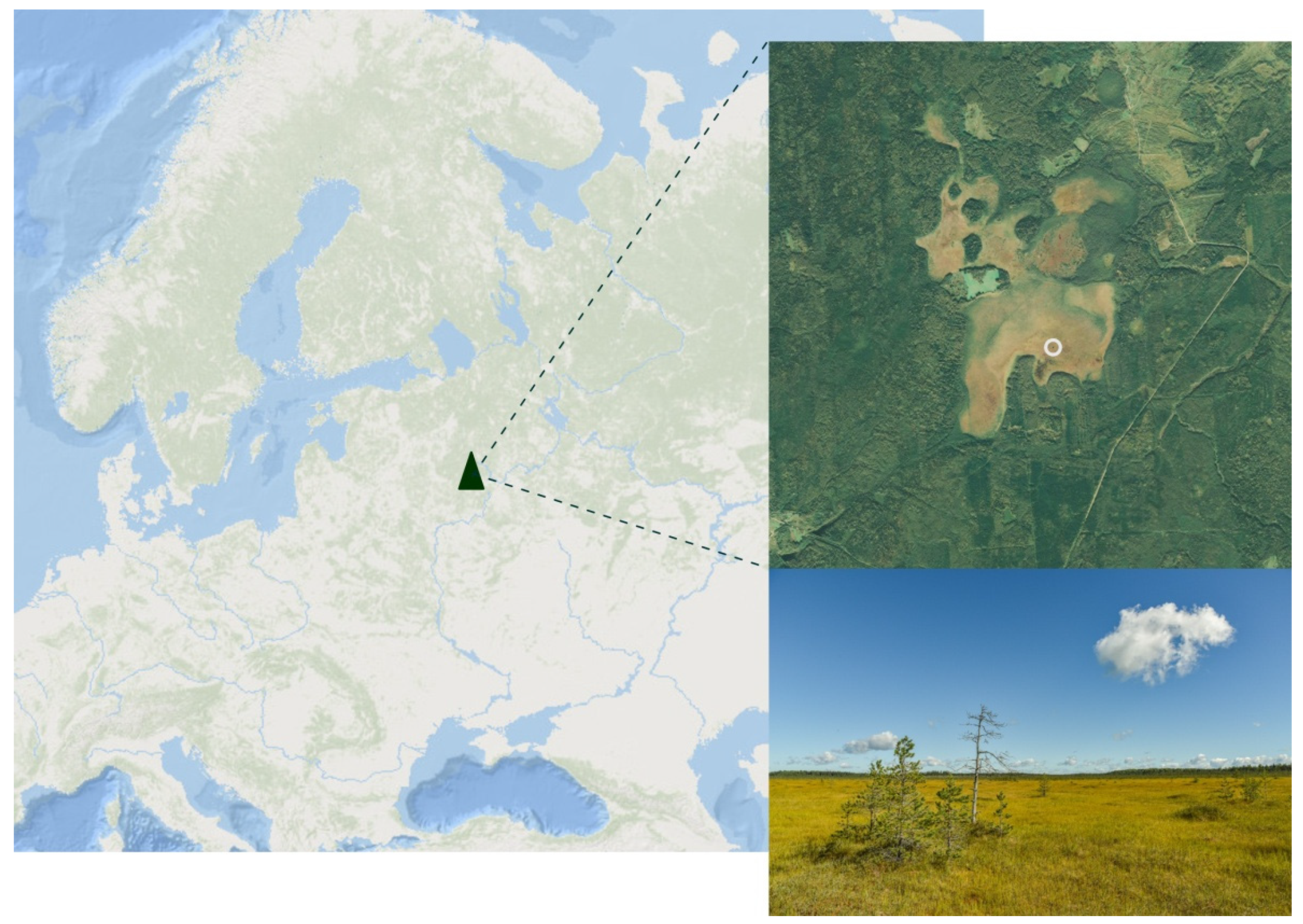
Figure 1. Geographical location, satellite image, and photo of the study area. The white circle indicates the location of the eddy covariance flux station.
Atmosphere 14 00625 g001
Figure 2. Spatial pattern of the leaf area index (LAI) for the selected modeling domain covering the Staroselsky Moch peatland and surrounding landscapes. The medium-dashed line shows the peatland boundary. The short-dashed line shows the boundaries of abandoned lands with grassy vegetation and open places. The black circle indicates the location of the eddy covariance flux station. The coordinate system is Universal Transverse Mercator (UTM, 36N).
Atmosphere 14 00625 g002
Figure 3. The wind speed and direction distribution (wind rose) at the Staroselsky Moch peatland in the summer of 2016.
Atmosphere 14 00625 g003
Figure 4. Modeled vertical (a,d) and horizontal (b,e) flow velocity, and turbulent kinetic energy (c,f) distributions at the heights of 3 (ac) and 30 (df) m above the ground. Calculations were performed using meteorological data at 14:00 on 25 June 2016. The wind direction at the upper boundary of the modeling domain is southwest. The medium-dashed line shows the peatland boundary. The short-dashed line shows the boundaries of abandoned lands with grassy vegetation and open places. The black circle indicates the location of the eddy covariance flux station. The negative vertical flow component corresponds to the downward air flows, and positive, to the upward ones. The coordinate system is Universal Transverse Mercator (UTM, 36N).
Atmosphere 14 00625 g004
Figure 5. Modeled vertical (a,d) and horizontal (b,e) flow velocity, and turbulent kinetic energy (c,f) distributions at the heights of 3 (ac) and 30 (df) m above the ground. Calculations were performed using meteorological data at 13:30 on 28 June 2016. The wind direction at the upper boundary of the modeling domain is northwest. The medium-dashed line shows the peatland boundary. The short-dashed line shows the boundaries of abandoned lands with grassy vegetation and open places. The black circle indicates the location of the eddy covariance flux station. Negative vertical flow component corresponds to the downward air flows, and positive to the upward ones. Coordinate system is Universal Transverse Mercator (UTM, 36N).
Atmosphere 14 00625 g005
Figure 6. Modeled vertical (a,c) and horizontal (b,d) CO2 fluxes (turbulent and advective) at the heights of 3 (a,b) and 30 (c,d) m above the ground. Calculations were performed using meteorological data at 14:00 on 25 June 2016. The medium-dashed line shows the peatland boundary. The short-dashed line shows the boundaries of abandoned lands with grassy vegetation and open places. The black circle indicates the location of the eddy covariance flux station. The coordinate system is Universal Transverse Mercator (UTM, 36N).
Atmosphere 14 00625 g006
Figure 7. Modeled vertical (a,c) and horizontal (b,d) CO2 fluxes (turbulent and advective) at the heights of 3 (a,b) and 30 (c,d) m above the ground. Calculations were performed using meteorological data at 13:03 on 28 June 2016. The medium-dashed line shows the peatland boundary. The short-dashed line shows the boundaries of abandoned lands with grassy vegetation and open places. The black circle indicates the location of the eddy covariance flux station. The coordinate system is Universal Transverse Mercator (UTM, 36N).
Atmosphere 14 00625 g007
Figure 8. Comparisons of vertical CO2 fluxes simulated by 3D model and measured by the eddy covariance technique for summer 2016. Blue points show the cases of flux measurements under well-developed turbulence and air temperatures below 28 °C. Red points show measured fluxes under friction velocity lower than 0.05 m s−1 or in the case of air temperatures, above 28 °C. The red line is the linear regression for all cases (R2 = 0.86, p < 0.05). The green line is the linear regression for the blue points (R2 = 0.95, p < 0.05).
Atmosphere 14 00625 g008
Figure 9. Modeled vertical profiles: CO2 fluxes at the eddy covariance measurement site in the southern part of the peatland and average CO2 fluxes over the entire peatland area under (a) southwest (25 June 2016 at 14:00) and (b) northwest wind directions (28 June 2016 at 13:30). Green points indicate the eddy covariance flux measurements at the height of 2 m above the ground.
Atmosphere 14 00625 g009
Figure 10. Top views and modeled cross-sections of vertical CO2 fluxes along the two directions that cross the peatland and pass through the flux measurement site: (A) 25 June 2016 at 14:00, (B) 28 June 2016 at 13:30. The grey triangle indicates the location of the eddy covariance flux station. White lines in the top views indicate the locations of the cross-sections.
Atmosphere 14 00625 g010
Disclaimer/Publisher’s Note: The statements, opinions and data contained in all publications are solely those of the individual author(s) and contributor(s) and not of MDPI and/or the editor(s). MDPI and/or the editor(s) disclaim responsibility for any injury to people or property resulting from any ideas, methods, instructions or products referred to in the content.