
Research on Missing Value Imputation to Improve the Validity of Air Quality Data Evaluation on the Qinghai-Tibetan Plateau

 , ,
, ,
Abstract
:1. Introduction
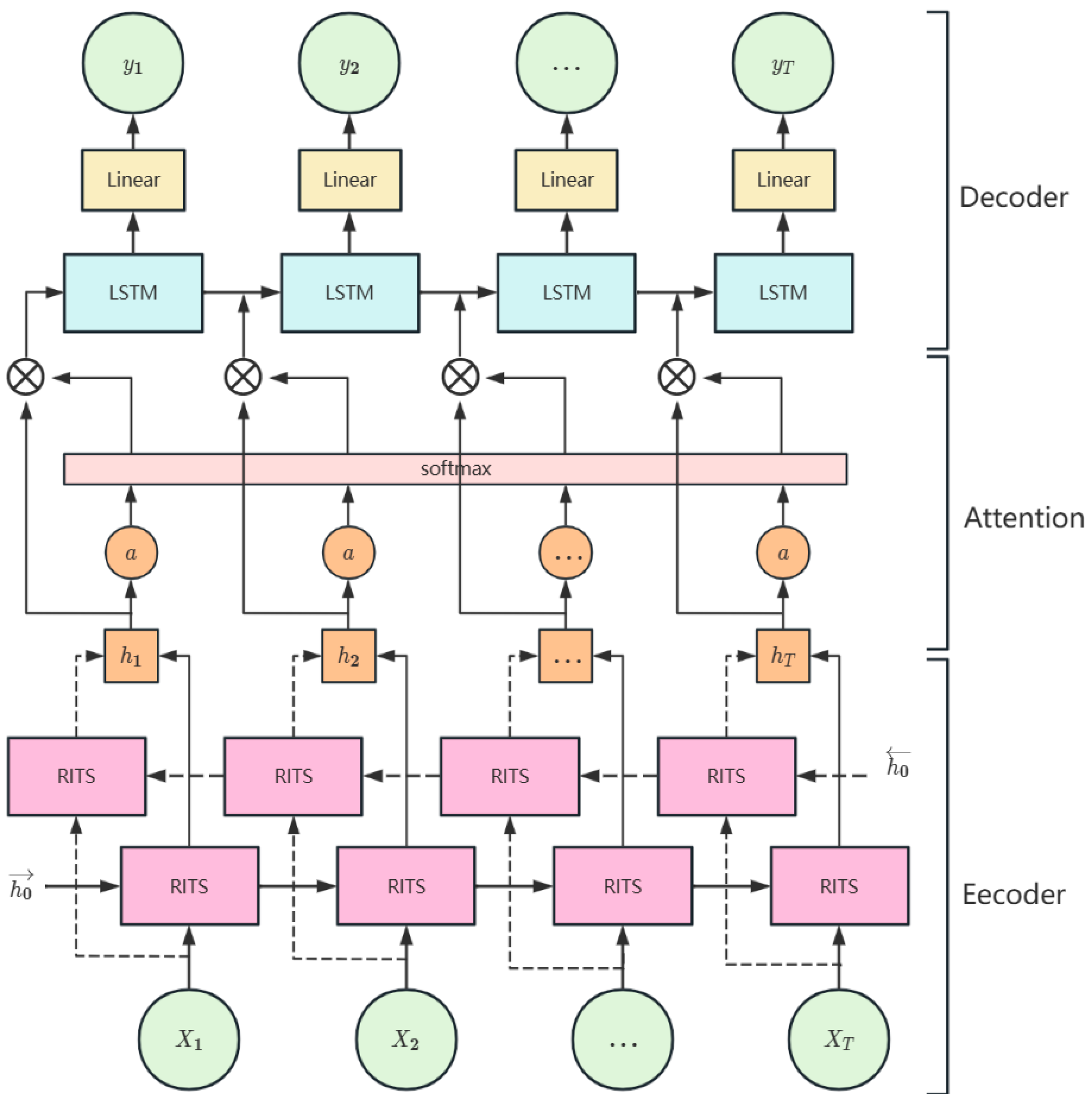
- The BRITS-ALSTM model employs a bidirectional encoding scheme complemented by a decoding architecture that incorporates an attention mechanism. This model is designed to capture both temporal dependencies and spatial correlations among adjacent stations at hourly intervals within a specified timeframe. Through the integration of the attention mechanism, it is possible to discern the significance of various informational inputs by assigning appropriate weight ratios, thereby fine-tuning the current state’s dependencies throughout the LSTM’s decoding phase.
- An analysis was conducted on the imputation of missing values in six categories of air quality data from 16 monitoring stations in Qinghai Province using three methods: mean-filling, BRITS (Bidirectional Recurrent Imputation for Time Series), and BRITS-ALSTM. The findings indicate that the BRITS-ALSTM model exhibits superior imputation accuracy, thereby enhancing the assessment of regional air quality data on the Tibetan Plateau.
2. Materials and Methods
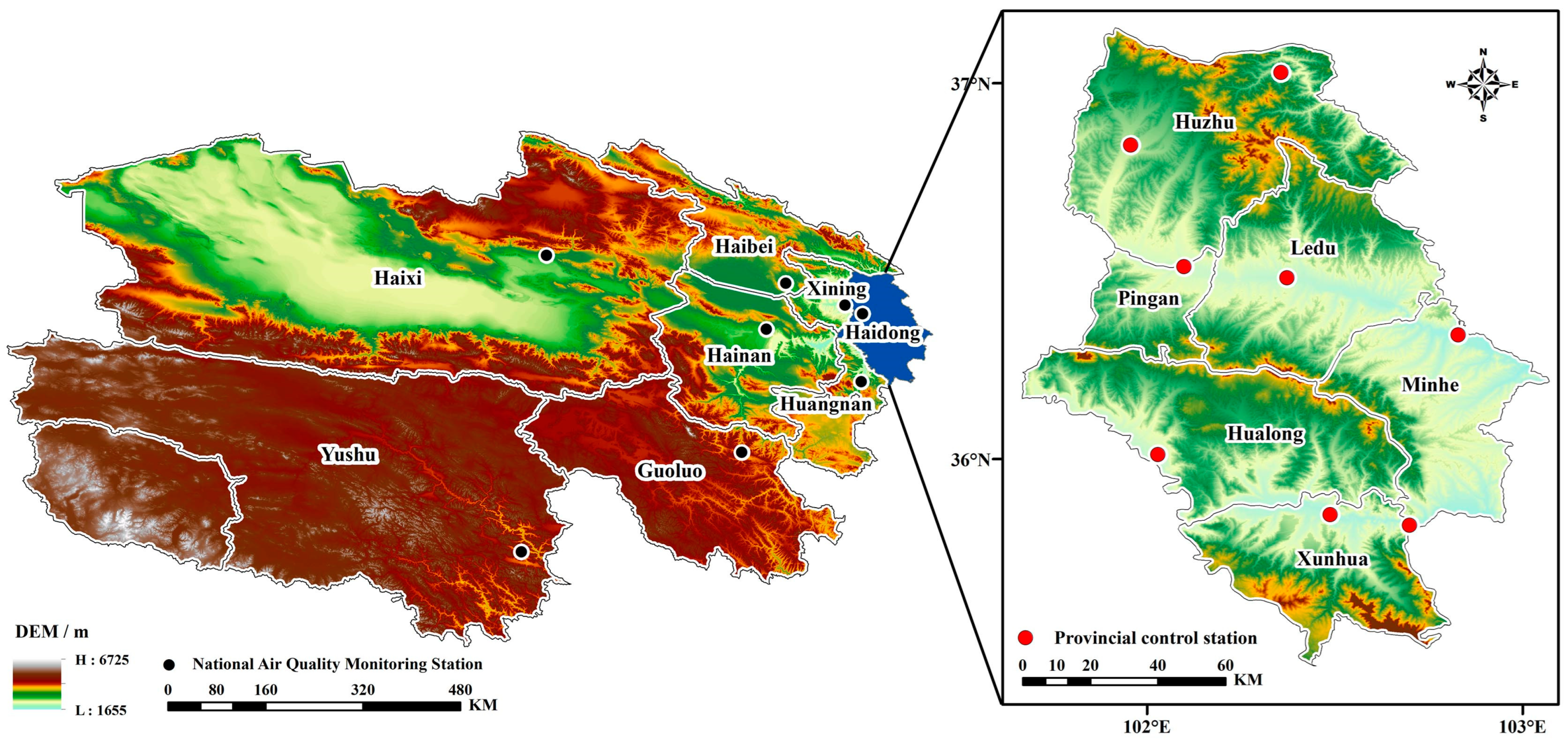
2.1. Data
2.2. Methodology
2.2.1. Basic Definition
2.2.2. BRITS-ALSTM Model
- Encoder
- 2.
- Attention Mechanism
- 3.
- Decoder
2.2.3. Evaluation Metrics
3. Results
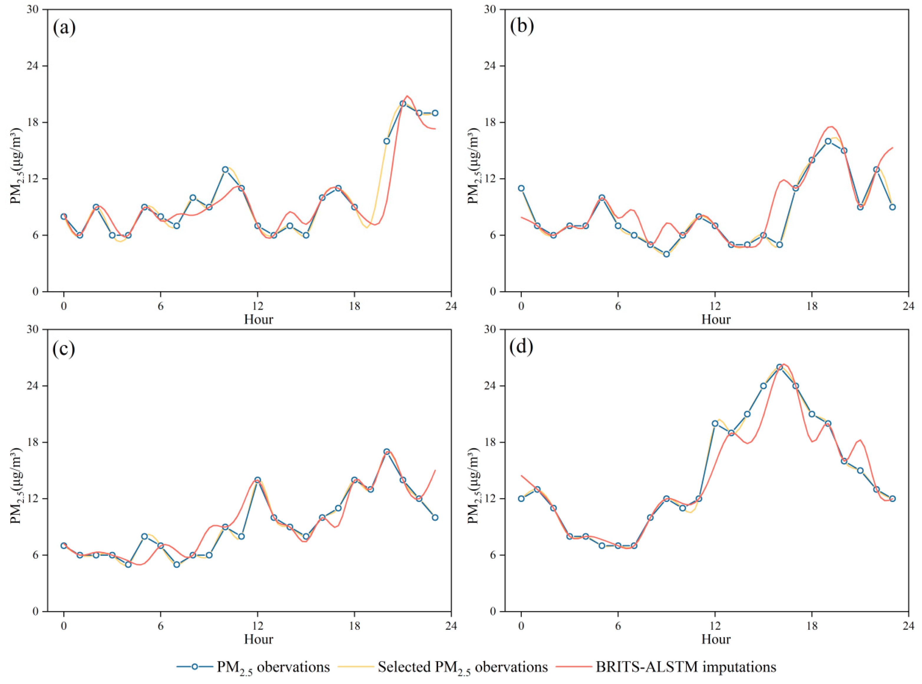
4. Discussion
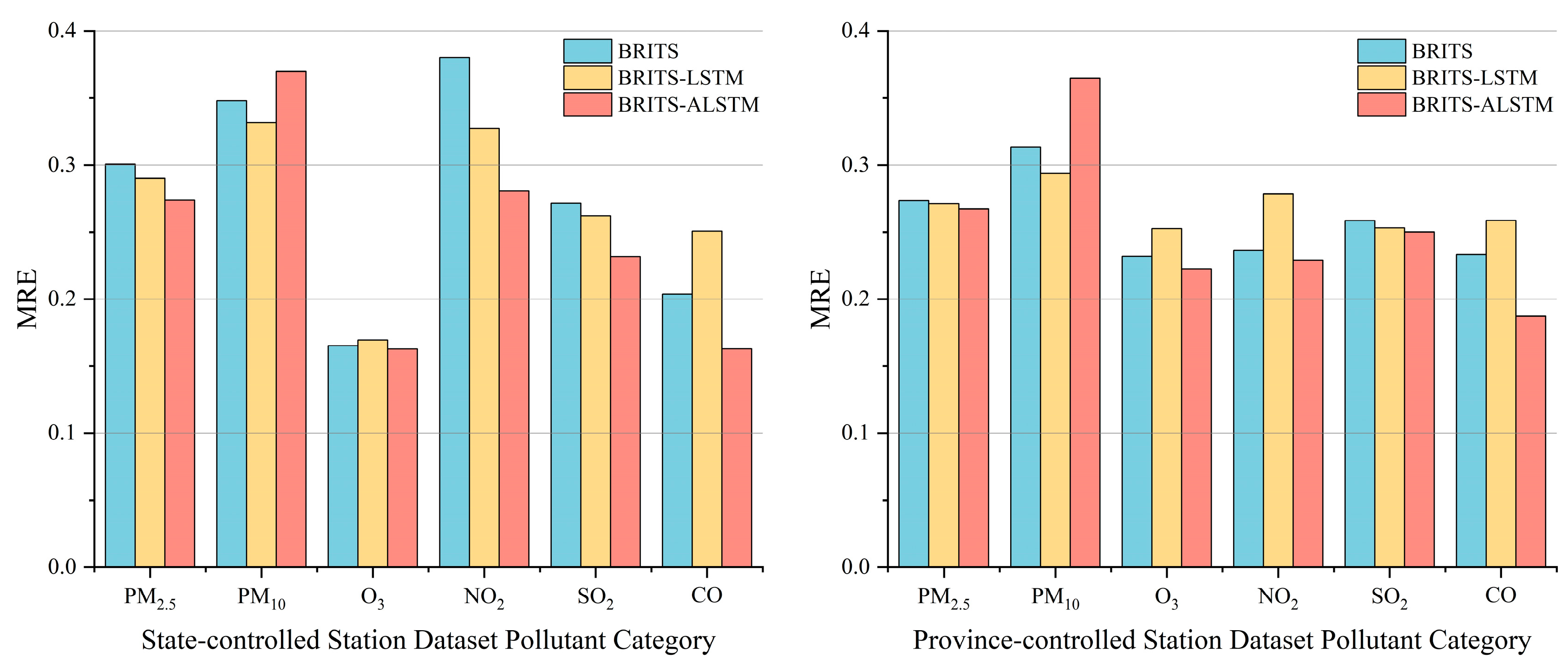
4.1. BRITS vs. BRITS-ALSTM
4.2. Application of BRITS-ALSTM Imputed Dataset
5. Conclusions
Author Contributions
Funding
Institutional Review Board Statement
Informed Consent Statement
Data Availability Statement
Conflicts of Interest
References
- Zhou, Y.; Luo, B.; Li, J.; Hao, Y.; Yang, W.; Shi, F.; Chen, Y.; Simayi, M.; Xie, S. Characteristics of six criteria air pollutants before, during, and after a severe air pollution episode caused by biomass burning in the southern Sichuan Basin, China. Atmos. Environ. 2019, 215, 116840. [Google Scholar] [CrossRef]
- Ebelt, S.T.; D’Souza, R.R.; Yu, H.; Scovronick, N.; Moss, S.; Chang, H.H. Monitoring vs. modeled exposure data in time-series studies of ambient air pollution and acute health outcomes. J. Expo. Sci. Environ. Epidemiol. 2023, 33, 377–385. [Google Scholar] [CrossRef] [PubMed]
- Fan, H.; Zhao, C.; Yang, Y. A comprehensive analysis of the spatio-temporal variation of urban air pollution in China during 2014–2018. Atmos. Environ. 2020, 220, 117066. [Google Scholar] [CrossRef]
- Lee, H.; Lee, J.; Oh, S.; Park, S.; Mayer, H. Air pollution assessment in Seoul, South Korea, using an updated daily air quality index. Atmos. Pollut. Res. 2023, 14, 101728. [Google Scholar] [CrossRef]
- Zou, B.; You, J.; Lin, Y.; Duan, X.; Zhao, X.; Fang, X.; Campen, M.J.; Li, S. Air pollution intervention and life-saving effect in China. Environ. Int. 2019, 125, 529–541. [Google Scholar] [CrossRef]
- Tzanis, C.G.; Alimissis, A.; Koutsogiannis, I. Addressing missing environmental data via a machine learning scheme. Atmosphere 2021, 12, 499. [Google Scholar] [CrossRef]
- Kadow, C.; Hall, D.M.; Ulbrich, U. Artificial intelligence reconstructs missing climate information. Nat. Geosci. 2020, 13, 408–413. [Google Scholar] [CrossRef]
- Singh, D.; Dahiya, M.; Kumar, R.; Nanda, C. Sensors and systems for air quality assessment monitoring and management: A review. J. Environ. Manag. 2021, 289, 112510. [Google Scholar] [CrossRef]
- Motlagh, N.H.; Lagerspetz, E.; Nurmi, P.; Li, X.; Varjonen, S.; Mineraud, J.; Siekkinen, M.; Rebeiro-Hargrave, A.; Hussein, T.; Petaja, T. Toward massive scale air quality monitoring. IEEE Commun. Mag. 2020, 58, 54–59. [Google Scholar] [CrossRef]
- Nasir, H.; Goyal, K.; Prabhakar, D. Review of air quality monitoring: Case study of India. Indian J. Sci. Technol. 2016, 9, 105255. [Google Scholar] [CrossRef]
- Feng, Y.; Ning, M.; Lei, Y.; Sun, Y.; Liu, W.; Wang, J. Defending blue sky in China: Effectiveness of the “Air Pollution Prevention and Control Action Plan” on air quality improvements from 2013 to 2017. J. Environ. Manag. 2019, 252, 109603. [Google Scholar] [CrossRef] [PubMed]
- Feenstra, B.; Papapostolou, V.; Hasheminassab, S.; Zhang, H.; Der Boghossian, B.; Cocker, D.; Polidori, A. Performance evaluation of twelve low-cost PM2.5 sensors at an ambient air monitoring site. Atmos. Environ. 2019, 216, 116946. [Google Scholar] [CrossRef]
- Zhao, A.; Nie, Y.; Hou, X.; Li, Y.; Li, H. Development of an unmanned 10-factor automatic weather station for cold and arid regions. Highl. Meteorol. 2003, 2003, 646–649. [Google Scholar]
- Wijesekara, L.; Liyanage, L. Mind the Large Gap: Novel Algorithm Using Seasonal Decomposition and Elastic Net Regression to Impute Large Intervals of Missing Data in Air Quality Data. Atmosphere 2023, 14, 355. [Google Scholar] [CrossRef]
- Liu, Y.; Zhou, Y.; Lu, J. Exploring the relationship between air pollution and meteorological conditions in China under environmental governance. Sci. Rep. 2020, 10, 14518. [Google Scholar] [CrossRef]
- Zhang, Y.; Thorburn, P.J. Handling missing data in near real-time environmental monitoring: A system and a review of selected methods. Future Gener. Comput. Syst. 2022, 128, 63–72. [Google Scholar] [CrossRef]
- Ottosen, T.-B.; Kumar, P. Outlier detection and gap filling methodologies for low-cost air quality measurements. Environ. Sci. Process. Impacts 2019, 21, 701–713. [Google Scholar] [CrossRef]
- Rashid, W.; Gupta, M.K. A perspective of missing value imputation approaches. In Proceedings of the Advances in Computational Intelligence and Communication Technology (CICT 2019), Allahabad, India, 6–8 December 2019; Springer: Berlin/Heidelberg, Germany, 2021; pp. 307–315. [Google Scholar]
- Armina, R.; Zain, A.M.; Ali, N.A.; Sallehuddin, R. A review on missing value estimation using imputation algorithm. J. Phys. Conf. Ser. 2017, 892, 012004. [Google Scholar] [CrossRef]
- Egigu, M. Techniques of Filling Missing Values of Daily and Monthly Rain Fall Data: A Review. SF J. Environ. Earth Sci. 2020, 3, 1036. [Google Scholar]
- Mao, Y.; Zhang, J.; Qi, H.; Wang, L. DNN-MVL: DNN-multi-view-learning-based recover block missing data in a dam safety monitoring system. Sensors 2019, 19, 2895. [Google Scholar] [CrossRef]
- Samal, K.K.R.; Babu, K.S.; Das, S.K. Multi-directional temporal convolutional artificial neural network for PM2.5 forecasting with missing values: A deep learning approach. Urban Clim. 2021, 36, 100800. [Google Scholar] [CrossRef]
- Marchang, N.; Tripathi, R. KNN-ST: Exploiting spatio-temporal correlation for missing data inference in environmental crowd sensing. IEEE Sens. J. 2020, 21, 3429–3436. [Google Scholar] [CrossRef]
- Ma, J.; Cheng, J.C.; Ding, Y.; Lin, C.; Jiang, F.; Wang, M.; Zhai, C. Transfer learning for long-interval consecutive missing values imputation without external features in air pollution time series. Adv. Eng. Inform. 2020, 44, 101092. [Google Scholar] [CrossRef]
- Tang, J.; Zhang, X.; Yin, W.; Zou, Y.; Wang, Y. Missing data imputation for traffic flow based on combination of fuzzy neural network and rough set theory. J. Intell. Transp. Syst. 2021, 25, 439–454. [Google Scholar] [CrossRef]
- Baloch, M.A.; Wang, B. Analyzing the role of governance in CO2 emissions mitigation: The BRICS experience. Struct. Chang. Econ. Dyn. 2019, 51, 119–125. [Google Scholar]
- Worden, K.; Sohn, H.; Farrar, C.R. Novelty detection in a changing environment: Regression and interpolation approaches. J. Sound Vib. 2002, 258, 741–761. [Google Scholar] [CrossRef]
- Noor, M.; Yahaya, A.; Ramli, N.A.; Al Bakri, A.M. Filling missing data using interpolation methods: Study on the effect of fitting distribution. Key Eng. Mater. 2014, 594, 889–895. [Google Scholar] [CrossRef]
- Junninen, H.; Niska, H.; Tuppurainen, K.; Ruuskanen, J.; Kolehmainen, M. Methods for imputation of missing values in air quality data sets. Atmos. Environ. 2004, 38, 2895–2907. [Google Scholar] [CrossRef]
- Norazian, M.; Al Bakri, A.M.M.; Shukri, Y.A.; Azam, R.N. Estimation of missing values for air pollution data using interpolation technique. Simulation 2006, 75, 94. [Google Scholar]
- Saeipourdizaj, P.; Sarbakhsh, P.; Gholampour, A. Application of imputation methods for missing values of PM10 and O3 data: Interpolation, moving average and K-nearest neighbor methods. Environ. Health Eng. Manag. J. 2021, 8, 215–226. [Google Scholar] [CrossRef]
- Honghai, F.; Guoshun, C.; Cheng, Y.; Bingru, Y.; Yumei, C. A SVM regression based approach to filling in missing values. In Proceedings of the International Conference on Knowledge-Based and Intelligent Information and Engineering Systems, Melbourne, Australia, 14–16 September 2005; pp. 581–587. [Google Scholar]
- Patil, B.M.; Joshi, R.C.; Toshniwal, D. Missing value imputation based on k-mean clustering with weighted distance. In Proceedings of the Contemporary Computing: Third International Conference (IC3 2010), Noida, India, 9–11 August 2010; Proceedings Part I3. Springer: Berlin/Heidelberg, Germany, 2010; pp. 600–609. [Google Scholar]
- Kornelsen, K.; Coulibaly, P. Comparison of interpolation, statistical, and data-driven methods for imputation of missing values in a distributed soil moisture dataset. J. Hydrol. Eng. 2014, 19, 26–43. [Google Scholar] [CrossRef]
- Ye, Z.; Yang, J.; Zhong, N.; Tu, X.; Jia, J.; Wang, J. Tackling environmental challenges in pollution controls using artificial intelligence: A review. Sci. Total Environ. 2020, 699, 134279. [Google Scholar] [CrossRef] [PubMed]
- Che, Z.; Purushotham, S.; Cho, K.; Sontag, D.; Liu, Y. Recurrent neural networks for multivariate time series with missing values. Sci. Rep. 2018, 8, 6085. [Google Scholar] [CrossRef]
- Cao, W.; Wang, D.; Li, J.; Zhou, H.; Li, L.; Li, Y. Brits: Bidirectional recurrent imputation for time series. In Proceedings of the Annual Conference on Neural Information Processing Systems 2018, NeurIPS 2018, Montréal, Canada, 3–8 December 2018; Volume 31. [Google Scholar]
- Yoon, J.; Jordon, J.; Schaar, M. Gain: Missing data imputation using generative adversarial nets. In Proceedings of the 35th International Conference on Machine Learning, Stockholm, Sweden, 10–15 July 2018; pp. 5689–5698. [Google Scholar]
- Cini, A.; Marisca, I.; Alippi, C. Filling the g_ap_s: Multivariate time series imputation by graph neural networks. arXiv 2021, arXiv:2108.00298. [Google Scholar]
- Ma, J.; Cheng, J.C.; Jiang, F.; Chen, W.; Wang, M.; Zhai, C. A bi-directional missing data imputation scheme based on LSTM and transfer learning for building energy data. Energy Build. 2020, 216, 109941. [Google Scholar] [CrossRef]
- Yin, Y.; Shi, C.; Zou, C.; Liu, X. Fusion of Seq2Seq and temporal attention mechanism for process quality prediction. Mech. Sci. Technol. 2019, 107, 287–300. [Google Scholar] [CrossRef]
- Weerakody, P.B.; Wong, K.W.; Wang, G.; Ela, W. A review of irregular time series data handling with gated recurrent neural networks. Neurocomputing 2021, 441, 161–178. [Google Scholar] [CrossRef]
- Iskandaryan, D.; Ramos, F.; Trilles, S. Air quality prediction in smart cities using machine learning technologies based on sensor data: A review. Appl. Sci. 2020, 10, 2401. [Google Scholar] [CrossRef]
- Chen, H.; Guan, M.; Li, H. Air quality prediction based on integrated dual LSTM model. IEEE Access 2021, 9, 93285–93297. [Google Scholar] [CrossRef]
- Liu, B.; Yan, S.; Li, J.; Qu, G.; Li, Y.; Lang, J.; Gu, R. A sequence-to-sequence air quality predictor based on the n-step recurrent prediction. IEEE Access 2019, 7, 43331–43345. [Google Scholar] [CrossRef]
- Zhu, Z.; Rao, Y.; Wu, Y.; Qi, H.; Zhang, Y. Research Progress of Attentional Mechanisms in Deep Learning. J. Chin. Inf. 2019, 33, 1–11. [Google Scholar]
- Utama, I.B.K.Y.; Tran, D.H.; Jang, Y.M. Short-term PM2.5 Prediction using Modified Attention Seq2Seq BiLSTM. In Proceedings of the 2022 Thirteenth International Conference on Ubiquitous and Future Networks (ICUFN), Barcelona, Spain, 5–8 July 2022; pp. 462–465. [Google Scholar]
- Tu, X.-Y.; Zhang, B.; Jin, Y.-P.; Zou, G.-J.; Pan, J.-G.; Li, M.-Z. Longer time span air pollution prediction: The attention and autoencoder hybrid learning model. Math. Probl. Eng. 2021, 2021, 5515103. [Google Scholar] [CrossRef]
- Caiji, Z. Construction and empirical research on differentiated evaluation index system for ecological civilization construction in Qinghai Province. Ecol. Econ. 2023, 39, 214–220. [Google Scholar]
- Sun, H.; Zheng, D.; Yao, T.; Zhang, Y. Protection and construction of national ecological security barriers on the Tibetan Plateau. J. Geogr. 2012, 67, 3–12. [Google Scholar]
- Liang, G. Practical exploration of intelligent operation and maintenance platform construction for ambient air automatic stations. Sci. Technol. Innov. 2020, 2020, 138–139. [Google Scholar] [CrossRef]
- Xie, C.; Huang, C.; Zhang, D.; He, W. BiLSTM-I: A deep learning-based long interval gap-filling method for meteorological observation data. Int. J. Environ. Res. Public Health 2021, 18, 10321. [Google Scholar] [CrossRef]
- Shuai, P.; Li, X.; Zhou, X.; Liu, Y. Research Progress on Statistical Processing Methods for Missing Data. China Health Stat. 2013, 30, 135–139+142. [Google Scholar]
- Hwang, W.-S.; Li, S.; Kim, S.-W.; Lee, K. Data imputation using a trust network for recommendation via matrix factorization. Comput. Sci. Inf. Syst. 2018, 15, 347–368. [Google Scholar] [CrossRef]
- Van Buuren, S.; Groothuis-Oudshoorn, K. mice: Multivariate imputation by chained equations in R. J. Stat. Softw. 2011, 45, 1–67. [Google Scholar] [CrossRef]
- Yoon, J.; Zame, W.R.; van der Schaar, M. Multi-directional recurrent neural networks: A novel method for estimating missing data. In Proceedings of the Time Series Workshop in International Conference on Machine Learning, New Orleans, LA, USA, 18–21 November 2017. [Google Scholar]
- Xing, Y.; Brimblecombe, P. Role of vegetation in deposition and dispersion of air pollution in urban parks. Atmos. Environ. 2019, 201, 73–83. [Google Scholar] [CrossRef]


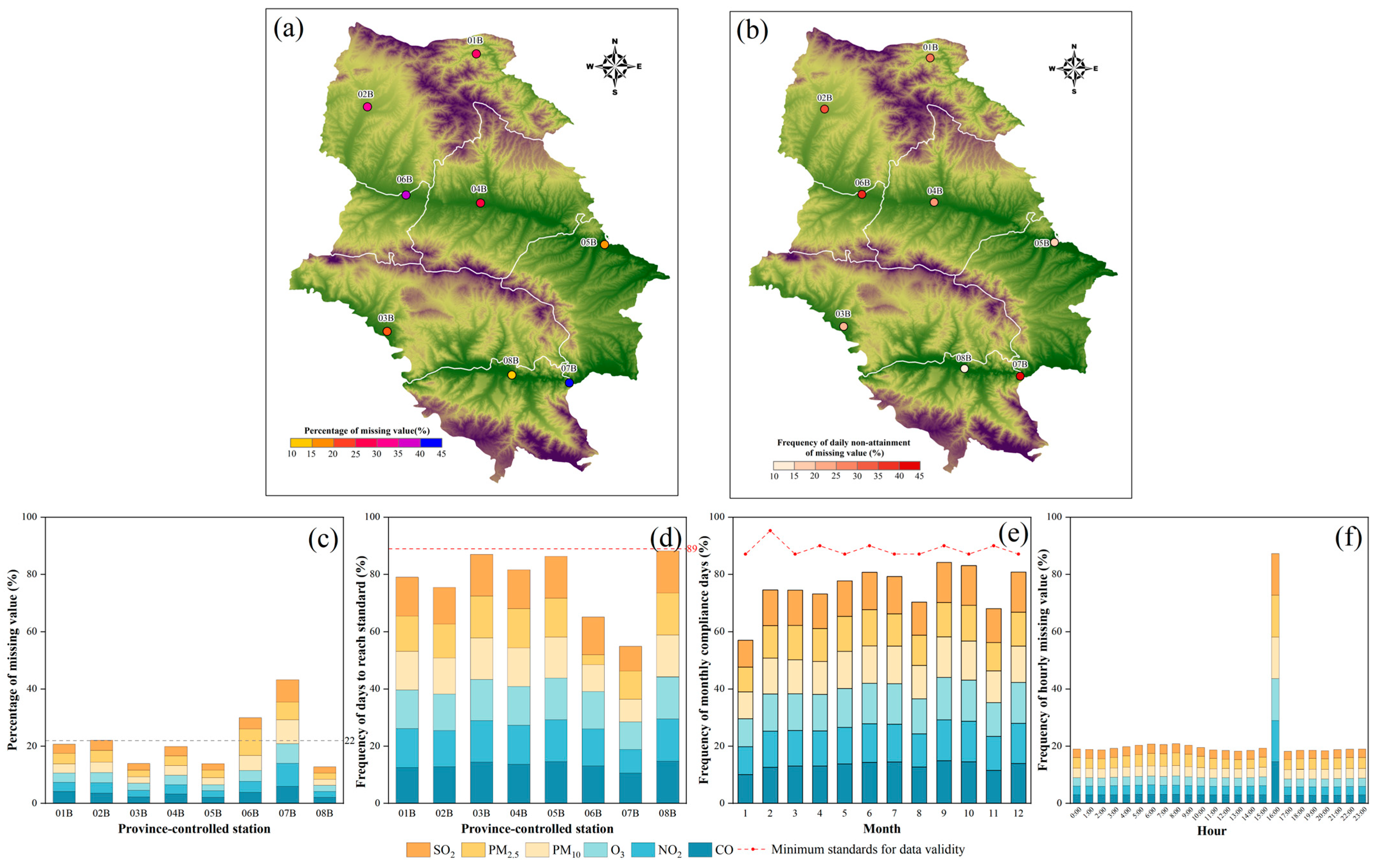
| Pollutant | Average Time | Data Validity Requirement |
|---|---|---|
| PM2.5, PM10, NO2, SO2 | annual average | Condition 1: At least 324 daily average concentration values yearly. Condition 2: At least 27 daily average concentration values monthly (with February necessitating at least 25 values). |
| PM2.5, PM10, NO2, SO2, and CO | 24-h average | At least 20 h of average concentration values or sampling time daily. |
| O3 | 8-h average | At least 6 hourly averaged concentration values for every 8 h. |
| S1 | S2 | S3 | S4 | S5 | S6 | S7 | S8 | m1 | m2 | m3 | m4 | m5 | m6 | m7 | m8 | δ1 | δ2 | δ3 | δ4 | δ5 | δ6 | δ7 | δ8 | |
|---|---|---|---|---|---|---|---|---|---|---|---|---|---|---|---|---|---|---|---|---|---|---|---|---|
| 1 January 2019 0:00 | - | 37 | 28 | - | - | 8 | 54 | 98 | 0 | 1 | 1 | 0 | 0 | 1 | 1 | 1 | 1 | 1 | 1 | 1 | 1 | 1 | 1 | 1 |
| 1 January 2019 1:00 | 9 | 40 | 25 | - | - | 6 | 66 | 97 | 1 | 1 | 1 | 0 | 0 | 1 | 1 | 1 | 1 | 1 | 1 | 2 | 2 | 1 | 1 | 1 |
| 1 January 2019 2:00 | 7 | 40 | 25 | - | - | 9 | 68 | 90 | 1 | 1 | 1 | 0 | 0 | 1 | 1 | 1 | 1 | 1 | 1 | 3 | 3 | 1 | 1 | 1 |
| 1 January 2019 3:00 | 16 | 44 | 19 | - | - | 6 | 75 | 94 | 1 | 1 | 1 | 0 | 0 | 1 | 1 | 1 | 1 | 1 | 1 | 4 | 4 | 1 | 1 | 1 |
| 1 January 2019 4:00 | 25 | 46 | 18 | - | - | 6 | 77 | 94 | 1 | 1 | 1 | 0 | 0 | 1 | 1 | 1 | 1 | 1 | 1 | 5 | 5 | 1 | 1 | 1 |
| 1 January 2019 5:00 | 23 | 41 | 20 | - | - | 9 | 75 | 85 | 1 | 1 | 1 | 0 | 0 | 1 | 1 | 1 | 1 | 1 | 1 | 6 | 6 | 1 | 1 | 1 |
| 1 January 2019 6:00 | 20 | 34 | 16 | - | 15 | 8 | 74 | 87 | 1 | 1 | 1 | 0 | 1 | 1 | 1 | 1 | 1 | 1 | 1 | 7 | 1 | 1 | 1 | 1 |
| 1 January 2019 7:00 | 21 | 29 | 17 | - | 12 | 7 | 83 | 96 | 1 | 1 | 1 | 0 | 1 | 1 | 1 | 1 | 1 | 1 | 1 | 8 | 1 | 1 | 1 | 1 |
| Method | Introduction |
|---|---|
| Mean | Use a simple global average to replace missing values [53]. |
| KNN | K-nearest neighbor imputes the missing values by finding similar samples and using the weighted average of their neighbors [53]. |
| MF | The Matrix Factorization method decomposes the data matrix into two low-rank matrices and fills in the missing values by means of matrix completion [54]. |
| MICE | Create multiple imputations using chained equations [55]. |
| M-RNN | Missing values are imputed based on the hidden states in both directions in a bidirectional RNN [56]. |
| State-Controlled Station Dataset (Missing Rate) | PM2.5 (5.70%) | PM10 (5.70%) | O3 (4.96%) | NO2 (4.86%) | SO2 (4.77%) | CO (5.00%) | ||||||
|---|---|---|---|---|---|---|---|---|---|---|---|---|
| Method | MAE | MRE | MAE | MRE | MAE | MRE | MAE | MRE | MAE | MRE | MAE | MRE |
| Mean | 21.4726 | 0.9944 | 47.5001 | 1.0070 | 74.8322 | 0.9994 | 17.7608 | 0.9966 | 13.1555 | 0.9867 | 0.6231 | 0.9961 |
| KNN | 21.2697 | 0.9881 | 46.9564 | 0.9954 | 75.9053 | 1.0137 | 17.2510 | 0.9680 | 12.9697 | 0.9728 | 0.6187 | 0.9893 |
| MF | 18.5589 | 0.9592 | 28.2112 | 0.5612 | 70.3940 | 0.8156 | 19.9263 | 1.0599 | 9.4305 | 0.8431 | 0.8335 | 0.9737 |
| MICE | 22.5469 | 1.0132 | 48.2395 | 1.0171 | 73.2109 | 1.0014 | 19.3482 | 1.0064 | 13.5124 | 1.0135 | 0.6546 | 1.0087 |
| M-RNN | 6.7744 | 0.3115 | 20.7425 | 0.4352 | 18.7845 | 0.2483 | 5.7384 | 0.3187 | 3.7013 | 0.2772 | 0.1403 | 0.2220 |
| BRITS | 6.4716 | 0.3007 | 16.0573 | 0.3478 | 12.5022 | 0.1653 | 6.0460 | 0.3802 | 3.6611 | 0.2717 | 0.1288 | 0.2038 |
| BRITS-LATM | 6.3088 | 0.2901 | 15.8079 | 0.3317 | 12.8271 | 0.1696 | 5.8899 | 0.3272 | 3.5000 | 0.2621 | 0.1584 | 0.2507 |
| BRITS-ALSTM | 5.9780 | 0.2739 | 17.6502 | 0.3698 | 12.4189 | 0.1629 | 5.0359 | 0.2805 | 3.0694 | 0.2317 | 0.1030 | 0.1630 |
| Province-Controlled Station Dataset (Missing Rate) | PM2.5 (25.35%) | PM10 (23.03%) | O3 (20.67%) | NO2 (21.48%) | SO2 (21.26%) | CO (20.64%) | ||||||
|---|---|---|---|---|---|---|---|---|---|---|---|---|
| Method | MAE | MRE | MAE | MRE | MAE | MRE | MAE | MRE | MAE | MRE | MAE | MRE |
| Mean | 27.8987 | 0.9913 | 54.3233 | 0.9919 | 73.1636 | 0.9984 | 16.0976 | 0.9956 | 11.7414 | 0.9996 | 0.4681 | 0.9978 |
| KNN | 27.8212 | 0.9885 | 54.0408 | 0.9868 | 73.7039 | 1.0058 | 15.6014 | 0.9649 | 11.7324 | 0.9988 | 0.4625 | 0.9859 |
| MF | 21.9874 | 0.9875 | 27.5499 | 0.5180 | 68.3819 | 1.0563 | 13.7795 | 0.6732 | 10.0977 | 0.9857 | 0.4592 | 1.0061 |
| MICE | 28.2986 | 1.0055 | 57.9825 | 1.0094 | 73.4007 | 1.0017 | 15.7524 | 1.0071 | 12.4394 | 1.0206 | 0.4732 | 1.008 |
| M-RNN | 10.3735 | 0.3402 | 24.7701 | 0.4183 | 29.6608 | 0.3754 | 5.1823 | 0.2971 | 3.7853 | 0.2987 | 0.1312 | 0.2593 |
| BRITS | 8.3332 | 0.2735 | 18.5450 | 0.3132 | 18.9782 | 0.2319 | 4.1258 | 0.2365 | 3.2621 | 0.2586 | 0.1179 | 0.2331 |
| BRITS-LATM | 8.2768 | 0.2714 | 17.4104 | 0.2940 | 19.9559 | 0.2526 | 4.8560 | 0.2784 | 3.2093 | 0.2532 | 0.1301 | 0.2587 |
| BRITS-ALSTM | 8.1505 | 0.2672 | 22.7985 | 0.3648 | 17.5627 | 0.2223 | 3.9949 | 0.2290 | 3.1693 | 0.2501 | 0.0947 | 0.1872 |
| Method | State-Controlled Station Dataset (5%) | Province-Controlled Station Dataset (22%) | ||||
|---|---|---|---|---|---|---|
| Mean | 0.9967 | 0% | −0.8763 | 0.9958 | 0% | 0.1676 |
| BRITS | 0.2783 | 72.08% | −6.3038 | 0.2578 | 74.11% | −1.1276 |
| BRITS-LSTM | 0.2719 | 72.72% | −5.9729 | 0.2681 | 73.08% | −0.4603 |
| BRITS-ALSTM | 0.2470 | 75.22% | −12.0141 | 0.2534 | 74.54% | −1.8424 |
| Pollutant | State-Controlled Station Dataset | Province-Controlled Station Dataset | ||||||
|---|---|---|---|---|---|---|---|---|
| RMSE | R2 | RMSE | R2 | |||||
| Mean | BRITS-ALSTM | Mean | BRITS-ALSTM | Mean | BRITS-ALSTM | Mean | BRITS-ALSTM | |
| PM2.5 | 6.7655 | 6.7641 | 0.7579 | 0.7586 | 6.1995 | 5.9208 | 0.5708 | 0.5894 |
| PM10 | 22.6113 | 22.6090 | 0.7898 | 0.7919 | 15.2148 | 15.0954 | 0.6610 | 0.6721 |
| O3 | 10.0555 | 9.8906 | 0.8782 | 0.8852 | 83.3033 | 66.8887 | 0.8100 | 0.8856 |
| NO2 | 4.2449 | 4.2350 | 0.7016 | 0.7073 | 1.3809 | 1.2662 | 0.9318 | 0.9450 |
| SO2 | 18.7112 | 18.2332 | 0.4370 | 0.4671 | 5.8258 | 5.3867 | 0.8078 | 0.8428 |
| CO | 0.0916 | 0.0890 | 0.8257 | 0.8314 | 0.03608 | 0.0353 | 0.9454 | 0.9604 |
Disclaimer/Publisher’s Note: The statements, opinions and data contained in all publications are solely those of the individual author(s) and contributor(s) and not of MDPI and/or the editor(s). MDPI and/or the editor(s) disclaim responsibility for any injury to people or property resulting from any ideas, methods, instructions or products referred to in the content. |
© 2023 by the authors. Licensee MDPI, Basel, Switzerland. This article is an open access article distributed under the terms and conditions of the Creative Commons Attribution (CC BY) license (https://creativecommons.org/licenses/by/4.0/).
Share and Cite
Wang, Y.; Liu, K.; He, Y.; Fu, Q.; Luo, W.; Li, W.; Liu, X.; Wang, P.; Xiao, S. Research on Missing Value Imputation to Improve the Validity of Air Quality Data Evaluation on the Qinghai-Tibetan Plateau. Atmosphere 2023, 14, 1821. https://doi.org/10.3390/atmos14121821
Wang Y, Liu K, He Y, Fu Q, Luo W, Li W, Liu X, Wang P, Xiao S. Research on Missing Value Imputation to Improve the Validity of Air Quality Data Evaluation on the Qinghai-Tibetan Plateau. Atmosphere. 2023; 14(12):1821. https://doi.org/10.3390/atmos14121821
Chicago/Turabian StyleWang, Yumeng, Ke Liu, Yuejun He, Qiming Fu, Wei Luo, Wentao Li, Xuan Liu, Pengfei Wang, and Siyuan Xiao. 2023. "Research on Missing Value Imputation to Improve the Validity of Air Quality Data Evaluation on the Qinghai-Tibetan Plateau" Atmosphere 14, no. 12: 1821. https://doi.org/10.3390/atmos14121821
APA StyleWang, Y., Liu, K., He, Y., Fu, Q., Luo, W., Li, W., Liu, X., Wang, P., & Xiao, S. (2023). Research on Missing Value Imputation to Improve the Validity of Air Quality Data Evaluation on the Qinghai-Tibetan Plateau. Atmosphere, 14(12), 1821. https://doi.org/10.3390/atmos14121821