Article

A Methodological Approach for Gap Filling of WFV Gaofen-1 Images from Spatial Autocorrelation and Enhanced Weighting

1
Aerospace Information Research Institute, Chinese Academy of Sciences, Beijing 100094, China
2
School of Remote Sensing and Information Engineering, North China Institute of Aerospace Engineering, Langfang 065000, China
*
Author to whom correspondence should be addressed.
Atmosphere 2024, 15(3), 252; https://doi.org/10.3390/atmos15030252
Submission received: 24 January 2024 / Revised: 16 February 2024 / Accepted: 19 February 2024 / Published: 21 February 2024
(This article belongs to the Special Issue Atmospheric Environment and Agro-Ecological Environment)

Abstract

:
Clouds and cloud shadow cover cause missing data in some images captured by the Gaofen-1 Wide Field of View (GF-1 WFV) cameras, limiting the extraction and analysis of the image information and further applications. Therefore, this study proposes a methodology to fill GF-1 WFV images using the spatial autocorrelation and improved weighting (SAIW) method. Specifically, the search window size is adaptively determined using Getis-Ord Gi* as a metric. The spatial and spectral weights of the pixels are computed using the Chebyshev distance and spectral angle mapper to better filter the suitable similar pixels. Each missing pixel is predicted using linear regression with similar pixels on the reference image and the corresponding similar pixel located in the non-missing region of the cloudy image. Simulation experiments showed that the average correlation coefficient of the proposed method in this study is 0.966 in heterogeneous areas, 0.983 in homogeneous farmland, and 0.948 in complex urban areas. It suggests that SAIW can reduce the spread of errors in the gap-filling process to significantly improve the accuracy of the filling results and can produce satisfactory qualitative and quantitative fill results in a wide range of typical land cover types and has extensive application potential.

1. Introduction

With the rapid development of remote sensing sensors and platforms, high-resolution remote sensing images are becoming more readily available [1]. The copious and more detailed information provided in high-resolution remote sensing images has led to a wide range of applications in the areas of monitoring natural disasters (e.g., floods [2], forest fires [3], and earthquakes [4]) and human activities (e.g., land use/land cover classification [5], change detection [6]). The Gaofen-1 satellite is the first satellite of the China High-resolution Earth Observation System (CHEOS) and has been continuously acquiring massive amounts of Earth observation data since its operation in orbit in April 2013 [7]. The Wide Field of View (WFV) imaging system of the GF-1 satellite includes four wide-width cameras with a 16-m spatial resolution and a four-day revisit cycle. The swath width of the GF-1 WFV can reach up to 800 km when the four wide-width cameras are combined [8]. Currently, the image of the GF-1 satellite has been widely used in the fields of forestry [9,10], agriculture [11,12,13], and ecological environment [14,15], making up to a certain extent for the shortcomings in the application of high-resolution satellite data in China.
However, optical remote sensing images are often contaminated or covered by clouds and cloud shadows due to weather conditions, especially in summer, making real ground information missing and extremely limiting the application of optical images [16]. For this reason, many researchers have developed gap-filling methods for reconstructing missing data from cloud-covered images, which can be categorized into two main groups based on the source of the auxiliary information data used [17]: spatial-, temporal-, and spatiotemporal-based methods.
Spatial-based methods reconstruct the missing pixels of images using information from the remaining valid pixels in cloudy images without using other reference images. The most common are interpolation-based methods, such as Kriging interpolation [18,19]. Some researchers have also viewed reconstructing missing data as a pathological inverse problem and used regularization methods to solve these inverse problems [20,21,22]. Spatial-based methods may perform well for a few missing pixels or simple textures; however, they are unsatisfactory in coping with large cloud cover and complex heterogeneous regions.
Temporal-based methods provide reference information for reconstructing cloud-covered areas in target images based on data acquired at different times in the same study area. Temporal-based methods are usually more reliable than those of spatial-based methods, particularly for large-area gap filling; temporal-based cloud removal methods have been studied more thoroughly [23,24]. Pixels missing in the area of interest can typically be compensated for through temporal interpolation by multiple years’ average [25]. To enhance the reliability of predictions pertaining to pixel value changes within the covered area, the average values can be physically constrained by combining a priori knowledge, such as albedo phenology [26]. Temporal filter techniques are commonly used to smooth the time series for noise reduction purposes, making the albedo change consistent with the phenology trend [27]. Popular temporal filters include the Savitzky–Golay (SG) filter [28] and the mean-value iterative filter [29]. Additionally, noise reduction using curve fitting [30,31] and frequency domain transform [32] techniques are likewise common for time series reconstruction.
Spatiotemporal-based methods use complementary information in satellite images captured at adjacent times [33] to model the relationship between neighboring similar pixels of a cloudy image and other auxiliary data based on local correlation [34] to reduce or minimize discrepancies. Zhu et al. [35] proposed a modified neighborhood similar pixel interpolator (mNSPI) method that can fill in missing regions covered by clouds by combining local area replacement and interpolation. Zeng et al. [36] proposed a weighted linear regression (WLR) method for reconstructing missing data that uses multitemporal images as referable information and then constructs a regression model between the corresponding missing pixels. Similarly, spatiotemporal-based methods include spatially and temporally weighted regression (STWR) [37], spectral-angle-mapper-based spatial–temporal similarity (SAMSTS) [38], combined with Kalman filtering and surface energy balance theory [39], etc. In addition, more and more gap-filling methods using deep learning have been proposed in recent years. Examples include convolutional neural networks (CNN) [40], generative adversarial networks (GAN) [41,42], and recurrent neural networks (RNN) [43]. Deep learning methods use a moderate amount of multi-temporal data to achieve satisfactory accuracy. However, unlike some non-learning gap-filling methods that use only single-phase temporal reference information, deep learning methods usually require multi-phase temporal reference information to ensure sufficient image data to facilitate model training. The number of reference images that deep learning methods need to prepare increases exponentially as the area of interest increases. This may limit its large-scale application due to the reliance on large datasets, as well as the complexity and high computational performance requirements of the method.
When reconstructing missing pixels, searching for similar pixels to fill in missing regions usually involves using spectral or spatial information of the local spatial neighborhood or local temporal neighborhood images. The selection of the most correlated and suitable pixels similar to the target pixels determines the accuracy of the filling result. The search window determines the extent of the search for similar pixels in a localized region. If the window size is too small or too large, it could result in an inadequate amount of correlated pixels involved in the fill calculation, or alternatively, it might lead to the inclusion of more low-correlated pixels in the computation [44]. In the proposed research methods, the window size is usually set to a fixed value [45,46], or an error evaluation index is used to calculate the difference between the pixel values within the window to dynamically confirm the window size [47,48,49]. It only determines the window size from the perspective of spectral correlation and does not consider spatial autocorrelation. The search for similar pixels is accomplished using a correlation metric usually determined by weight calculations [37,38,50,51]. Commonly used spatial and spectral weights are calculated only from the perspective of two pixels, without much consideration of the structural distribution of nearby features, to assist in the search for similar pixels.
Most of the gap-filling methods that have been proposed are designed for low- and medium-resolution images, such as Landsat [50,52,53] and moderate-resolution imaging spectroradiometers (MODIS) [34,54,55]. Some studies have used medium- and high-resolution images from different satellites as auxiliary data [45,56]. Among the known gap-filling studies, there are only a few methodological studies on Gaofen-1 (GF-1) WFV gap filling.
Based on the above problems, in this study, we propose a GF-1 WFV image gap-filling method using spatial autocorrelation and improved weighting (SAIW). The novelty of this research stems from the following: (1) we propose a strategy to adaptively determine the search window size based on the local spatial autocorrelation; (2) in order to further clarify the spatial and spectral correlations between pixels, taking into account the feature distribution around pixels, Chebyshev distance and spectral angle mapping are used to improve spatial and spectral weights, respectively.

2. Materials and Methods

The main steps of the proposed method include the following: (1) data preprocessing, i.e., the panchromatic fusion of Landsat 8 OLI and resampling to 16 m spatial resolution; (2) adaptive selection of a suitable search window size; (3) selection of similar pixels, i.e., selection of pixels belonging to the same feature according to the unsupervised classification results; (4) screening of similar pixels, screening of a certain number of similar pixels based on spatial and spectral weights; and (5) prediction of the value of the missing pixels based on the linear regression model, and the specific process is shown in Figure 1.

2.1. Data

In this study, we used GF-1 WFV and Landsat 8 OLI images to validate the proposed method (Table 1). The Landsat OLI contains seven bands, whereas GF-1 contains only four bands (blue, green, red, and near-infrared (NIR) bands). Therefore, in our experiments, we only considered four bands (blue, green, red, and NIR bands).
Downscaling of the Landsat 8 OLI was required before filling, considering that the spatial resolutions of the GF-1 WFV and Landsat 8 OLI were 16 and 30 m, respectively. Panchromatic and multispectral image fusion [57] was applied to the Landsat 8 OLI images, resulting in an image with a resolution of 15 m. The fused image was resampled using bilinear interpolation to the same spatial resolution of 16 m as that of the GF-1 WFV.

2.2. Adaptive Search Window

Objects of land surface exhibit spatial aggregation in remote sensing images. Similar feature types tend to be spatially close or clustered with each other; this is defined as spatial autocorrelation [58]. This implies that a pixel at a location is most likely to be surrounded by pixels belonging to the same or similar feature classes that have similar spectral characteristics. Therefore, many gap-filling methods have been used to ensure better spatial continuously and spectral consistency in the recovered region by introducing a moving search window strategy that defines a fixed-size rectangular window around the missing pixel as the center and searches for pixels with similar spectral characteristics in this local region.
The size of the fixed-size search window determines the number of similar pixels searched. For example, a search window too small for a heterogeneous region may result in the number of similar pixels searched being insufficient for linear fitting, thereby affecting the prediction accuracy of the missing pixels. If the search window is too large, it will cause redundant computations to occur, and the efficiency of the algorithm is reduced. Therefore, a flexible search window size can be chosen to ensure that a sufficient number of similar pixels are selected without sacrificing computational efficiency.
To this end, we introduced an adaptive search window strategy to determine the optimal search window size suitable for each missing pixel. We used the spatial autocorrelation metric Getis-Ord Gi* as the criterion for selecting the appropriate search window size. Getis-Ord Gi* was used to determine the aggregation pattern of feature objects in the geographic space [59]. The formula used is as follows:
G i * = j = 1 n w i , j R x j , y j , b T x i , y i , b j = 1 n w i , j S n j = 1 n w i , j 2 j = 1 n w i , j 2 n 1
S = j = 1 n R 2 x j , y j , b n T 2 x i , y i , b
where T x i , y i , b is the value of the central pixel located at position x j , y j in band b within the search window, R x i , y i , b is the value of the other pixels lo·cated at position x j , y j in band b within the search window, w i , j is the spatial weight, and n is the number of pixels in the search window.
The result of the Getis-Ord Gi* indicates a statistically significant z-score, where a larger and positive G i * result indicates that the value of the image near pixel i is greater than its value (i.e., a hot spot, which indicates high-value clustering), and a smaller and negative G i * result indicates that the value of the image near pixel i is less than its value (i.e., a cold spot, which indicates low-value clustering). The window size corresponding to the minimum z-score is used as the search window size for this missing pixel. It means that the other pixels within the search window have the most minor difference from the central pixel.

2.3. Similar Pixel Detection

We assumed that the time interval between the cloudy and reference images was short and that no significant land cover changes occurred. Hence, the land cover type of the reference image can be approximated to the land cover type of the cloudy image to select pixels with spectral characteristics similar to those of the missing pixels for inclusion in the prediction calculation more accurately.
In this study, we used the unsupervised ISODATA algorithm to classify the reference images. ISODATA can automatically construct a certain number of land use land cover (LULC) classes by iteratively calculating the clustering means and covariances, and we only need to visually interpret the reference images to determine the maximum LULC classes [60]. In calculating the missing pixels, we define the pixel whose missing pixel is located at the same position in the auxiliary image as the center reference pixel and regard the LULC classification of the center reference pixel as the LULC classification of the missing pixel. We defined pixels belonging to the same LULC classification as the center reference pixels as similar pixels. All pixels belonging to the same feature type can be used as similar pixels to predict missing pixels. However, the contributions of different similar pixels to the calculation of the missing pixels may vary. In this study, similar pixels were screened based on the spatial correlation of similar pixels combined with spectral similarity.
Unsupervised classification methods may classify pixels that do not belong to the same classification but are spectrally similar to the same classification (e.g., urban buildings and roads). In this case, there is some spectral similarity between similar pixels misclassified into a single class and the central reference pixel. However, these misclassified pixels are less reliable in providing information for predicting missing pixels and should be assigned a lower weight. According to Tobler’s First Law of Geography, the spatial correlation between objects that are close together is greater than that between objects that are far apart. The closer a similar pixel is to the center reference pixel in the spatial distribution, the more confident it is that a similar pixel has a higher probability of belonging to the same feature type as the center reference pixel. Therefore, the location of the pixel and spectral similarity between the similar pixel and center reference pixel should be used to assign appropriate weights to determine its contribution.

2.3.1. Spatial Weight

For the spatial weight calculation, we used the Chebyshev distance to calculate the spatial distance between a similar pixel and the center reference pixel. The Chebyshev distance is the maximum difference between two vectors in any coordinate dimension. In a single-band image, the Chebyshev distance spatial weighting is calculated using the following equation:
d = max x 1 x 2 , y 1 y 2
where x 1 and y 1 represent the position of the central reference pixel, while x 2 and y 2 represent the position of similar pixels.
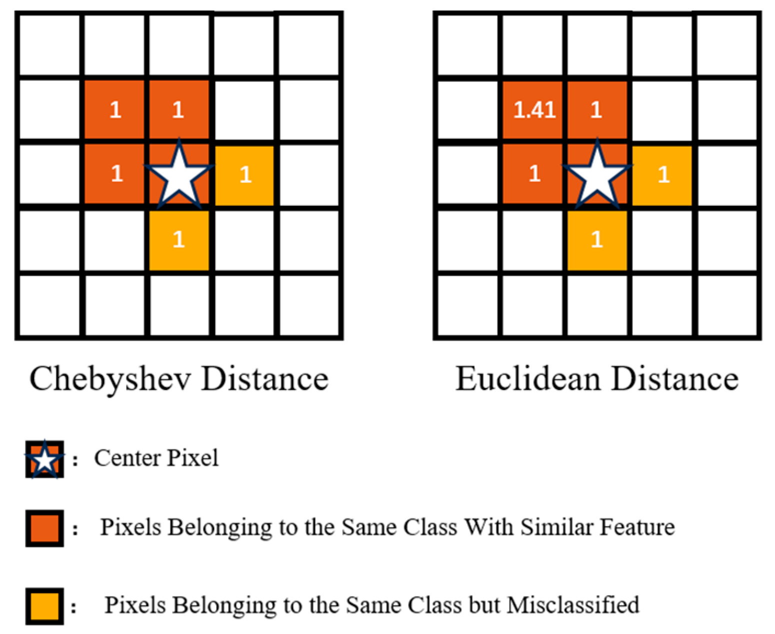
In contrast to that done in other methods, we did not choose the commonly used Euclidean geometric distance to calculate geographical distance. This is because a feature is typically distributed at the pixel level of an image in a continuous regular shape (e.g., a rectangle) rather than a discrete distribution [61,62].
Figure 2 shows that pixels similar to the right of the central reference pixel were misclassified into the same category using unsupervised classification. Suppose the spatial weights are calculated according to the Euclidean geometric distance; then, the misclassified pixels have higher spatial weights than similar pixels belonging to the same feature type in the upper-left diagonal. Suppose the spatial weights are calculated using the Chebyshev distance; then, the spatial weights of both are the same, and the exact contribution is left to the spectral weights to determine, which reduces the influence of misclassified pixels on the results of predicting the missing pixels.

2.3.2. Spectral Weight

For spectral weighting, we measured the spectral similarity of a pixel similar to the center reference pixel using the spectral angle mapper method, which determines the spectral similarity between two pixels by calculating the angle between their spectral feature vectors.
D S A M ( T ) = cos 1 T v R v T v T v 1 2 R v R v 1 2
where T v is the center reference pixel feature vector, and R v is the similar pixel feature vector. T v and R v represent their transpose vectors, respectively.
Because the values of different features in a certain band may be approximate, a small fraction of the pixels of other feature classes are likely to be misclassified into the same feature class as the center reference pixel when performing unsupervised classification. Therefore, we approximately took the four bands of the center reference and similar pixels as their spectral feature curves and simultaneously constructed a 3 × 3 (or 5 × 5) block centered on each of them as a shape feature, which can be used to determine whether both genuinely belong to the same feature classification.

2.4. Predicting Missing Pixel Values

A simple least-squares linear fitting is applied to predict each missing pixel value, i.e.,
T ( x , y , b ) = α × R ( x , y , b ) + β
where R x ,   y ,   b and T x ,   y ,   b represent the pixels at location x , y in band b in the reference image and the target image. α and β are the slope and intercept of the linear regression.
We rank the similar pixels according to the product of the spatial weights and spectral weights from highest to lowest. In this study, the first 50 similar pixels having the highest weight are selected to predict the missing pixel. α and β are obtained by (5) using the similar pixels and the pixels at the corresponding positions of the target image. Finally, the value of the missing pixel can be predicted by substituting the center pixel into (5).

3. Results

3.1. Simulated Experiments

To evaluate the recovery effect of SAIW filling in the present study, we artificially applied an irregular mask to the GF-1 WFV images to simulate a region with missing pixel values owing to cloud cover. We used the original pixel values of the region as validation data to test the effectiveness and accuracy of the proposed method.
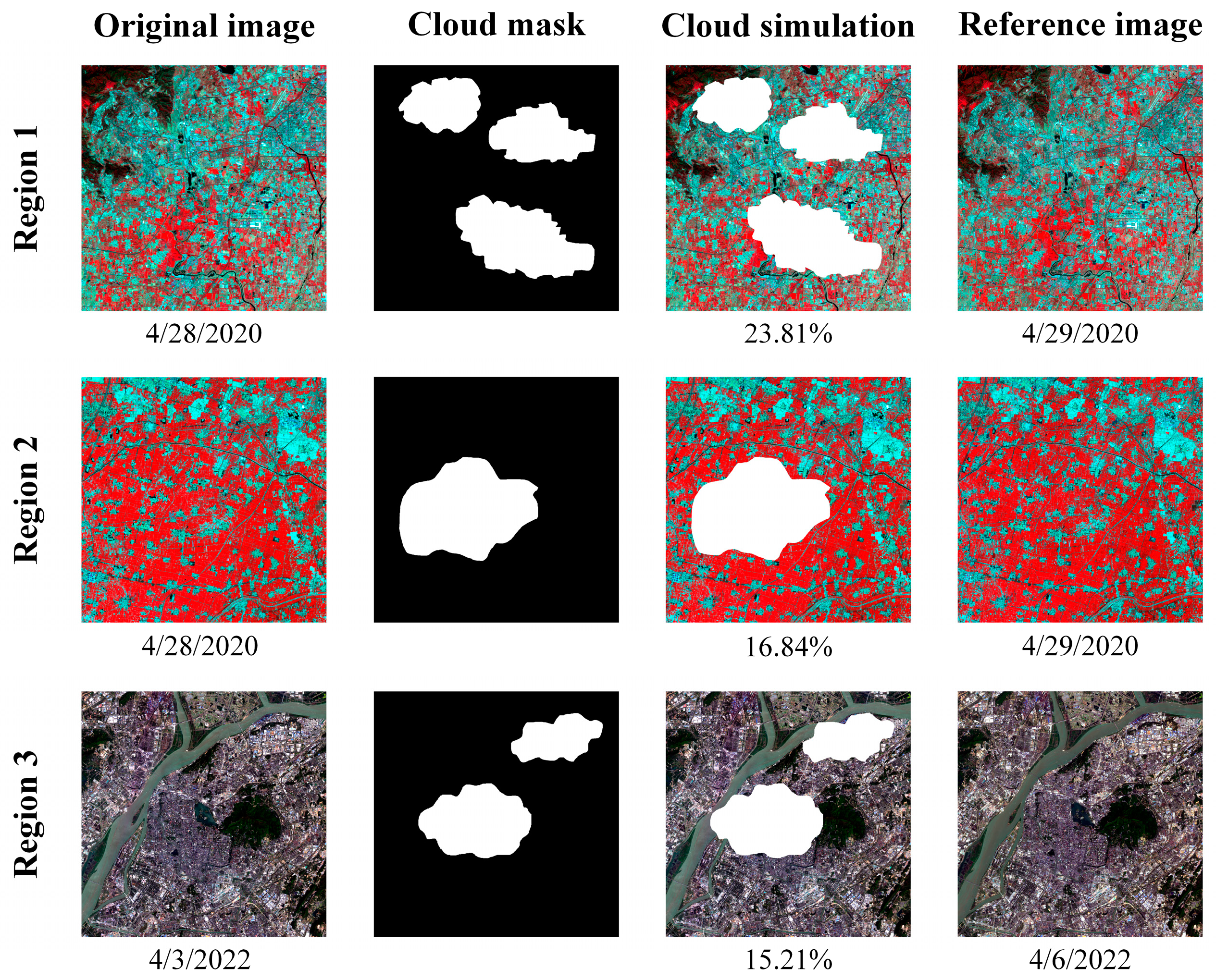
We selected three regions with characteristic land cover types for the experiments (Figure 3). Each region used two images: a simulated cloud-contaminated image and a reference image. The first experimental region was selected in southwest Beijing, which has various land cover types, including urban areas, farmland, bare soil, water, and mountains. Cloud-simulated and reference images were acquired on 28–29 April 2020. The second experimental area is located in the North China Plain, where the land cover types are mainly farmland, and the selected cloud simulation images and reference images were acquired at the same time as the first experimental area, that is, 28–29 April 2020, respectively. To test the filling effect of the proposed method in dense urban areas, the third experimental region was set in Nanjing City, and the cloud simulation and reference images acquired on 3–6 April 2022, were selected.
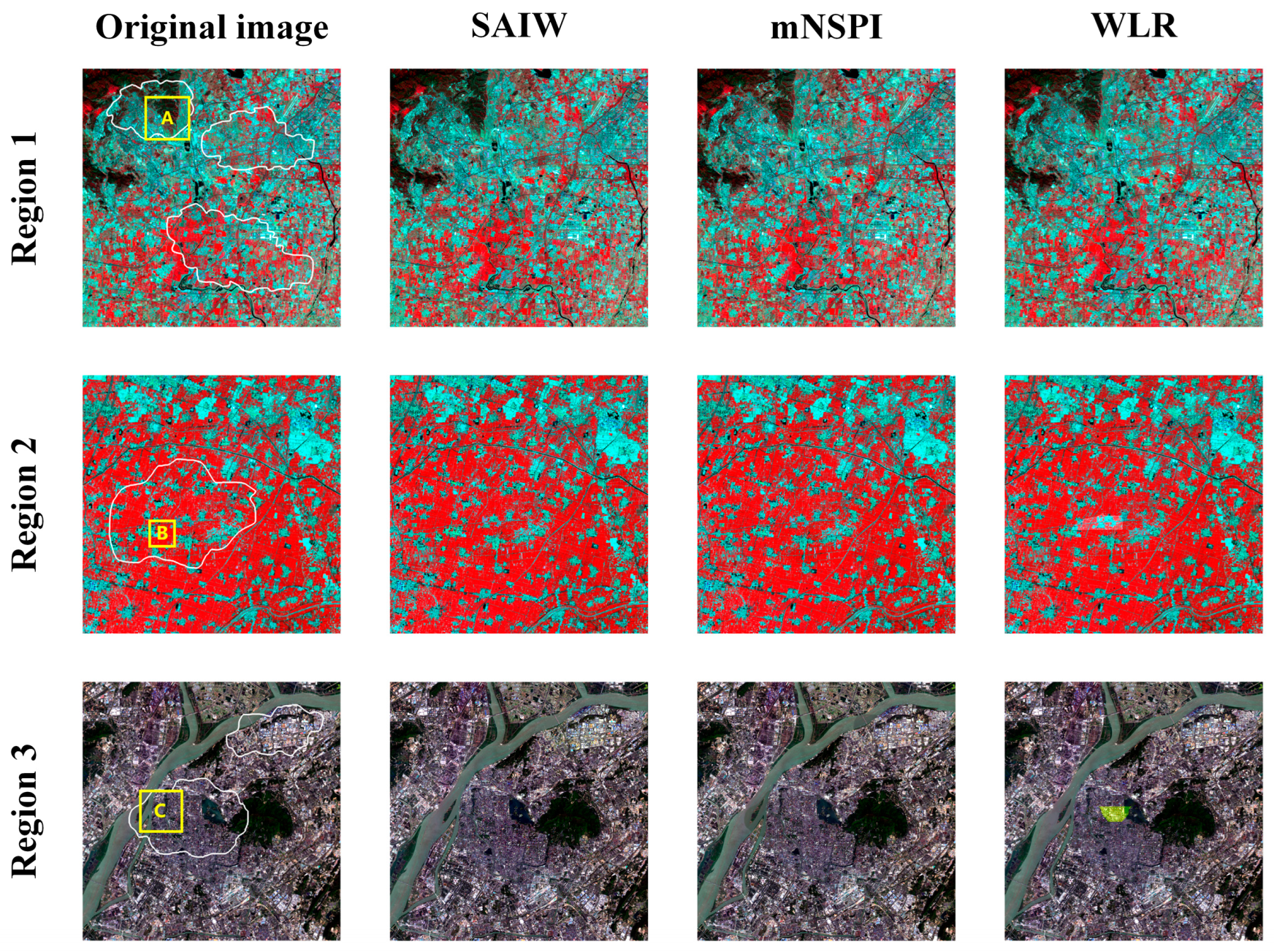
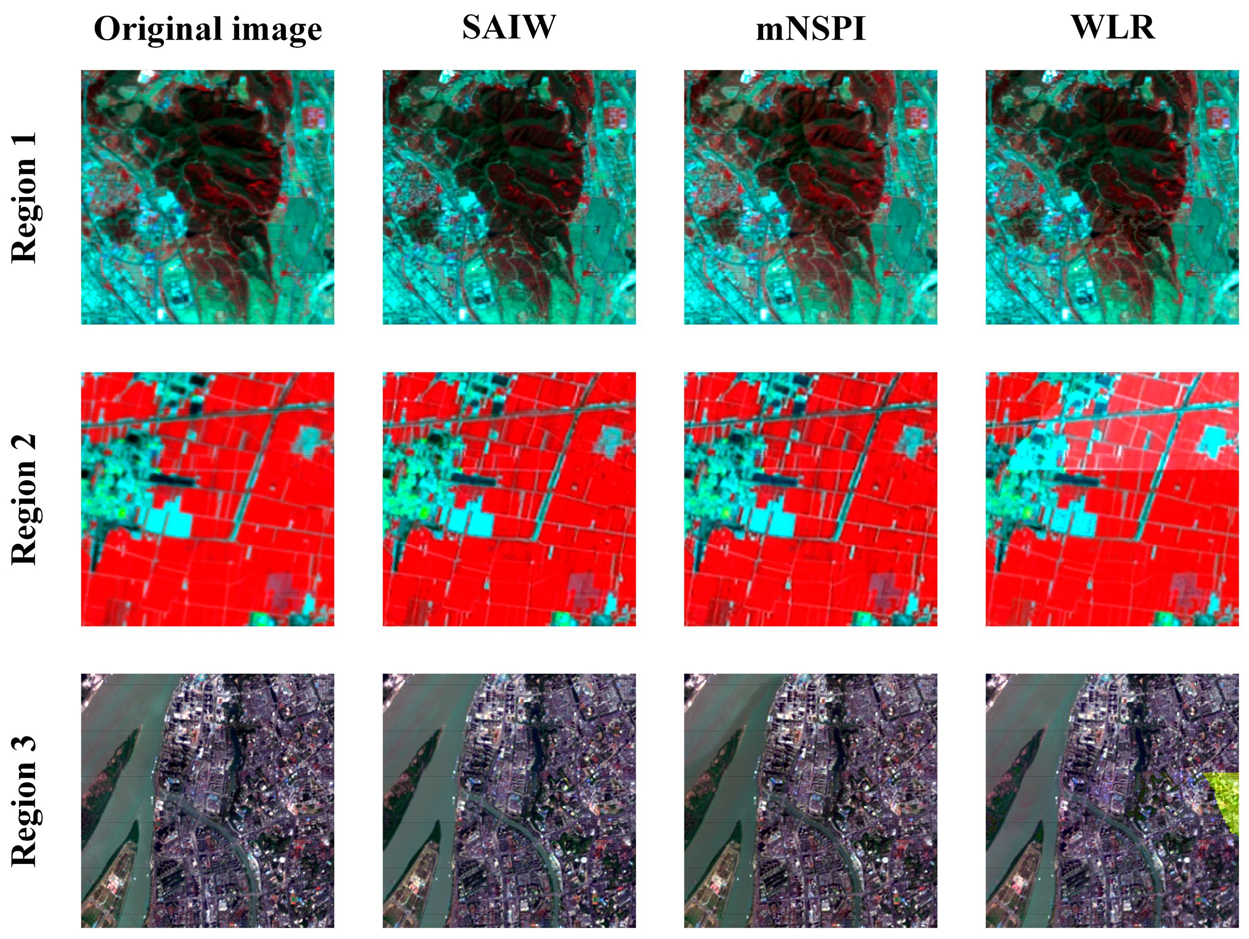
The results of the proposed SAIW method were compared with those obtained using a modified neighborhood similar pixel interpolator (mNSPI) [35] and linear weighted regression (WLR) [36] on the original images. Specifically, mNSPI combines spectral-spatial and spectral-temporal information to predict missing pixels. WLR reconstructs missing pixels based on locally similar pixels using weighted linear regression. mNSPI and WLR use Euclidean and spectral distances to compute spatial and spectral weights, with mNSPI utilizing the difference in spectral values to determine the size of the search window and WLR using a fixed window size. The filling results of the proposed method, mNSPI, and WLR are shown in Figure 4. The three sub-regions of the study area were enlarged to show the differences in the results between the methods (Figure 5).
The primary land cover type in sub-region A was mountainous. The SAIW method had a good visual effect of filling in the mountainous area; the mNSPI method filled in the overall reddish result, which is also caused by the high NIR value as the red band displayed, low contrast at the shadows of the mountain, and the area covered by vegetation being too apparent. The WLR method was not suitable for recovering detailed parts of ridges and valleys with patches.
The primary surface cover type in sub-region B was agricultural land. In this experiment, SAIW and mNSPI showed satisfactory visual results. However, a white blocky noise area was observed in the WLR results. The quantitative metrics of the SAIW method-filled results indicated that they were closer to the original images than those of mNSPI and WLR, maintaining good spectral consistency while retaining more spatial information allowing SAIW to predict the missing data more accurately.
Sub-region C was a complex urban area. SAIW retained some urban architectural details in this heterogeneous region and achieved better filling results. The mNSPI also retained good architectural details in the filling result but did not match the original image in the water portion. The WLR had the same results as in Region 2, with blocky noise areas and some blurring of the dense architectural areas. In the same way, the quantitative evaluation of the SAIW fill results was the best among all methods, confirming that the SAIW method can provide high-quality fill in complex urban areas.
We calculated the Pearson’s correlation coefficient (R) and root mean square error (RMSE), which are accuracy indicators of the predicted and observed reflectance of the missing region. The results of the accuracy evaluation are presented in Table 2. The results showed that the proposed method outperformed the other two research methods in terms of R and RMSE for all four bands, with the highest correlation in the visible bands (red, green, and blue), and the accuracy in the NIR bands was slightly lower than that in the other three bands. The quantitative metrics showed the same regularity for all three methods, a phenomenon that may be due to sensor differences between the Landsat 8 OLI and GF-1 WFV. Overall, the accuracy evaluation metrics indicated that the proposed method had a lower prediction bias than mNSPI and WLR and that its predictions were closer to the original images.

3.2. Impact of Reference Images Obtained at Different Times on the Accuracy of Simulated Experiments

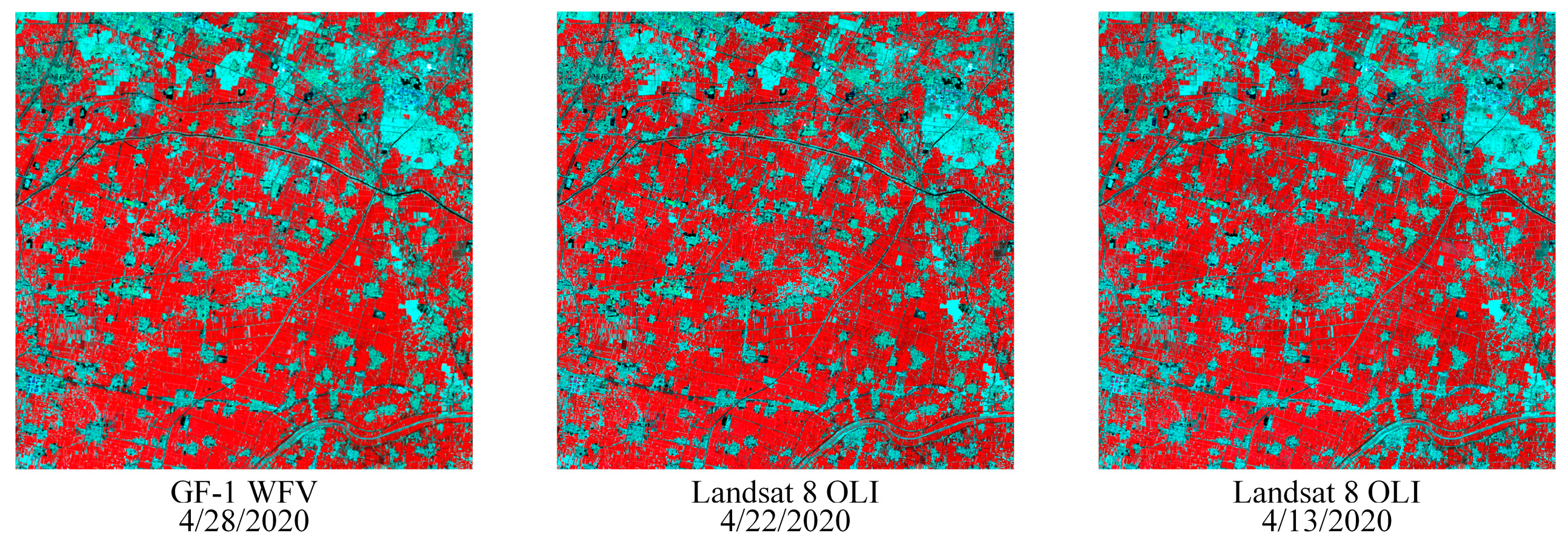
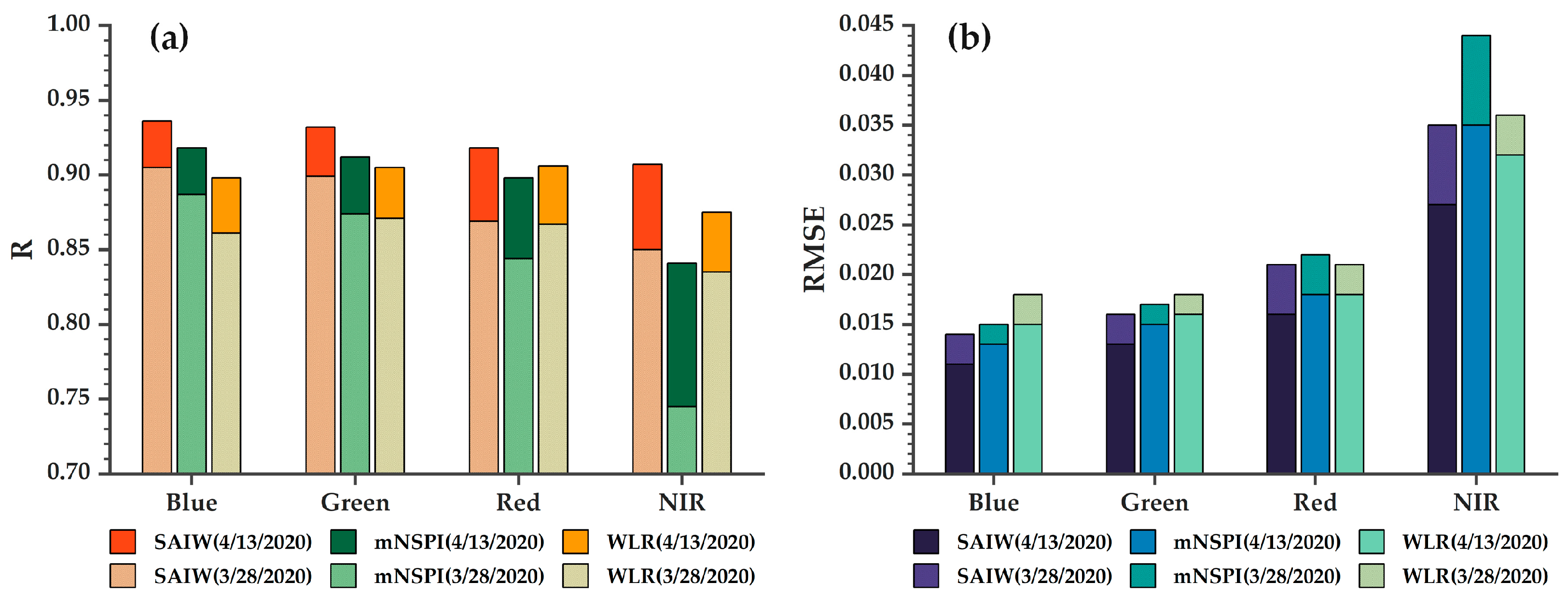
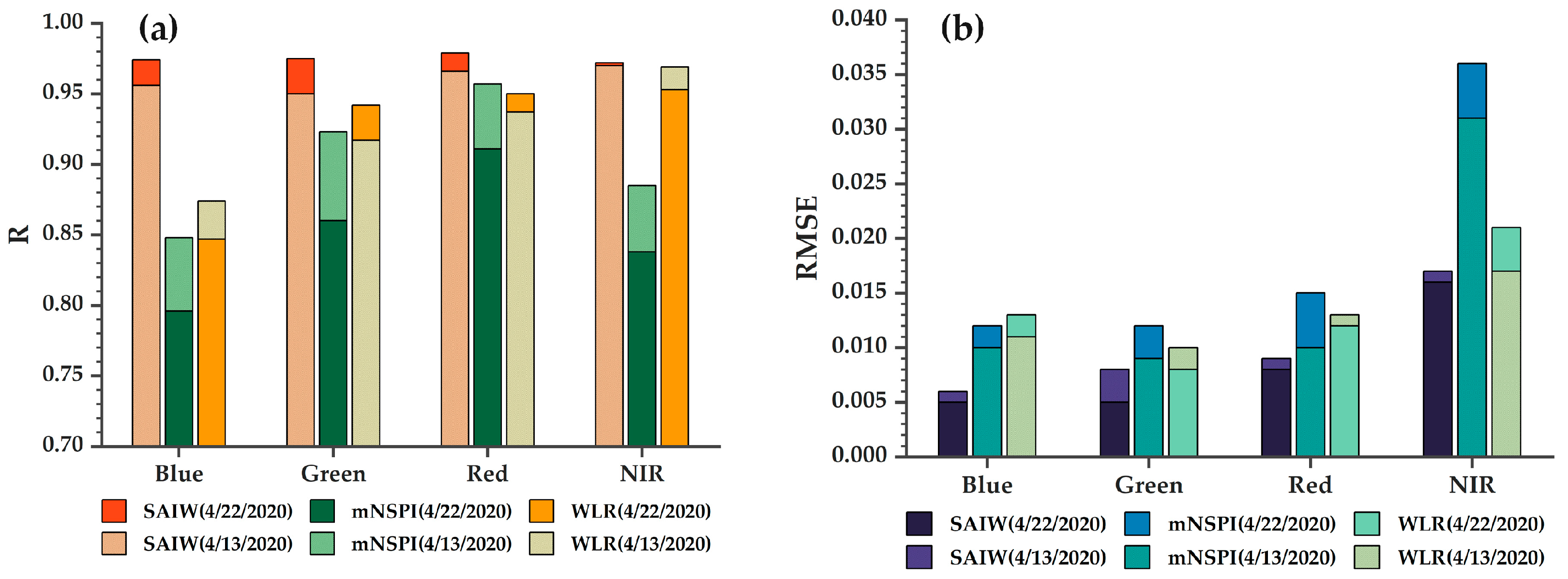
As the temporal distance between the reference and cloudy images increases, the surface reflectance at the same location changes significantly owing to seasonal variations, which can substantially impact the filling accuracy. To reveal this effect, we analyzed the sensitivity of the performance of the SAIW, mNPSI, and WLR methods to the time of acquisition of the reference image. To illustrate this issue, we tested it in southwest Beijing (Region 1) and the North China Plain (Region 2). The dates of the reference images chosen in Section 3.1 for both regions are only one day away from the target image. For this reason, we selected images from 13 April 2020 (15 days away) and 28 March 2020 (31 days away) for southwest Beijing (Figure 6), and 22 April 2020 (6 days away) and 13 April 2020 (15 days away) for the North China Plain (Figure 7).
In southwest Beijing, when the correlation of all three methods decreased to a certain extent with increasing temporal distance, the complex surface cover types and climatic variations caused the target image and reference time to show apparent visual differences. In general, the prediction accuracy of SAIW is always greater than that of mNSPI and WLR, and satisfactory prediction results can be achieved in regions with complex surface cover types (Figure 8).
The North China Plain is a homogeneous region in which winter wheat is the predominant land cover type [63]. Winter wheat is in the jointing and booting stages from mid to late April [64]. During these stages, the reflectance of visible light (especially in the green band) and NIR light decreases gradually [65,66]. The accuracy of SAIW was less affected by the change in the reflectance, particularly in the NIR band (the correlation of the NIR band on 22 and 13 April only decreased by 0.010 and 0.012, respectively, compared with that on 28 April) (Figure 9). By contrast, the mNSPI and WLR accuracies decreased slightly.

3.3. Impact of Cloud Sizes on the Accuracy of Simulated Experiments

In this section, we analyze the performance of the proposed method in terms of cloud size. Irregular cloud masks of different sizes were applied to the images of southwest Beijing as experimental data (Figure 10).
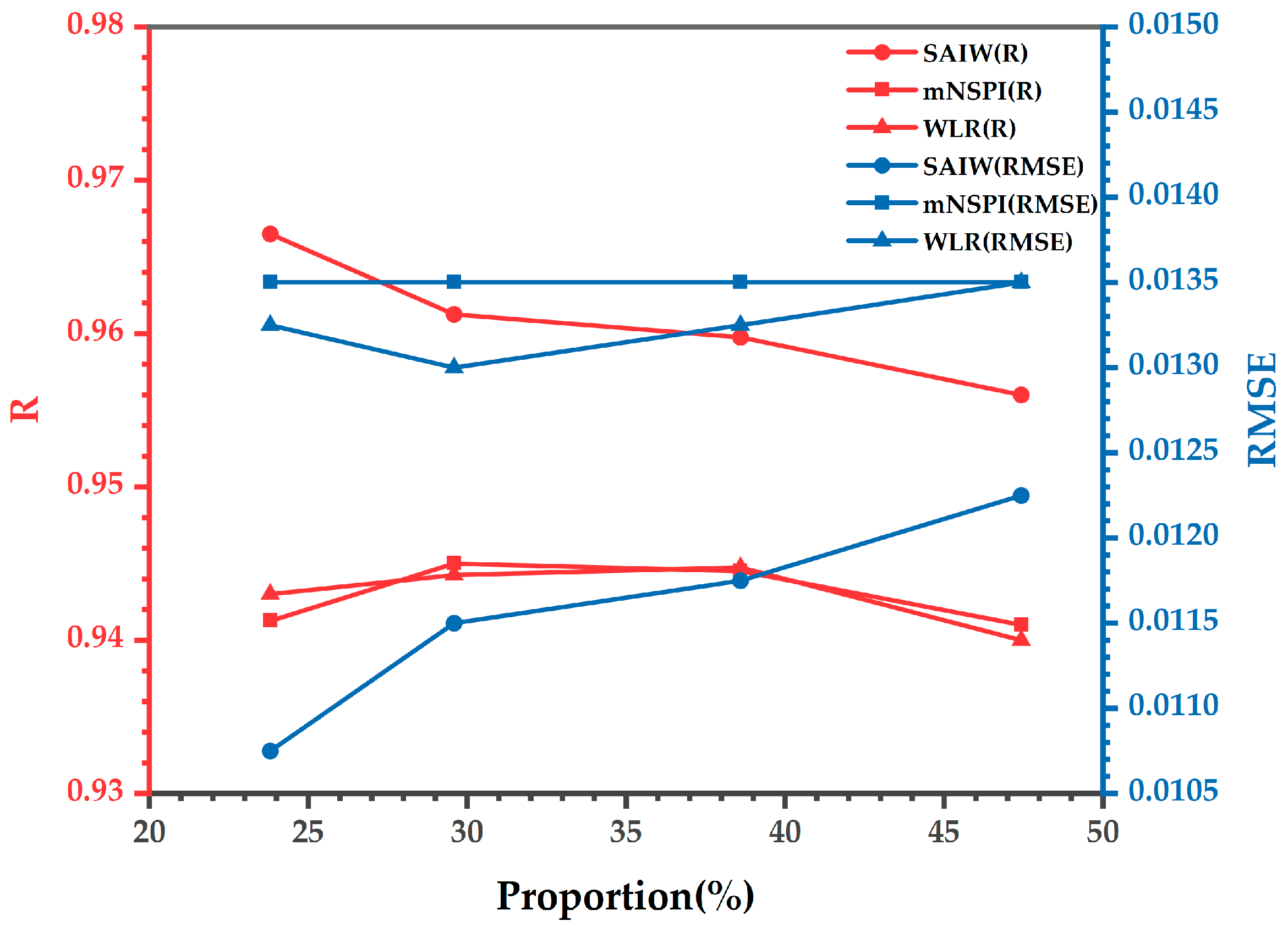
We calculated the average correlation coefficients for the SAIW, mNSPI, and WLR across four bands to reflect the trend in accuracy of the results under cloud cover of different sizes (Figure 11). The proposed SAIW method showed the highest accuracy (i.e., it usually had the highest R and lowest RMSE values in all bands) for cloud-covered areas of different sizes among the three methods (Table 3). The smaller the cloud coverage area, the more pronounced the advantage of the proposed SAIW method. The correlation coefficient R of the SAIW method still showed better accuracy than the other two methods when the size of the cloud-covered area increased to 47.43% of the entire image.

3.4. Real Data Experiments

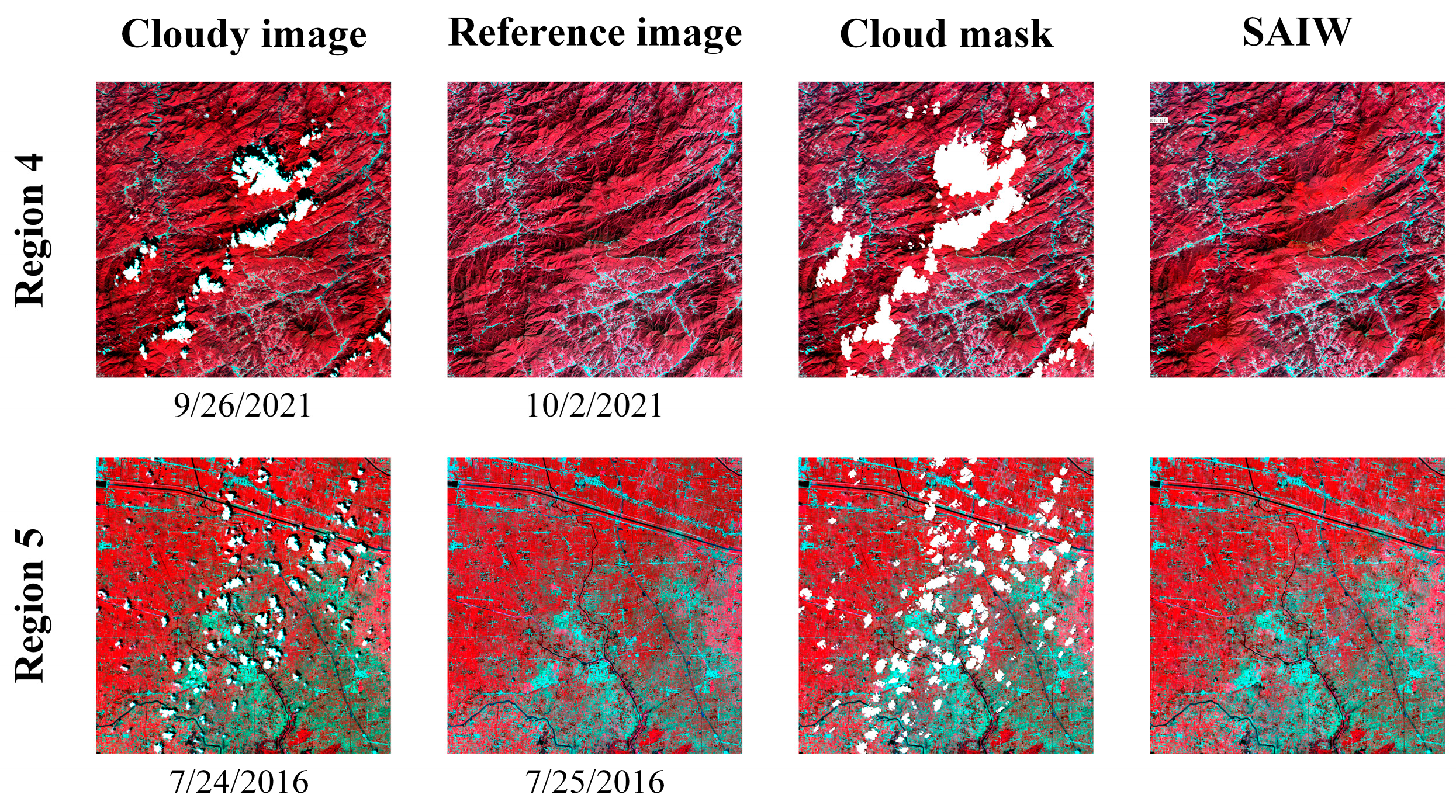
To further validate the performance of the SAIW method and prove that SAIW can indeed be used to fill areas covered by real clouds, two sets of GF-1 WFV real-data experiments were conducted separately. The first set of experiments was based on an image of a mountainous area (Region 4) near Wuhan, Hubei Province, which was cloud-covered on 26 September 2021, and a Landsat 8 OLI image was obtained on 2 October 2021. The second set of experiments was based on a cloud-contaminated image (Region 5) obtained on 24 July 2016, in the Yangtze River Delta region, with the Landsat 8 OLI data obtained on 25 July 2016, as the reference image, which was mainly used to test the actual filling effect of the SAIW method in the agricultural area.
The filling results are shown in Figure 12. For a visual comparison, we applied a cloud mask to a real cloudy image (third column in Figure 12) to eliminate the effect of clouds on the real color of the image. The results showed that the SAIW predictions in the two regions had attractive visual continuity and relatively harmonious hues, indicating that the SAIW performed satisfactorily in removing real clouds from the GF-1 WFV data.

4. Discussion

The Landsat 8 OLI images are used as a reference image for GF-1 WFV image gap filling, which reaped satisfactory results in the experiment. When using Landsat 8 OLI images to fill in the gaps in the GF-1 WFV images, we have to consider the problem of spatial resolution difference. For the purpose of downscaling the Landsat 8 OLI to the same spatial resolution as the GF-1 WFV, the method in the PCI Geomatics Banff 2020 SP2 software named the PANSHARP was used to downscale [67]. The sharpened images were resampled to 16 m to maintain the consistent spatial resolution as GF-1 WFV. This measure is demonstrated to be efficacious in preserving the integrity of detailed features within the result of gap fill, notwithstanding that the pan-sharpening fusion process causes deviations in pixel values. However, utilizing the Landsat 8 OLI image, which has been directly resampled to 16-m resolution, as a reference image for filling the GF-1 WFV image will lead to a needless smoothing effect in the reconstructed areas. This points to the critical necessity for a critical pan-sharpening fusion and resampling strategy in order to retain the high-resolution detail that is characteristic of the target image. Given that Sentinel-2 offers a spatial resolution of 10 m across all visible bands, it was initially considered as a potential choice of reference image [68,69]. However, despite its spatial resolution being relatively close to that of the GF-1 WFV, the filling results within the NIR band reveal inconsistencies in feature continuity along the boundaries of the targeted area. This is attributed to Sentinel-2’s spatial resolution in the NIR band being 20 m, which introduces discrepancies at the edges when used for gap filling [70].
The proposed method quantifies the spatial correlation within the search window using Getis-Ord Gi* as a metric and determines the optimal search window size based on the highest spatial autocorrelation. This strategy makes full use of the spatial correlation between the neighboring pixels and the central reference pixel. The adaptive search window strategy ensures a sufficient number of similar pixels, thereby facilitating the precise reconstruction of missing pixels and enriching the detail within the filling results. Typically, the reconstruction of missing pixels is performed on a pixel-by-pixel basis [71,72], with each sequentially reconstructed pixel contributing as a candidate of a similar pixel in the ensuing calculation of the next similar missing pixel, thus iteratively influencing subsequent results [73]. This means that the selectable similar pixels for a missing pixel at the same position that can be selected are dynamic, contingent upon the sequence of computation—whether it progresses in a row-by-row order, a row-by-row reverse order, a column-by-column order, or a column-by-column reverse order [74]. Therefore, it warrants further investigation to assess the comparative results of pixel reconstruction from varying orientations and their impact on accuracy. Moreover, it would be worthwhile to explore the potential impact on accuracy and computational efficiency of gap filling from four cardinal directions concurrently.
Improved spatial and spectral weights reduce the misjudgment of similar pixels due to unsupervised classification and enhance the feature information of similar pixels in the neighborhood window. In contrast to that in mNSPI and WLR, the weights of similar pixels are computed in SAIW to conveniently filter pixels that are correlated with the central reference pixel. The weights of the pixels were not involved in the prediction of the missing pixels. Linear fitting was used to represent the temporally varying relationship between the missing pixels and the central reference pixel. The proposed method provides a simple concept of the gap-filling method.
Notably, the selection and further screening of similar pixels are mainly determined by the information of the reference image, which means that when there is a large difference between the land cover type of the reference image and the target image or when there is a sudden change in the land cover type within a short time, the cloud-covered region in the cloudy image cannot be predicted accurately. Therefore, as in most previously proposed multi-temporal gap-filling methods [75,76,77], SAIW is suitable for situations where the time intervals are relatively short or land cover changes are not obvious.
We ran all the methods on a PC configured with Intel Core i5-11400 CPU and 32 GB RAM. As an example, the time required to process 54,020 pixels in a 1506 × 1506 resolution image is about 22 min for the SAIW method to run, about 18 min for mNSPI, and about 13 min for WLR. Although the SAIW method outperforms both of the other two methods in reconstructing missing pixels, this is obtained at the expense of computational efficiency. The main loss in computational efficiency is in the process of determining similar pixels and windows for each pixel. Because of the use of the adaptive windowing strategy, a spatial autocorrelation calculation will be performed once for each alternative search window size for each missing pixel to determine the search window size. Also, the calculation of spectral weights is oriented towards the calculation of arrays, which will take up more computational resources than numerical calculations. To enhance computational efficiency, future research will investigate the strategy of segmenting the missing area within the same spectral band to enable simultaneous computation. Additionally, there will be efforts to perform computations across multiple bands concurrently for the missing pixels.
Currently, only one reference image is used as the secondary source of information. In future studies, we will attempt to obtain information from images at different time intervals simultaneously, making the gap-filling method applicable to situations where the land cover type changes. With the advent of additional satellite deployments and the increasing of available medium- and high-resolution images, reference images from multiple sources will be used in future studies to be incorporated into the gap-filling process, rendering the proposed method more adept at the reconstruction of cloud-polluted areas with sudden changes in surface cover. In the application of multi-source remote sensing images for gap-filling purposes, the differences between sensors will be considered. It is aimed at reducing the propagation of errors within the gap-filling process, thereby significantly improving the accuracy of filling results.

5. Conclusions

The SAIW method fills cloud-covered regions in the target image by utilizing information from reference images at adjacent times. This process involves a series of steps, including adaptively determining the size of the search window, along with selecting and screening similar pixels. Specifically, the Getis-Ord Gi* metric was employed to establish the spatial correlation between the pixels within the window and the central pixel, facilitating the selection of an appropriate window size. Subsequently, the spatial and spectral information of similar pixels was calculated using the Chebyshev distance and spectral angle mapper, respectively, to optimize the spatial and spectral weights. Finally, the missing pixels were predicted based on filtered similar pixels using linear fitting. This can reduce the spread of errors in the gap-filling process, significantly improving the accuracy of the filling results. To demonstrate the advantages of the SAIW method, simulation experiments were conducted in different study areas to verify the filling performance of the SAIW method under typical surface cover types. The effects of different cloud area sizes and time intervals between the reference and target images on the accuracy of the fill process were analyzed. Good visual filling effects were observed in the experiments with real cloud-contaminated images, which proved that the use of the SAIW method to fill GF-1 WFV images was reliable.

Author Contributions

Conceptualization, T.C. and T.Y.; methodology, T.C., L.Z., X.M. and Y.L.; software, T.C.; validation, T.C., W.Z. and Y.Z.; formal analysis, T.C., X.M. and Y.L.; investigation, T.C. and T.Y.; resources, T.Y. and J.Y.; data curation, C.W. and J.L.; writing—original draft preparation, T.C. and L.Z.; writing—review and editing, T.C., L.Z. and W.Z.; visualization, T.C.; supervision, C.W., Y.Z. and J.L.; project administration, T.Y., L.Z. and J.Y.; funding acquisition, T.Y. and L.Z. All authors have read and agreed to the published version of the manuscript.

Funding

This research was funded by the National Key R&D Program of China (2021YFE0117300), Common Application Support Platform for National Civil Space Infrastructure Land Observation Satellites (2017-000052-73-01-001735), the Major Project of High Resolution Earth Observation System (30-Y60B01-9003-22/33), the Natural Science Foundation of Hebei Province (D2022103002), and the Natural Science Foundation of Hainan Province (423MS113).

Institutional Review Board Statement

Not applicable.

Informed Consent Statement

Not applicable.

Data Availability Statement

The Gaofen-1 (GF-1) wide-field viewer (WFV) L1A data can be accessed at the China Center for Resources Satellite Data and Application (CRESDA): https://data.cresda.cn/#/home (accessed on 10 February 2023). The Landsat-8 surface reflectance data can be accessed at the United States Geological Survey (USGS): https://glovis.usgs.gov/app (accessed on 10 February 2023).

Acknowledgments

The authors would like to thank Xiaolin Zhu and Huanfeng Shen for making the source codes of mNSPI and WLR publicly available. Appreciation is also extended to the anonymous reviewers for their careful review and constructive suggestions to improve the manuscript.

Conflicts of Interest

The authors declare no conflicts of interest.

References

  1. Toth, C.; Jóźków, G. Remote sensing platforms and sensors: A survey. ISPRS J. Photogramm. Remote Sens. 2016, 115, 22–36. [Google Scholar] [CrossRef]
  2. Jiménez-Jiménez, S.I.; Ojeda-Bustamante, W.; Ontiveros-Capurata, R.E.; Marcial-Pablo, M.D.J. Rapid urban flood damage assessment using high resolution remote sensing data and an object-based approach. Geomat. Nat. Hazards Risk 2020, 11, 906–927. [Google Scholar] [CrossRef]
  3. Gibson, R.; Danaher, T.; Hehir, W.; Collins, L. A remote sensing approach to mapping fire severity in south-eastern Australia using sentinel 2 and random forest. Remote Sens. Environ. 2020, 240, 111702. [Google Scholar] [CrossRef]
  4. Taftsoglou, M.; Valkaniotis, S.; Papathanassiou, G.; Karantanellis, E. Satellite Imagery for Rapid Detection of Liquefaction Surface Manifestations: The Case Study of Türkiye–Syria 2023 Earthquakes. Remote Sens. 2023, 15, 4190. [Google Scholar] [CrossRef]
  5. Zhu, Q.; Guo, X.; Deng, W.; Shi, S.; Guan, Q.; Zhong, Y.; Zhang, L.; Li, D. Land-use/land-cover change detection based on a Siamese global learning framework for high spatial resolution remote sensing imagery. ISPRS J. Photogramm. Remote Sens. 2022, 184, 63–78. [Google Scholar] [CrossRef]
  6. Tong, X.Y.; Xia, G.S.; Lu, Q.; Shen, H.; Li, S.; You, S.; Zhang, L. Land-cover classification with high-resolution remote sensing images using transferable deep models. Remote Sens. Environ. 2020, 237, 111322. [Google Scholar] [CrossRef]
  7. Li, D.; Wang, M.; Jiang, J. China’s high-resolution optical remote sensing satellites and their mapping applications. Geo-Spat. Inf. Sci. 2021, 24, 85–94. [Google Scholar] [CrossRef]
  8. Chen, L.; Letu, H.; Fan, M.; Shang, H.; Tao, J.; Wu, L.; Zhang, Y.; Yu, C.; Gu, J.; Zhang, N.; et al. An introduction to the Chinese high-resolution Earth observation system: Gaofen-1~7 civilian satellites. J. Remote Sens. 2022, 2022, 9769536. [Google Scholar] [CrossRef]
  9. Xu, K.; Tian, Q.; Zhang, Z.; Yue, J.; Chang, C.-T. Tree Species (Genera) Identification with GF-1 Time-Series in A Forested Landscape, Northeast China. Remote Sens. 2020, 12, 1554. [Google Scholar] [CrossRef]
  10. Li, J.; Mao, X. Comparison of Canopy Closure Estimation of Plantations Using Parametric, Semi-Parametric, and Non-Parametric Models Based on GF-1 Remote Sensing Images. Forests 2020, 11, 597. [Google Scholar] [CrossRef]
  11. Song, Q.; Hu, Q.; Zhou, Q.; Hovis, C.; Xiang, M.; Tang, H.; Wu, W. In-Season Crop Mapping with GF-1/WFV Data by Combining Object-Based Image Analysis and Random Forest. Remote Sens. 2017, 9, 1184. [Google Scholar] [CrossRef]
  12. Wu, M.; Zhang, X.; Huang, W.; Niu, Z.; Wang, C.; Li, W.; Hao, P. Reconstruction of Daily 30 m Data from HJ CCD, GF-1 WFV, Landsat, and MODIS Data for Crop Monitoring. Remote Sens. 2015, 7, 16293–16314. [Google Scholar] [CrossRef]
  13. Li, H.; Liu, G.; Liu, Q.; Chen, Z.; Huang, C. Retrieval of Winter Wheat Leaf Area Index from Chinese GF-1 Satellite Data Using the PROSAIL Model. Sensors 2018, 18, 1120. [Google Scholar] [CrossRef]
  14. Lu, S.; Deng, R.; Liang, Y.; Xiong, L.; Ai, X.; Qin, Y. Remote Sensing Retrieval of Total Phosphorus in the Pearl River Channels Based on the GF-1 Remote Sensing Data. Remote Sens. 2020, 12, 1420. [Google Scholar] [CrossRef]
  15. Chen, Y.L.; Wan, J.H.; Zhang, J.; Ma, Y.J.; Wang, L.; Zhao, J.H.; Wang, Z.Z. Spatial-temporal distribution of golden tide based on high-resolution satellite remote sensing in the South Yellow Sea. J. Coast. Res. 2019, 90, 221–227. [Google Scholar] [CrossRef]
  16. Zhong, B.; Chen, W.; Wu, S.; Hu, L.; Luo, X.; Liu, Q. A cloud detection method based on relationship between objects of cloud and cloud-shadow for Chinese moderate to high resolution satellite imagery. IEEE J. Sel. Top. Appl. Earth Obs. Remote Sens. 2017, 10, 4898–4908. [Google Scholar] [CrossRef]
  17. Shen, H.; Li, X.; Cheng, Q.; Zeng, C.; Yang, G.; Li, H.; Zhang, L. Missing Information Reconstruction of Remote Sensing Data: A Technical Review. IEEE Geosci. Remote Sens. Mag. 2015, 3, 61–85. [Google Scholar] [CrossRef]
  18. Zhang, C.; Li, W.; Travis, D. Gaps-fill of SLC-off Landsat ETM+ satellite image using a geostatistical approach. Int. J. Remote Sens. 2007, 28, 5103–5122. [Google Scholar] [CrossRef]
  19. Sekulić, A.; Kilibarda, M.G.B.; Heuvelink, M.; Nikolić, M.; Bajat, B. Random forest spatial interpolation. Remote Sens. 2020, 12, 1687. [Google Scholar] [CrossRef]
  20. Zhuang, L.; Bioucas-Dias, J.M. Fast Hyperspectral Image Denoising and Inpainting Based on Low-Rank and Sparse Representations. IEEE J. Sel. Top. Appl. Earth Obs. Remote Sens. 2018, 11, 730–742. [Google Scholar] [CrossRef]
  21. Chen, Y.; He, W.; Yokoya, N.; Huang, T.Z. Blind cloud and cloud shadow removal of multitemporal images based on total variation regularized low-rank sparsity decomposition. ISPRS J. Photogramm. Remote Sens. 2019, 157, 93–107. [Google Scholar] [CrossRef]
  22. Huang, Z.; Zhang, Y.; Li, Q.; Li, X.; Zhang, T.; Sang, N.; Hong, H. Joint Analysis and Weighted Synthesis Sparsity Priors for Simultaneous Denoising and Destriping Optical Remote Sensing Images. IEEE Trans. Geosci. Remote Sens. 2020, 58, 6958–6982. [Google Scholar] [CrossRef]
  23. Shen, H.; Wu, J.; Cheng, Q.; Aihemaiti, M.; Zhang, C.; Li, Z. A spatiotemporal fusion based cloud removal method for remote sensing images with land cover changes. IEEE J. Sel. Top. Appl. Earth Obs. Remote Sens. 2019, 12, 862–874. [Google Scholar] [CrossRef]
  24. Zhu, S.; Li, Z.; Shen, H.; Lin, D. A fast two-step algorithm for large-area thick cloud removal in high-resolution images. Remote Sens. Lett. 2023, 14, 1–9. [Google Scholar] [CrossRef]
  25. Jia, A.; Wang, D.; Liang, S.; Peng, J.; Yu, Y. Global daily actual and snow-free blue-sky land surface albedo climatology from 20-year MODIS products. J. Geophys. Res. Atmos. 2022, 127, e2021JD035987. [Google Scholar] [CrossRef]
  26. Jia, A.; Wang, D.; Liang, S.; Peng, J.; Yu, Y. Improved cloudy-sky snow albedo estimates using passive microwave and VIIRS data. ISPRS J. Photogramm. Remote Sens. 2023, 196, 340–355. [Google Scholar] [CrossRef]
  27. Chen, Y.; Cao, R.; Chen, J.; Liu, L.; Matsushita, B. A practical approach to reconstruct high-quality Landsat NDVI time-series data by gap filling and the Savitzky–Golay filter. ISPRS J. Photogramm. Remote Sens. 2021, 180, 174–190. [Google Scholar] [CrossRef]
  28. Sadeghi, M.; Behnia, F.; Amiri, R. Window Selection of the Savitzky–Golay Filters for Signal Recovery From Noisy Measurements. IEEE Trans. Instrum. Meas. 2020, 69, 5418–5427. [Google Scholar] [CrossRef]
  29. Yang, G.; Shen, H.; Zhang, L.; He, Z.; Li, X. A Moving Weighted Harmonic Analysis Method for Reconstructing High-Quality SPOT VEGETATION NDVI Time-Series Data. IEEE Trans. Geosci. Remote Sens. 2015, 53, 6008–6021. [Google Scholar] [CrossRef]
  30. Yang, Y.; Luo, J.; Huang, Q.; Wu, W.; Sun, Y. Weighted double-logistic function fitting method for reconstructing the high-quality sentinel-2 NDVI time series data set. Remote Sens. 2019, 11, 2342. [Google Scholar] [CrossRef]
  31. Zhao, J.; Zhang, X. An Adaptive Noise Reduction Method for NDVI Time Series Data Based on S–G Filtering and Wavelet Analysis. J. Indian Soc. Remote Sens. 2018, 46, 1975–1982. [Google Scholar]
  32. Rhif, M.; Ben Abbes, A.; Farah, I.R.; Martínez, B.; Sang, Y. Wavelet transform application for/in non-stationary time-series analysis: A review. Appl. Sci. 2019, 9, 1345. [Google Scholar] [CrossRef]
  33. Li, Z.; Shen, H.; Cheng, Q.; Li, W.; Zhang, L. Thick cloud removal in high-resolution satellite images using stepwise radiometric adjustment and residual correction. Remote Sens. 2019, 11, 1925. [Google Scholar] [CrossRef]
  34. Gerber, F.; de Jong, R.; Schaepman, M.E.; Schaepman-Strub, G.; Furrer, R. Predicting Missing Values in Spatio-Temporal Remote Sensing Data. IEEE Trans. Geosci. Remote Sens. 2018, 56, 2841–2853. [Google Scholar] [CrossRef]
  35. Zhu, X.; Gao, F.; Liu, D.; Chen, J. A Modified Neighborhood Similar Pixel Interpolator Approach for Removing Thick Clouds in Landsat Images. IEEE Geosci. Remote Sens. Lett. 2012, 9, 521–525. [Google Scholar] [CrossRef]
  36. Zeng, C.; Shen, H.; Zhang, L. Recovering missing pixels for Landsat ETM+ SLC-off imagery using multi-temporal regression analysis and a regularization method. Remote Sens. Environ. 2012, 131, 182–194. [Google Scholar] [CrossRef]
  37. Chen, B.; Huang, B.; Chen, L.; Xu, B. Spatially and Temporally Weighted Regression: A Novel Method to Produce Continuous Cloud-Free Landsat Imagery. IEEE Trans. Geosci. Remote Sens. 2017, 55, 27–37. [Google Scholar] [CrossRef]
  38. Yan, L.; Roy, D.P. Large-area gap filling of Landsat reflectance time series by spectral-angle-mapper based spatio-temporal similarity (SAMSTS). Remote Sens. 2018, 10, 609. [Google Scholar] [CrossRef]
  39. Jia, A.; Liang, S.; Wang, D. Generating a 2-km, all-sky, hourly land surface temperature product from Advanced Baseline Imager data. Remote Sens. Environ. 2022, 278, 113105. [Google Scholar] [CrossRef]
  40. Zhang, Q.; Yuan, Q.; Zeng, C.; Li, X.; Wei, Y. Missing data reconstruction in remote sensing image with a unified spatial–temporal–spectral deep convolutional neural network. IEEE Trans. Geosci. Remote Sens. 2018, 56, 4274–4288. [Google Scholar] [CrossRef]
  41. Jia, J.; Pan, M.; Li, Y.; Yin, Y.; Chen, S.; Qu, H.; Chen, X.; Jiang, B. GLTF-Net: Deep-Learning Network for Thick Cloud Removal of Remote Sensing Images via Global–Local Temporality and Features. Remote Sens. 2023, 15, 5145. [Google Scholar] [CrossRef]
  42. Zhao, Y.; Shen, S.; Hu, J.; Li, Y.; Pan, J. Cloud removal using multimodal GAN with adversarial consistency loss. IEEE Geosci. Remote Sens. Lett. 2021, 19, 1–5. [Google Scholar] [CrossRef]
  43. Wang, Y.; Zhou, X.; Ao, Z.; Xiao, K.; Yan, C.; Xin, Q. Gap-Filling and Missing Information Recovery for Time Series of MODIS Data Using Deep Learning-Based Methods. Remote Sens. 2022, 14, 4692. [Google Scholar] [CrossRef]
  44. Liu, M.; Liu, X.; Dong, X.; Zhao, B.; Zou, X.; Wu, L.; Wei, H. An improved spatiotemporal data fusion method using surface heterogeneity information based on ESTARFM. Remote Sens. 2020, 12, 3673. [Google Scholar] [CrossRef]
  45. Wang, Q.; Wang, L.; Wei, C.; Jin, Y.; Li, Z.; Tong, X.; Atkinson, P.M. Filling gaps in Landsat ETM+ SLC-off images with Sentinel-2 MSI images. Int. J. Appl. Earth Obs. Geoinf. 2021, 101, 102365. [Google Scholar] [CrossRef]
  46. Xia, M.; Jia, K. Reconstructing Missing Information of Remote Sensing Data Contaminated by Large and Thick Clouds Based on an Improved Multitemporal Dictionary Learning Method. IEEE Trans. Geosci. Remote Sens. 2022, 60, 5605914. [Google Scholar] [CrossRef]
  47. Brooks, E.B.; Wynne, R.H.; Thomas, V.A. Using window regression to gap-fill Landsat ETM+ post SLC-Off data. Remote Sens. 2018, 10, 1502. [Google Scholar] [CrossRef]
  48. Malambo, L.; Heatwole, C.D. A Multitemporal Profile-Based Interpolation Method for Gap Filling Nonstationary Data. IEEE Trans. Geosci. Remote Sens. 2016, 54, 252–261. [Google Scholar] [CrossRef]
  49. Zeng, C.; Shen, H.; Zhong, M.; Zhang, L.; Wu, P. Reconstructing MODIS LST Based on Multitemporal Classification and Robust Regression. IEEE Trans. Geosci. Remote Sens. 2015, 12, 512–516. [Google Scholar] [CrossRef]
  50. Yin, G.; Mariethoz, G.; McCabe, M.F. Gap-filling of landsat 7 imagery using the direct sampling method. Remote Sens. 2016, 9, 12. [Google Scholar] [CrossRef]
  51. Sadiq, A.; Edwar, L.; Sulong, G. Recovering the large gaps in Landsat 7 SLC-off imagery using weighted multiple linear regression (WMLR). Arabian J. Geosci. 2017, 10, 403. [Google Scholar] [CrossRef]
  52. Yan, L.; Roy, D.P. Spatially and temporally complete Landsat reflectance time series modelling: The fill-and-fit approach. Remote Sens. Environ. 2020, 241, 111718. [Google Scholar] [CrossRef]
  53. Cao, R.; Chen, Y.; Chen, J.; Zhu, X.; Shen, M. Thick cloud removal in Landsat images based on autoregression of Landsat time-series data. Remote Sens. Environ. 2020, 249, 112001. [Google Scholar] [CrossRef]
  54. Kandasamy, S.; Baret, F.; Verger, A.; Neveux, P.; Weiss, M. A comparison of methods for smoothing and gap filling time series of remote sensing observations–application to MODIS LAI products. Biogeosciences 2013, 10, 4055–4071. [Google Scholar] [CrossRef]
  55. Weiss, D.J.; Atkinson, P.M.; Bhatt, S.; Mappin, B.; Hay, S.I.; Gething, P.W. An effective approach for gap-filling continental scale remotely sensed time-series. ISPRS J. Photogramm. Remote Sens. 2014, 98, 106–118. [Google Scholar] [CrossRef] [PubMed]
  56. Liang, J.; Ren, C.; Li, Y.; Yue, W.; Wei, Z.; Song, X.; Zhang, X.; Yin, A.; Lin, X. Using Enhanced Gap-Filling and Whittaker Smoothing to Reconstruct High Spatiotemporal Resolution NDVI Time Series Based on Landsat 8, Sentinel-2, and MODIS Imagery. ISPRS Int. J. Geo-Inf. 2023, 12, 214. [Google Scholar] [CrossRef]
  57. Zhang, Y. Understanding image fusion. Photogramm. Eng. Remote Sens. 2004, 70, 657–661. [Google Scholar]
  58. Getis, A.; Ord, J.K. The analysis of spatial association by use of distance statistics. Geogr. Anal. 1992, 24, 189–206. [Google Scholar] [CrossRef]
  59. Ren, H.; Shang, Y.; Zhang, S. Measuring the spatiotemporal variations of vegetation net primary productivity in Inner Mongolia using spatial autocorrelation. Ecol. Indic. 2020, 112, 106108. [Google Scholar] [CrossRef]
  60. Karthik; Shivakumar, B.R. Land Cover Mapping Capability of Chaincluster, K-Means, and ISODATA Techniques—A Case Study. In Advances in VLSI, Signal Processing, Power Electronics, IoT, Communication and Embedded Systems: Select Proceedings of VSPICE 2020, 2nd ed.; Shubhakar, K., Muralidhar, K., Shivaprakasha, K.S., Eds.; Springer: Singapore, 2021; pp. 273–288. [Google Scholar]
  61. Suman, S.; Kumar, D.; Kumar, A. Study the Effect of MRF Model on Fuzzy c Means Classifiers with Different Parameters and Distance Measures. J. Indian Soc. Remote Sens. 2022, 50, 1177–1189. [Google Scholar] [CrossRef]
  62. Puzachenko, Y.G.; Sandlersky, R.B.; Krenke, A.N.; Olchev, A. Assessing the thermodynamic variables of landscapes in the southwest part of East European plain in Russia using the MODIS multispectral band measurements. Ecol. Modell. 2016, 319, 255–274. [Google Scholar] [CrossRef]
  63. Zhang, P.; Ma, W.; Hou, L.; Liu, F.; Zhang, Q. Study on the spatial and temporal distribution of irrigation water requirements for major crops in Shandong province. Water 2022, 14, 1051. [Google Scholar] [CrossRef]
  64. Skakun, S.; Vermote, E.; Franch, B.; Roger, J.C.; Kussul, N.; Ju, J.; Masek, J. Winter wheat yield assessment from Landsat 8 and Sentinel-2 data: Incorporating surface reflectance, through phenological fitting, into regression yield models. Remote Sens. 2019, 11, 176. [Google Scholar] [CrossRef]
  65. Sun, H.; Li, M.Z.; Zhao, Y.; Zhang, Y.E.; Wang, X.M.; Li, X.H. The spectral characteristics and chlorophyll content at winter wheat growth stages. Spectrosc. Spect Anal. 2010, 30, 192–196. [Google Scholar]
  66. Gao, D.; Qiao, L.; An, L.; Zhao, R.; Sun, H.; Li, M.; Tang, W.; Wang, N. Estimation of spectral responses and chlorophyll based on growth stage effects explored by machine learning methods. Crop J. 2022, 10, 1292–1302. [Google Scholar] [CrossRef]
  67. Zhang, Y.; Mishra, R.K. From UNB PanSharp to Fuze Go–the success behind the pan-sharpening algorithm. Int. J. Image Data Fusion 2014, 5, 39–53. [Google Scholar] [CrossRef]
  68. Lu, J.; He, T.; Song, D.-X.; Wang, C.-Q. Land Surface Phenology Retrieval through Spectral and Angular Harmonization of Landsat-8, Sentinel-2 and Gaofen-1 Data. Remote Sens. 2022, 14, 1296. [Google Scholar] [CrossRef]
  69. Misra, G.; Cawkwell, F.; Wingler, A. Status of Phenological Research Using Sentinel-2 Data: A Review. Remote Sens. 2020, 12, 2760. [Google Scholar] [CrossRef]
  70. Liu, Z.-Q.; Wang, Z.; Zhao, Z.; Huo, L.; Tang, P.; Zhang, Z. Bandpass Alignment from Sentinel-2 to Gaofen-1 ARD Products with UNet-Induced Tile-Adaptive Lookup Tables. Remote Sens. 2023, 15, 2563. [Google Scholar] [CrossRef]
  71. Belda, S.; Pipia, L.; Morcillo-Pallarés, P.; Verrelst, J. Optimizing Gaussian Process Regression for Image Time Series Gap-Filling and Crop Monitoring. Agronomy 2020, 10, 618. [Google Scholar] [CrossRef]
  72. Tang, Z.; Adhikari, H.; Pellikka, P.K.; Heiskanen, J. A method for predicting large-area missing observations in Landsat time series using spectral-temporal metrics. Int. J. Appl. Earth Obs. Geoinf. 2021, 99, 102319. [Google Scholar] [CrossRef]
  73. Wu, W.; Ge, L.; Luo, J.; Huan, R.; Yang, Y. A Spectral–Temporal Patch-Based Missing Area Reconstruction for Time-Series Images. Remote Sens. 2018, 10, 1560. [Google Scholar] [CrossRef]
  74. Chen, Z.L.; Zhou, L.; Gong, X.; Wu, L. A quantitative calculation method of spatial direction similarity based on direction relation matrix. Acta Geod. Cartogr. Sin. 2015, 44, 813. [Google Scholar]
  75. Wang, Q.; Wang, L.; Zhu, X.; Ge, Y.; Tong, X.; Atkinson, P.M. Remote sensing image gap filling based on spatial-spectral random forests. Sci. Remote Sens. 2022, 5, 100048. [Google Scholar] [CrossRef]
  76. Tang, Z.; Amatulli, G.; Pellikka, P.K.E.; Heiskanen, J. Spectral Temporal Information for Missing Data Reconstruction (STIMDR) of Landsat Reflectance Time Series. Remote Sens. 2022, 14, 172. [Google Scholar] [CrossRef]
  77. Duan, C.; Pan, J.; Li, R. Thick Cloud Removal of Remote Sensing Images Using Temporal Smoothness and Sparsity Regularized Tensor Optimization. Remote Sens. 2020, 12, 3446. [Google Scholar] [CrossRef]
Figure 1. Flowchart of the proposed method.
Atmosphere 15 00252 g001
Figure 2. Calculation of spatial weights using Euclidean distances.
Atmosphere 15 00252 g002
Figure 3. Images of simulated experiment. Region 1 is southwestern Beijing, Region 2 is the North China Plain, and Region 3 is Nanjing. The sizes of the three experimental regions (pixel × pixel) are 1506 × 1506, 1532 × 1533, and 1705 × 1705 pixels. The proportions of simulated cloud-covered regions were 23.81%, 16.84%, and 15.21%, respectively. (All false-color images are shown in near-infrared, red, and green as RGB).
Atmosphere 15 00252 g003
Figure 4. The simulated experiment result of SAIW, mNSPI, and WLR in Region 1–3. The regions A, B, and C marked in yellow are subset regions of regions 1, 2, and 3. (All the false color images are shown in near-infrared, red, and green as RGB).
Atmosphere 15 00252 g004
Figure 5. Zoomed-in views of the subset region marked in yellow in Figure 4.
Atmosphere 15 00252 g005
Figure 6. Reference images acquired at different times in southwest Beijing (Region 1).
Atmosphere 15 00252 g006
Figure 7. Reference images acquired at different times in the North China Plain (Region 2).
Atmosphere 15 00252 g007
Figure 8. Accuracy evaluation for reference images obtained at different times in southwest Beijing. (a) is Pearson’s correlation coefficient (R); (b) is root mean square error (RMSE).
Atmosphere 15 00252 g008
Figure 9. Accuracy evaluation for reference images obtained at different times in the North China Plain. (a) is Pearson’s correlation coefficient (R); (b) is root mean square error (RMSE).
Atmosphere 15 00252 g009
Figure 10. Simulated images and results with different cloud sizes. The proportions of cloud pixels in the simulated images are (a) 23.81%, (b) 29.59%, (c) 38.60%, and (d) 47.43%.
Atmosphere 15 00252 g010
Figure 11. Average correlation coefficients of SAIW, mNSPI, and WLR on different sizes of simulated clouds.
Atmosphere 15 00252 g011
Figure 12. Results of using SAIW to fill in cloud-contaminated regions of GF-1 WFV images. (All the false color images are shown in near-infrared, red, and green as RGB).
Atmosphere 15 00252 g012
Table 1. Parameters of GF-1 WFV and Landsat 8 OLI.
InstrumentsBand NameSpectral Range (nm)Resolution (m)Swath Width (km)Repeat Cycle (days)
GF-1 WFVBlue450–520168004
Green520–590
Red630–690
NIR770–890
Landsat OLIBlue450–51530185 × 18016
Green525–600
Red630–680
NIR845–885
PAN500–68015
Table 2. Accuracy evaluation results for the simulated experiment.
BandRegion 1Region 2Region 3
SAIWmNSPIWLRSAIWmNSPIWLRSAIWmNSPIWLR
RBlue0.9720.9510.9500.9820.9010.9290.9630.9010.899
Green0.9710.9480.9470.9830.9570.9440.9420.9220.885
Red0.9720.9550.9560.9850.9720.9540.9540.9300.916
NIR0.9510.9110.9190.9820.9060.9780.9340.8930.906
eBlue0.0070.0090.0090.0040.0090.0080.0070.0110.011
Green0.0080.0100.0100.0040.0070.0080.0110.0110.013
Red0.0090.0110.0110.0060.0080.0110.0110.0120.013
NIR0.0190.0240.0230.0130.0280.0140.0210.0270.025
Table 3. The accuracy of three methods for simulating experiments with different cloud region sizes.
ProportionMethodBlueGreenRedNIR
R23.81%SAIW0.9720.9710.9720.951
mNSPI0.9510.9480.9550.911
WLR0.9500.9470.9560.919
29.59%SAWI0.9600.9670.9700.948
mNSPI0.9550.9520.9580.915
WLR0.9490.9490.9580.921
38.60%SAWI0.9610.9650.9670.946
mNSPI0.9550.9520.9570.914
WLR0.9470.9490.9580.925
47.43%SAWI0.9580.9630.9670.936
mNSPI0.9510.9480.9550.910
WLR0.9390.9440.9580.919
RMSE23.81%SAIW0.0070.0080.0090.019
mNSPI0.0090.0100.0110.024
WLR0.0090.0100.0110.023
29.59%SAWI0.0090.0090.0090.019
mNSPI0.0090.0100.0110.024
WLR0.0090.0100.0100.023
38.60%SAWI0.0090.0090.0100.019
mNSPI0.0090.0100.0110.024
WLR0.0100.0100.0110.022
47.43%SAWI0.0090.0090.0100.021
mNSPI0.0090.0100.0110.024
WLR0.0100.0110.0110.022
Disclaimer/Publisher’s Note: The statements, opinions and data contained in all publications are solely those of the individual author(s) and contributor(s) and not of MDPI and/or the editor(s). MDPI and/or the editor(s) disclaim responsibility for any injury to people or property resulting from any ideas, methods, instructions or products referred to in the content.