The Frequency of Extreme Cold Events in North China and Their Relationship with Sea Surface Temperature Anomalies

Abstract

This study investigated the interdecadal characteristics of the frequency of the winter single station extreme cold events (SSECEs) in North China and their relationship with sea surface temperature (SST). The results showed the following: (a) The SSECEs occurred frequently before 1991, but less thereafter, with an increase after 2018. The first two interdecadal modes of the SSECE frequency were east–west inverse and “n” patterns. (b) The interdecadal abrupt change of the “n” pattern occurred around 1997/1998. Before 1997/1998, the synergistic effects between the positive Interdecadal Pacific Oscillation (+IPO) and the negative North Atlantic Multidecadal Oscillation (−AMO) triggered the “two troughs and one ridge” anomalous circulation in Eurasia. The Rossby wave energy propagated downstream from the Atlantic, strengthening the Lake Baikal ridge. Furthermore, the Siberian High (SH) became weaker in the north and stronger in the south. With the favorable jet conditions, the cold air invaded North China along the northerly airflow in front of the Lake Baikal ridge, resulting in the frequent SSECE occurrence in central North China. Afterwards, the opposite occurred. (c) The cooperation of SST anomalies (SSTAs) led to the east–west inverse anomaly of the SSECE frequency. Before 1991, the high SSTAs in the central North Atlantic and low SSTAs in the equatorial Indian Ocean and the southwest Pacific triggered “+”, “−”, “+”, and “−” wave trains at mid-latitudes from the Atlantic to the North Pacific. The Rossby wave energy propagated eastward from the Atlantic, resulting in the SH and Urals ridge strengthening, and the Aleutian Low and East Asian trough deepening. The northwestern airflow in front of the Urals ridge guided the cold air into North China, leading to frequent SSECEs in central and eastern North China before 1991. The opposite occurred between 1992 and 2018.

1. Introduction

The IPCC AR6 points out that extreme weather and climate events are becoming more frequent in the context of global warming [1,2,3]. In the mid-1980s, the winter temperature in China exhibited a mutation signal, with particularly notable warming. Against this backdrop of warming, extremely strong cooling events such as regional cold waves [4,5,6] and national cold waves [7] have occurred frequently, with a wide range of impacts and a long duration [8,9,10,11,12]. The accompanying disasters such as strong winds, rain, and snow have caused great damage to people’s lives and property. Therefore, extreme cold wave events have been a research focus for meteorologists in recent years.

There have been many studies on the frequency and intensity variation trends of cold waves. Previous studies investigated [13,14] that the frequency of cold air activity was the most in the 1970s, the least in the 1980s, followed by an increase in the 1990s; however, the intensity of cold air activity was the strongest in the 1980s. Kang et al. [7] pointed out that cold wave activity showed a decreasing trend during the 1951–2006 period. Fu et al. [15] revealed that there was also a reducing trend of cold waves in China during the winter half year. Ma et al. [16] showed that the frequency of cold waves in China decreased during 1978–2009 compared with that during 1957–1977. In addition to a significant decrease in cold wave events, there is also a significant weakening trend, with a reduction in the colder climate extremes [17,18,19]. Wu and Du [6] believed that the frequency of strong and moderate cold wave events has gradually decreased since the 1980s, but the frequency of weak cold wave events has progressively increased. Xie and Lu [20] found that the frequency and duration of mid-latitude cold wave events in Eurasia have increased in recent years. The frequency variation trend of cold waves also has its regional characteristics, such as a significant decrease in extreme low-temperature events in northwestern and northeastern China [21,22,23,24]. However, the wintertime persistent low-temperature events have increased in North China since 2000 [25]. Li et al. [26] further indicated that the winter cold wave frequency in North China decreased significantly from 1980–2008, and increased obviously from 2009–2016.

Previous studies have demonstrated that there are significant interdecadal variations in China’s winter climate [27,28,29], and the most direct cause of this phenomenon is the pulsation and variation of atmospheric circulation. The teleconnection patterns or wave trains [30,31] in winter over the Northern Hemisphere exhibit distinct seasonal, interannual, and interdecadal variations, and their propagation along the polar front and subtropical jets has a significant impact on the Northern Hemisphere climate [32,33,34]. The teleconnection wave trains were strong before the mid-1960s, weak in the mid-1970s, most active in the mid-1980s, and then weakened again [35]. The Eurasian or Eurasia Pacific (EU or EUP) teleconnection patterns are closely related to surface temperature and precipitation in East Asia [36]. The large-scale baroclinic troughs/ridges at middle and high latitudes are the key circulation systems triggering extremely strong cooling events [32,37,38]. With the persistent development of the blocking high in the Urals and the long-term stable maintenance of the East Asian trough, the cold air behind the trough can continuously move southward, leading to low surface temperatures [23,39]. The strengthening and expansion of the SH can cause cold air to move southward, resulting in extreme cold events in Eurasia [40,41,42]. Atmospheric circulation systems such as the Arctic Oscillation (AO) [43] and North Atlantic Oscillation (NAO) [44,45,46,47] also play an important role in the occurrence and development of extreme cold events in East Asia.

The Pacific and North Atlantic SST are closely linked to the interdecadal variations of atmospheric circulation and climate [48,49]. The mid-latitude air–sea coupled systems in the North Pacific have distinct interdecadal oscillations [50,51]. The North Pacific SST experienced a significant interdecadal transition around 1976/1977, known as the Pacific Decadal Oscillation (PDO) [52]. The PDO can cause interdecadal changes in the Pacific and surrounding regions (including China) [53,54,55]. When the PDO is in a warm episode, it favors a cooler climate in East Asia [26,56,57]. McCabe et al. [58] pointed out that the PDO is a component of the Interdecadal Pacific Oscillation (IPO) in the North Pacific. Chen et al. [59] suggested that the IPO is basically symmetric along the equator, and the spatial patterns can be represented by those of the development, maturity, and decaying phases of the ENSO cycle. Dong and Dai [60] also considered the IPO to be a quasi-oscillation occurring in the Pacific basin region. Additionally, the interdecadal increase in winter temperature in China shows consistency with the increase in the central North Atlantic SST [45,61]. The cold phase of the North Atlantic Multidecadal Oscillation (AMO) corresponds to the cold winter in most parts of China [62,63].

In summary, there have been numerous studies on the interannual anomalies and the long-term trends of the frequency of extreme cold events such as cold waves in China. However, the research on their interdecadal spatial and temporal characteristics, and their potential causes are still insufficient. North China is an important area for agricultural and economic development and an important transportation hub in China, its central part is one of the four major centers affected by cold waves in China [64], and experiences the greatest impact from extreme weather and climate [65]. This paper focuses on analyzing the interdecadal spatiotemporal characteristics of the SSECE frequency in North China in winter from 1980 to 2021, revealing the possible synergistic effects of the SSTAs on it, and providing a valuable reference for winter disaster prevention and reduction in North China.

The remaining paper is organized as follows. Section 2 describes the data and methods used in this paper. Section 3.1 introduces the major spatial and temporal modes of the SSECE frequency interdecadal anomalies. Section 3.2 and Section 3.3 reveal the possible causes of SSTAs on the SSECE frequency in North China. Finally, conclusions and a discussion are provided in Section 4.

2. Data and Methods

2.1. Data

The datasets used in this study include (a) the daily minimum temperature at 2480 stations provided by the National Meteorological Information Center of China; (b) the global monthly reanalysis data of the sea level pressure (SLP) field, the 850 hPa temperature and wind fields, the 500 hPa geopotential height field, and the 200 hPa zonal wind field, provided by the United States National Centers for Environmental Prediction/National Center for Atmospheric Research (NCEP/NCAR), with a resolution of 2.5° × 2.5° [66]; (c) the global monthly SST from the National Oceanic and Atmospheric Administration (NOAA), with a 1.0° × 1.0° horizontal resolution [67]. All datasets cover the period from 1980–2021.

In this research, North China is defined within the region of 35–42.5° N, 110–120° E, and winter is defined from December to February of the following year. To ensure the continuity and completeness of the data, the stations with missing values are removed, and 396 stations are finally selected. The distribution of the stations is shown in Figure 1.

2.2. Methods

2.2.1. Definition of the SSECE

Firstly, based on the regulations of “Cold Air Level” (GB/T 20484-2017) [68] and “Cold Wave Level” (GB/T 21987-2017) [69] published by the National Meteorological Center of China Meteorological Administration in 2017, a single station extreme cold event (SSECE) is defined by a daily minimum air temperature lower than and equal to 4 °C and either one of three conditions: a decrease by no less than 8 °C within 24 h, or a decrease by no less than 10 °C within 48 h, or a decrease by no less than 12 °C within 72 h. The frequency of the winter SSECEs in a given year is the total number of the SSECEs occurring from December to February of the following year.

2.2.2. Harmonic Analysis

Using harmonic analysis [70] to separate the interdecadal components of the time series, the sample size of the data is 42.

The time series of the variables at a station is represented as

$$x\left(t_y\right),t_y=1\sim 42$$

(1)

$t_y$ represents the annual sequence (1, 2,$\cdots ,m$), from which the 42-yr average is obtained:

$$\overline{x}=\frac{1}{42}{\sum }_{t_y=1}^{42}x\left(t_y\right)$$

(2)

The anomaly sequence for a period of 42 years is represented as

$$x^{\prime }\left({\mathrm{t}}_{\mathrm{y}}\right)=x\left(t_y\right)-\overline{x},t_y=1\sim 42$$

(3)

Then the complete harmonic analysis on $x^{\prime }\left({\mathrm{t}}_{\mathrm{y}}\right)$ is decomposed as

$$x^{\prime }\left({\mathrm{t}}_{\mathrm{y}}\right)={\sum }_{k=1}^{21}{a}_k\cos {\omega }_k{\mathrm{t}}_{\mathrm{y}}+b_k\sin {\omega }_k{\mathrm{t}}_{\mathrm{y}}$$

(4)

$k$ is the wave number, the angular frequency of wave $k$ is ${\omega }_k$ (${\omega }_k$ = $2\mathsf{\pi }/T_k$), and the period is $T_k$ ($T_k=42/k$).

The $k$ = 1~4 waves (period ≥ 10.5 years) are slow change waves (corresponding to the interdecadal variation), consequently, $x^{\prime }\left({\mathrm{t}}_{\mathrm{y}}\right)$ is decomposed into an interdecadal variation part:

$$x_s^{\prime }\left({\mathrm{t}}_{\mathrm{y}}\right)={\sum }_{k=1}^4{a}_k\cos {\omega }_k{\mathrm{t}}_{\mathrm{y}}+b_k\sin {\omega }_k{\mathrm{t}}_{\mathrm{y}}$$

(5)

Field set $x_s^{\prime }\left({\mathrm{t}}_{\mathrm{y}}\right)$ is the object of direct analysis, and for the simple size 42, which contains 4 sine waves and 4 cosine waves, the degree of freedom is 8.

2.2.3. Pearson Correlation Coefficient and Partial Correlation Coefficient

The Pearson correlation coefficient [71] is a statistical method to accurately measure the correlation of the relationship between two variables. If n pairs of observations of two-dimensional climate variables ($x_1$,$y_1$), ($x_2$,$y_2$), …, ($x_n$,$y_n$) are set, the Pearson correlation coefficient $r_{xy}$ is

$$r_{xy}=\frac{\sum _{i=1}^n(x_i-\overline{x})(y_i-\overline{y})}{\sqrt{\sum _{i=1}^n{(x_i-\overline{x})}^2}\sqrt{\sum _{i=1}^n{(y_i-\overline{y})}^2}}$$

(6)

where $x$ and $y$ are the mean values of sequence $x$ and $y$, respectively. The range of $r_{xy}$ is 0 ≤ |$r_{xy}$| ≤ 1. $r_{xy}$ > 0 means positive correlation and $r_{xy}$ < 0 means negative correlation. The Student’s t-test method is used to determine the statistical significance of the correlation coefficients.

Partial correlation analysis [72,73] can exclude the influence of other variables and reflect the potential correlation between the two considered variables. In multivariate correlation analysis, if the interaction among variables is so complex that the Pearson correlation coefficient cannot truly reflect the correlation between variables, partial correlation analysis is a suitable method.

The correlation matrix between $m$ variables and $y$ is as follows:

$${}_{m+1}{R}_{m+1}=\left[\begin{array}{ccccc}{r}_{11}& r_{12}& \cdots & r_{1m}& r_{1y}\\ r_{21}& r_{22}& \cdots & r_{2m}& r_{2y}\\ ⋮& ⋮& ⋮& ⋮& ⋮\\ r_{m1}& r_{m2}& \cdots & r_{mm}& r_{my}\\ r_{y1}& r_{y2}& \cdots & r_{ym}& r_{yy}\end{array}\right]$$

(7)

$r_{ij}$($i$ = $1,2,\cdots ,m$;$j$= $1,2,\cdots ,m$) is the Pearson correlation coefficient between the variables $x_i$ and $x_j$, and $r_{iy}(i$ = $1,2,\cdots ,m)$ is the Pearson correlation coefficient between the variables $x_i$ and $y$.$R$ is referred to as the correlation matrix, which is a symmetric square matrix of order m + 1 with diagonal elements equal to 1.

The partial correlation coefficient can be calculated in terms of the following formula:

$$r_{yi\cdot 12\cdots m}=-\frac{R_{yi}^{*}}{\sqrt{R_{yy}^{*}{R}_{ii}^{*}}}i=1,2,\cdots ,m$$

(8)

The quantities following the black dots in the subscripts indicate the variables whose effects should be eliminated. $R_{ii}^{*}$ represents the algebraic cofactor obtained by removing the $i$-th row and $i$-th column from the correlation matrix. $R_{yi}^{*}$ represents the algebraic cofactor obtained by removing the ($m$ + 1)-th row and $i$-th column from the correlation matrix. $R_{yy}^{*}$ represents the algebraic cofactor obtained by removing the ($m$ + 1)-th row and ($m$ + 1)-th column from the correlation matrix.

2.2.4. Rossby Wave Activity Flux

To explore the atmospheric teleconnections associated with SSECEs, the Rossby wave activity flux (WAF) was calculated following the formula proposed by Takaya and Nakamura [74]:

$$\mathit{W}=\frac{1}{2\left|\stackrel{\mathit{‾}}{\mathit{U}}\right|}\left[\begin{array}{c}\bar{u}\left({\psi }_x^{\prime 2}-{\psi }^{\prime }{\psi }_{xx}\right)+\bar{v}\left({\psi }_x^{\prime }{\psi }_y^{\prime }-{\psi }^{\prime }{\psi }_{xy}\right)\\ \bar{u}\left({\psi }_x^{\prime }{\psi }_y^{\prime }-{\psi }^{\prime }{\psi }_{xy}^{\prime }\right)+\bar{v}\left({\psi }_y^{\prime 2}-{\psi }^{\prime }{\psi }_{yy}^{\prime }\right)\end{array}\right]$$

(9)

Among them, $\psi$ and $\mathit{U}$ = (u, v) represent the stream function and the horizontal wind, respectively, and $\mathit{W}$ denotes the two-dimensional Rossby WAF. The overbar and the prime represent the climatological mean and the anomaly, respectively.

In addition, statistical analysis methods including correlation, simple linear regression, harmonic analysis, and Empirical Orthogonal Function (EOF) Analysis and Singular Value Decomposition (SVD) are mainly used in this paper [75,76,77]. The North criterion [78] is used to test the EOF eigenvectors, and the Student’s t-test is performed on the results of the linear regression analysis.

3. Results

3.1. The Spatiotemporal Characteristics of the Interdecadal SSECE Frequency

3.1.1. The Basic Interdecadal Characteristics

Figure 2a shows the standardized time series of the winter regional average SSECE frequency, and its interdecadal components in North China during 1980–2021, with a 13.2% contribution ratio for total variances of the SSECE frequency. It can be seen that there is not only interannual but also significant interdecadal variation in the frequency. Based on the harmonic analysis series (curve), the period from 1980 to 1991 was characterized as frequent SSECEs, followed by a transitional stage between 1992 and 1999; the SSECEs occurred less from 2000 to 2017 and have shown an increasing trend since 2018. The extremely high value of the frequency in 2008/2009 was due to large amounts of cold air traveling down from upper levels, resulting in the significant temperature variability [79].

For each station, the difference between the minimum temperature at the start and end days of the cooling process is defined as the cooling amplitude of the station. From the distribution of the cooling amplitude averaged by all SSECEs during 1980–2021 (Figure 2b), it can be seen that the largest value center of the averaged cooling amplitude is mainly located in the northwest, i.e., the border between Shaanxi, Inner Mongolia, and Shanxi. The northeast and southeast also show a significant cooling amplitude.

In order to better distinguish the main features of these three periods, take ±0.8 as the standard for the standardized time series of the winter regional average SSECE frequency (Figure 2a). For the frequent period of 1980–1991, the standardized values of the SSECE frequency series ≥+0.8 are recorded as typical frequent years (1980, 1982, 1986, 1987). The transitional periods are still selected for all years in the 1992–1999 period. The standardized values ≤−0.8 during the infrequent period 2000–2017 are selected as typical infrequent years (2001, 2003, 2004, 2006, 2007, 2017). The spatial distribution of the SSECE frequency averaged by the typical years over the three periods (Figure 3) is further given. It can be seen that the frequency of the SSECEs decreases from the northwest to the southeast. The range of the largest value areas (≥5) in the frequent period (Figure 3a) is the largest, mainly located in Inner Mongolia and its neighboring provinces, the smallest in the infrequent period (Figure 3c).

3.1.2. The Interdecadal Spatial and Temporal Modes of the SSECE Frequency

In order to further understand the major spatial and temporal characteristics of the SSECE frequency interdecadal anomalies, an EOF analysis is performed on standardized interdecadal components of the frequency (Figure 4). The variance explained by the first four EOFs is 27.01%, 19.09%, 15%, and 10.89%, respectively. Utilizing the criteria established by North et al. [78], it is determined that all four modes are statistically significant. The next section will focus on analyzing the first and second modes, which have larger variance contributions, and will give physical explanations for these two modes.

The first EOF eigenvector (Figure 4a) shows an inverse dipole distribution in the central–eastern and western regions of North China (referred to as the “east-west” inverse dipole pattern). Combining its time coefficient series (Figure 4e), it can be seen that the SSECE frequency in the central and eastern parts of North China was relatively more before 1991, then less until 2017, and has increased since 2018. The correlation coefficient between the EOF temporal coefficient series and the interdecadal components of the regional average SSECE frequency in North China (Figure 2) is 0.83, significant at the 99% confidence level. It indicates that the first mode basically reflects the most vital interdecadal characteristics of the SSECE frequency.

The second eigenvector (Figure 4b) exhibits an inverse phase distribution in the central and the other regions of North China, with a shape similar to “n”. For convenience, it is hereinafter referred to as the “n” pattern. The temporal coefficient series (Figure 4f) shows an interdecadal transition around 1998. This mode shows that there are more SSECEs in central North China and fewer in other regions before 1998, but essentially the opposite after 1999.

The third eigenvector (Figure 4c) presents a north–south inverse dipole distribution, and the most significant interdecadal transition of the temporal coefficient (Figure 4g) is in 1990. The fourth eigenvector has a “saddle-like” distribution, and the temporal coefficient shows an interdecadal oscillation of about 10 years.

In sum, the SSECE frequency in North China has obvious interdecadal characteristics, with more occurrence of the SSECEs during 1980–1991, less during 1992–2017, and an increasing trend from 2018 to the present. The frequency decreases from northwest to southeast. The interdecadal components of the SSECE frequency mainly have the spatial distribution of an east–west inverse dipole pattern, “n” pattern, north–south inverse dipole pattern, and “saddle-like” pattern. The first mode, namely the east–west inverse dipole pattern, can best reflect the overall interdecadal characteristics of the SSECE frequency. The possible influence of SST on the interdecadal anomalies of the first and second modes of the SSECE frequency EOF is mainly analyzed in the following sections.

3.2. Possible Causes of the “n” Pattern in the SSECE Frequency

Climate anomalies are often closely associated with external forcing anomalies and their triggering atmospheric circulation. In order to explore the possible causes of the interdecadal anomalies of the SSECE frequency in North China, the interdecadal anomaly coupling relationship among the winter SST, 500 hPa geopotential height field (H500), and SSECE frequency in North China are studied by the SVD method, respectively, and the interdecadal characteristics of the corresponding atmospheric circulation are further analyzed.

3.2.1. Interdecadal Coupled Modes of SST, SSECE Frequency, and H500

Figure 5 shows the heterogeneous correlation fields and temporal coefficients of the first SVD mode between the interdecadal components of SST and SSECEs, which account for 52.14% of the total covariance. The temporal coefficient series (Figure 5c) takes a significant interdecadal transition around 1997. Combining the first mode heterogeneous correlation fields (Figure 5a,b), it is clear that the Pacific SST is in the warm phase of the Interdecadal Pacific Oscillation (+IPO) and the North Atlantic SST is in the cold phase of the Atlantic Multidecadal Oscillation (−AMO) (Figure 5a) before 1997. The synergistic effect of +IPO and −AMO resulted in the frequent SSECEs in central North China, but less in eastern, western, and northern parts of North China, and vice versa after 1997.

By comparing Figure 5b,c with Figure 4b,f, it is found that the spatial pattern of the SSECE frequency coupled with SST (Figure 5b) is very similar to the EOF second eigenvector of the SSECE frequency (Figure 4b). Additionally, the interdecadal transition points of the temporal coefficients (Figure 4f and Figure 5c) are both around 1997. It can be concluded that the synergistic effect of +IPO (−IPO) and −AMO (+AMO) may be the main reason for the “n” pattern interdecadal anomaly of the SSECE frequency.

Furthermore, the SVD heterogeneous correlations of the interdecadal components of SST and H500 (Figure 6), and H500 and SSECE frequency (Figure 7) in winter are given, which account for 68.39% and 53.66% of the total covariance, respectively. The temporal coefficients (Figure 6c and Figure 7c) exhibit an interdecadal transition around 1997 and 1998, which is basically consistent with the interdecadal transition time of the coupled mode of SST and SSECE frequency (Figure 5c). Comparing the same element field in Figure 5, Figure 6 and Figure 7, it is found that their distributions are very similar, indicating that the interdecadal anomalies of the three elements are closely correlated.

The interaction between +IPO and −AMO (Figure 5a and Figure 6a) SSTAs generated a teleconnection wave train or pattern from the tropical Pacific via the Atlantic to Eurasia at H500 before 1997/1998, with positive Pacific North American (+PNA), positive North Atlantic Oscillation (+NAO), and negative Eurasia Pacific (−EUP) teleconnection wave train. The Eurasian mid-latitude meridional circulation anomaly strengthens, with the Ural trough deeper, the East Asian trough deeper toward the west, and the Lake Baikal ridge stronger (Figure 6b and Figure 7a). The anomalous northerly airflow in front of the Lake Baikal ridge and behind the East Asian trough guides the cold air from high latitudes southward to North China, resulting in the frequent occurrence of the SSECEs in central North China (Figure 5b and Figure 7b), and vice versa after 1997/1998.

3.2.2. Interdecadal Characteristics of the Atmospheric Circulation in the Upper and Lower Troposphere

To further understand the configuration characteristics of the upper and lower tropospheric atmospheric circulation before and after the interdecadal transition, the SST temporal coefficient of the SVD first mode between the interdecadal components of SST and SSECE frequency (Figure 5c) is used to regress on the interdecadal fields of the atmospheric circulation variables in winter (Figure 8). It can be seen that in the SLP field (Figure 8a), there are negative and positive anomalies in the higher and lower latitudes of Eurasia, respectively, the SH is weaker in the north and stronger in the south, and the southward Aleutian Low is deeper. The distribution of the H500 (Figure 8b) is similar to that in Figure 6b and Figure 7a. There exists a Rossby wave train from the tropical Pacific via the Atlantic to Eurasia, which transports energy from the Atlantic along Eurasia to East Asia, deepening the Urals trough and the East Asian trough, and strengthening the Lake Baikal ridge. The above wave trains in SLP and H500 are similar to those found in Liess et al. ([31] see their Figure 1a,b); further discussion can be found in Section 4.2. A cold air stack in the 850 hPa temperature anomalous field (T850) (Figure 8c) lies near the Barents Sea and Novaya Zemlya, providing conditions for the southward eruption of cold air. The 850 hPa wind field (UV850) and H500 basically show a quasi-barotropic structure. North China is controlled by the northerly flow in front of the anomalous anticyclone. In the 200 hPa zonal wind field (U200) (Figure 8d), the polar front jet is strong, which facilitates the eastward propagation of cold air masses over high latitudes, and the subtropical jet is weak, which is conducive to the southward movement of cold air. The cooperation of the above circulation anomalies in the high and low troposphere is favorable for cold air from the polar region to invade North China via the Barents Sea, West Siberia, Central Siberia, and along the northerly flow in front of the Lake Baikal ridge, resulting in frequent SSECEs in North China.

The EOF second temporal coefficient of the interdecadal components of the SSECE frequency is used to regress on the interdecadal fields of the atmospheric circulation variables in winter; the results (Figure omitted) are very similar to Figure 8. This further indicates that the synergistic effect of IPO- and AMO-type SST anomalies caused the interdecadal anomalies in the upper and lower tropospheric atmospheric circulation around 1997/1998, which led to the “n” pattern interdecadal oscillation of the SSECE frequency in North China.

3.3. Possible Causes of the East–West Inverse Anomalous Mode in the SSECE Frequency

Section 3.2 discusses the main reasons for the EOF second mode of the interdecadal anomaly of the SSECE frequency (i.e., “n” pattern). What are the possible reasons for the EOF first mode anomaly of the SSECE frequency (i.e., “east-west” inverse dipole pattern)? Previous studies have been shown that Pacific, Atlantic, and Indian Ocean [62,80,81] SSTAs are closely related to China’s winter temperature. So, this section will still discuss this issue by considering the impact of the SSTAs in the three oceans.

3.3.1. Definition of SST Index

In the following, the Pearson correlation coefficients and partial correlation coefficients between the EOF first Principal Component (PC1) of the SSECE frequency and SST field are compared and analyzed, in order to explore the potential correlation between them. Firstly, the regression coefficients (Figure 9a) of the PC1 (Figure 4e) and the interdecadal components of the SST field in winter are calculated. It can be seen that there are significant negative correlation regions in the equatorial Indian Ocean (1–13° S, 63–94° E) and (1–13° S, 105–130° E), the tropical southwest Pacific (9–21° S, 146–180° W) and (16–25° S, 110–137° W), and the central North Atlantic (31–39° N, 38–61° W). The above regions are selected as SST key areas. If two key subareas are contained in an ocean, the subareas will be combined as one. Then, the regional average SST standardized anomaly series in the key regions are defined as the SST index for the Indian Ocean, Pacific, and Atlantic, and noted as I_Ind, I_Pa, and I_Atl, respectively.

3.3.2. Correlation between the SST Index and PC1

The Pearson correlation coefficients and partial correlation coefficients among the four factors I_Ind, I_Pa, I_Atl, and PC1 are calculated (

Table 1. Pearson correlation coefficients and partial correlation coefficients among I_Ind, I_Pa, I_Atl, I_SST, and PC1 of the SSECE frequency.

	Pearson Correlation Coefficients	Partial Correlation Coefficients
IInd	−0.70 **	−0.69 **
IPa	−0.75 **	−0.75 **
IAtl	−0.57 *	0.63 **
ISST	0.88 **	—

* and ** represent statistical significance at the 90% or 95% confidence level using Student’s t-test, respectively.

). The Pearson correlation coefficients (−0.70, −0.75) and partial correlation coefficients (−0.69, −0.75) between I_Ind, I_Pa, and PC1 are very close or equal, which indicates that there is a potential negative correlation between SST and PC1 in the Indian Ocean and Pacific. The partial correlation coefficient between I_Atl and PC1 is 0.63, indicating that there is a potentially significant positive correlation between Atlantic SST and PC1, but the Pearson correlation coefficient between the two is −0.57; what is the reason for this difference? The partial correlation coefficients of three factors between I_Atl and I_Ind and I_Pa are further calculated and show significant positive correlations of 0.83 and 0.8, respectively. However, the I_Ind and I_Pa both have a significantly negative correlation with PC1. Therefore, under the combined influence of I_Ind and I_Pa, the Pearson correlation coefficient of I_Atl and PC1 is negative, which includes the influence of I_Ind and I_Pa on PC1.

The Pearson correlation coefficient can reflect the linear correlation between two variables, but this relationship may contain the influence of other factors. However, the partial correlation coefficient can remove the influence of some factors to reflect the potential correlation between two variables. The SST index I_SST is defined to comprehensively reflect the synergistic effect of three ocean SSTAs according to the partial correlation coefficients among I_Ind, I_Pa, I_Atl, and PC1 of the SSECE frequency (Table 1). The absolute values of the partial correlation coefficients exhibit minor differences, indicating a comparable level of correlation between PC1 and I_Ind, I_Pa, and I_Atl. Therefore, the SST composite index is defined using the equal weighting coefficient of $\frac{1}{3}$:

$${\mathrm{I}}_{\mathit{SST}}=\frac{1}{3}{\mathrm{I}}_{\mathit{Atl}}-\frac{1}{3}{\mathrm{I}}_{\mathit{Ind}}-\frac{1}{3}{\mathrm{I}}_{\mathit{Pa}}$$

For the Pearson correlation coefficients between I_SST and the PC1 of the SSECE frequency, the interdecadal components of the SSECE frequency are 0.88 and 0.71, which are significant at the 99% and 95% confidence level, respectively, indicating that I_SST is closely correlated with the SSECE frequency interdecadal anomaly, especially the first EOF mode anomaly. The correlation coefficient distribution between I_SST and the interdecadal components of the SSECE frequency in North China is further calculated (Figure 9b). It can be seen that the distribution pattern is very similar to the first EOF eigenvector of the SSECE frequency (Figure 4a), which indicates that when the SST is high in the central North Atlantic and low in the tropical southwest Pacific and the equatorial Indian Ocean in winter, the SSECE frequency in North China will be more in the central and eastern parts and less in the west.

3.3.3. Correlation between SST Index and Atmospheric Circulation Elements

The most direct cause of the interdecadal anomaly of the winter SSECE frequency in North China is the interdecadal anomaly of the atmospheric circulation. What are the characteristics of the interdecadal anomaly of the atmospheric circulation caused by the synergistic effect of the three oceans? For this purpose, the regression coefficients between I_SST and the interdecadal fields of the winter atmospheric circulation elements are calculated (Figure 10). As shown in the figure, when the SST is high in the central North Atlantic and low in the equatorial Indian Ocean and tropical southwest Pacific, the SLP field (Figure 10a) exhibits an anomalous distribution of “+”, “−”, “+”, and “−” from the Atlantic to the North Pacific at mid-latitudes, with the SH and Aleutian Low being stronger and located to the south. The corresponding H500 (Figure 10b) also presents a “+”, “−”, “+”, and “−” anomalous circulation at mid-latitudes from the Atlantic to the North Pacific. The Rossby wave energy propagates eastward from the Atlantic, resulting in a stronger blocking high in the Urals and a deeper East Asian trough with a westerly position. In the T850 and UV850 (Figure 10c), there is a cold air pile near Novaya Zemlya, which provides conditions for cold air to erupt southward. North China is controlled by a northerly airflow in the southern part of an anomalous cyclonic circulation. The East Asia temperate jet in the U200 (Figure 10d) is weak, which is conducive to the invasion of cold air at high latitudes into North China, and the strong subtropical jet is conducive to the accumulation of cold air in North China. The northwestern airflow in front of the Urals ridge and behind the East Asian trough guides the cold air in the lower levels into North China from the pole regions via the Novaya Zemlya, Western Siberia, and Inner Mongolia, resulting in frequent SSECEs in the central and eastern parts of North China in winter.

To summarize, this section focuses on the analysis of the “n” and east–west patterns of the SSECE frequency. The interdecadal abrupt change of the “n” pattern occurred around 1997/1998. The synergistic effects between +IPO and −AMO led to Lake Baikal ridge strengthening and the SH being weaker in the north and stronger in the south, resulting in the frequent SSECE occurrence in central North China. For the “east-west” inverse dipole pattern, the synergistic effects among the higher SST in the central North Atlantic and lower SST in the equatorial Indian Ocean and the tropical southwest Pacific triggered the Rossby wave energy propagating eastward from the North Atlantic, which caused the stronger Urals blocking high and deeper East Asian trough being located westward, leading to the frequent occurrence of the SSECEs in winter in central-eastern China before 1991, with the opposite being true between 1992 and 2018.

4. Conclusions and Discussion

4.1. Conclusions

In this paper, the spatial and temporal characteristics of the interdecadal anomalies of the winter SSECE frequency in North China are analyzed, and the possible influences of the interdecadal SSTAs in the Pacific, Atlantic, and Indian Ocean on the SSECE frequency are discussed. The main conclusions are as follows:

(a)

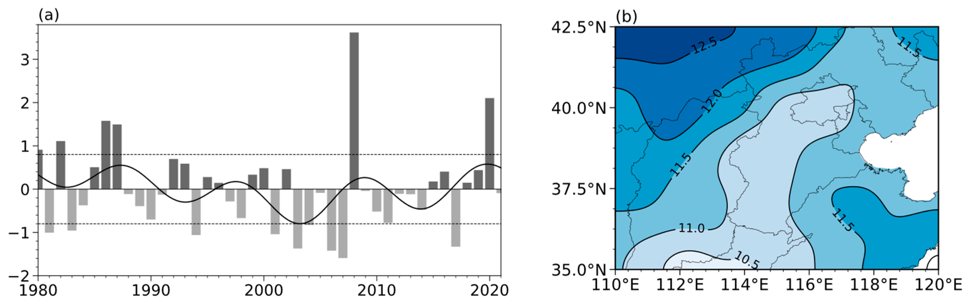
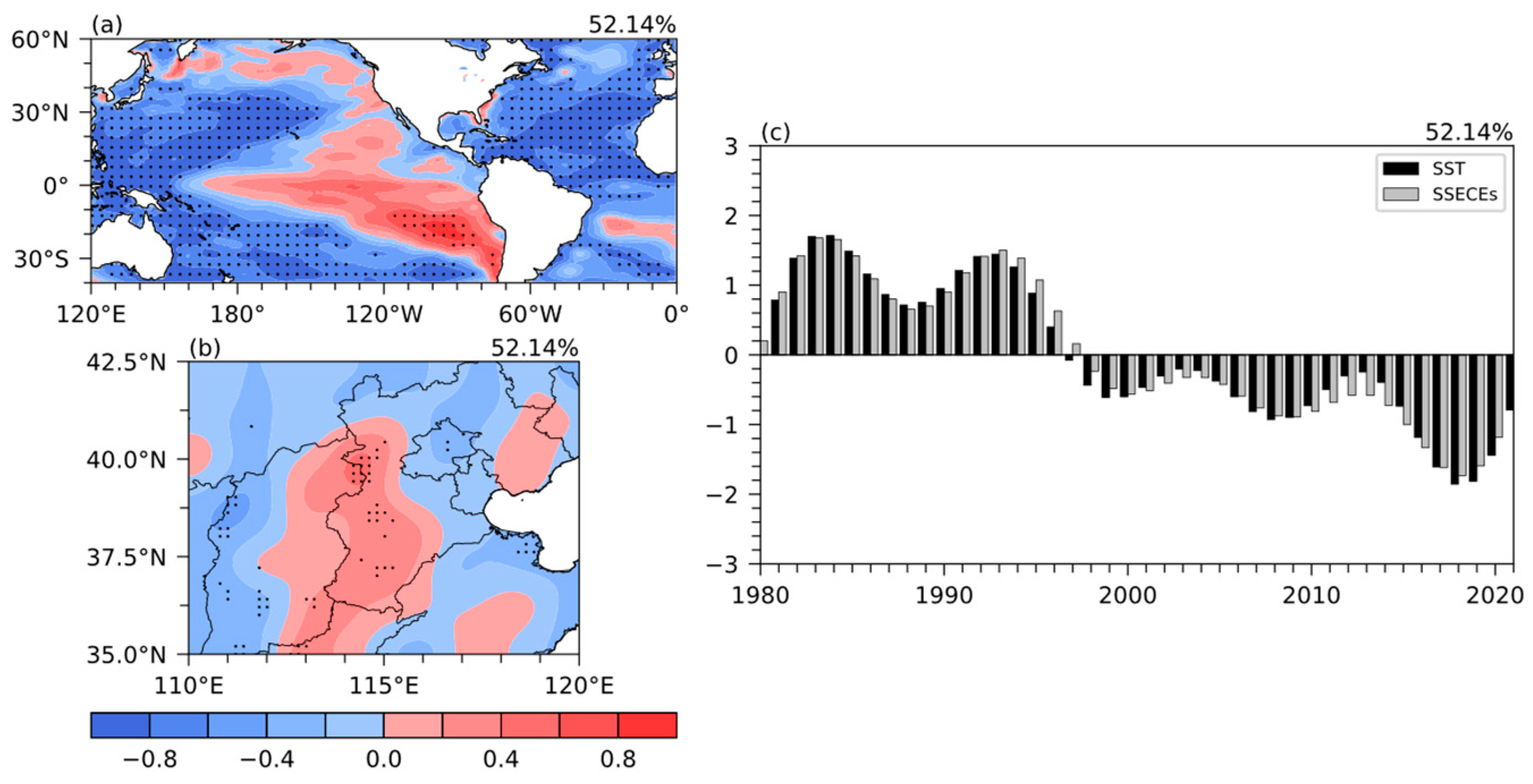
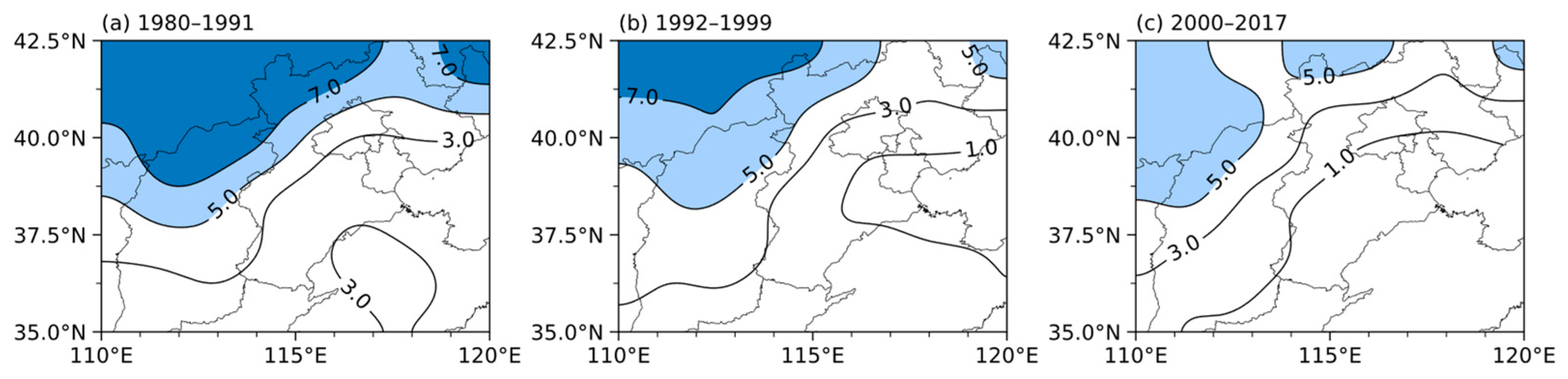
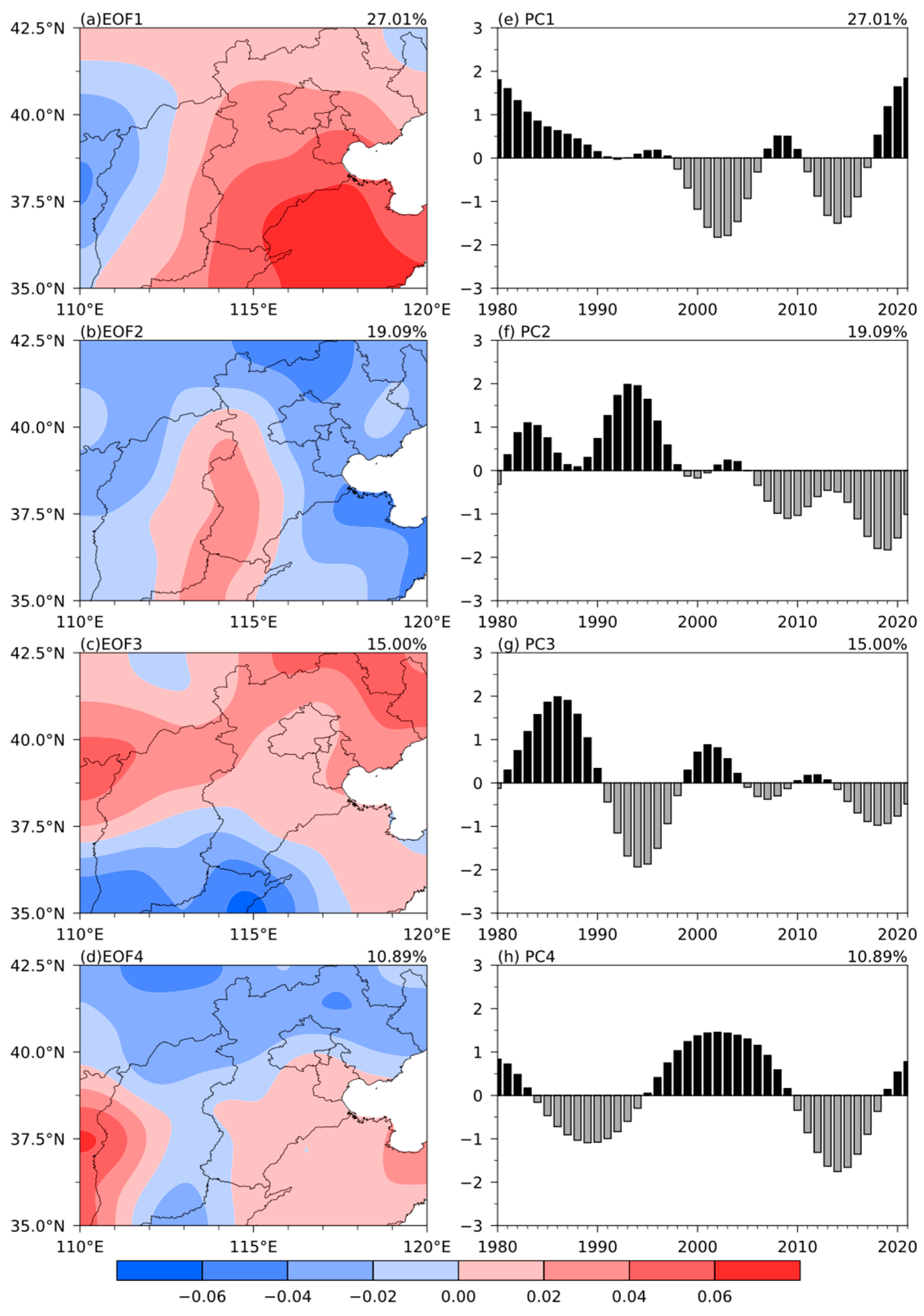
The SSECE frequency in North China showed an interdecadal transition around 1991, with frequent occurrence before 1991, less from 1992 to 2017, and increasing again since 2018. The frequency of SSECEs decreases from northwest to southeast. The interdecadal distributions of the SSECE frequency mainly include east–west inverse dipole mode, “n” mode, north-south inverse dipole mode, and “saddle-like” mode. The interdecadal transition point of the first mode, namely the east–west inverse dipole mode, is consistent with that of the regional average SSECE frequency in North China, and the transition point of the second mode is around 1997/1998.

(b)

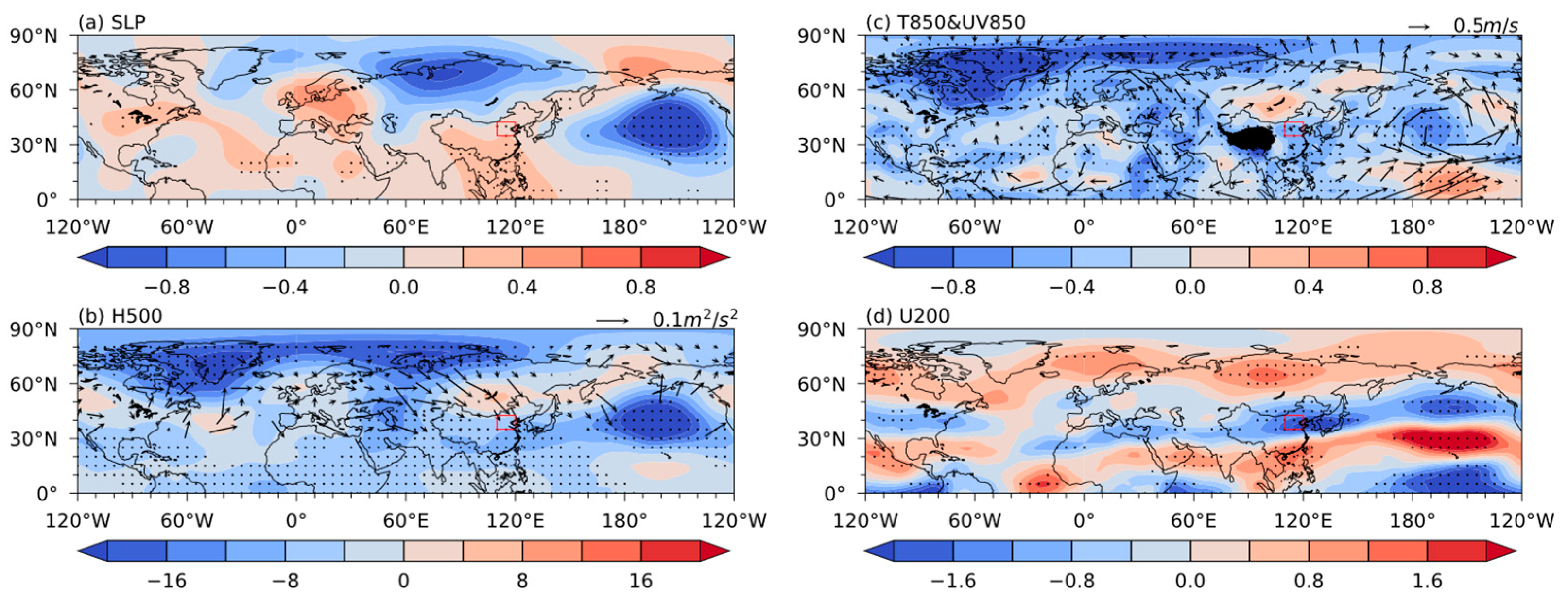
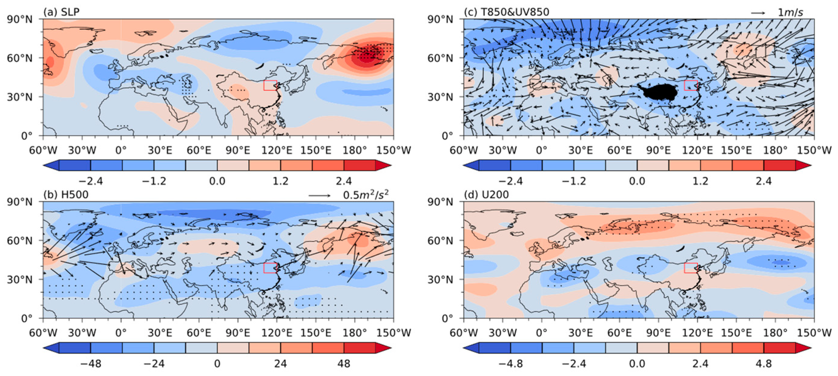
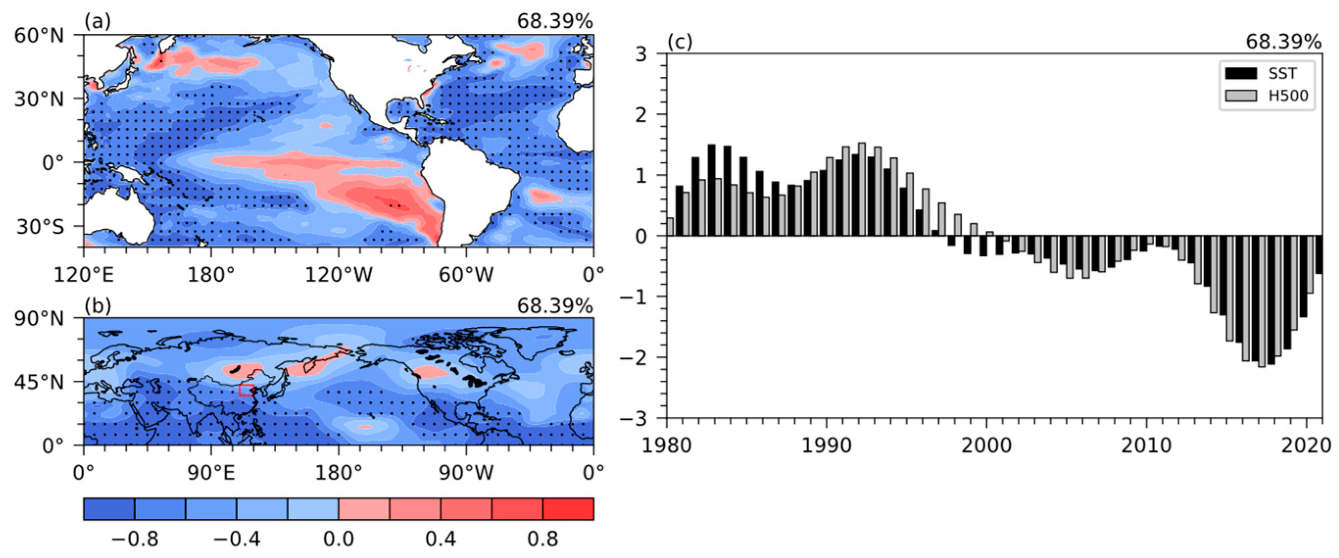
The synergistic effects of the IPO and AMO SST interdecadal anomalies may be the main reason for the “n” mode interdecadal anomalies of the SSECE frequency. Before 1997/1998, the synergisms of +IPO and −AMO stimulated the teleconnection wave train from the Pacific to Eurasia. The −EUP pattern circulation anomaly of “two troughs and one ridge” in Eurasia propagated Rossby wave energy from upstream to downstream, deepening the Urals trough and the East Asian trough, strengthening the Lake Baikal blocking High, weakening the SH in the north and strengthening in the south, combined with the strong temperate jet and weak subtropical jet in the upper troposphere. As a result, the polar cold air invades North China via the Barents Sea, West Siberia, Central Siberia, and along the northward flow in front of the Lake Baikal ridge, resulting in frequent SSECEs in central North China in winter. The opposite is true after 1997/1998.

(c)

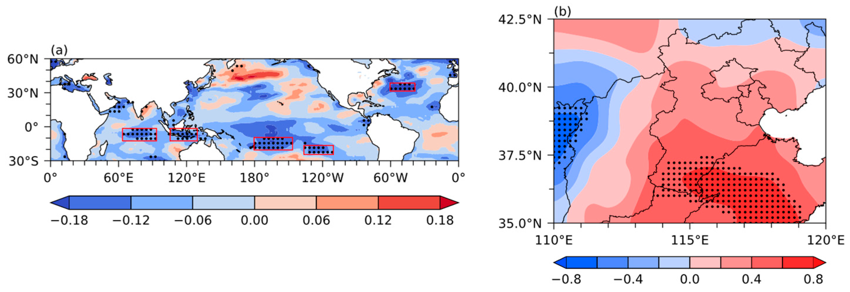
The synergistic effects of SSTAs among the Indian Ocean, Pacific, and North Atlantic may be an important reason for the east–west reverse dipole interdecadal anomaly of the SSECE frequency in North China in winter. Before 1991, the SST in the central North Atlantic was higher, and lower in the equatorial Indian Ocean and the tropical southwest Pacific, which caused a “+”, “−”, “+”, and “−” anomalous wave trains at mid-latitudes from the Atlantic to the North Pacific in the middle and lower troposphere. The Rossby wave energy propagated eastward from the North Atlantic, resulting in the stronger SH, and deeper Aleutian Low with a southerly location, stronger Urals blocking high, and deeper East Asian trough being located westward. The northerly airflow in front of the Urals ridge and behind the East Asian trough guided the polar cold air to travel southward along Novaya Zemlya, Western Siberian Plain, Inner Mongolia, and to reach North China, leading to the frequent occurrence of SSECEs in winter in central-eastern China before 1991, the opposite is true between 1992 and 2018.

4.2. Discussion

Previous studies [26] have mainly explored the influences of the interannual mid-latitude SSTAs on the winter SSECE frequency in North China. The interaction between the “El-Niño-like” SSTAs in the North Pacific and the “reversed C” negative anomalies in the North Atlantic in winter lead to a significant increase in the SSECE frequency in North China. This paper further analyzes the interdecadal characteristics of the SSECE frequency, focusing on the possible causes of the east–west inverse and “n” patterns. The interaction between IPO and AMO may be the main reason for the “n” pattern of the SSECE frequency. The cooperation of the SSTAs in the North Atlantic, the equatorial Indian Ocean, and the tropical southwest Pacific lead to the east–west inverse anomaly of the SSECE frequency in North China.

Liess et al. [31] show that a circumglobal wave train originates in the subtropical Atlantic and propagates northeastward toward the north of the West Siberian Plain, where it becomes deflected southeastward through central Asia and southern East Asia. Two positive anomalies in geopotential height over eastern Europe and Lake Baikal indicate the incoming and outgoing ends of the deflected Rossby wave train. This wave train resembles that which is detected in the present study (Figure 8), which causes the “n” pattern interdecadal anomaly of the SSECE frequency. This wave train reveals the existence of the subtropical bridge between the tropical eastern Pacific and subtropical North Atlantic [82,83]. In general, the AMO influence on Rossby wave activity in the subtropical North Atlantic suggests a multidecadal component in the detected wave train [31]; they find a link between AMO and the background state of ENSO. The IPO is the interdecadal variation of ENSO [84], this present study further suggests the interaction of IPO and AMO in triggering a similar wave train related to affect an “n” pattern on an interdecadal scale (Figure 6 and Figure 7).

Hu and Feng [85] suggest that the AMO causes an asymmetry in precipitation response to El Niño and La Niña. Thereby, further research is needed to determine whether AMO causes the asymmetry in the winter climate response to different IPO phases in North China. In addition, this paper only analyzes the first and second modes; so, what causes the third and fourth modes? The impact mechanism of the SST on the interdecadal SSECE frequency in winter in North China is still needed to further explore by numerical simulation in the future.

References

1. Seneviratne, S.I.; Nicholls, N.; Easterling, D.; Goodess, C.M.; Kanae, S.; Kossin, J.; Luo, Y.; Marengo, J.; McInnes, K.; Rahimi, M.; et al. 2012: Changes in climate extremes and their impacts on the natural physical environment. In Managing the Risks of Extreme Events and Disasters to Advance Climate Change Adaptation; Field, C.B., Barros, V., Stocker, T.F., Qin, D., Dokken, D.J., Ebi, K.L., Mastrandrea, M.D., Mach, K.J., Plattner, G.-K., Allen, S.K., et al., Eds.; A Special Report of Working Groups I and II of the Intergovernmental Panel on Climate Change (IPCC); Cambridge University Press: Cambridge, UK; New York, NY, USA, 2012; pp. 109–230. [Google Scholar] [CrossRef]
2. Donat, M.G.; Alexander, L.V.; Yang, H.; Durre, I.; Vose, R.; Dunn, R.J.H.; Willett, K.M.; Aguilar, E.; Brunet, M.; Caesar, J.; et al. Updated Analyses of Temperature and Precipitation Extreme Indices since the Beginning of the Twentieth Century: The HadEX2 Dataset. J. Geophys. Res. Atmos. 2013, 118, 2098–2118. [Google Scholar] [CrossRef]
3. Zhou, B.T.; Qian, J. Changes of weather and climate extremes in the IPCC AR6. Clim. Chang. Res. 2021, 17, 713–718. Available online: http://www.climatechange.cn/CN/10.12006/j.issn.1673-1719.2021.167 (accessed on 15 May 2023).
4. Wei, J.H.; Lin, Z.H. The Leading Mode of Wintertime Cold Wave Frequency in Northern China during the Last 42 Years and Its Association with Arctic Oscillation. Atmos. Ocean. Sci. Lett. 2009, 2, 130–134. [Google Scholar] [CrossRef]
5. Yao, Y.M.; Yao, L.; Deng, W.T. Analysis of the frequency characteristics of the similar cold wave in the middle and lower reaches of the Yangtze River. Meteorol. Mon. 2011, 37, 339–344. Available online: https://d.wanfangdata.com.cn/periodical/qx201103012 (accessed on 15 May 2023).
6. Wu, H.Y.; Du, Y.D. Climatic characteristics of cold caves in South China in the period 1961-2008. Clim. Chang. Res. 2010, 6, 192–197. [Google Scholar] [CrossRef]
7. Kang, Z.M.; Jin, R.H.; Bao, Y.Y. Characteristic analysis of cold wave in China during the period of 1951–2006. Plateau Meteorol. 2010, 29, 420–428. Available online: http://www.gyqx.ac.cn/CN/Y2010/V29/I2/420 (accessed on 15 May 2023).
8. Ding, Y.H.; Wang, Z.Y.; Song, Y.F.; Zhang, J. Causes of the unprecedented freezing disaster in January 2008 and its possible association with global warming. Acta Meteorol. Sin. 2008, 66, 808–825. [Google Scholar] [CrossRef]
9. Gao, H.; Chen, L.J.; Jia, X.L.; Ke, Z.J.; Han, Z.Q.; Zhang, P.Q.; Wang, Q.Y.; Sun, C.H.; Zhu, Y.F.; Li, W.; et al. Analysis of the severe cold surge, ice-snow and frozen disasters in South China during January 2008 II. possible climatic causes. Meteorol. Mon. 2008, 34, 101–106. Available online: https://d.wanfangdata.com.cn/periodical/qx200804013 (accessed on 15 May 2023).
10. Miao, C.S.; Zhao, Y.; Wang, J.H. Numerical simulation of 080125 cold air, freezing rain, and snow in Southern China. Trans. Atmos. Sci. 2010, 33, 25–33. [Google Scholar] [CrossRef]
11. Lu, C.H.; Wang, R.; Qin, Y.J.; Ma, L.B. Effect of stratospheric downward propagation on the large-scale snowfall of Northern Hemisphere in December 2009. Trans. Atmos. Sci. 2012, 35, 304–310. [Google Scholar] [CrossRef]
12. Shi, C.H.; Cai, W.Y.; Jin, X. Modulation by transient waves of atmospheric longwave anomalies: Dynamic mechanism of the super cold wave in South China in the extremely strong El Niño of 2015/2016. Trans. Atmos. Sci. 2016, 39, 827–834. [Google Scholar] [CrossRef]
13. Li, F.; Jiao, M.Y.; Ding, Y.H.; Jin, R.H. Climate Change of Arctic Atmospheric Circulation in Last 30 Years and Its Effect on Strong Cold Events in China. Plateau Meteorol. 2006, 25, 209–219. [Google Scholar] [CrossRef]
14. Wang, Z.Y.; Ding, Y.H. Climate change of the cold wave frequency of China in the last 53 years and the possible reasons. Chin. J. Atmos. Sci. 2006, 30, 1068–1076. [Google Scholar] [CrossRef]
15. Fu, D.X.; Sun, Z.B.; Li, Z.X.; Ni, D.H. Spatial and temporal features of China’s extreme minimum temperature in winter half year during 1955–2006. J. Meteorol. Sci. 2011, 31, 274–281. [Google Scholar] [CrossRef]
16. Ma, T.T.; Wu, Z.W.; Jiang, Z.H. How does cold wave frequency in China respond to a warming climate. Clim. Dyn. 2012, 39, 2487–2496. [Google Scholar] [CrossRef]
17. Wang, H.J. Preliminary results of the 973 project on the energy and water cycle and their role in extreme climate of China. Adv. Earth Sci. 2010, 25, 563–570. Available online: http://www.adearth.ac.cn/CN/10.11867/j.issn.1001-8166.2010.06.0563 (accessed on 15 May 2023).
18. Ren, G.Y.; Feng, G.L.; Yan, Z.W. Progresses in observation studies of climate extremes and changes in mainland China. Clim. Environ. Res. 2010, 15, 337–353. [Google Scholar] [CrossRef]
19. Wang, D.; You, Q.L.; Jiang, Z.H.; Wu, W.B.; Jiao, Y. Analysis of Extreme Temperature Changes in China based on the Homogeneity-Adjusted Data. Plateau Meteorol. 2016, 35, 1352–1363. Available online: http://www.gyqx.ac.cn/CN/10.7522/j.issn.1000–0534.2016.00019 (accessed on 15 May 2023).
20. Xie, S.Q.; Lu, C.H. Intensification of winter cold events over the past 16 years in the mid-latitudes of Eurasia and their causes. Trans. Atmos. Sci. 2018, 41, 423–432. [Google Scholar] [CrossRef]
21. Yang, J.H.; Shen, Y.P.; Wang, P.X.; Yang, Q.G. Extreme low temperature events in northwest China and their response to regional warming in the recent 45 Years. J. Glaciol. Geocryol. 2007, 29, 536–542. [Google Scholar] [CrossRef]
22. Chen, S.Y.; Wang, J.S.; Ren, Y.; Qiao, L. Evaluative Characteristic of Extreme Minimum Temperature of Northwest China in Recent 49 Years. Plateau Meteorol. 2011, 30, 1266–1273. Available online: http://www.gyqx.ac.cn/CN/Y2011/V30/I5/1266 (accessed on 15 May 2023).
23. Zhang, F.Y.; Xu, H.M. Spatial/temporal variations of spring extreme low temperature in Northeast China and its relationship with SSTA in Atlantic Ocean. Trans. Atmos. Sci. 2011, 34, 574–582. [Google Scholar] [CrossRef]
24. Qin, Y.L. Variation of Extreme Temperature in Northeast China and Its Relations with Atmospheric Circulation During Summertime. Master’s Thesis, Nanjing University of Information Science & Technology, Nanjing, China, 2012. [Google Scholar]
25. Liu, Y.; Guo, P.W.; Feng, T. The relationship between winter persistent abnormal low temperature in North China and atmospheric low frequency oscillation activities. Trans. Atmos. Sci. 2016, 39, 370–380. [Google Scholar] [CrossRef]
26. Li, L.P.; Ni, W.J.; Li, Y.G.; Guo, D.; Gao, H. Impacts of Sea Surface Temperature and Atmospheric Teleconnection Patterns in the Northern Mid-Latitudes on Winter Extremely Cold Events in North China. Adv. Meteorol. 2021, 2021, 8853457. [Google Scholar] [CrossRef]
27. Li, C.Y.; He, J.H.; Zhu, J.H. A review of decadal/interdecadal climate variation studies in China. Adv. Atmos. Sci. 2004, 21, 425–436. [Google Scholar] [CrossRef]
28. Zhang, Q.Y.; Tao, S.Y.; Peng, J.B. The studies of meteorological disasters over China. Chin. J. Atmos. Sci. 2008, 32, 815–825. [Google Scholar] [CrossRef]
29. Wei, K.; Chen, W.; Zhou, W. Changes in the East Asian cold season since 2000. Adv. Atmos. Sci. 2011, 28, 69–79. [Google Scholar] [CrossRef]
30. Wallace, J.M.; Gutzler, D.S. Teleconnections in the Geopotential Height Field during the Northern Hemisphere Winter. Mon. Weather Rev. 1981, 109, 784–812. [Google Scholar] [CrossRef]
31. Liess, S.; Agrawal, S.; Chatterjee, S.; Kumar, V. A teleconnection between the West Siberian Plain and the ENSO region. J. Clim. 2017, 30, 301–315. [Google Scholar] [CrossRef]
32. Bueh, C.; Fu, X.Y.; Xie, Z.W. Large-Scale Circulation Features Typical of Wintertime Extensive and Persistent Low Temperature Events in China. Atmos. Ocean. Sci. Lett. 2011, 4, 235–241. [Google Scholar] [CrossRef]
33. Tan, B.K.; Chen, W. Progress in the study of the dynamics of extratropical atmospheric teleconnection patterns and their impacts on East Asian climate. Acta Meteorol. Rev. 2014, 75, 908–925. [Google Scholar] [CrossRef]
34. Liu, Y.Z.; Wang, L. Interdecadal changes of scandinavian teleconnection pattern in the late 1970s. Clim. Environ. Res. 2014, 19, 371–382. [Google Scholar] [CrossRef]
35. Zhou, P.; Suo, L.; Yuan, J.; Tan, B. The East Pacific Wavetrain: Its Variability and Impact on the Atmospheric Circulation in the Boreal Winter. Adv. Atmos. Sci. 2012, 29, 471–483. [Google Scholar] [CrossRef]
36. Wang, L.; Liu, Y.Y.; Zhang, Y.; Chen, W.; Chen, S.F. Time-varying structure of the wintertime Eurasian pattern: Role of the North Atlantic sea surface temperature and atmospheric mean flow. Clim. Dyn. 2019, 52, 2467–2479. [Google Scholar] [CrossRef]
37. Ding, Y.H. Physical problems in the global climate change. Physics 2009, 38, 71–83. [Google Scholar] [CrossRef]
38. Li, C.Y. On possible mechanisms of interdecadal climate variability. Clim. Environ. Res. 2019, 24, 1–21. [Google Scholar] [CrossRef]
39. Zhu, Y.F.; Tan, G.R.; Wang, Y.G. Variation of spatial mode for winter temperature in China and its relationship with the large scale atmospheric circulation. Clim. Chang. Res. 2007, 3, 266–270. [Google Scholar] [CrossRef]
40. Ding, Y.H. Build-up, air mass transformation and propagation of Siberian high and its relations to cold surge in East Asia. Meteorl. Atmos. Phys. 1990, 44, 281–292. [Google Scholar] [CrossRef]
41. Zhang, Y.; Sperber, K.R.; Boyle, J.S. Climatology and interannual variation of the east Asian winter monsoon: Results from the 1979-95 NCEP/NCAR reanalysis. Mon. Weather Rev. 1997, 125, 2605–2619. [Google Scholar] [CrossRef]
42. Gong, D.Y.; Ho, C.H. The Siberian High and climate change over middle to high latitude Asia. Theor. Appl. Climatol. 2002, 72, 1–9. [Google Scholar] [CrossRef]
43. Thompson, D.W.; Wallace, J.M. The Arctic oscillation signature in the wintertime geopotential height and temperature fields. Geophys. Res. Lett. 1998, 25, 1297–1300. [Google Scholar] [CrossRef]
44. Van, L.H.; Rogers, J.C. The Seesaw in Winter Temperatures between Greenland and Northern Europe. Part I: General Description. Mon. Weather Rev. 1978, 106, 296–310. [Google Scholar] [CrossRef]
45. Wu, B.Y.; Huang, R.H. Effects of the Extremes in the North Atlantic Oscillation on East Asia Winter Monsoon. Chin. J. Atmos. Sci. 1999, 23, 641–651. [Google Scholar] [CrossRef]
46. Han, F.H.; Chen, H.S.; Ma, H.D. Interdecadal Variations in the Relationship between the Winter North Atlantic Oscillation and Extreme Low Temperature over Northern China. Chin. J. Atmos. Sci. 2018, 42, 239–250. [Google Scholar] [CrossRef]
47. Zuo, J.Q.; Ren, H.L.; Li, W.J.; Wang, L. Interdecadal Variations in the Relationship between the Winter North Atlantic Oscillation and Temperature in South-Central China. J. Clim. 2016, 29, 7477–7493. [Google Scholar] [CrossRef]
48. Li, C.Y.; Liao, Q.H. Quasi-decadal oscillation of climate in East Asia/northwestern Pacific region and possible mechanism. Clim. Environ. Res. 1996, 1, 124–133. [Google Scholar] [CrossRef]
49. Gu, W.; Li, C.Y.; Wang, X.; Zhou, W.; Li, W.J. Linkage between Mei-yu precipitation and North Atlantic SST on the decadal timescale. Adv. Atmos. Sci. 2009, 26, 101–108. [Google Scholar] [CrossRef]
50. Minobe, S.; Mantua, N. Interdecadal modulation of interannual atmospheric and oceanic variability over the North Pacific. Prog. Oceanogr. 1999, 43, 163–192. [Google Scholar] [CrossRef]
51. Liu, Q.Y.; Li, C.; Hu, R.J. Interdecadal oscillations in the North Pacific and global warming. Clim. Environ. Res. 2010, 15, 217–224. [Google Scholar] [CrossRef]
52. Mantua, N.J.; Hare, S.R.; Zhang, Y.; Wallace, J.M.; Francis, R.C. A Pacific interdecadal climate oscillation with impacts on salmon production. Bull. Amer. Meteor. Soc. 1997, 78, 1069–1079. [Google Scholar] [CrossRef]
53. Li, C.Y.; Xian, P. Interdecadal variation of SST in the North Pacific and the anomalies of atmospheric circulation and climate. Clim. Environ. Res. 2003, 8, 258–273. [Google Scholar] [CrossRef]
54. Yang, X.Q.; Zhu, Y.M.; Xie, Q.; Ren, X.J.; Xu, G.Y. Advances in studies of Pacific Decadal Oscillation. Chin. J. Atmos. Sci. 2004, 28, 979–992. [Google Scholar] [CrossRef]
55. Li, L.P.; Wang, P.X.; Zheng, X.Y. Diagnostic analysis on temporal-spatial characteristics of sub-surface sea temperature and air-sea interaction over the North Pacific. J. Nanjing Inst. Meteorol. 2003, 26, 145–154. [Google Scholar] [CrossRef]
56. Gallego, B.; Cessi, P. Decadal variability of two oceans and an atmosphere. J. Clim. 2001, 14, 2815–2832. [Google Scholar] [CrossRef]
57. Zhu, Y.M.; Yang, X.Q.; Xie, Q.; Yu, Y.Q. The Covariant modes between sea surface temperature in the Pacific Ocean and mid-latitude in the northern hemisphere atmospheric circulation anomalies in winter. Prog. Nat. Sci. 2008, 18, 161–171. [Google Scholar] [CrossRef]
58. McCabe, G.J.; Palecki, M.A.; Betancourt, J.L. Pacific and Atlantic Ocean influences on multidecadal drought frequency in the United States. Proc. Natl. Acad. Sci. USA 2004, 101, 4136–4141. [Google Scholar] [CrossRef]
59. Chen, J.Y.; Delgenio, A.D.; Carlson, B.E.; Bosilovich, M.G. The spatiotemporal structure of twentieth-century climate variations in observations and reanalyses. Part II: Pacific pan-decadal Variability. J. Clim. 2008, 21, 2634–2650. [Google Scholar] [CrossRef]
60. Dong, B.; Dai, A.G. The influence of the Interdecadal Pacific Oscillation on Temperature and Precipitation over the Globe. Clim. Dyn. 2015, 45, 2667–2681. [Google Scholar] [CrossRef]
61. Li, S.L. Impact of Northwest Atlantic SST anomalies on the circulation over the Ural Mountains during early winter. J. Meteorol. Soc. Jpn. 2004, 82, 971–988. [Google Scholar] [CrossRef]
62. Qu, J.H.; Jiang, Z.H.; Tan, G.R.; Sun, L. Relation between interannual, interdecadal variability of SST in North Atlantic in winter and air temperature in China. Sci. Geogr. Sin. 2006, 26, 557–563. [Google Scholar] [CrossRef]
63. Li, S.L.; Bates, G.T. Influence of the Atlantic multidecadal oscillation on the winter climate of East China. Adv. Atmos. Sci. 2007, 24, 126–135. [Google Scholar] [CrossRef]
64. Ding, T.; Qian, W.H.; Yan, Z.W. Characteristics and changes of cold surge events over China during 1960–2007. Atmos. Ocean. Sci. Lett. 2009, 2, 339–344. [Google Scholar] [CrossRef]
65. Liu, J.; Xu, X.F.; Luo, H. Econometric Analysis of the Impact of Climate Extremes on Agricultural Economic Output in China. Sci. China Earth Sci. 2012, 42, 1076–1082. [Google Scholar] [CrossRef]
66. Kalnay, E.; Kanamitsu, M.; Kistler, R.; Collins, W.; Deaven, D.; Gandin, L.; Joseph, D.; Iredell, M.; Saha, S.; White, G.; et al. The NCEP/NCAR 40-year reanalysis project. Bull. Amer. Meteor. Soc. 1996, 77, 437–472. Available online: https://www.jstor.org/stable/26232740 (accessed on 15 May 2023). [CrossRef]
67. Ishii, M.; Shouji, A.; Sugimoto, S.; Matsumoto, T. Objective Analyses of Sea-Surface Temperature and Marine Meteorological Variables for the 20th Century Using ICOADS and the Kobe Collection. Int. J. Climatol. 2005, 25, 865–879. [Google Scholar] [CrossRef]
68. GB/T 20484–2017; Grade of Cold Air. Standards Press of China: Beijing, China, 2017.
69. GB/T 21987–2017; Grades of Cold Wave. Standards Press of China: Beijing, China, 2017.
70. Li, L.P.; Wang, P.X.; Li, H. Interdecadal and interannual variabilities of air and sea and their relations over the Pacific. Acta Meteorol. Sin. 2004, 18, 227–244. Available online: http://jmr.cmsjournal.net/en/article/id/956 (accessed on 15 May 2023).
71. Ji, C.X.; Zhang, Y.Z.; Cheng, Q.M.; Li, Y.; Jiang, T.C.; Liang, X.S. On the relationship between the early spring Indian Ocean’s sea surface temperature (SST) and the Tibetan Plateau atmospheric heat source in summer. Glob. Planet. Chang. 2018, 164, 1–10. [Google Scholar] [CrossRef]
72. Ashok, K.; Guan, Z.Y.; Yamagata, T. Influence of the Indian Ocean Dipole on the Australian winter rainfall. Geophys. Res. Lett. 2003, 30, 1821. [Google Scholar] [CrossRef]
73. Wu, F.M.; Li, W.K.; Zhang, P.; Li, W. Relative Contributions of Internal Atmospheric Variability and Surface Processes to the Interannual Variations in Wintertime Arctic Surface Air Temperatures. J. Clim. 2021, 34, 7131–7148. [Google Scholar] [CrossRef]
74. Takaya, K.; Nakamura, H. A Formulation of a Phase-Independent Wave-Activity Flux for Stationary and Migratory Quasigeostrophic Eddies on a Zonally Varying Basic Flow. J. Atmos. Sci. 2001, 58, 608–627. [Google Scholar] [CrossRef]
75. Wu, H.B.; Wu, L. Diagnosis and Prediction Method of Climate Variability; China Meteorological Press: Beijing, China, 2005; pp. 208–225. [Google Scholar]
76. Wei, F.Y. Modern Climate Statistical Diagnosis and Prediction Techniques, 2nd ed.; China Meteorological Press: Beijing, China, 2007; pp. 10–28. [Google Scholar]
77. Wang, P.X.; Duan, M.K.; Li, L.P.; Lu, C.H.; Guo, D.; Sun, X.J. Basic Analysis Method of Atmospheric Circulation and its Application; Science Press: Beijing, China, 2019; pp. 153–165. [Google Scholar]
78. North, G.R.; Bell, T.L.; Cahalan, R.F. Sampling Errors in the Estimation of Empirical Orthogonal Functions. Mon. Weather Rev. 1982, 110, 699–706. [Google Scholar] [CrossRef]
79. Tian, X.X.; Shou, S.W. Analysis of isentropic vorticity for two cold wave processes in Dec. 2008. J. Meteorol. Sci. 2013, 33, 102–108. [Google Scholar] [CrossRef]
80. Tang, W.Y.; Sun, Z.B. Effect of Indian Ocean SSTA on China Temperature Anomaly. J. Nanjing Inst. Meteorol. 2007, 30, 667–673. [Google Scholar] [CrossRef]
81. Zheng, F.; Yuan, Y.; Ding, Y.H.; Li, K.X.; Fang, X.H.; Zhao, Y.H.; Sun, Y.; Zhu, J.; Ke, Z.J.; Wang, J.; et al. The 2020/21 Extremely Cold Winter in China Influenced by the Synergistic Effect of La Niña and Warm Arctic. Adv. Atmos. Sci. 2022, 39, 546–552. [Google Scholar] [CrossRef]
82. Graf, H.F.; Zanchettin, D. Central Pacific El Niño, the “subtropical bridge”, and Eurasian climate. J. Geophys. Res. 2012, 117, D01102. [Google Scholar] [CrossRef]
83. Park, J.; Dusek, G. ENSO components of the Atlantic multidecadal oscillation and their relation to North Atlantic interannual coastal sea level anomalies. Ocean Sci. 2013, 9, 535–543. [Google Scholar] [CrossRef]
84. Dong, B.; Dai, A.G.; Vuille, M.; Timm, O.E. Asymmetric Modulation of ENSO Teleconnections by the Interdecadal Pacific Oscillation. J. Clim. 2018, 31, 7337–7361. [Google Scholar] [CrossRef]
85. Hu, Q.; Feng, S. AMO-and ENSO-Driven Summertime Circulation and Precipitation Variations in North America. J. Clim. 2012, 25, 6477–6495. [Google Scholar] [CrossRef]
Figure 1. Distribution of 396 stations in North China.
Atmosphere 14 01699 g001
Figure 2. (a) Standardized time series of the winter regional average SSECE frequency (histogram) and its interdecadal components (curve) in North China from 1980 to 2021, dashed line represents 0.8. (b) Spatial distribution of averaged cooling amplitude of all SSECEs during 1980–2021 (unit: °C).
Atmosphere 14 01699 g002
Figure 3. Spatial distribution of the winter SSECE frequency averaged in North China during the frequent (a), transitional (b), and infrequent (c) periods. Unit: number of occurrences.
Atmosphere 14 01699 g003
Figure 4. The first four EOF eigenvectors (ad) and their standardized time coefficient series (eh) of the interdecadal components of the SSECE frequency in winter in North China.
Atmosphere 14 01699 g004
Figure 5. The first SVD heterogeneous correlations between the interdecadal components of the SST (a) and the SSECE frequency in North China (b) in winter and their normalized temporal coefficient series from 1980–2021 (c). The dotted areas are statistically significant at the 95% confidence level.
Atmosphere 14 01699 g005
Figure 6. The figure is the same as Figure 5, but for the first SVD mode between SST (a) and H500 (b) in winter and their normalized temporal coefficient series from 1980–2021 (c).
Atmosphere 14 01699 g006
Figure 7. The figure is the same as Figure 5, but for the first SVD mode between H500 (a) and SSECE frequency (b) in winter and their normalized temporal coefficient series from 1980–2021 (c).
Atmosphere 14 01699 g007
Figure 8. Linear regression coefficients of the first SVD SST temporal coefficient between the interdecadal components of SST and SSECE frequency on the (a) SLP (unit: hPa), (b) H500 (shading, unit: gpm) and T-N wave activity flux (vector, unit: m2/s2), (c) T850 (shading, unit: °C, the blank area is the Tibetan Plateau) and UV850 (vector, unit: m/s), (d) U200 (unit: m/s) fields in winter. The red rectangle shows the location of North China. The areas with dots represent statistical significance at the 90% confidence level based on the Student’s t-test.
Atmosphere 14 01699 g008
Figure 9. (a) Linear regression field of the SSECE frequency PC1 on the interdecadal SST field in winter. (b) The correlation coefficients between ISST and the interdecadal anomaly of the SSECE frequency in North China; the dotted areas are statistically significant at the 95% confidence level.
Atmosphere 14 01699 g009
Figure 10. Linear regression coefficients of the ISST on the (a) SLP (unit: hPa), (b) H500 (shading, unit: gpm) and T-N wave activity flux (vector, unit: m2/s2), (c) T850 (shading, unit: °C, the blank area is the Tibetan Plateau) and UV850 (vector, unit: m/s), (d) U200 (unit: m/s) fields in winter. The red rectangle shows the location of North China. The areas with dots represent statistical significance at the 90% confidence level based on the Student’s t-test.
Atmosphere 14 01699 g010